Review

A Collection of SAR Methodologies for Monitoring Wetlands

1
Canada Centre for Mapping and Earth Observations, Natural Resources Canada, 560 Rochester Street, Ottawa, ON K1A 0Y7, Canada
2
Science and Technology Branch, Environment Canada, Government of Canada, 4905 Dufferin Street, Toronto, ON M3H 5T4 Canada
3
Land Surface Applications (LAX), German Remote Sensing Centre (DFD), German Aerospace Center (DLR), Obserpfaffenhofen, D-82234 Wessling, Germany
4
Ducks Unlimited Canada, 1 Mallard Bay at Hwy 220, P.O. Box 1160, Stonewall, MB R0C 2Z0, Canada
*
Author to whom correspondence should be addressed.
These authors contributed equally to this work.
Remote Sens. 2015, 7(6), 7615-7645; https://doi.org/10.3390/rs70607615
Submission received: 17 January 2015 / Revised: 12 May 2015 / Accepted: 22 May 2015 / Published: 9 June 2015
(This article belongs to the Special Issue Towards Remote Long-Term Monitoring of Wetland Landscapes)

Abstract

:
Wetlands are an important natural resource that requires monitoring. A key step in environmental monitoring is to map the locations and characteristics of the resource to better enable assessment of change over time. Synthetic Aperture Radar (SAR) systems are helpful in this way for wetland resources because their data can be used to map and monitor changes in surface water extent, saturated soils, flooded vegetation, and changes in wetland vegetation cover. We review a few techniques to demonstrate SAR capabilities for wetland monitoring, including the commonly used method of grey-level thresholding for mapping surface water and highlighting changes in extent, and approaches for polarimetric decompositions to map flooded vegetation and changes from one class of land cover to another. We use the Curvelet-based change detection and the Wishart-Chernoff Distance approaches to show how they substantially improve mapping of flooded vegetation and flagging areas of change, respectively. We recommend that the increasing availability SAR data and the proven ability of these data to map various components of wetlands mean SAR should be considered as a critical component of a wetland monitoring system.

Graphical Abstract

1. Introduction

Wetlands are a critical part of our natural environment. They provide food and shelter to many types of wildlife and invertebrates, including endangered and threatened species, filter sediments and toxins [1], help prevent flooding [2,3] protect shorelines [4], store carbon, give off oxygen and water vapor [5], and provide recreational activities such as hiking and fishing. Although the importance of wetlands is widely recognized, they are currently disappearing at a dramatic rate. Approximately 25% of the world’s wetlands are located in Canada [6], and approximately 14% of the Canadian landscape is covered by wetlands. Roughly 68% of Ontario’s wetlands have been converted to agriculture or infrastructure and, similarly, there are only about 25% of the original Prairie Pothole wetlands remaining in Southwestern Manitoba [6]. There has been a 50% loss of wetlands worldwide over the last century [7], with a 6% decrease just from 1993 to 2007 [8]. In addition, wetlands are becoming fragmented or impaired and have lost the capacity to function fully because of pollution, climate change, invasive species, agricultural tile drainage, hydroelectric development, urban expansion, and recreation [9,10,11,12].
Wetlands are particularly sensitive to climate change and severe events. Wetlands are often able to recover from naturally occurring stresses, such as storms or damage from ice, but are less resilient to human-induced stresses, like industrial discharge or dredging, which usually occur quickly and impose severe impacts from which it is difficult to recover. Even small shifts in temperature or the water supply can impact wetland organisms [13]. For example, increases in temperature may allow invasive plants to outcompete native plants [14,15,16]. Moreover, high temperatures combined with low oxygen levels often lead to overgrowth of bacteria [13]. It is expected that climate change will result in longer summers and shorter, warmer winters [17,18,19,20]. Wetlands rely on cold Canadian winters to provide water from snowmelt and spring flooding [21]. Rising temperatures may result in the drying of some wetlands [22]. Thus, wetlands are dynamic and any mapping or inventory assessment should accurately reflect these dynamics.
Currently, there is no inclusive or dynamic wetland inventory or monitoring program in Canada [23,24], or globally. The majority of existing wetland research has been localized, has covered a limited time period, and has varied in approach and scale. The Canadian Wetland Inventory (CWI)—a joint initiative between the Canadian Space Agency, Ducks Unlimited Canada, Environment Canada and the North American Wetlands Conservation Council (Canada)—was established in 2002 to facilitate the creation of a national inventory to aid in wetland conservation. The CWI is still in progress, and approximately 25% of the mapping has been completed, is near completion or is still in progress [25]. To protect and monitor existing wetlands it is essential to have an inventory of where and how many wetlands currently exist and how they are changing. Wetlands are dynamic and can change significantly within an annual growing season, as well as inter-annually and over a decadal time periods [26,27]. Wetlands can transform from dry to flooded states, and vice versa [26], or be affected by various other factors like fires [28], drainage [12,29], and grazing [30]. The naturally variable states of wetlands are what make them so productive. Wetlands can vary widely due to a variety of factors including geographical location (e.g., coastal vs. inland or polar vs. tropic), rainfall, evaporation, climate change and anthropogenic influences. A study of the agricultural impacts and recovery of wetlands between 1985 and 2005 showed that wetland margins were more affected by land use than wetland basins [31], underscoring the imperative for current, accurate wetland mapping methodology and inventory so regulated wetlands can be properly monitored, managed and protected. Because wetlands are changing over both short and long time periods, frequent and consistent monitoring is needed.
Synthetic Aperture Radar (SAR) technology can be effective for monitoring changes in surface water [32,33] and wetlands both seasonally and annually [34,35,36,37]. SAR has many characteristics that make it ideal for mapping and monitoring water and wetlands over time. SAR is able to image landscape conditions night or day, through cloud cover, and in near-real time [38,39]. These are often limitations for optical/infrared satellite sensors. SAR systems also can penetrate vegetation canopies, to varying degrees, to image understory conditions [40]. Additionally, the water-saturated nature of wetlands tends to render them highly reflective of SAR transmitted energy.
Nevertheless, several factors can affect radar backscatter including seasonal timing of acquisition, look direction, incidence angle, soil moisture, dielectric constant, and the structure/composition of the ground features. SAR systems transmit microwaves with an incidence angle and a look direction on one side of the satellite. The incidence angle, which is the angle between the radar beam and the ground surface, can affect the appearance of smooth targets on the image. Smooth surfaces can appear brighter than rough surfaces at small incidence angles (usually less than 20–25 degrees), but rough surfaces remain largely unaffected by incidence angle. Lower incidence angles tend to be more sensitive to waves on water, therefore a combination of high and low incidence angle images are sometimes needed to accurately map water [40]. Smaller incidence angles are better able to penetrate vegetation, and thus can better detect flooded vegetation [41,42,43].
Water has a high dielectric constant and is a specular reflector; very little backscatter is returned to the sensor, making water appear as a dark feature [44]. However, when waves are present in water there is often an increase in backscatter, which can cause confusion with land features such as dry vegetation [40]. The majority of other natural land features, particularly vegetation canopies, are heterogeneous and have relatively high amounts of surface roughness, resulting in the radar signal being scattered diffusely, with features appearing bright on the image [40]. Differences in topography can also distort a SAR image. Foreshortening occurs when the SAR signal returns from the bottom of a tall feature facing towards the satellite prior to returning from the top of the feature. This causes the image to be compressed in the near range (the part of the image closest to the nadir track) and to be stretched in the far range (the part of the swath furthest from the nadir track). This distortion increases with small look angles and steep slopes [45]. In extreme cases the image can be distorted from layover, which occurs when the SAR signal reaches the top of the feature before the bottom in the near-range slope. Part of the image can appear missing if there is a very steep slope and a large look angle [45]. The sensitivity of SAR to the dielectric constant and roughness of features demonstrates the importance of optimizing the timing of image acquisitions. Data for mapping wetlands are best acquired in the spring, summer and fall to avoid any ice-on imagery [46]. For example, rough surface water can produce a backscatter response similar to ice, thus making it difficult to distinguish between the two land covers [46].
Additional information beyond the radiometric response provided with optical satellites can be extracted from SAR data to help detect flooded areas [47,48] and classify wetlands [35,48], based on hydrologic features and surface structure. In a single-channel SAR system both the transmitted and received energy from the satellite are either horizontally (H) or vertically (V) polarized. In dual-channel SAR systems the signal can be both co-polarized (transmitted and received energy as HH or VV) and cross-polarized (transmitted and received as HV or VH). With the advancement of fully polarimetric satellite systems such as RADARSAT-2 the satellite can transmit and receive energy in all four planes (HH, VV, HV and VH), maintaining the phase and allowing for mapping of the different scattering mechanisms within a wetland [49], rather than just the difference between low and high backscatter values (Figure 1). The phase measures the time it takes for the radar signal sent from the satellite to interact with the target on the ground and return to the satellite [50]. This allows the user to decompose the SAR backscatter being returned from the objects being sensed into four common scattering types: (1) specular scattering (no return to the SAR), which occurs from smoother surfaces such as calm water or bare soil; (2) rough scattering, which results when there is a single bounce return to the SAR from surfaces such as small shrubs or rough water; (3) volume scattering, which is when the signal is backscattered in multiple directions from features such as vegetation canopies; and (4) double-bounce or dihedral scattering, which results when two smooth surfaces create a right angle that deflects the incoming radar signal off both surfaces such that most of the energy is returned to the sensor. This latter scattering case typically occurs when vertical emergent vegetation is surrounded by a visible, smooth water surface [32,47,48,49,50,51]. Flooded vegetation can also have a combination of double-bounce and volume backscattering [50,51]. When fully polarimetric SAR images are acquired throughout the growing season, the user can analyze the backscatter response from each stage of the hydrologic and vegetation development (leaf-on and leaf-off) to better understand responses during wetter and dryer periods.
Figure 1. A comparison of how RADARSAT-1 and RADARSAT-2 transmit and receive radar waves. RADARSAT-1 transmits and receives radar waves horizontally to the target on the ground. RADARSAT-2 can transmit and receive radar waves in both the horizontal and vertical polarization plains, allowing calculation of the phase. Reproduced by permission of/or Courtesy of MacDonald, Dettwiler and Associates Ltd.
Remotesensing 07 07615 g001
Figure 2. A comparison of RADARSAT-2 and the RADARSAT Constellation Mission (RCM) swath widths. These graphics illustrate that a wider swath width will be available for many beam modes on the RCM compared to RADARSAT-2. Reproduced by permission of/or Courtesy of MacDonald, Dettwiler and Associates Ltd.
Remotesensing 07 07615 g002
The Canadian RADARSAT-2 satellite, as well as the upcoming RADARSAT Constellation Mission (RCM), offers a wide range of beam modes well suited to monitor wetlands. The Spotlight beam mode has high spatial resolution, allowing the user to detect small water bodies. The Polarimetric beam mode enables the application of polarimetric decompositions, which allow the user to decompose the scattering matrix and, as a result, better detect flooded vegetation and classify wetlands [35,49]. RCM, which is anticipated to launch in 2018, will have a baseline mission composed of 3 satellites offering an average daily coverage for 95% of the world [52]. In addition to the beam modes offered by RADARSAT-2, RCM will have a circular-linear compact polarimetry mode, which transmits a circularly polarized wave and receives on the linear, orthogonal, horizontal, and vertical planes [53]. RCM will have a shorter revisit time (four days) compared to RADARSAT-2 (24 days), due to the constellation, and a larger swath-width in some cases (e.g., 50 × 50 m2 resolution images will have a 500 km swath width with RCM compared to 300 km for RADARSAT-2) (Figure 2). This will make it possible for more frequent monitoring over wider areas. Likewise, the compact polarimetric mode will allow polarimetric information to be acquired over a wider swath.
Many studies have demonstrated SAR’s utility in mapping wetlands [35,54,55,56,57,58,59]. However, there are many different SAR techniques to extract polarimetric parameters as well as several polarimetric decompositions [35,60]. To date, there is not a well-established SAR methodology to map and monitor wetlands. In this paper we provide an overview of some current methodologies being used to map and monitor two aspects of wetlands with RASARSAT-2 data, surface water and flooded vegetation. We also describe a tool for flagging areas of change within wetlands, the Wishart-Chernoff Distance technique. We present these methodologies through case studies from several locations, and more in-depth descriptions of all are available in the original papers. Detailed descriptions of the locations of the field studies are not included here because the methods are applicable in many locations around the world.

2. Surface Water

Mapping areas of open water is an important component of wetland monitoring. SAR has been used as a tool to map open water for many purposes in a variety of locations [61,62,63,64,65]. There are several SAR-based methods for mapping open water [44]. Visual interpretation can be performed by an experienced analyst to manually map areas of water; however, this can be very time consuming and results can vary among image interpreters [44]. Multi-temporal interferometric SAR coherence (e.g., [66] is another method, based on using the constantly-changing scattering characteristics of water surfaces (from waves, resulting in low coherence) to distinguish water from land [67]. This technique is dependent on having high temporal coherence in the surrounding land cover, which can be difficult to achieve due to snow, rain, and/or wind changing the dielectric properties [68]. A third method to map surface water is through active contour models (e.g., [61,69]), which uses local tone and texture values to delineate features. Results have been promising, but there has been confusion between open water and non-flooded vegetation [61]. A texture-based method has also been developed for water mapping, which makes use of textural variation based on statistics [44]. The limitations are that it can be challenging to select the correct window size and best texture measure, and selecting a threshold value is still necessary to classify water [44]. To date grey-level thresholding is the most commonly used approach to map surface water with SAR imagery. In this method all pixels with a backscatter coefficient lower than a specified threshold in an intensity image are mapped as water [70,71]. This technique is useful for producing results quickly and inexpensively [72], but is only suitable for calm open water with a specular backscatter response [73]. A user-selected threshold was chosen to map surface water in the case study we present because it offered a flexible, efficient, and user controlled, scene specific approach.

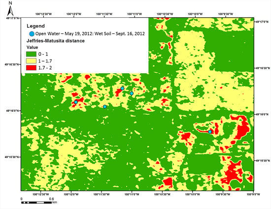
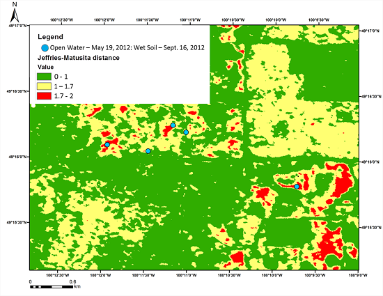
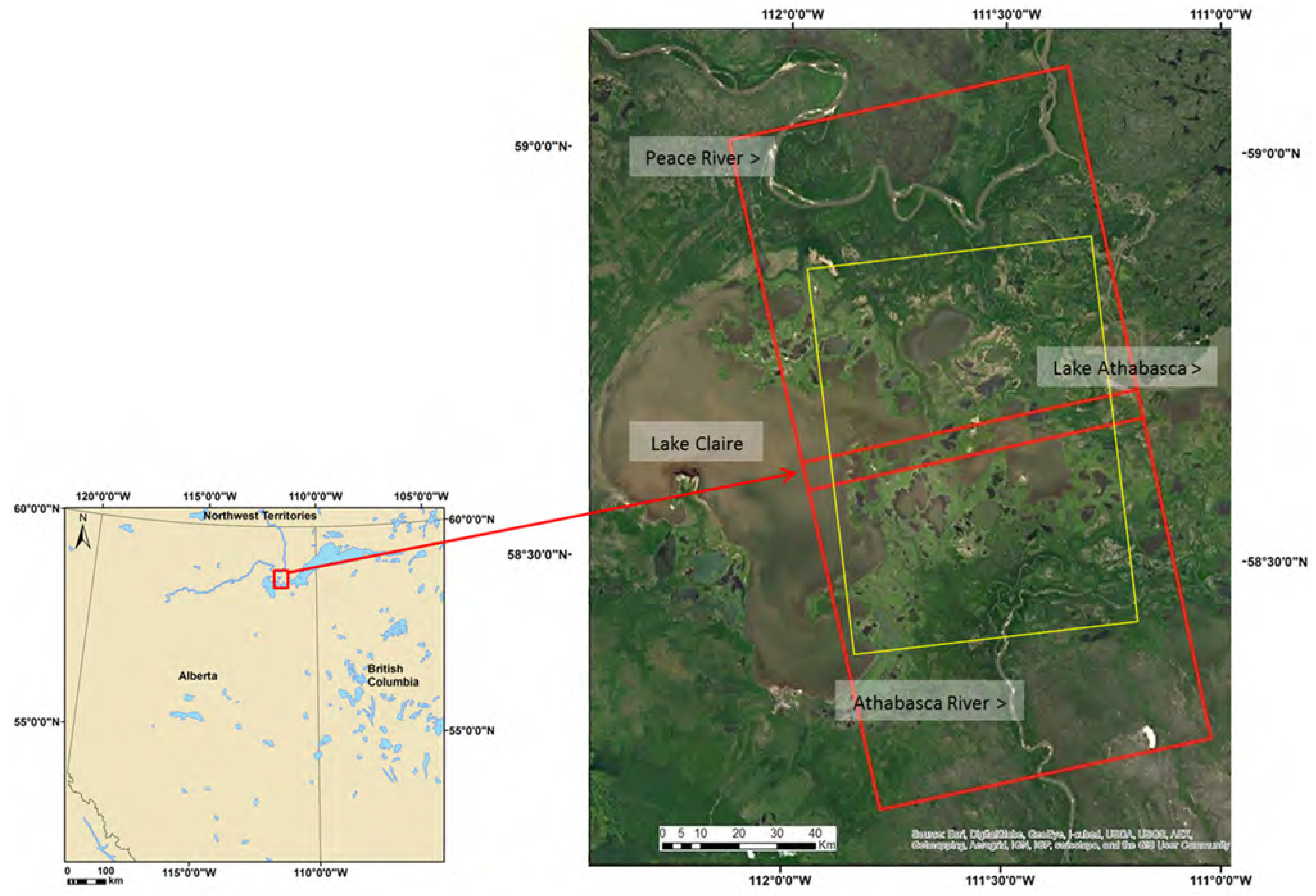
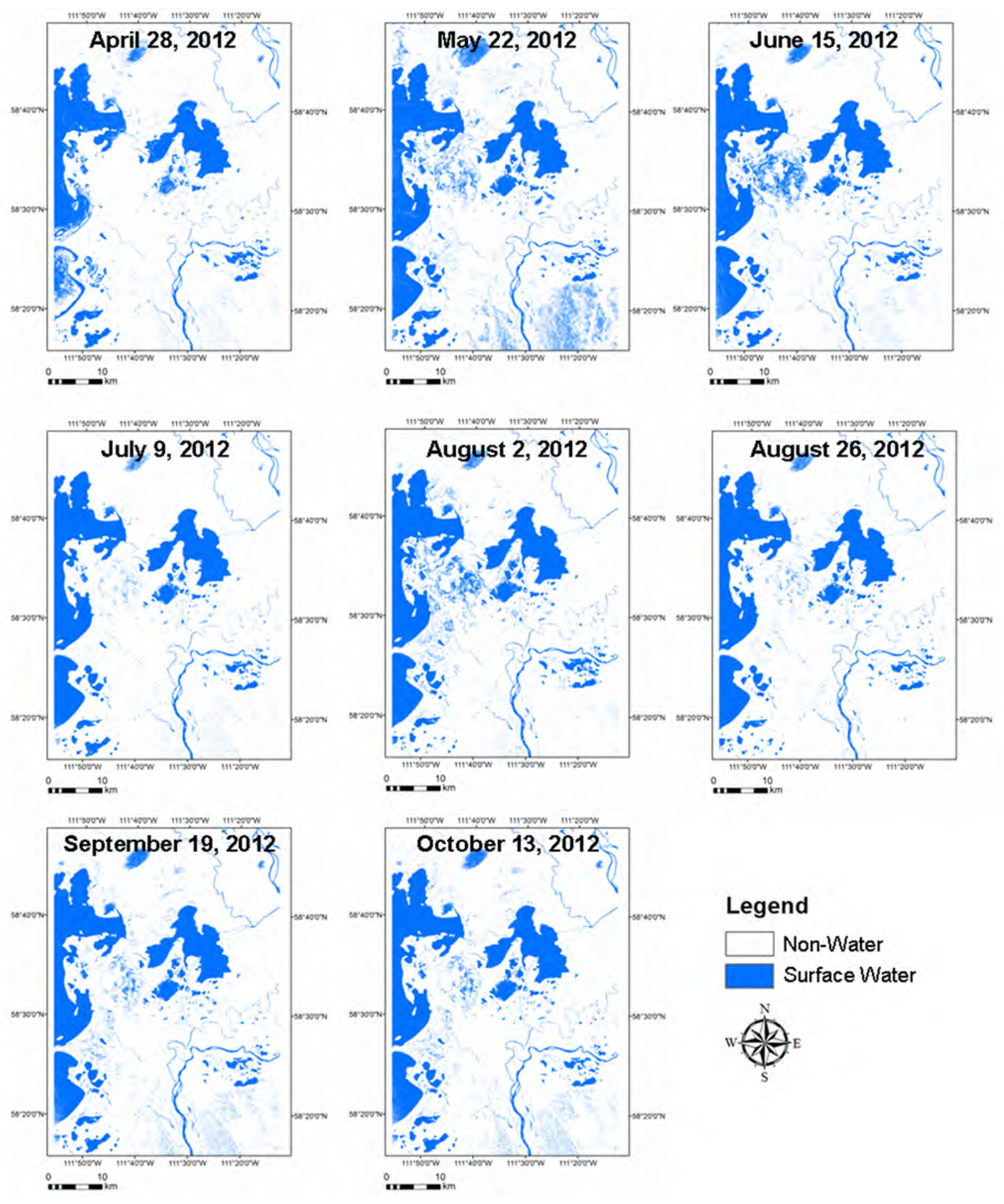
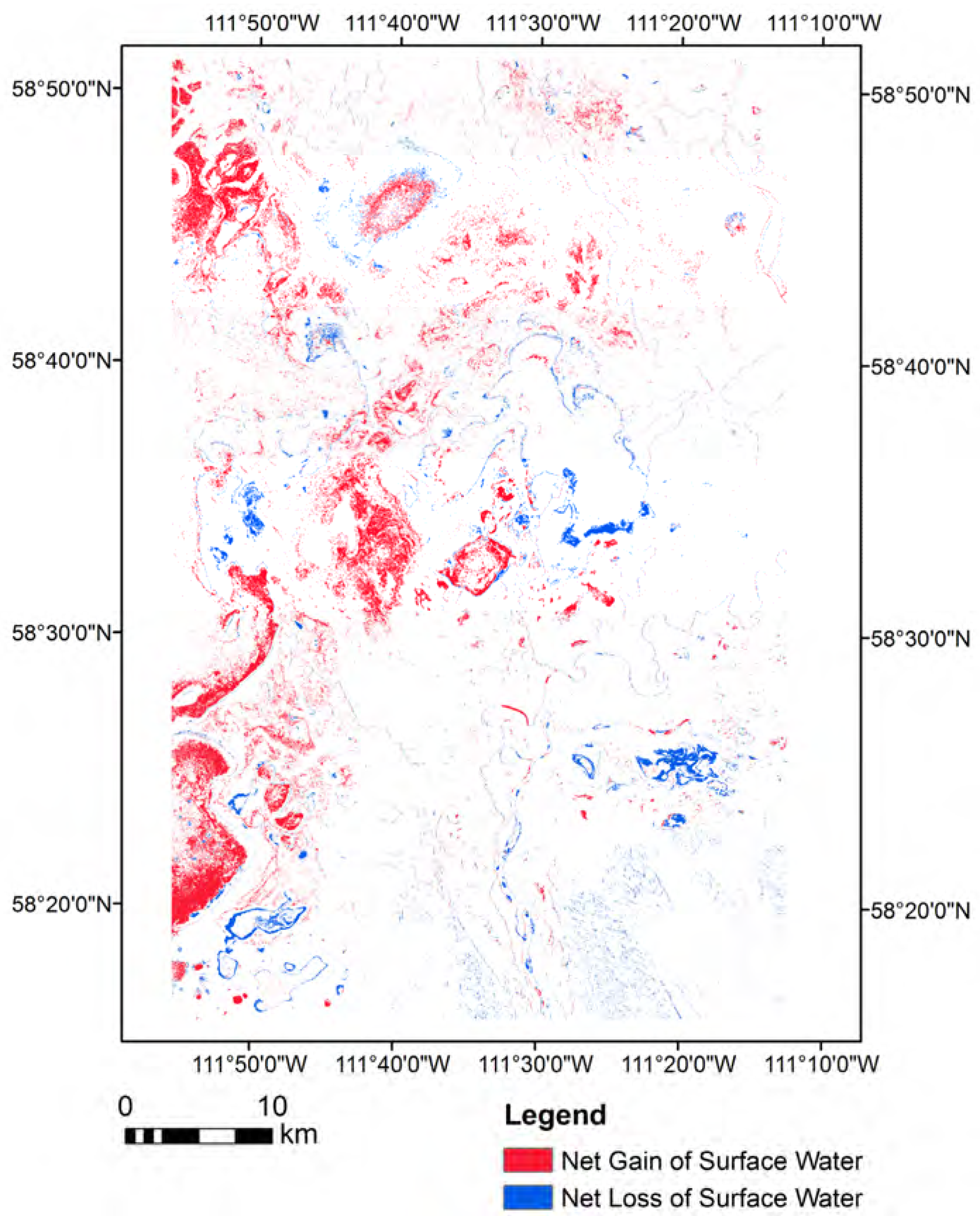
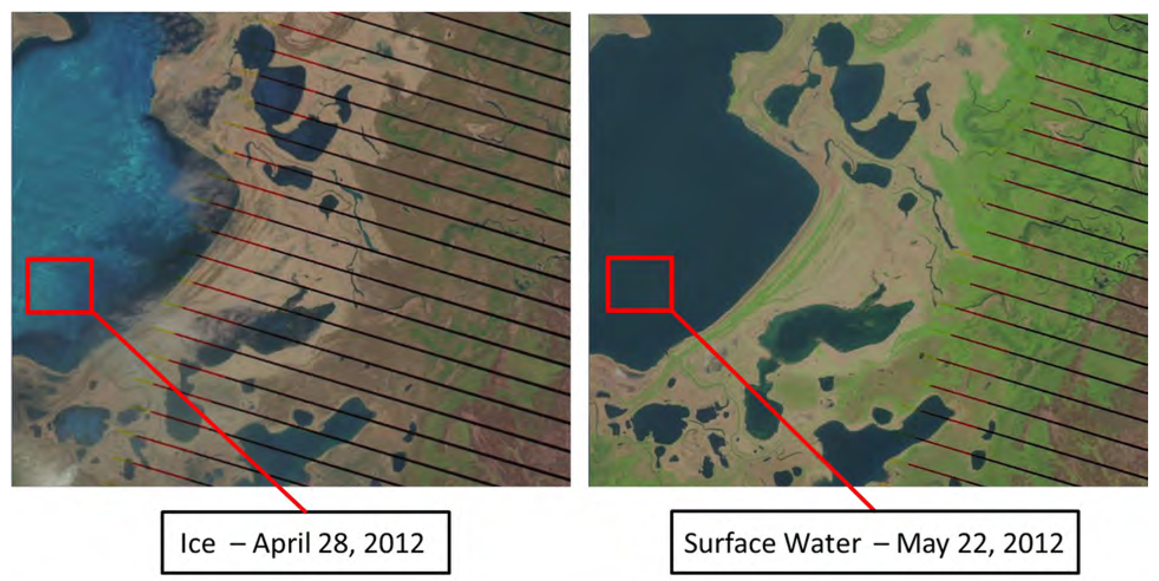
2.1. Case Study—Peace-Athabasca Delta

Surface water thresholding was applied in the Peace-Athabasca Delta (PAD), which is located in northeastern Alberta (58°32′07.46N, 111°40′33.55W). RADARSAT-2 C-band imagery between Lake Claire and Lake Athabasca (Figure 3) were acquired during the 2012 growing season (April to October).
Figure 3. Peace-Athabasca Delta. RADARSAT-2 Ultra-Fine (U2W2) beam acquisition footprint for 2012 (red) and extent of cropped radar-derived surface water product (yellow).
Remotesensing 07 07615 g003

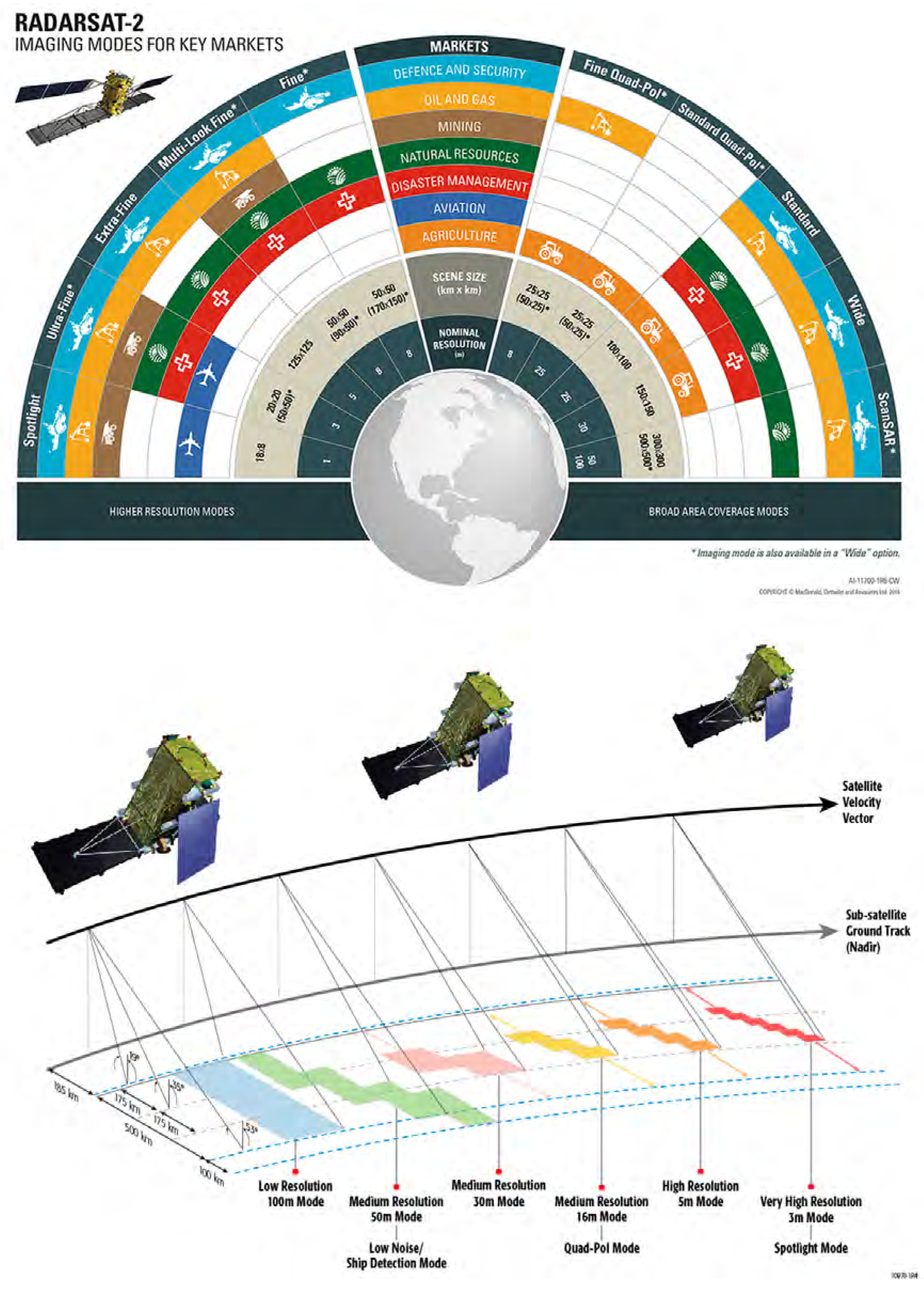
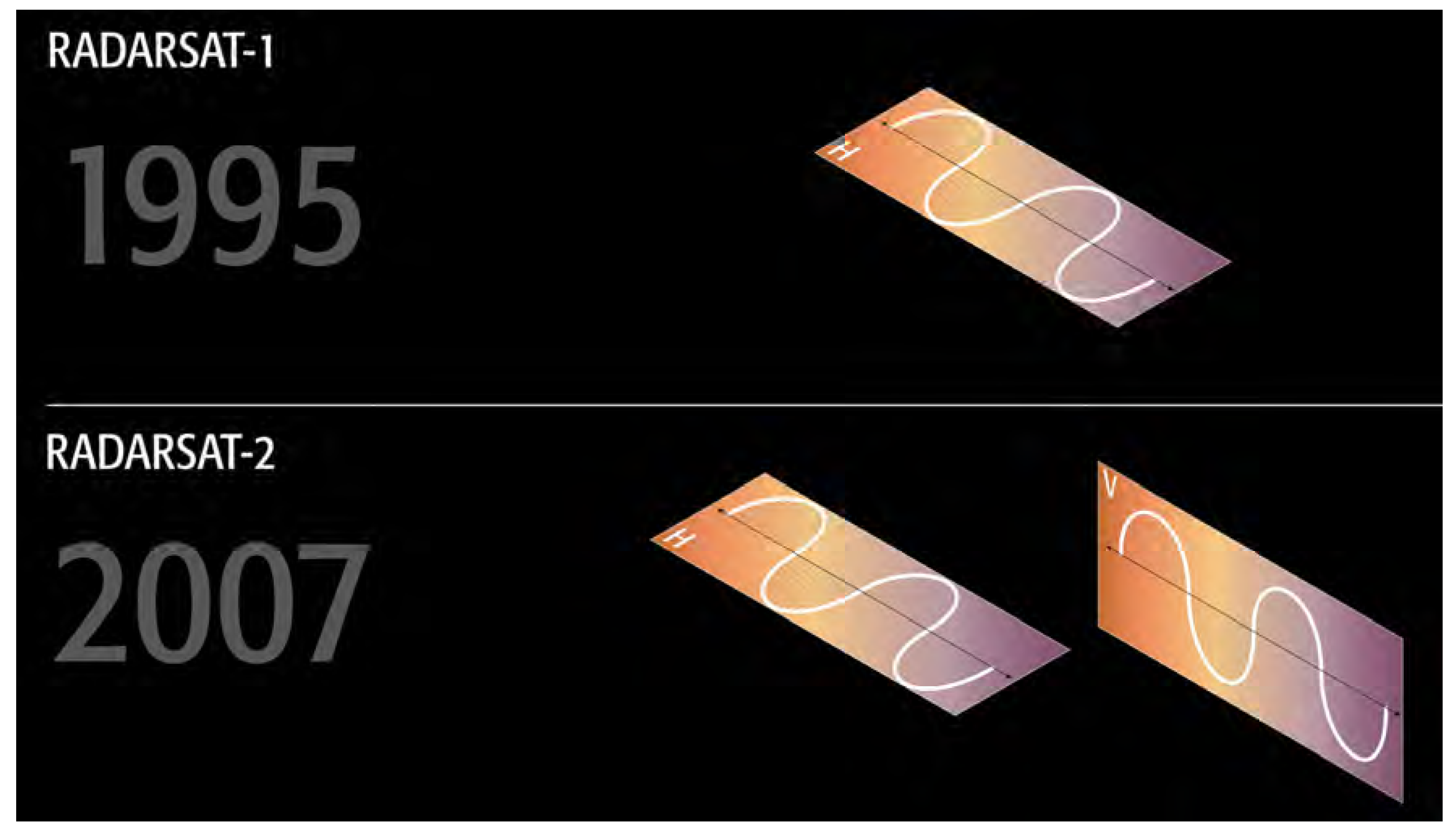
2.2. SAR Data Acquisition and Processing

Two Wide Ultra-Fine (U2W2) mode data frames were captured every 24 days (Table 1). All images were read in as Single Look Complex (SLC; ordered as SLC for other applications, but only the magnitude was used for this application), had an incidence angle of 29.5°–33.0°, a 1.6 × 2.8 m2 resolution, HH polarization, and a swath width of 50 km.
GAMMA SAR remote sensing software [74] was used to process all RADARSAT-2 imagery. A multi-temporal approach was applied to the stack of co-registered SAR intensity images (Table 1) [32]. Granular salt and pepper patterns, referred to as “speckle” in SAR images, occurs when coherent processing of the backscatter returns from consecutive radar pulses [75,76]. We selected a moving weighted function with a filter window size of 5 × 5 pixels to reduce speckle. The result was a filtered intensity image for each image date.
Areas of known surface water were then sampled to determine the range of thresholds (dB) that represented surface water [37]. Surface water thresholds in the PAD for 2012 data ranged from −10 dB to −13 dB. The selection of the surface water threshold was scene specific and was affected by weather conditions, polarization, and incidence angle, and therefore differed among dates to obtain the most accurate results. All images were then orthorectified in GAMMA using 50 m Canadian Digital Elevation Data and a 20 m orthoimagery from the French Satellite Pour l’Observation de la Terre.
Table 1. RADARSAT-2 images acquired over Peace-Athabasca Delta (Lake Claire) for 2012. Note, all RADARSAT-2 images were Single Look Complex (magnitude only used to extract surface water), had an incidence angle of 29.5°–33.0°, a 1.6 × 2.8 m2 spatial resolution, HH polarization, and a swath width of 50 km.
Spring 2012Summer 2012Fall 2012
28 April15 June19 September
22 May9 July13 October
-2 August-
-26 August-
Post editing was done on each image to remove errors of commission. The SAR images were resampled to 20 m and reclassified as surface water (1) and non-water (0). A 20 m SPOT land cover product [77] was used to identify areas of barren ground and sand. A conditional statement was used to reset surface water pixel values with a zero for those areas that overlapped with barren ground or sand.
Ground validation data were not available to verify the results of the surface water maps. We attempted to use Landsat and weather station data to validate our results. We acquired all available Landsat imagery from April to October 2012, where portions of our study site were cloud-free. Three Landsat 7 ETM+ scenes were suitable: 30 April 2012, 1 June 2012, and 21 September 2012. In addition, we used data from the Mildred Lake, Alberta, weather station, approximately 80 km from our study site. We compared mean daily temperature (°C) and total daily precipitation (mm) for each day we produced surface water maps, as well as the monthly average daily mean temperature (°C) and monthly total precipitation (mm).

2.3. Results and Discussion

The results showed that temporal filtering and intensity thresholding was an effective method to map surface water for both large and small water bodies. One advantage of using this approach was that it captured the dynamic changes in the surface water (Figure 4), compared with using static products, such as the 20 m SPOT national land cover product [77] and the National Topographic Data Base (NTDB) water body layers. The net loss or net gain of surface water area from 28 April 2012, to 13 October 2012, provided a spatial snapshot of the water cycle for a particular year and highlighted which areas had an increase or decrease in water extent (Figure 5). It is important to note that the user selection of the threshold approach can introduce uncertainty into how much change in water extent is due to the threshold selection compared to actual environmental changes.
Figure 4. Radar-derived surface water maps from April to August 2012. These images were produced using a thresholding approach and captured the dynamic changes in surface water extent throughout the ice-off period.
Remotesensing 07 07615 g004
Figure 5. These images show the location of net gain (red) and net loss (blue) of water from 28 April 2012, to 13 October 2012, in the Peace-Athabasca Delta.
Remotesensing 07 07615 g005
Landsat and weather station data allowed for some validation of the surface water products. For example, the 30 April 2012, Landsat 7 ETM+ scene showed many of the lakes in the Peace Athabasca Delta were still frozen, which validated that these areas should not be mapped as surface water on the 28 April 2012, RADARSAT-2 image (Figure 6). The same areas in the 1 June 2012, Landsat 7 ETM+ image had melted and could clearly be classified as surface water. This confirmed that the increase in surface that was mapped on the 22 May 2012, RADARSAT-2 image (Figure 6) was reasonable. However, many of the Landsat scenes during the time of this study were too cloudy to use for validation. The weather station data also confirmed that much of the large lakes were still frozen in April 2012, with an average mean monthly temperature of 3.3 °C (Table 2). The average mean monthly temperature rose to 12.2 °C in May (Table 2), providing further evidence that the frozen lakes had melted. July had a high amount of total precipitation (87.6 mm, Table 2), which relates to the expansion of surface water from the 9 July to 2 August images (Figure 4). August was a much drier month with only 33.3 mm of total precipitation (Table 2), causing a decline in surface water by late August (in Figure 4). September was a very wet month (101.1 mm of total precipitation, Table 2), and temperatures were cooling, resulting in an increase in surface water because there was less evapotransporation. The total monthly precipitation for October was less than half compared to September and the monthly mean daily temperature was close to 0 °C, resulting in comparable or a slight increase in extent of surface water. The Mildred Lake, Alberta, weather station (57°02′28.00N, 111°33′32.00W) was the closest to our study area. Although the weather station data helped us interpret changes in water extent over the study period, the station was approximately 80 km away from the Peace Athabasca Delta and may not provide an accurate representation of conditions in the study area.
Figure 6. Landsat scenes used to validate the Peace-Athabasca Delta radar-derived surface water maps. The panel on the left is a Landsat 7 ETM+ scene from 28 April 2012, and the right panel is a Landsat 7 ETM+ scene from 22 May 2012. The red box clearly shows that large portions of the lake were still frozen on 28 April 2012, but had become open water by 22 May 2012.
Remotesensing 07 07615 g006
Table 2. Mildred Lake, Alberta, weather station data. Mean daily temperature (°C) and total precipitation (mm) for the dates of the RADARSAT surface water maps, and monthly average daily mean temperature (°C) and monthly total precipitation (mm).
DateDaily Total Precipitation (mm)Daily Mean Temperature (°C)MonthMonthly Total Precipitation (mm)Monthly Mean Daily Temperature (°C)
28 April 20120.010.0April 201220.63.3
22 May 20120.013.6May 201220.812.2
15 June 20120.013.3June 201258.016.9
9 July 20120.025.3July 201287.620.6
2 August 20125.717.2August 201233.318.3
26 August 20120.017.2September 2012101.113.4
19 September 20120.312.5October 201244.40.7
13 October 20120.01.5
Grey-level thresholding has been proven to be a simple and effective way to map surface water with SAR data [33,37]. However, the user must consider beam mode, polarization and ancillary sources of data for post-editing to obtain an accurate result. The HH polarization generally is better able to separate land from water under calm water conditions because open water results in less scattering compared to the HV or VV polarization and is less sensitive to capillary waves created from wind [78]. Therefore, the differences in backscatter responses between land and water are the greatest in the HH polarization [46,70,79,80,81]. In circumstances where high wind or waves are present the HV polarization can better map open water because the backscatter is more independent of surface roughness [82] and largely independent of incidence angle and wind direction [78]. When mapping surface water, we recommend ordering the SAR data as dual-polarized to enable the user to select the most appropriate polarization for the wind conditions present at the time of data acquisition. The user also must do some post-classification editing to remove errors of omission and commission. Ancillary sources of information, such as digital elevation layers, ground truth data, and a land cover mask, can aid in the editing. Ordering the appropriate SAR data and doing post-editing with appropriate ancillary data will help ensure accurate surface water mapping.

3. Flooded Vegetation

Open water and flooded vegetation both need to be mapped to accurately represent the extent of a wetland. The long wavelengths associated with SAR systems allow the signals to penetrate vegetation canopies to map underlying emergent herbaceous and woody wetland vegetation via double-bounce backscatter [34,57,83,84,85]. The longer the wavelength, the deeper the penetration through the vegetation canopy. P-band radar signals (30−100 cm wavelengths) penetrate nearly all canopies; L-band signals (15−30 cm) penetrates many canopies; and C-band (3.75–7.5 cm) and X-band (2.4–3.75 cm) signals only penetrate open canopies or denser canopies during leaf-off conditions or if the overstory is dead.
Single polarization SAR satellites, which provide only amplitude data (e.g., RADARSAT-1), are not as efficient in mapping flooded vegetation because the radar backscatter cannot be decomposed with only one intensity channel. However, when polarimetric decompositions are applied using fully polarimetric SAR, features like flooded vegetation can be identified and classified [86]. Many polarimetric decomposition approaches have been developed, including the Cloude-Pottier, Freeman-Durden, Van Zyl, Touzi, and m-χ methods [86,87,88,89,90]. The Freeman-Durden decomposition is a physically based model that estimates the amount of surface, double-bounce, and volume scattering response contributing to the total backscatter from each pixel [88]. The m-χ decomposition estimates the received Stokes Vectors and converts them to the Poincaré features m and χ [90]. We describe a case study using the Freeman-Durden decomposition, for which past research has demonstrated its ability for mapping flooded vegetation and wetlands [37,86,88], and the m-χ decomposition. Both methods output a three-channel image with estimates of surface, double-bounce and volume scattering, allowing for easy comparison of outputs. Comprehensive descriptions of these decompositions are provided by Freeman and Durden [88] and Raney et al. [90].

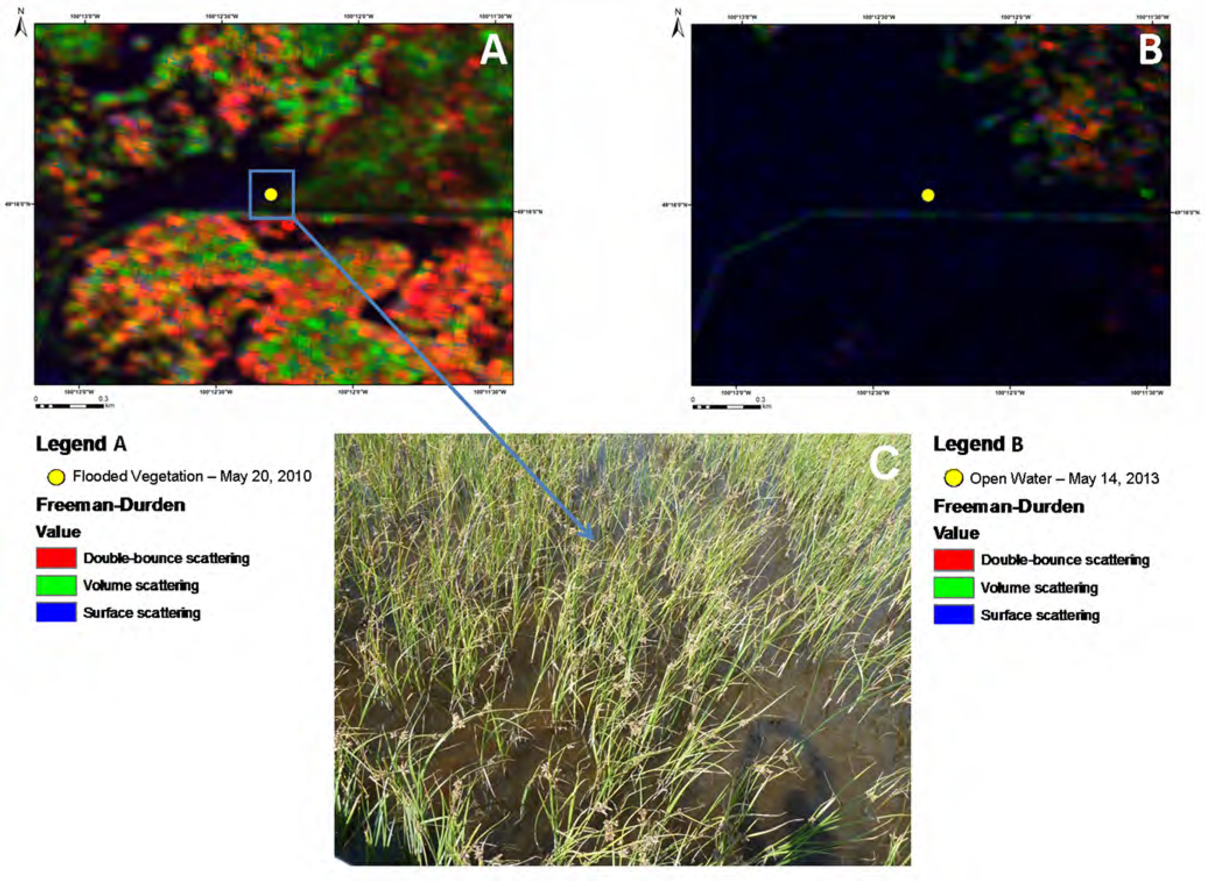
3.1. Case Study—Whitewater Lake

Whitewater Lake (49°15′05.46N, 100°12′18.90W) is located in southwestern Manitoba, between Boissevain and Deloriane (Figure 7). This lake is recognized as a Canadian Important Bird Area of global significance, providing habitat for more than 110 species of birds, as well as other wildlife. Shallow saline wetland, sedge meadows, and mixed-grass prairie are all found within the Whitewater Lake Basin.
Figure 7. Whitewater Lake, Manitoba. All field data points were collected inside the red square.
Remotesensing 07 07615 g007

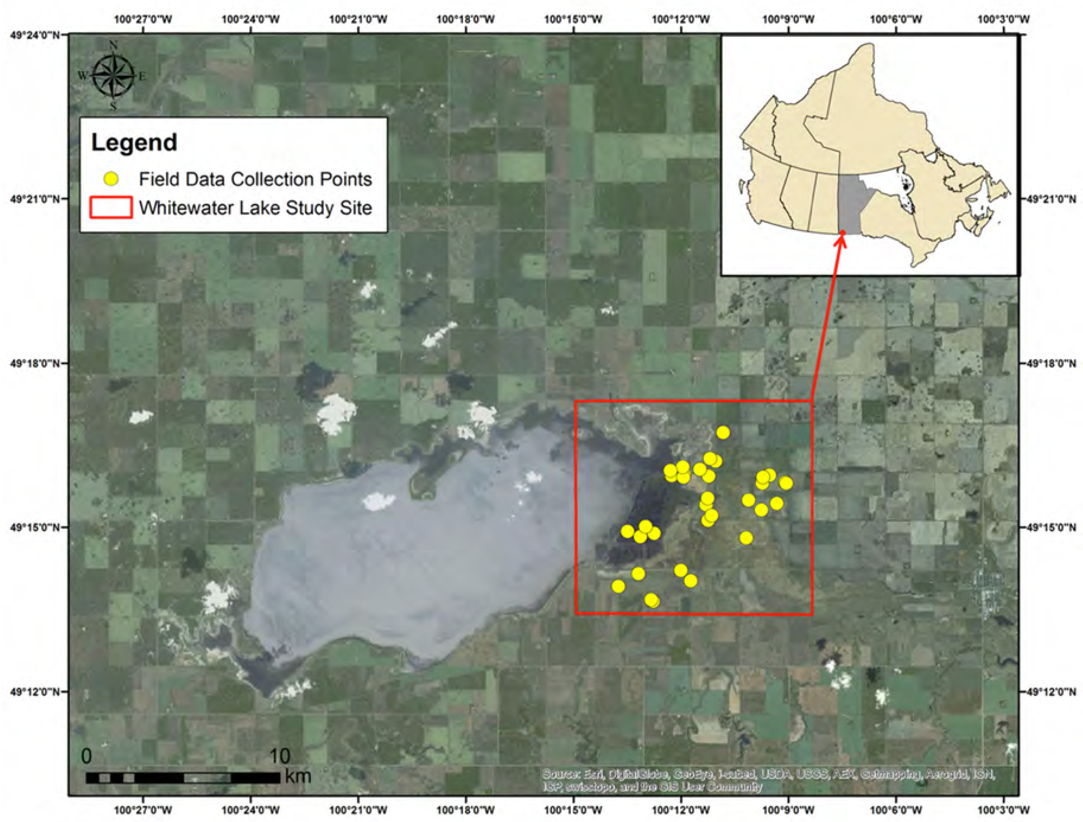
3.2. Data Acquisition and Processing

RADARSAT-2 images were acquired throughout the growing season for 2010, 2012, and 2013 (Table 3). All images were Fine Quad-Pol (FQ16) mode with a nominal resolution of 5.2 × 7.6 m2 and an incident angle of 35.4°–37.0°.
Ducks Unlimited Canada (DUC) independently selected 31 field points that had undergone a land cover change during or between years included in this research. DUC recorded the land cover type and date from the earlier image, the new land cover type and date from the later image, observational notes, and field photos.
All image processing for the Freeman-Durden decomposition products was done using Geomatica 10.3.2 [91]. A 5 × 5 pixel boxcar filter (which used local averaging to increase the effective number of looks) was applied to remove speckle. The Freeman-Durden decomposition was then derived to separate the total power of each pixel into surface, double-bounce, and volume scattering. The output was a three channel image corresponding to the power of each of the three scattering mechanisms.
Table 3. RADARSAT-2 images acquired over Whitewater Lake, Manitoba, in the spring, summer, and fall of 2010, 2012, and 2013. These images were used to determine if simulated compact polarimetric data could be used to map changes in wetlands within a growing season and between years. Note, all RADARSAT-2 images in this flooded vegetation analysis were FQ16 mode with an incidence angle of 35.4°−37.0° and a nominal resolution of 5.2 × 7.6 m2.
201020122013
6 May19 May14 May
30 May12 June7 June
17 July6 July1 July
3 September16 September18 August
21 October10 October11 September
5 October
The m-χ decompositions were processed using software to simulate compact polarimetry, which was created at the Canada Centre for Mapping and Earth Observation. The software ingests fully polarimetric SLC imagery and simulates compact polarimetry data. A 30 m resolution, −25 dB noise floor and a 5 × 5 pixel averaging window were applied, as these parameters most closely resemble the parameters of RCM data.
All images were orthorectified after all polarimetric analyses were completed because the orthorectification process can degrade the phase information contained within the polarimetric images [92]. Both the Freeman-Durden and m-χ decompositions were orthorectified using Geomatica’s 10.3.2 Orthoengine. The rational function option, which uses the ephemeris data provided by MacDonald, Dettwiler and Associates for each RADARSAT-2 image, was applied instead of collecting ground control points. All images were expected to have an error less than half a meter. In addition, a 50-m Canadian Digital Elevation Data Digital Elevation Model (50 m resolution), cubic convolution pixel resampling, and sigma naught calibration were used in all orthorectifications. Sigma naught is the normalized measure of the backscatter from the feature being sensed, also known as the backscatter coefficient [93].
To determine if the Freeman-Durden and m-χ decompositions could be used to accurately map flooded vegetation, the 31 points collected by DUC representing land cover change were overlaid on the decompositions. A visual assessment was done to verify if the land cover change (for example open water becoming flooded vegetation) observed by DUC was also visible as a change in backscatter in the decompositions, in which case changes in backscatter could be used to map areas of flooded vegetation. We used a scale from 1 to 3 to rank the utility of the decompositions to map change between land cover classes. A “3” represented a complete separation between two land cover classes; a “2” represented moderate separation between classes; and a “1” represented little separation between classes.

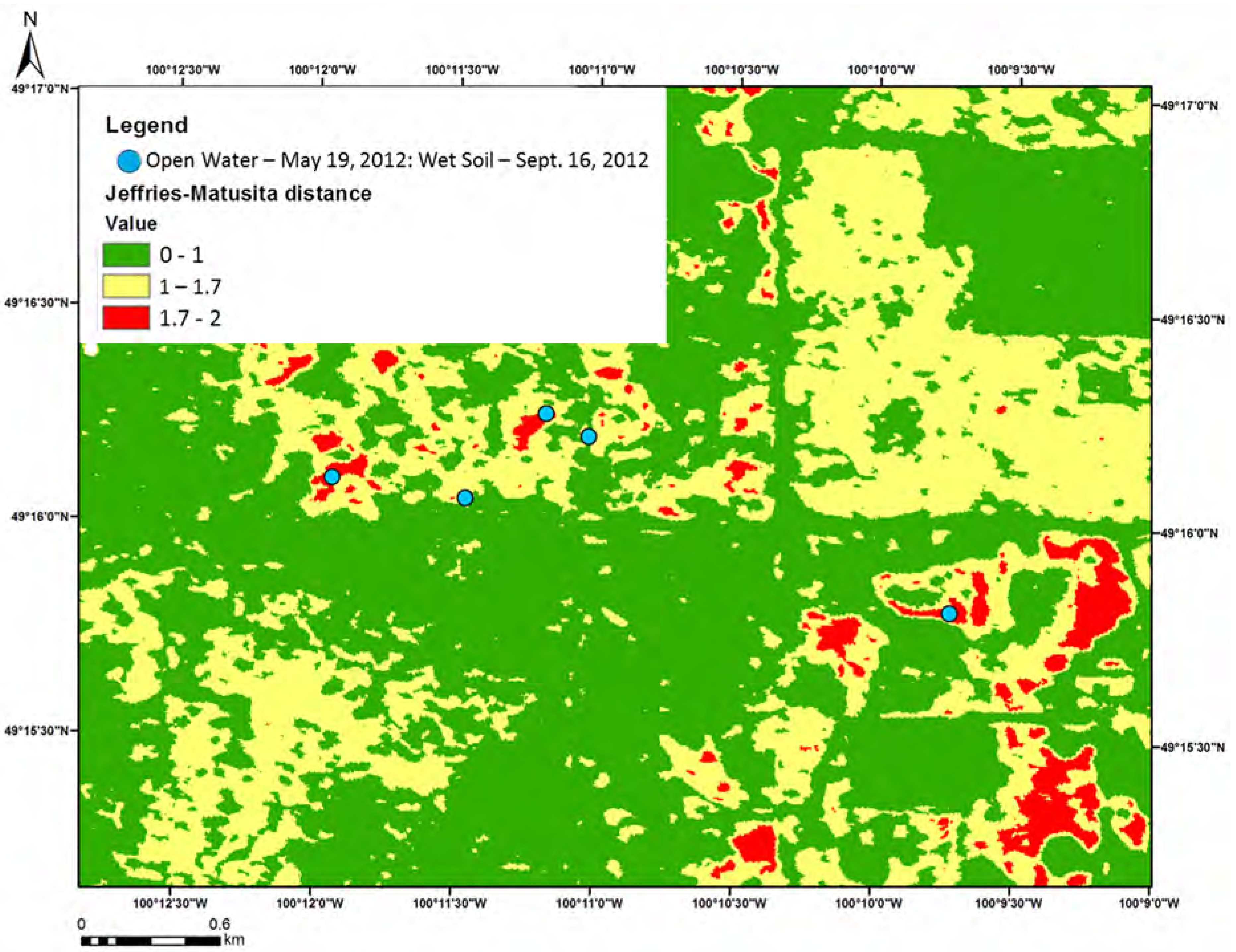
3.3. Results and Discussion

Both the Freeman-Durden and m-χ decompositions were effective for mapping changes between different land cover classes within a wetland, both annually and inter-annually. The Freeman-Durden decomposition had a high accuracy rate for identifying land cover changes for all combinations in this study (Table 4). The flooded vegetation land cover was usually dominated by double-bounce backscatter, whereas open water had specular backscattering, upland vegetation had volume backscattering, and areas of wet soil were dominated by surface scattering. These results were consistent with research by Ramsey [94] that concluded flooded mangroves could be classified from non-flooded mangroves because the former was largely a double-bounce backscatter response and the later a volume backscatter response in L-HH data. These distinctly different backscattering responses made the transition from land cover classes easily detectable. For example, upland vegetation in the spring of 2010 was clearly classified as having a large amount of volume scattering, and in the summer of 2013 the same area was inundated by open water and exhibited specular backscattering, appearing dark on the image because very little backscatter was returned to the satellite (Figure 8). However, there were a few areas where the Freeman-Durden method was ineffective at identifying land cover change between open water and flooded vegetation because the patch sizes were small and were therefore given a rank of 1 or 2. Small, dispersed patches of flooded vegetation (<5 × 5 m2) do not return the strong double-bounce backscatter typically associated with flooded vegetation. Vegetation that is short or patchy can have a backscatter more similar to water (Figure 9). Alternatively, a study in Kenya with C-HH imagery found that flooded emergent grasses had a similar backscatter response to non-flooded grasses [95]. The confusion in identifying the change in land cover from upland to open water likely was a result of wind causing waves in the water and, consequently, a lot more surface scattering. When all land cover class transitions were considered, the Freeman-Durden results had an overall accuracy rate of 89%.
Table 4. The results from a visual assessment to determine how accurate the Freeman-Durden and m-χ decompositions were at classifying changes between land cover classes.
Land Cover, Time 1Land Cover, Time 2% Correct Change Detection Freeman-Durden% Correct Change Detection m-χ
Annually
Wet soilOpen water100%100%
UplandOpen water100%100%
UplandFlooded vegetation80%80%
Open waterFlooded vegetation87%69%
Seasonally
Wet soilOpen water73%80%
UplandOpen water
UplandFlooded vegetation67%67%
Open waterFlooded vegetation100%67%
Overall
AnyAny89%81%
Figure 8. This image shows the transition from upland vegetated areas on 30 May 2010 (A,B), to open water on 25 July 2013 (C,D). Images (A) and (C) were produced from the Freeman-Durden decomposition and images (B) and (D) from the m-χ decomposition. Both decompositions were able to clearly map the change from upland vegetation to open water because the upland areas had a strong volume scattering response and the open water returned very little backscatter to the satellite and, thus, appeared black.
Remotesensing 07 07615 g008
Consistent with the Freeman-Durden decomposition, m-χ was able to separate many land cover transitions with a high accuracy rate (Table 4). For example, when upland vegetated areas in the spring of 2010 became open water in the summer of 2013, the m-χ decomposition output clearly mapped the changes from volume scattering to specular scattering (Figure 8). Nevertheless, the m-χ decomposition did not map changes from open water to flooded vegetation as well as the Freeman-Durden decomposition. This was because the double-bounce backscattering was not as visible in the m-χ decomposition. In many samples, the m-χ decomposition gave a mixed backscatter response in areas of flooded vegetation. However, the m-χ decomposition had a slightly higher accuracy rate than the Freeman-Durden decomposition when used to map changes from wet soil to open water within a season. This was because a few samples were a mix of mud and vegetation, which returned some double-bounce backscatter in the Freeman-Durden decomposition.
Figure 9. This figure shows the results of the Freeman-Durden decomposition from 30 May 2010 (A); and 14 May 2013 (B). The yellow point is a location that was flooded vegetation on 30 May 2010, but changed to open water on 14 May 2013. The Freeman-Durden decomposition was not able to map this specific change because the flooded vegetation was short (C), thus there was not a strong double-bounce backscatter returned to the satellite; rather the return was a specular backscatter similar to open water.
Remotesensing 07 07615 g009
Although both the Freeman-Durden and the m-χ decompositions successfully mapped changes in land cover types, the Freeman-Durden decomposition had a better overall accuracy rate. This was not surprising because the simulated compact polarimetry data had a noise floor of −25 db, compared to −35 db for the fully polarimetric data. In addition fully polarimetric SARs capture more information (4 × 4 matrix) compared to compact polarimetric SAR’s (2 × 2 matrix). Moreover, when the transmission of a field has a linearly polarized component it will cause uncertainties or omission when classifying dihedral backscatter [96]. Circular polarization transmission is the best way to prevent the rotation of a linearly polarized wave as it transmits through the ionosphere, but some omission may still occur [97]. Therefore, some features will not be as visible in the simulated compact polarimetry data because they are too faint and do not exceed the noise floor.
Although in some examples both decompositions were given a rating of 2 because there was a mixed backscatter response, this does not necessarily indicate a poor ability to map land cover change. These results may indicate that the targets were heterogeneous, such as open water with emergent macrophytes. This information could be used as an indicator of the health of a wetland, for example, biomass within a wetland. The amount of volume and double-bounce scattering can be an indicator of vegetation density. However, further research and development is needed to quantify not only the difference in vegetation versus no vegetation, but also how different resolutions, bands, and angles of radar reflect off different vegetation types, densities, and heights. It has been suggested that C-band imagery should be used when trying to map leaf shape and that L-band is more accurate for measuring aboveground biomass and stand height [98]. Other research has demonstrated that a multi-temporal and multi-incidence angle was the best approach, with steep incidence angles for mapping wetlands and large incidence angles for detecting open water from land [99,100,101].

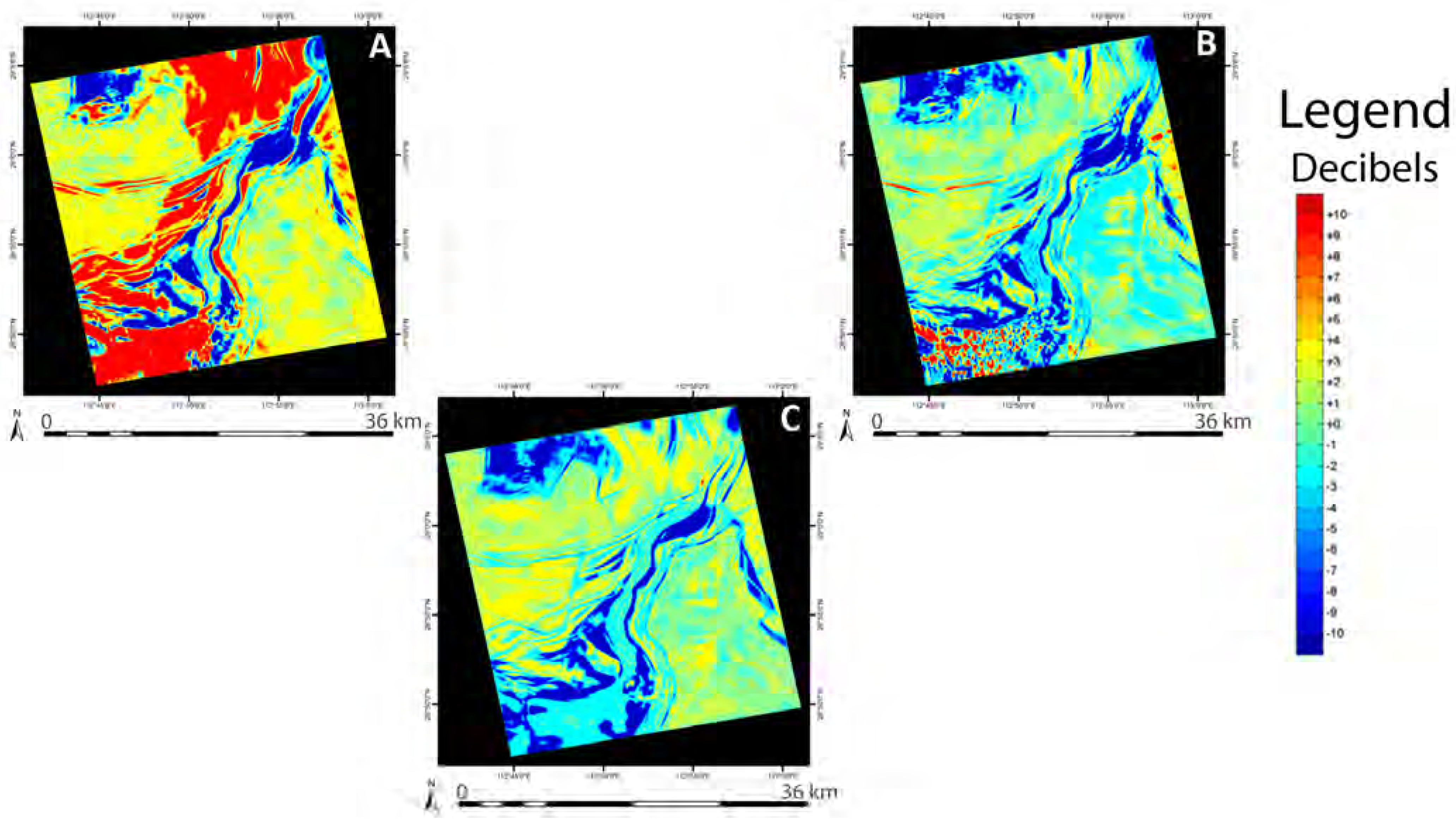
4. Curvelet-Based Change Detection for Mapping Flooded Vegetation

More recently a Curvelet-based approach for detecting changes in flooded vegetation has been used [49,102,103]. This technique was developed by Schmitt et al. [104] and can be used to map changes between SAR images while at the same time suppressing speckle noise, which can be problematic in SAR imagery. This approach could be used as a way to enhance polarimetric decompositions and temporal changes between polarimetric channels.
This methodology was originally designed for disaster management with single polarimetric SAR, but was later adapted to use in polarimetric decompositions. This approach differs from others in that it compares whole structures found in the image rather than individual pixel values. The first step is to apply the Curvelet transform [105] on each input image separately. This technique detects elongate structures – in general, “lines” like the course of a river – in the images and then converts the images to the so-called Curvelet-coefficient domain, where each coefficient stands for a certain “line” in the image. Comparing the Curvelet coefficients of two images consequently means comparing structures apparent in the two input images, which enables a very stable and quasi-noise-free change detection. For instance, the change of an isolated pixel value—mainly induced by noise influence only—will not be detected. But, the consistent change of several neighboring pixels will produce a new structure and, therefore, it is detected by the Curvelet-based change detection approach. The change of the water level, for example, mostly produces a shift of the shoreline, i.e., the Curvelets describing the transition from land to water along the shoreline will also change, which becomes evident in the comparison of their coefficients. The finest scale considered in the change detection refers to a neighborhood of approximately 3 × 3 pixels [104].
The direct mathematical description of the structures in an image opens to door to structure amplification and, thus, image enhancement because manipulating the Curvelet coefficient is equal to manipulating the structures instead of single pixel values [106]. For example, low Curvelet coefficient amplitudes generally indicate very weak structures and are mostly related to noise, e.g., of low backscattering targets like open water. This noise contribution can easily be deleted by converting the corresponding coefficients to zero before the image reconstruction. In addition coefficients with a higher value, which are usually related to intense structures like the shoreline or the border between flooded vegetation and open water, are weighted by using a special function, which retains the values of the strong structures while slightly lowering the values for minor structures [104] to suppress artifacts common to all alternative image representations. The same image enhancement can be used for individual SAR images as well as for the difference between images. In practice, the image difference is calculated in the complex Curvelet coefficient domain, then the differential coefficients are weighted, and finally the enhanced difference image is transformed back to the image domain [102]. For more details on how the Curvelet-based change detection method is calculated refer to [49,62,63,102,103,104].
To apply the change detection algorithm to polarimetric decompositions all three decomposition channels, representing three independent intensity measures, can be introduced as independent layers. Whereas an increase or decrease in intensity only (without changing the scattering mechanism) will appear adequately in all three channels (compared with the change of the dielectric constant from differences in soil moisture, for example), the change of the scattering mechanism will be described by a very special behavior in the polarimetric channels [49]: an increase in the volume component directly refers to growth in vegetation height; a higher surface component indicates the appearance of a relatively smooth target (e.g., grassland formerly covered by water); and an increase in the double-bounce component traces the expanded extent of flooded vegetation along the river. Hence, this technique not only detects changes, but allows the user to interpret the changes with respect to temporal variations in the land cover.

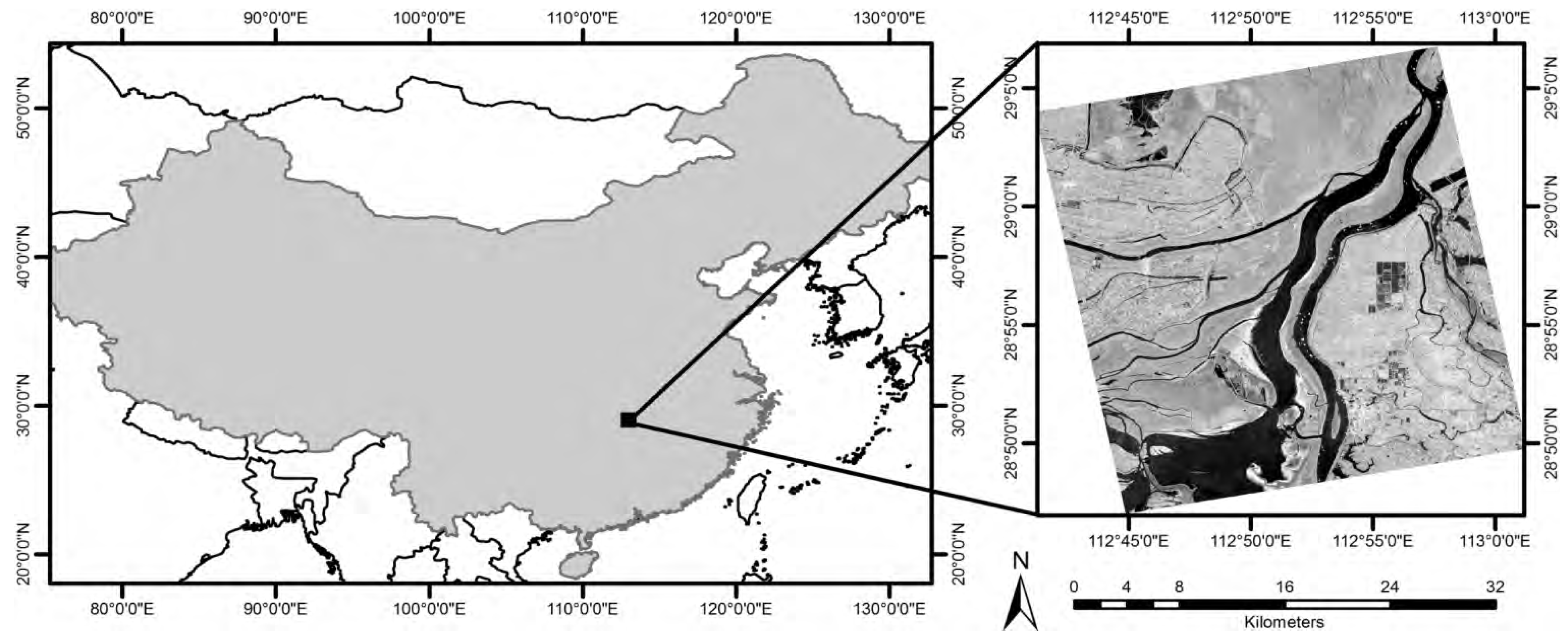
4.1. Case Study—Dong Ting Lake

Dong Ting Lake is located in Hunan Province (28°53′22.11N, 112°40′01.33W) (Figure 10). It is the second largest lake in China and is a flood basin within the Yangtze River. The size of Dong Ting Lake can change quite dramatically within a season. For example, it can be as large as 2691 km2 during an annual flood event and as small as 710 km2 during dry conditions [107].
Figure 10. The location of the Dong Ting Lake test site in China.
Remotesensing 07 07615 g010

4.2. Data Acquisition and Processing

Two RADARSAT-2 fully polarimetric scenes (FQ16) were acquired over Dong Ting Lake in 2008. Both images had an incidence angle of 35.4°−37.0° and a nominal resolution of 5.2 × 7.6 m2. An image with lower water levels (6 June 2008) and an image with higher water levels (17 August 2008) were selected for change detection. The Freeman-Durden decomposition was used as input into the Curvelet-based change detection method to determine if this technique could detect change between the three different types of backscatter produced in the Freeman-Durden decomposition.

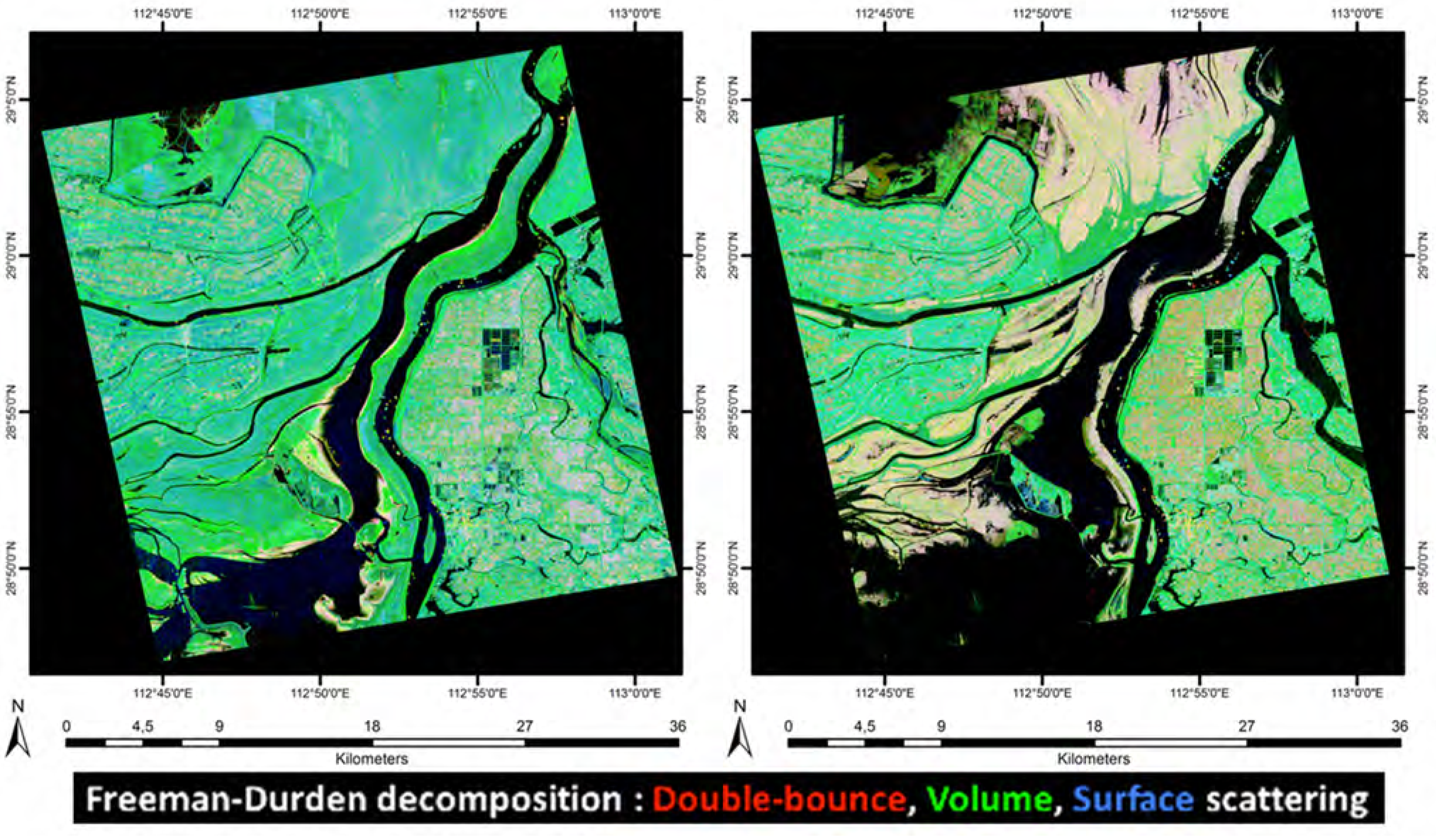
4.3. Results and Discussion

When the Freeman-Durden decompositions were compared using the Curvelet-based change detection, the results showed that the Curvelet-based change detection could be used to map changes in the double-bounce, volume and surface scattering in a smooth, noise-free manner while still preserving detail. When comparing the Freeman-Durden decompositions of the single images in Figure 11, the dominance of the volume scattering component (green) is highly visible. Apart from that, a change from surface scattering (the bluish fields in the upper part of the 6 June 2008, image) to double-bounce (the fields now turned to orange or even red in the 17 August 2008, image) can clearly be distinguished. The dilation of the water surface (black) from June to August is likewise apparent.
Figure 11. The Freeman-Durden decompositions derived from the 6 June 2008, and 17 August 2008, RADARSAT-2 acquisitions.
Remotesensing 07 07615 g011
Figure 12 illustrates the results of the Curvelet-based change detection method. The strongest changes can be found in the double-bounce component, reaching more than 10 decibels in gains or losses of double-bounce response. The lowest changes are reported in the volume component. Combining all three difference images enables a simple change characterization. Similar changes captured in all three components indicate a change in the image intensity, i.e., a change in the open water surface. Changes only apparent in one channel indicate an increase or decrease of a special scattering mechanism. Examining the fields in the upper part of the image, minor changes are shown both in the volume and the surface component, but very strong changes in the double-bounce component are evident. This means that new very strong double-bounce scatter components are added while the surface and volume scattering remain constant. In regard to the landscape, these fields are flooded.
Figure 12. The Curvelet-based approach was applied to RADARSAT-2 acquisitions for 6 June 2008, and 17 August 2008, to highlight changes in the Freeman-Durden components: double-bounce scattering (A); surface scattering (B); and volume scattering (C).
Remotesensing 07 07615 g012
These results highlight the possibility for the Curvelet-based change detection to be used with polarimetric SAR data. Wetland land cover change was detected using the Freeman-Durden decomposition as input to the Curvelet-based method. These results are consistent with another study, which applied the same approach using the Freeman-Durden and the Normalized Kennaugh elements to locate changes in flooded vegetation [102]. Though first efforts to validate the changes observed by the Curvelet-based change detection method are reported in Schmitt et al. [104], the validation with regards to wetland monitoring is still challenging and should be extended to a variety of test sites in the future using auxiliary data from other sources like unmanned aerial vehicles.

5. Wishart-Chernoff Distance

The ability to focus and prioritize monitoring efforts is often a difficult task, but necessary in a time when the environment, including wetlands, is being altered at an alarming rate and monitoring budgets are shrinking. Having a tool to identify areas that have undergone the most change over a time period is an invaluable first step in monitoring wetlands. Whitewater Lake, Manitoba (see Figure 6), with the available SAR data shown in Table 3 was used as a test site for change detection within wetlands. The Wishart-Chernoff distance, derived and proposed by Dabboor et al. [108], was used for pixel-based polarimetric change detection mapping. As analytically presented [108], the Wishart-Chernoff distance is a probabilistic matrix distance measure that can estimate the similarity between two complex Wishart distributions and, thus, be used for applications involving full and compact polarimetric SAR data imagery. The Wishart-Chernoff distance is a symmetric positive matrix distance that can be used in a wide range of applications, such as agglomerative clustering [108,109] and change detection applications [110]. The same image dates used for mapping flooded vegetation in the Whitewater Lake example were used in the Wishart-Chernoff Distance analysis (see Table 3). Data were geo-referenced and co-registered with accuracy to better than one pixel. Images were compared on a pixel-by-pixel basis by calculating within a moving window (3 × 3) the Wishart-Chernoff distance between corresponding pixels. High values of the Wishart-Chernoff distance indicated significant changes in the study area between the acquisitions dates of the images.

5.1. Case Study—Whitewater Lake

Whitewater Lake, Manitoba, was used as the location to test the Wishart-Chernoff Distance methodology (see Figure 7).

5.2. SAR Data Acquisition

The same image dates used for the flooded vegetation example were used in the Wishart-Chernoff Distance analysis (see Table 3).

5.3. Results and Discussion

To analyze the detected changes within the regions of the Whitewater Lake, a specific range of pixel values must be defined tobe able to map the changes. Thus, the calculated Wishart-Chernoff distance values (DWC) were expressed in terms of the Jeffries-Matusita distance (DJM) as follow: DJM = 2(1 − e D W c ). The advantage here is that the Jeffries-Matusita distance takes values between 0 and 2. High Jeffries-Matusita distance values (high Wishart-Chernoff distance values) close to 2.0 indicate changes and low distance values (below 1.0) indicate little or no changes [111]. We used a threshold value of 1.7 to discriminate between large changes (DJM > 1.7) and moderate changes (1 < DJM < 1.7) [112].
The Wishart-Chernoff Distance showed promising results when identifying areas of moderate and high change within a wetland. When we compared the areas that DUC had independently identified as having undergone a change in land cover based on field photos and field data collection, we verified that the Wishart-Chernoff Distance method had identified these same locations as either areas of high or moderate change. For example, areas of open water on 19 May 2012, that had become wet soil by 16 September 2012, were flagged as high or moderate change with the Wishart-Chernoff Distance method (Figure 13). Similar results were found annually for land cover change between open water and flooded vegetation, open water and upland, and upland and flooded vegetation.
Figure 13. Areas of open water on 19 May 2012, that became wet soil by 16 September 2012, are indicated by the blue dots. The background image is the Wishart-Chernoff Distance calculated using fully polarimetric data from the two dates. Red polygons are areas estimated to have high amounts of change; yellow areas signify moderate change; and green areas signify little or no change.
Remotesensing 07 07615 g013
The Wishart-Chernoff Distance change detection shows encouraging results as a tool to flag areas of high and moderate change within wetlands. It could be used to first locate areas of high change, after which polarimetric decompositions could be applied to characterize the type of change. Further research is needed to develop the methodology and to confirm the results.

6. Conclusions

Analysis of Synthetic Aperture Radar Imagery data is an excellent approach for mapping and monitoring changes within a wetland. The ability of SAR data to be acquired at night and in a variety of weather conditions makes it a reliable and consistent source of information. Past studies have demonstrated that grey-level thresholding is an effective way to map surface water. Polarimetric decompositions like the Freeman-Durden and m-χ approaches can be used to map flooded vegetation, and the curvelet-based change detection can further enhance the detection of flooded vegetation by reducing speckle and other forms of noise. Finally, the Wishart-Chernoff Distance change detection approach could be used to flag areas of change prior to implementing polarimetric decompositions to characterize these changes. To be able to monitor the status of wetlands on a frequent basis and capture the dynamic changes both seasonally and annually we recommend SAR as the primary source of imagery, supported by other data sources such as lidar, thermal, and optical imagery, where feasible.

Acknowledgments

This research project was supported by the RSS program at ESS/CCRS and the CSA through the RCM-CCD funding. Thanks to Junhua Li, Don Raymond and two anonymous reviewers for critical comments on the manuscript. We would also like to thank the guest editor Alisa Gallant.

Author Contributions

Brian Brisco was one of the project managers for all case studies in this paper. He helped develop all research methods, and assisted in the analysis of all results. Mohammed Dabboor led the research on the Wishart-Chernoff distance. Mohammed worked with Lori White and Brian Brisco to guide them in implementing the Wishart-Chernoff distance approach in Whitewater Lake, Manitoba. Mohammed assisted in the interpretation of the results and the writing of the Wishart-Chernoff Distance case study. Andreas Schmitt together with Brian Brisco led the curvelet-based change detection research. He also helped write the curvelet-based change detection for mapping flooded vegetation section of this paper. Andrew Pratt helped choose the study site, collect the field data, and analyze and interpret the results for the flooded vegetation case study. Andrew also contributed to the writing of the flooded vegetation case study and the introduction of the paper.

Conflicts of Interest

The authors declare no conflict of interest.

References

  1. Vymazal, J. Constructed wetlands for wastewater treatment. Ecol. Eng. 2005, 25, 475–477. [Google Scholar] [CrossRef]
  2. Mitsch, W.; Gosselink, J. The value of wetlands: Importance of scale and landscape setting. Ecol. Econ. 2000, 35, 25–33. [Google Scholar] [CrossRef]
  3. Anderson, B.C.; Watt, W.E.; Marsalek, J. Critical issues for stormwater ponds: Learning from a decade of research. Water Sci. Technol. 2002, 45, 277–283. [Google Scholar] [PubMed]
  4. Gedan, K.B.; Kirwan, M.L.; Wolanski, E; Barbier, E.B.; Silliman, B.R. The present and future role of coastal vegetation in protecting shorelines: Answering recent challenges to the paradigm. Clim. Chang. 2010, 106, 7–29. [Google Scholar] [CrossRef]
  5. Cox, D.D. A Naturalist’s Guide to Wetland Plants: An Ecology for Eastern North America; Syracuse University Press: Syracuse, NY, USA, 2002; p. 10. [Google Scholar]
  6. Natural Resources Canada. Sensitivity of Peatlands to Climate Change. Available online: http://atlas.nrcan.gc.ca/site/english/maps/climatechange/potentialimpacts/sensitivitypeatlands/1 (accessed on 5 August 2014).
  7. IUCN. 2007 IUCN Red List of Threatened Species. Available online: www.iucnredlist.org (accessed on 21 December 2014).
  8. Prigent, C.; Papa, F.; Aires, F.; Jimenez, C.; Rossow, W.B.; Matthews, E. Changes in land surface water dynamics since the 1990s and relation to population pressure. Geophys. Res. Lett. 2012, 39, L08403. [Google Scholar] [CrossRef]
  9. Ferrati, R.; Canziani, G.A.; Moreno, D.R. Estero del Ibera: Hydrometeorological and hydrological characterization. Ecol. Model. 2005, 18, 3–15. [Google Scholar] [CrossRef]
  10. Scientific and Technical Review Panel of the Ramsar Convention on Wetlands. New guidelines for management planning for Ramsar sites and other wetlands. “Wetlands: water. Life, and culture”. In Proceedings of 8th Meeting of the Conference of the Contracting Parties to the Convention on Wetlands (Ramsar, Iran, 1971), Valencia, Spain, 18–26 November 2002.
  11. United States Environmental Protection Agency (US-EPA). Wetlands Treatment Database (North American Wetlands for Water Quality Treatment Database); US-EPA: Washington, DC, USA, 1994.
  12. United States Environmental Protection Agency (US-EPA). Constructed Wetlands for Wastewater Treatment and Wildlife Habitat: 17 Case Studies; US-EPA: Washington, DC, USA, 1993. [Google Scholar]
  13. Environment Canada. Water and Climate Change. Available online: http://www.ec.gc.ca/eau-water/default.asp?lang=En&n=3E75BC40-1 (accessed on 30 December 2014).
  14. Root, T.L.; Price, J.T.; Hall, K.R.; Schneider, S.H.; Rosenzweig, C.; Pounds, J.A. Fingerprints of global warming on wild animals and plants. Nature 2003, 421, 57–60. [Google Scholar] [CrossRef] [PubMed]
  15. Lettenmaier, D.P.; Su, F. Chapter 9: Progress in hydrological modeling over high latitudes under Arctic Climate System Study (ACSYS). In ARCTIC Climate Change—The ACSYS Decade and Beyond; Lemke, P., Hans-Werner, J., Eds.; Springer: Dordrecht, The Netherlands, 2012; pp. 357–380. [Google Scholar]
  16. Ducks Unlimited. Conserving Waterfowl and Wetlands amid Climate Change; Browne, D.M., Dell, R., Eds.; Ducks Unlimited, Inc.: Memphis, TN, USA, 2007; pp. 37–39. [Google Scholar]
  17. Johns, T.C.; Carnell, R.E.; Crossley, J.F.; Gregory, J.M.; Mitchell, J.F.B.; Senior, C.A.; Tett, S.F.B.; Wood, R.A. The second Hadley Centre coupled ocean-atmosphere GCM: Model description, spinup and validation. Clim. Dyn 1997, 13, 103–134. [Google Scholar] [CrossRef]
  18. Boer, G.J.; Flato, G.M.; Ramsden, D. A transient climate change simulation with greenhouse gas and aerosol forcing: Projected climate change to the 21st century. Clim. Dyn 2000, 16, 427–450. [Google Scholar] [CrossRef]
  19. Dai, A.; Wigley, T.M.L.; Boville, B.A.; Kiehl, J.T.; Buja, L.E. Climates of the twentieth and twenty-first centuries simulated by the NCAR climate system model. J. Clim. 2001, 14, 485–519. [Google Scholar] [CrossRef]
  20. Intergovernmental Panel on Climate Change. Climate change 2001: The scientific basis. In Contribution of Working Group I to the Third Assessment Report of the Intergovernmental Panel on Climate Change; Houghton, J.T., Ding, Y., Griggs, D.J., Noguer, M., van der Linden, P.J., Dai, X., Maskell, K., Johnson, C.A., Eds.; Cambridge University Press: Cambridge, UK, 2001; pp. 1–873. [Google Scholar]
  21. Marsh, P.; Hey, M. Analysis of spring high water events in the Mackenzie Delta and implications for lake and terrestrial flooding. Geogr. Ann. 1994, 4, 221–234. [Google Scholar] [CrossRef]
  22. Mulholland, P.J.; Best, G.R.; Coutant, C.C.; Hornberger, G.M.; Meyer, J.L.; Robinson, P.J.; Stenbert, J.R.; Turner, R.E.; Vera-Herrera, F.; Wetzel, R.G. Effects of climate change on freshwater ecosystems of the south-eastern United States and the Gulf of Mexico. Hydrol. Process. 1997, 11, 949–970. [Google Scholar] [CrossRef]
  23. Cihlar, J.; Tarnocai, C. Wetlands of Canada and climate change: Observation strategy and baseline data. In Presented at a Natural Resources Canada Workshop, Ottawa, ON, Canada, 24−25 January 2000.
  24. Fournier, R.A.; Grenier, M.; Lavoie, A.; Hélie, R. Towards a strategy to implement the Canadian Wetland Inventory using satellite remote sensing. Can. J. Remote Sens. 2007, 33, S1–S16. [Google Scholar] [CrossRef]
  25. Ducks Unlimited Canada. Canadian Wetland Inventory. Available online: http://www.ducks.ca/what-we-do/cwi/ (accessed on 29 August 2014).
  26. Milne, A.K.; Horn, G.; Finlayson, M. Monitoring wetlands inundation patterns using Radarsat multitemporal Data. Can. J. Remote Sens. 2000, 26, 133–141. [Google Scholar] [CrossRef]
  27. Corcoran, J.; Knight, J.; Brisco, B.; Kaya, S.; Cull, A.; Murnaghan, K. The integration of optical, topographic and radar data for wetland mapping in northern Minnesota. Can. J. Remote Sens. 2011, 37, 564–582. [Google Scholar] [CrossRef]
  28. Zhao, F.J.; Wang, L.Z.; Shu, L.F.; Chen, P.Y.; Chen, L.G. Factors affecting the vegetation restoration after fires in cold temperate wetlands: A review. Chin. J. App. Ecol. 2013, 24, 853–860. [Google Scholar]
  29. Mitsch, W.J.; Gosselink, J.G. Wetands, 2nd ed.; John Wiley: New York, NY, USA, 1993; p. 539. [Google Scholar]
  30. United States Environmental Protection Agency (US-EPA). Design Manual: Nitrogen Control; US-EPA: Washington, DC, USA, 1993. [Google Scholar]
  31. Bartzen, B.A.; Dufour, K.W.; Clark, R.G.; Caswell, F.D. Trends in agricultural impact and recovery of wetlands in prairie Canada. Ecol. Appl. 2010, 20, 525–538. [Google Scholar] [CrossRef] [PubMed]
  32. Brisco, B.; Touzi, R.; van der Sanden, J.J.; Charbonneau, F.; Pultz, T.J.; D’Iorio, M. Water resource applications with RADARSAT-2—A preview. Int. J. Digital Earth 2008, 1, 130–147. [Google Scholar] [CrossRef]
  33. Brisco, B.; Short, N.; van der Sanden, J.; Landry, R.; Raymond, D. A semi-automated tool for surface water mapping with RADARSAT-1. Can. J. Remote Sens. 2009, 35, 336–344. [Google Scholar] [CrossRef]
  34. Hess, L.L.; Melack, J.M.; Simonett, D.S. Radar detection of flooding beneath the forest canopy: A review. Int. J. Remote Sens. 1990, 11, 1313–1325. [Google Scholar] [CrossRef]
  35. Touzi, R.; Deschamps, A.; Rother, G. Wetland characterization using polarimetric RADARSAT-2 capability. Can. J. Remote Sens. 2007, 33, S56–S67. [Google Scholar] [CrossRef]
  36. Gallant, A.L.; Kaya, S.G.; White, L.; Brisco, B.; Roth, M.F.; Sadinski, W.; Rover, J. Detecting emergence, growth, and senescence of wetland vegetation with polarimetric Synthetic Aperture Radar (SAR) Data. Water 2014, 6, 694–722. [Google Scholar] [CrossRef]
  37. White, L.; Brisco, B.; Pregitzer, M.; Tedford, B.; Boychuk, L. RADARSAT-2 beam mode selection for surface water and flooded vegetation mapping. Can. J. Remote Sens. 2014, 40, 135–151. [Google Scholar]
  38. Smith, L.C. Satellite remote sensing of river inundation area, stage, and discharge: A review. Hydrol. Process. 1997, 11, 1427–1439. [Google Scholar] [CrossRef]
  39. Campbell, J.B. Introduction to Remote Sensing; The Guilford Press: New York, NY, USA, 2002; p. 206. [Google Scholar]
  40. Töyrä, J.; Pietroniro, A. Towards operational monitoring of a northern wetland using geomatics-based techniques. Remote Sen. Environ. 2005, 97, 174–191. [Google Scholar] [CrossRef]
  41. Adam, S.; Wiebe, J.; Collins, M.; Pietroniro, A. RADARSAT flood mapping in the Peace-Athabasca Delta, Canada. Can. J. Remote Sens. 1998, 24, 69–79. [Google Scholar] [CrossRef]
  42. Crevier, Y.; Pultz, T.J. Analysis of C-Band SIR-C radar backscatter over a flooded environment, Red River, Manitoba. In Proceedings of the Third International Workshop (NHRI Symposium)—Applications of Remote Sensing in Hydrology, Greenbelt, MD, USA, 16−18 October 1996; pp. 47–60.
  43. Töyrä, J.; Pietroniro, A.; Martz, L.W. Multisensor hydrologic assessment of a freshwater wetland. Remote. Sens. Environ. 2001, 75, 162–173. [Google Scholar] [CrossRef]
  44. Di Baldassarre, G.; Schumann, G.; Brandimarte, L.; Bates, P. Timely low resolution SAR imagery to support floodplain modeling: A case study review. Surv. Geophys. 2011, 32, 255–269. [Google Scholar] [CrossRef]
  45. Farr, T.G. Chapter 5: Radar interactions with geologic surfaces. In Guide to Magellan Image Interpretation; Ford, J.P., Plaut, J.J., Weitz, C.M., Eds.; NASA: Washington, DC, USA, 1993; pp. 45–56. [Google Scholar]
  46. Van der Sanden, J.J.; Geldsetzer, T.; Short, N.; Brisco, B. Advanced SAR APPLICATIONS FOR CANADA’S CRYOSphere (freshwater ice and permafrost); Final Technical Report for the Government Related Initiatives Program (GRIP); Natural Resources Canada: Ottawa, ON, Canada, 2012; p. 80.
  47. Hess, L.; Melack, J.; Novo, E.; Barbosa, C.; Gastil, M. Dual season mapping of wetland inundation and vegetation for the central Amazon Basin. Remote Sens. Environ. 2003, 87, 404–428. [Google Scholar] [CrossRef]
  48. Lane, C.R.; D’Amico, E. Calculating the ecosystem service of water storage in isolated wetlands using LiDAR in North Central Florida, United States. Wetlands 2010, 30, 967–977. [Google Scholar] [CrossRef]
  49. Brisco, B.; Kapfer, M.; Hirose, T.; Tedford, B.; Liu, J. Evaluation of C-band polarization diversity and polarimetry for wetland mapping. Can. J. Remote Sens. 2011, 37, 82–92. [Google Scholar] [CrossRef]
  50. Brisco, B.; Li, K.; Tedford, B.; Charbonneau, F.; Yun, S.; Murnaghan, K. Compact polarimetry assessment for rice and wetland mapping. Int. J. Remote Sens. 2013, 34, 1949–1964. [Google Scholar] [CrossRef]
  51. Wdowinski, S.; Kim, S.W.; Amelung, F.; Dixon, T.H.; Miralles-Wilhelm, F.; Sonenshein, R. Space-based detection of wetlands’ surface water level changes from L band SAR interferometry. Remote Sens. Environ. 2008, 112, 681–696. [Google Scholar] [CrossRef]
  52. Canadian Space Agency. RADARSAT Constellation. Available online: http://www.asc-csa.gc.ca/eng/satellites/radarsat/ (accessed on 2 August 2014).
  53. Raney, R.K. Hybrid-polarity SAR architecture. IEEE Trans. Geosci. Remote Sens. 2007, 45, 3397–3404. [Google Scholar] [CrossRef]
  54. Finlayson, C.M.; Davidson, N.C.; Spiers, A.G.; Stevenson, N.J. Global wetland inventory—Current status and future priorities. Mar. Freshw. Res. 1999, 50, 717–727. [Google Scholar] [CrossRef]
  55. Rao, B.R.M.; Dwivedi, R.S.; Kushwaha, S.P.S.; Bhattacharya, S.N.; Anand, J.B.; Dasgupta, S. Monitoring the spatial extent of coastal wetlands using ERS-1 SAR data. Int. J. Remote Sens. 1999, 20, 2509–2517. [Google Scholar] [CrossRef]
  56. Baghdadi, N.; Bernier, M.; Gauthier, R.; Neeson, I. Evaluation of C-band SAR data for wetlands mapping. Int. J. Remote Sens. 2001, 22, 71–88. [Google Scholar] [CrossRef]
  57. Kasischke, E.S.; Bourgeau-Chavez, L.L. Monitoring South Florida wetlands using ERS-1 SAR imagery. Photogramm. Eng. Rem. Sens. 1997, 63, 281–291. [Google Scholar]
  58. Park, S.E.; Kim, D.; Lee, H.S.; Moon, W.M.; Wagner, W. Tidal wetland monitoring using polarimetric synthetic aperture RADAR. Int. Arch. Photogramm. Remote Sens. Spat. Inf. Sci. 2010, 38, 187–191. [Google Scholar]
  59. Reschke, J.; Bartsch, A.; Schlaffer, S.; Schepaschenko, D. Capability of C-band SAR for operational wetland monitoring at high latitudes. Remote Sens. 2012, 4, 2923–2943. [Google Scholar] [CrossRef]
  60. Boerner, W.M.; Mott, H.; Luneburg, E.; Livingstone, C.; Brisco, B.; Brown, R.J.; Paterson, J.S. Polarimetry in radar remote sensing: Basic and applied concepts, in principles and applications of imaging radar. IEEE Int. Geosci. Remote Sens. 1997, 3, 1401–1403. [Google Scholar]
  61. Horritt, M.S.; Mason, D.C.; Luckman, A.J. Flood boundary delineation from synthetic aperture radar imagery using a statistical active contour model. Int. J. Remote Sens. 2001, 22, 2489–2507. [Google Scholar] [CrossRef]
  62. Karvoven, J.; Simila, M.; Makynen, M. Open water detection from Baltic Sea ice RADARSAT-1 SAR imagery. IEEE Geosci. Remote Sens. Lett. 2005, 2, 275–279. [Google Scholar] [CrossRef]
  63. Kuang, G.; Li, J.; Zhiguo, H. Detecting water bodies on RADARSAT imagery. Geomatica 2011, 65, 15–25. [Google Scholar] [CrossRef]
  64. Pulvirenti, L.; Chini, M.; Pierdicca, N.; Guerriero, L.; Ferrazzoli, P. Flood monitoring using multi-temporal COSMO-SkyMed data: Image segmentation and signature interpretation. Remote Sens. Environ. 2011, 115, 990–1002. [Google Scholar] [CrossRef]
  65. Westerhoff, R.S.; Kleuskens, M.P.H.; Winsemius, H.C.; Huizinga, H.J.; Brakenridge, G.R.; Bishop, C. Automated global water mapping based on wide-swath orbital synthetic-aperture radar. Hydrol. Earth Syst. Sci. 2013, 17, 651–663. [Google Scholar] [CrossRef]
  66. Nico, G.; Pappalepore, M.; Pasquariello, G.; Refice, A.; Samarelli, S. Comparison of SAR amplitude vs. coherence flood detection methods—A GIS application. Int. J. Remote Sens. 2000, 21, 1619–1631. [Google Scholar] [CrossRef]
  67. Smith, L.C.; Alsdorf, D.E. Control on sediment and organic carbon delivery to the Arctic Ocean revealed with space-borne synthetic aperture radar: Ob’ River, Siberia. Geology 1998, 26, 395–398. [Google Scholar] [CrossRef]
  68. Alsdorf, D.E.; Rodríguez, E.; Lettenmaier, D.P. Measuring surface water from space. Rev. Geophys. 2007, 45, RG2002. [Google Scholar] [CrossRef]
  69. Hahmann, T.; Wessel, B. Surface water body detection in high-resolution TerraSAR-X data using active contour models. In Proceedings of the 8th European Conference on Synthetic Aperture Radar, Aachen, Germany, 7−10 June 2010; pp. 1–4.
  70. Hess, L.L.; Melack, J.M.; Filoso, S.; Wang, Y. Delineation of inundated area and vegetation along the Amazon floodplain with the SIR-C synthetic aperture radar. IEEE Trans. Geosci. Remote Sens. 1995, 33, 896–904. [Google Scholar] [CrossRef]
  71. Henry, J.B.; Chastanet, P.; Fellah, K.; Desnos, Y.L. Envisat multi-polarized ASAR data for flood mapping. Int. J. Remote Sens. 2006, 27, 1921–1929. [Google Scholar] [CrossRef]
  72. Martinis, S.; Twele, A.; Voigt, S. Towards operational near real-time flood detection using a split-based automatic thresholding procedure on high resolution TerraSAR-X data. Nat. Hazards Earth Syst. Sci. 2009, 9, 303–314. [Google Scholar] [CrossRef]
  73. Pulvirenti, L.; Pierdicca, N.; Chini, M.; Guerriero, L. An algorithm for operational flood mapping using Synthetic Aperture Radar (SAR) using fuzzy logic. Nat. Hazards Earth Syst. Sci. 2011, 11, 529–540. [Google Scholar] [CrossRef]
  74. GAMMA Remote Sensing Research and Consulting AG. Gamma Remote Sensing. Available online: http://www.gamma-rs.ch/gamma.html (accessed 30 December 2014).
  75. Goodman, J.W. Some fundamental properties of speckle. J. Opt. Soc. Am. 1976, 66, 1145–1150. [Google Scholar] [CrossRef]
  76. Lee, J.S.; Jurkevish, I.; Dewaele, P.; Wambacq, P; Oosterlinck, A. Speckle filtering of synthetic aperture radar images: A review. Remote Sens. Rev. 1994, 8, 313–340. [Google Scholar] [CrossRef]
  77. Olthof, I.; Latifovic, R.; Pouliot, D. National scale medium resolution land cover mapping of Canada from SPOT 4/5 data. In Proceedings of the 34th Canadian Symposium on Remote Sensing, Victoria, BC, Canada, 27−29 August 2013.
  78. Vachon, P.W.; Wolfe, J. C-band cross-polarization wind speed retrieval. IEEE Trans. Geosci. Remote Sens. 2011, 8, 456–459. [Google Scholar] [CrossRef]
  79. Bourgeau-Chavez, L.L.; Kasischke, E.S.; Brunzell, S.M.; Mudd, J.P.; Smith, K.B.; Frick, L.A. Analysis of space-borne SAR data for wetland mapping in Virginia riparian ecosystems. Int. J. Remote Sens. 2001, 22, 3665–3687. [Google Scholar] [CrossRef]
  80. Townsend, P.A.; Foster, J.R. A synthetic aperture radar-based model to assess historical changes in lowland floodplain hydroperiod. Water Resour. Res. 2002, 38, 1115–1125. [Google Scholar] [CrossRef]
  81. Manjusree, P.; Kumar, L.P.; Bhatt, C.M.; Rao, G.S.; Bhanumurty, V. Optimization of threshold ranges for rapid flood inundation mapping by evaluating backscatter profiles of high incidence angle SAR images. Int. J. Disaster Risk Sci. 2002, 3, 113–122. [Google Scholar] [CrossRef]
  82. Scheuchl, B.; Flett, D.; Caves, R.; Cumming, I. Potential of RADARSAT-2 data for operational sea ice monitoring. Can. J. Remote Sens. 2004, 30, 448–461. [Google Scholar] [CrossRef]
  83. MacDonald, H.C.; Waite, W.P.; Demarcke, J.S. Use of Seasat satellite radar imagery for the detection of standing water beneath forest vegetation. In Proceedings of the American Society of Photogrammetry Fall Technical Meeting, Niagara Falls, NY, USA, 7−10 October 1980.
  84. Pope, K.O.; Rejmankova, E.; Paris, J.F.; Woodruff, R. Detecting seasonal flooding cycles in marches of the Yucatan Peninsula with SIR-C polarimetric radar imagery. Remote Sens. Environ. 1997, 59, 157–166. [Google Scholar] [CrossRef]
  85. Townsend, P.A. Relationship between forest structure and the detection of flood inundation in forested wetlands using C-band SAR. Int. J. Remote Sens. 2002, 23, 443–460. [Google Scholar] [CrossRef]
  86. Touzi, R.; Boerner, W.M.; Lee, J.S.; Luenberg, E. A review of polarimetry in the context of synthetic aperture radar: Concepts and information extraction. Can. J. Remote Sens. 2004, 30, 380–407. [Google Scholar] [CrossRef]
  87. Cloude, S.R.; Pottier, E. An entropy based classification scheme for land applications of polarimetric SARs. IEEE Trans. Geosci. Remote Sens. 1997, 35, 68–78. [Google Scholar] [CrossRef]
  88. Freeman, A.; Durden, S.L. A three-component scattering model for polarimetric SAR data. IEEE Trans. Geosci. Remote Sens. 1998, 36, 963–973. [Google Scholar] [CrossRef]
  89. Van Zyl, J.J. Unsupervised classification of scattering behaviour using radar polarimetry data. IEEE Trans. Geosci. Remote Sens. 1989, 27, 37–45. [Google Scholar] [CrossRef]
  90. Raney, R.K.; Cahill, J.T.S.; Patterson, G.W.; Bussey, D.B.J. The m-chi decomposition of hybrid dual-polarimetric radar data with application to lunar craters. J. Geophys. Res. 2012, 17, E00H21. [Google Scholar]
  91. Geomatica 2010; PCI Geomatics Enterprises, Inc.: Richmond Hill, ON, Canada, 2010.
  92. Da Silva, A.Q.; Waldir, W.R.; Freitas, C.C.; Oliveira, C.G. Evaluation of digital classification of polarimetric SAR data for iron-mineralized laterites mapping in the Amazon region. Remote Sens. 2013, 5, 3101–3122. [Google Scholar] [CrossRef]
  93. European Space Agency. Radar and SAR Glossary. Available online: https://earth.esa.int/handbooks/asar/CNTR5-2.htm (accessed on 29 December 2014).
  94. Ramsey, E. Radar remote sensing of wetlands. In Remote Sensing Change Detection: Environmental Monitoring Methods and Applications; Lunetta, R., Elvidge, C., Eds.; Ann Arbor Press: Chelsea, MI, USA, 1998; pp. 211–243. [Google Scholar]
  95. Pope, K.; Sheffner, E.; Linthicum, K.; Bailey, C.; Logan, T.; Kasischke, E.; Birney, K.; Njogu, A.; Roberts, C. Identification of central Kenyan Rift Valley fever virus vector habitats with Landsat TM and evaluation of their flooding status with airborne radar. Remote Sens. Environ. 1992, 40, 185–196. [Google Scholar] [CrossRef]
  96. Charbonneau, F.J.; Brisco, B.; Raney, R.K.; McNairn, H.; Liu, C.; Vachon, P.W.; Shang, J.; DeAbreu, R.; Champagne, C.; Merzouki, A.; et al. Compact polarimetry overview and applications assessment. Can. J. Remote Sens. 2010, 36, 298–315. [Google Scholar] [CrossRef]
  97. Dubois-Fernandez, P.; Souyris, J.C.; Angelliaume, S.; Garestier, F. The compact polarimetry alternative for spaceborne SAR at low frequency. IEEE Trans. Geosci. Remote Sens. 1998, 46, 3208–3222. [Google Scholar] [CrossRef]
  98. Novo, E.M.; Costa, M.F.; Mantovani, J.; Lima, I. Relationship between macrophyte stand variables and radar backscatter at L and C band, Tucuruí Reservoir, Brazil. Int. J. Remote Sens. 2002, 23, 1241–1260. [Google Scholar] [CrossRef]
  99. Kandus, P.; Karszenbaum, H.; Pultz, T.; Parmuchi, G.; Bava, J. Influence of flood conditions and vegetation status of the radar backscatter of wetland flood conditions and vegetation status on the radar backscatter of wetland ecosystems. Can. J. Remote Sens. 2001, 27, 651–662. [Google Scholar] [CrossRef]
  100. Leconte, R.; Pultz, T. Evaluation of the potential of Radarsat for flood mapping using simulated satellite SAR imagery. Can. J. Remote Sens. 1991, 17, 241–249. [Google Scholar]
  101. Brown, R.; Brisco, B.; D’Iorio, M.; Prevost, C.; Ryerson, R.; Singhroy, V. RADARSAT applications: Review of GlobeSAR Program. Can. J. Remote Sens. 1996, 22, 404–419. [Google Scholar] [CrossRef]
  102. Schmitt, A.; Brisco, B. Wetland monitoring using the curvelet-based change detection method on polarimetric SAR imagery. Water 2013, 5, 1036–1051. [Google Scholar] [CrossRef]
  103. Schmitt, A.; Brisco, B.; Kaya, S.; Murnaghan, K. Polarimetric change detection for wetlands. In IAHS Publication Series (Red Book); Centre for Ecology and Hydrology: Jackson Hole, WY, USA, 2010; pp. 375–379. [Google Scholar]
  104. Schmitt, A.; Wessel, B.; Roth, A. An innovative curvelet-only-based approach for automated change detection in multi-temporal SAR imagery. Remote Sens. 2014, 6, 2435–2462. [Google Scholar] [CrossRef]
  105. Candès, E.J.; Donoho, D.L. Curvelets—A surprisingly effective nonadaptive representation for objects with edges. In Curve and Surface Fitting. Innoivations in Applied Mathematics; Schumaker, L., Ed.; Vanderbilt University Press: Saint-Malo, France, 1999; pp. 105–120. [Google Scholar]
  106. Schmitt, A.; Wessel, B.; Roth, A. Curvelet approach for SAR image denoising, structure enhancement, and change detection. In CMRT09—Object Extraction for 3D City Models, Road Databases and Traffic Monitoring—Concepts, Algorithms and Evaluation; Stilla, U., Rottensteiner, F., Paparoditis, N., Eds.; CMRT09: Paris, France, 2009; pp. 151–156. [Google Scholar]
  107. Huang, J.L. The change of wetland and analysis of flood control in Dong Ting Lake. In The Symposium of Flooding Disaster and Scientific and Technological Countermeasure of the Yangtze River; Xu, H.Z., Zhao, Q.G., Eds.; Science Press of China: Beijing, China, 1999; pp. 106–112. (In Chinese) [Google Scholar]
  108. Dabboor, M.; Collins, M.; Karathanassi, V.; Braun, A. An unsupervised classification approach for polarimetric SAR data based on the Chernoff distance for the complex Wishart distribution. IEEE Trans. Geosci. Remote Sens. 2013, 51, 4200–4213. [Google Scholar] [CrossRef]
  109. Dabboor, M.; Yackel, J.; Hossain, M.; Braun, A. Comparing matrix distance measures for unsupervised polarimetric SAR data classification of sea ice based on agglomerative clustering. Int. J. Remote Sens. 2013, 34, 1492–1505. [Google Scholar] [CrossRef]
  110. Dabboor, M.; White, L.; Brisco, B.; Charbonneau, F. Change detection with compact polarimetric SAR for monitoring wetlands. Can. J. Remote Sens. 2015. under review. [Google Scholar]
  111. Richards, J.A.; Jia, X. Remote Sensing Digital Image Analysis an Introduction, 3rd ed.; Springer Verlag: Berlin, Germany, 1999. [Google Scholar]
  112. Jensen, J.R. Introductory Digital Image Processing: A Remote Sensing Perspective; Prentice Hall: New Jersey, NJ, USA, 1996; pp. 372–373. [Google Scholar]

