Standardized Time-Series and Interannual Phenological Deviation: New Techniques for Burned-Area Detection Using Long-Term MODIS-NBR Dataset

Abstract

Typically, digital image processing for burned-areas detection combines the use of a spectral index and the seasonal differencing method. However, the seasonal differencing has many errors when applied to a long-term time series. This article aims to develop and test two methods as an alternative to the traditional seasonal difference. The study area is the Chapada dos Veadeiros National Park (Central Brazil) that comprises different vegetation of the Cerrado biome. We used the MODIS/Terra Surface Reflectance 8-Day composite data, considering a 12-year period. The normalized burn ratio was calculated from the band 2 (250-meter resolution) and the band 7 (500-meter resolution reasampled to 250-meter). In this context, the normalization methods aim to eliminate all possible sources of spectral variation and highlight the burned-area features. The proposed normalization methods were the standardized time-series and the interannual phenological deviation. The standardized time-series calculate for each pixel the z-scores of its temporal curve, obtaining a mean of 0 and a standard deviation of 1. The second method establishes a reference curve for each pixel from the average interannual phenology that is subtracted for every year of its respective time series. Optimal threshold value between burned and unburned area for each method was determined from accuracy assessment curves, which compare different threshold values and its accuracy indices with a reference classification using Landsat TM. The different methods have similar accuracy for the burning event, where the standardized method has slightly better results. However, the seasonal difference method has a very false positive error, especially in the period between the rainy and dry seasons. The interannual phenological deviation method minimizes false positive errors, but some remain. In contrast, the standardized time series shows excellent results not containing this type of error. This precision is due to the design method that does not perform a subtraction with a baseline (prior year or average phenological curve). Thus, this method allows a high stability and can be implemented for the automatic detection of burned areas using long-term time series.

1. Introduction

In the savanna ecosystem, the fire regime is a key component to the vegetation succession cycles, plant regeneration, maintaining biodiversity, and environmental management. Thus, the continuous mapping of wildfire activity provides fundamental spatio-temporal information about the ecosystem dynamics and vegetation patterns. Accurate information of natural and human influences about fire regimes are critical to prevent future events and restore areas already affected. Remote sensing is one of the main techniques for assessing the damage effects from fire events because of its synoptic nature, cost-efficiency, rapid wildfire damage assessments, and acquisition of long-term information about ecosystem dynamics [1,2,3]. Several remote sensing techniques have been proposed to assess burned areas [4,5]. The most commonly used technique to enhance the burned areas combine two procedures, which adopt simple algebra formulations: (a) spectral index from the sensitive bands to variations in char, ash, moisture and living and dead vegetation; and (b) temporal image differencing between pre- and post-fire images, as a technique for minimizing environmental variations and seasonal changes.

The spectral indices continue to be prevalent in the vegetation studies because of its computational simplicity and straightforward application. Two spectral indices are typically used to highlight the burned areas: Normalized Difference Vegetation Index (NDVI) (e.g., [6,7,8,9,10]) and Normalized Burn Ratio (NBR) (e.g., [11,12,13,14]). The NDVI shows greater inaccuracy when the fire occurs on areas with dry vegetation or with little vegetation [15,16]. The NBR index based on near infrared (NIR) and short-wave infrared (SWIR) reflectance obtains a better scaled index of burned-area detection, providing the highest accuracies [14]. Furthermore, band ratios between near and mid IR promote the minimization of illumination effects [17]. Besides the NDVI and NBR, other indices have been suggested and tested for burned-area detection [18,19].

In addition, the change detection from difference between pre- and post-burn index images enables highlighting the fire-event changes, such as NDVI difference (dNDVI) [20], NBR difference (dNBR) [21], relative dNBR (RdNBR) [22] and relativized burn ratio (RBR) [23]. The dNBR shows greater capacity to assess fire severity levels than dNDVI [21,24,25,26]. The dNBR method demonstrates efficiency in mapping burned areas within tundra ecosystems [27], temperate forests [12,28], heathland vegetation types [29], pine flatwood forests [30], and boreal forests [13], although some studies have obtained inconsistent results [31,32,33]. The main disadvantages of the post-fire index are low distinction between burned areas and water surfaces, bare soil, or areas with little vegetation [34].

In the seasonal differencing, an important factor to be assessed is the influence of the temporal range between pre-fire and post-fire images in the burned-area detection. Two temporal constraints are described: Lag timing and seasonal timing [35]. The lag timing is the time since fire for sampling. Inappropriate lag timing can disfigure or hide the fire effects [27,36]; for example, the temporal difference may present inaccuracy with the onset of post-fire vegetation regrowth [12,37]. Picotte and Robertson [38] find that the burned-area detection using NBR or dNBR decreases almost immediately after fire because of rapid post-fire response of vegetation in the Apalachicola National Forest. The NBR and dNBR estimates with greater than > 70% accuracy require image acquisition within three months of burning during the dormant season and two months during the growing season [38].

The seasonal timing is independent of the fire event and represents the phenological and sun angle changes during image acquisition. As an example of this constraint, the post-fire analysis still in dry weather can endanger the burned area detection, while the presence of photosynthetically active vegetation enables a better contrast and delimitation of burned area [39]. In mitigating this effect, post-fire and pre-fire image must be at yearly intervals [21]. Thus, pre- and post-fire datasets are equivalents for the sun angles and phenology, resulting in a differenced-value close to zero for unburned areas. However, many sensors have a low temporal resolution (such as Landsat with 16-day repeat cycles), which may restrict the availability of images at similar dates, because of potential problems stemming from cloud cover or image acquisition after a long time from the fire event [38,40]. In this context, Loboda et al. [41] adapted the dNBR for the MODIS sensor because of its high temporal (near daily repeat coverage) and moderate spatial (250 and 500 meters) capability. The dNBR_MODIS adopts the NBR index from eight-day composite data containing the fire scar and the same compositing periods one year prior [41,42]. Nevertheless, dNBR has the largest amplitude of values and the highest signal-to-noise ratio, particularly during the period immediately following burning [41]. Therefore, this seasonal difference approach may not yield a consistent pattern when applying a long-term time series of a MODIS dataset, affecting the development of an automatic-detection method of burned areas within a time-series, especially in a location with a high fire recurrence.

In addition, heterogeneous landscape has diverse composition in the pre-fire (percentage tree cover, soil moisture, substrate, etc.) and post-fire conditions (ash, char, exposed soil, etc.), which affects differently the values of NBR, NDVI and other spectral indices [41,43]. According to Chu and Guo [44], the environmental variation and the vegetation stratification should be considered to achieve a reasonable operating model for monitoring fire effects. Therefore, burned-area mapping in environments with high natural variability can adopt a flexible approach, considering specific adjustments for each landscape. Loboda et al. [41] consider particular threshold values of dNBR for different ecosystems in order to detect burned area and avoid misclassification. Although the vegetation stratification is the main procedure to normalize heterogeneous landscapes, a challenge is to establish a reliable automatic method for normalization of different environments such that it can be equally measured at all different sites.

In this context, this paper aims to develop new algorithms for normalization of long-term time series in order to improve the burned-area detection and minimize error that occurs in the seasonal differencing. The proposed methods for time-series normalization are: (a) standardized time series; and (b) interannual phenological deviation using different values of central tendency (mean, median or trimmed mean). These two new strategies are tested for MODIS-NBR time series during a 12-year period in order to define a method with better accuracy.

2. Study Area

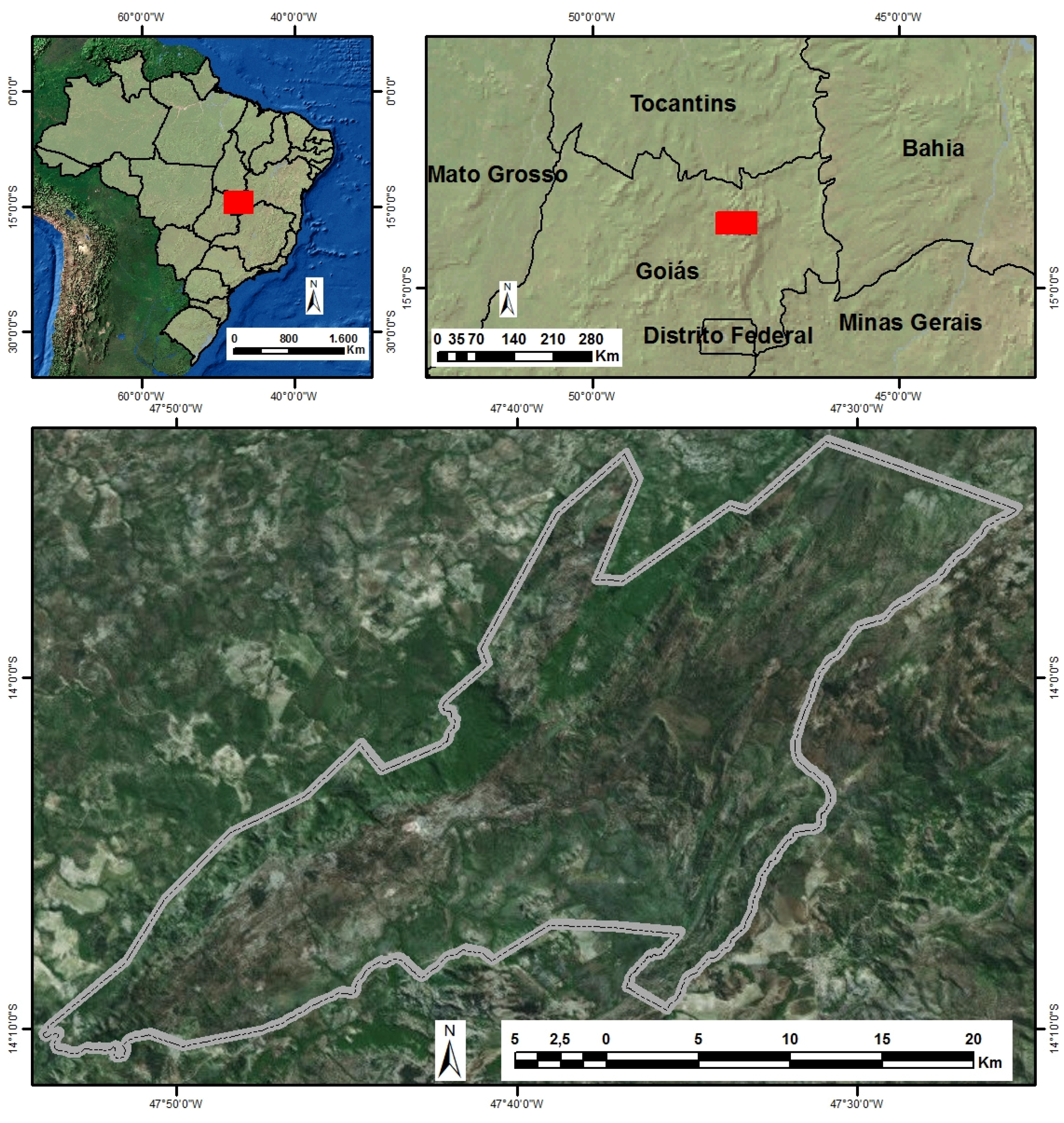
The study area is the Chapada dos Veadeiros National Park (CVNP) (655 km²) located in Central Brazil. This park was included in the World Heritage List by UNESCO in order to preserve the flora, fauna and key habitats that characterize the Brazilian Savanna (Figure 1).

Figure 1. Chapada dos Veadeiros National Park location.

Figure 1. Chapada dos Veadeiros National Park location.

The CVNP has a stunning natural beauty, especially due to the waterfalls, vertical escarpments, canyons and rivers [45]. The CVNP corresponds to the uppermost parts of the Brazilian Central Plateau (BCP), having its peak in the region of Pouso Alto with an altitude of 1676 meters. The geomorphology has a strong lithological and structural control. The CVPN is in the northern sector of the Brasília fold-and-thrust-belt, which is a major tectonic unit of the Tocantins Province in Central Brazil, resulting from the Neoproterozoic collision episode between São Francisco and Congo cratons [46]. In the CVNP, the predominant rocks are quartzites and meta-siltstones that due to its high resistance to physical and chemical weathering generate shallow soils with low fertility [45].

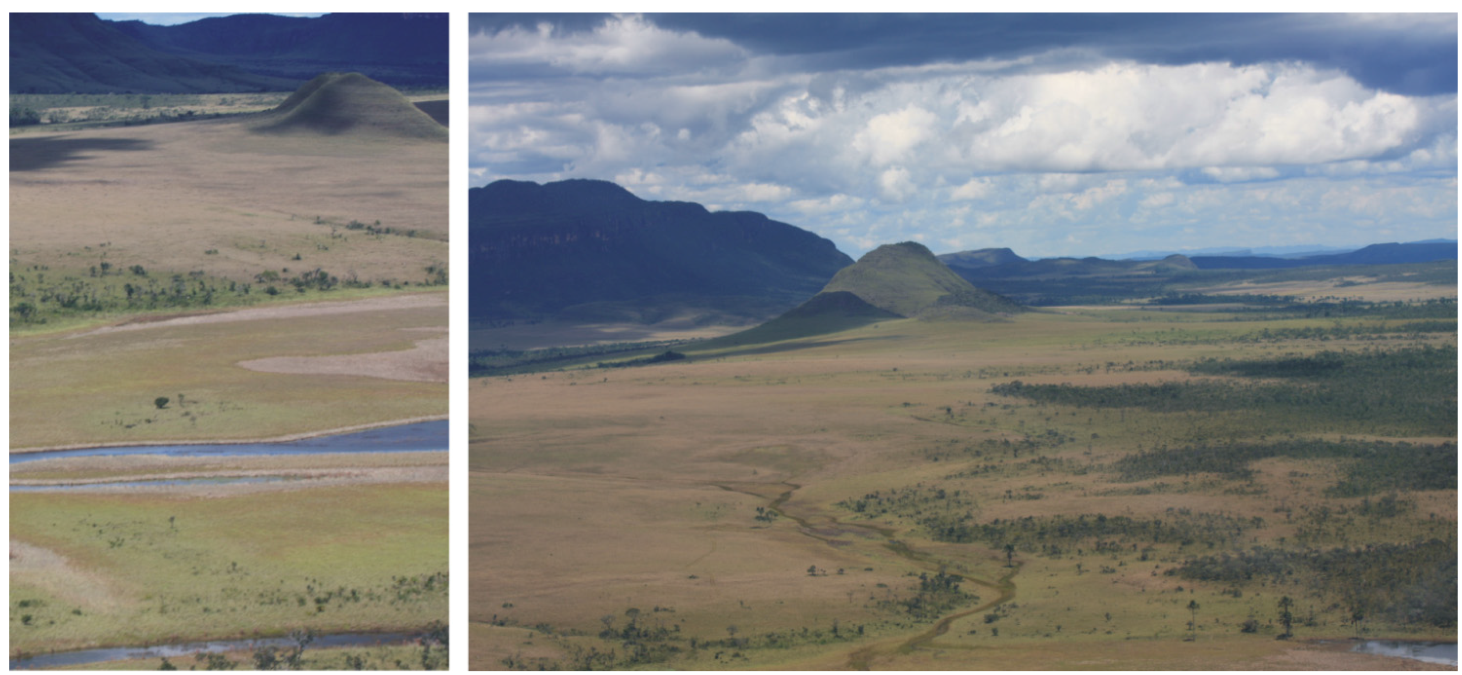
The CVNP is contained in the Cerrado Biome, the most diverse tropical savanna and one of the world’s biodiversity hotspots [47,48]. Furthermore, in this biome, the number of native vascular plants is higher than most regions of the world, containing 6429 records, however, the total estimate may be as high as 10,500 [49,50]. The savanna physiognomies express a ratio between the continuous herbaceous and discontinuous layer of shrubs and trees [51]. 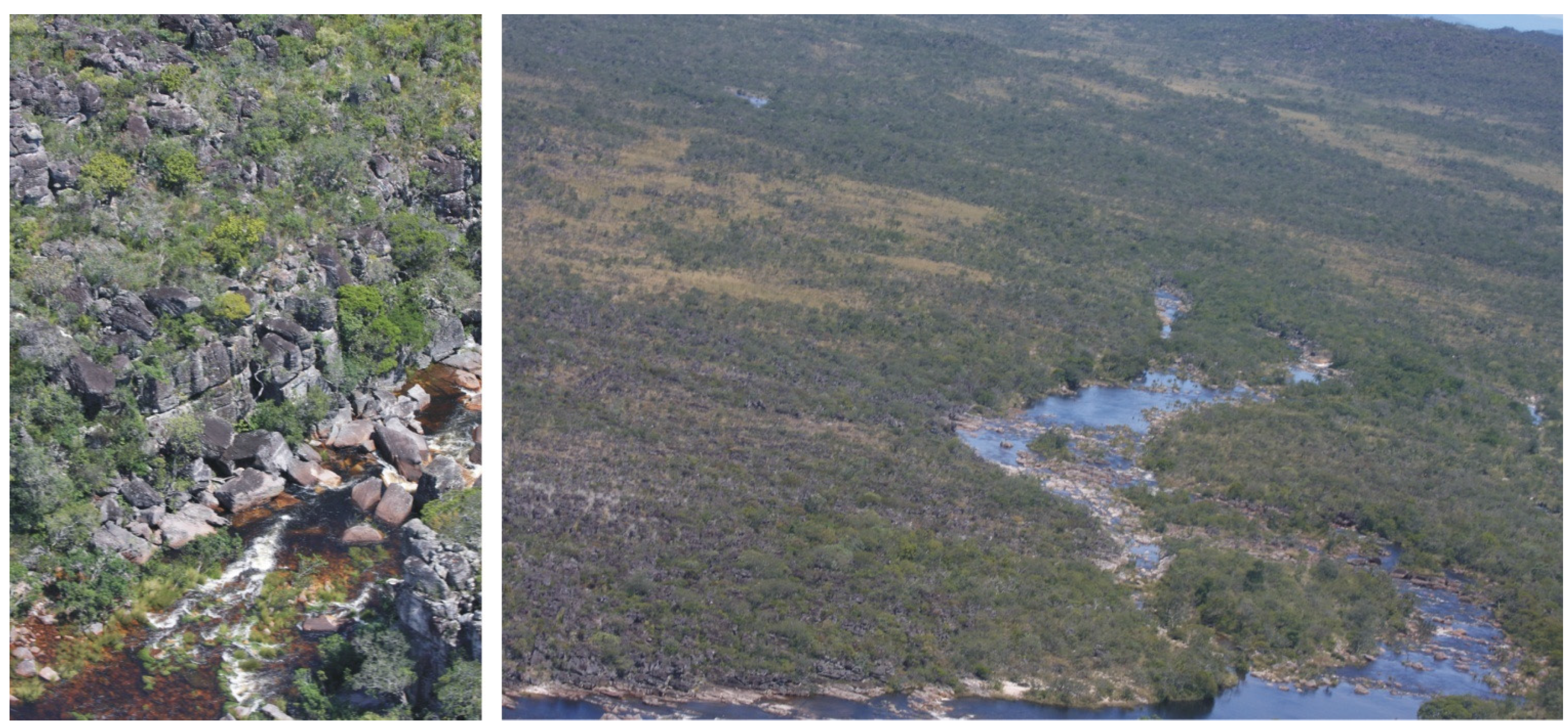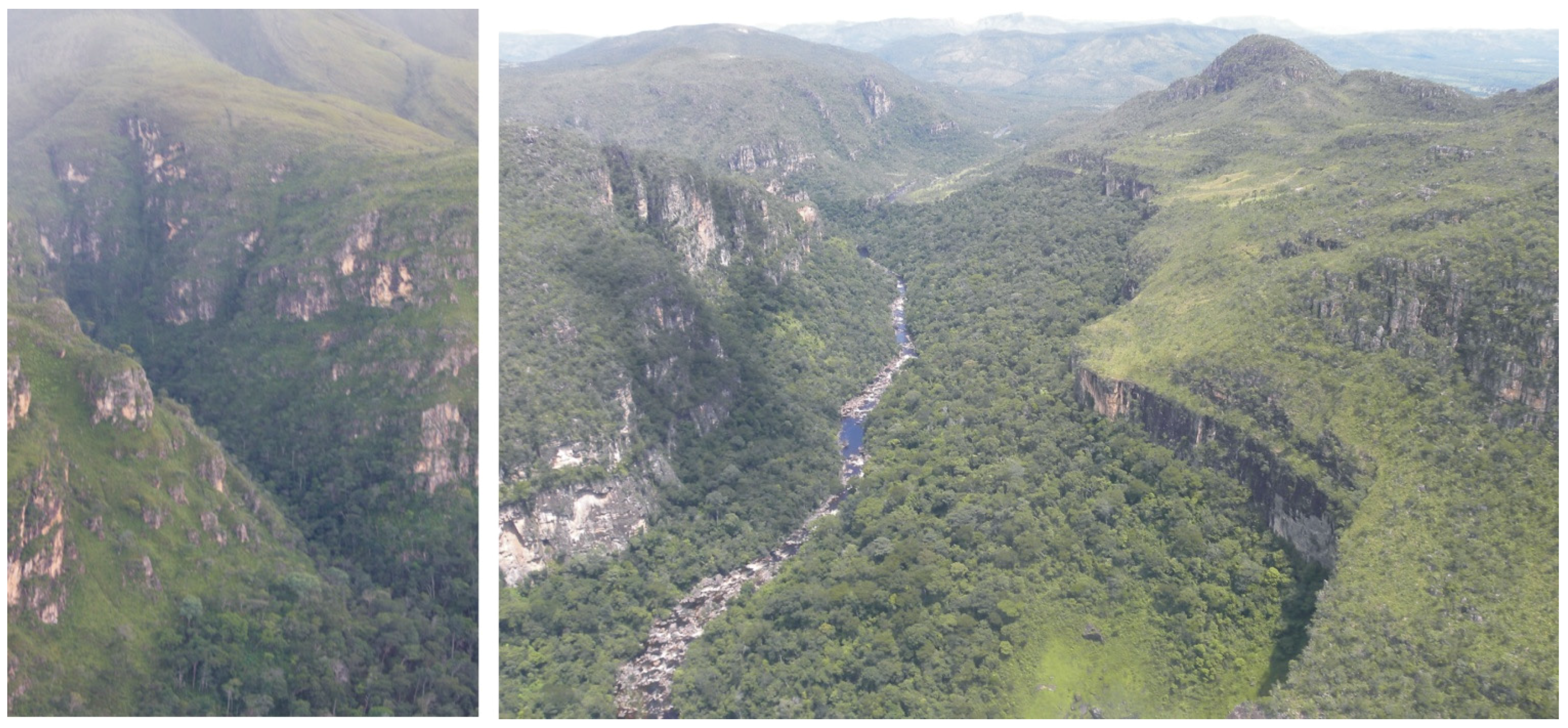In the CVNP, the most representative vegetation in the range of densities of the woody plant layer are: (a) Grassland (grasses, herbs and some very low shrubs or trees) (Figure 2); (b) Savanna on rocky outcrops (Figure 3); (c) Savanna (tree–grass mixtures); (d) Closed Savanna Woodland (densely covered by trees) (Figure 4) [52].

The region has a tropical precipitation regime characterized by well-defined wet (October to April) and dry (May to September) seasons. This ecosystem shows hydrological constraints in the dry season, which propitiates a fire-event concentration in just a few months of the year. During the dry season, the grassy herbaceous biomass becomes especially dry and very flammable [53]. Therefore, the Cerrado species are adapted to a natural fire regime. Furthermore, the CVNP and its surrounding areas are very susceptible to fire events caused by human activities [53,54]. In the areas with human intervention, the burning usually happens at intervals of three years in order to induce the vegetation regrowth and the increase food availability for the cattle.

Figure 2. Panoramic photographs of the open grasslands in the Chapada dos Veadeiros National Park.

Figure 2. Panoramic photographs of the open grasslands in the Chapada dos Veadeiros National Park.

Figure 3. Panoramic photographs of the savanna on rocky outcrops in the Chapada dos Veadeiros National Park.

Figure 3. Panoramic photographs of the savanna on rocky outcrops in the Chapada dos Veadeiros National Park.

Figure 4. Panoramic photographs of the Closed Savanna Woodland in the Chapada dos Veadeiros National Park.

Figure 4. Panoramic photographs of the Closed Savanna Woodland in the Chapada dos Veadeiros National Park.

3. Materials and Methods

3.1. MODIS/Terra Time-Series Data

In this study, we used the MODIS/Terra Surface Reflectance 8-Day composite data, which includes seven spectral bands at 500-meter resolution (MOD09A1) and two bands at 250-meter resolution (MOD09Q1). The MODIS/Terra data are freely distributed through the Earth Observing System Data Gateway. MOD09 product yields the best surface spectral-reflectance data for each 8-day period with the least effect of atmospheric water vapor. The images already have atmospheric corrections for gases, thin cirrus clouds and aerosols [55]. The MODIS data is increasingly used to monitor burned areas and active fire over large geographic areas (e.g., [56,57,58,59,60,61,62,63]). The study area is contained in just one MODIS scene (tile h13v10). We specifically used the band 2 (0.841–0.876 μm) at 250-meter and the band 7 (2.105–2.155 μm) at 500-meter. The band 7 was resized from 500-meter to 250-meter resolution using the nearest neighborhood resampling. The NBR index is calculate using the bands 2 and 7 as follows: NBR = (Band 2 − Band 7)/(Band 2 + Band 7). In this research, we used 552 images for the period 2001–2012 over the same area. A representation of the NBR image collection can be obtained by building the cube of MODIS temporal series [64,65]. The cube is formed by images of the temporal series with its three dimensions: x, y and z (NBR temporal curve) acquired in the same geographical area at different times.

3.2. Noise Elimination

Temporal quality in orbital images is difficult to be maintained due to atmosphere interferences (aerosols, clouds and shadows effects), which cause serious problems and hinders the identification and quantification of targets. Therefore, different methods have already been proposed to reconstruct remote-sensing time series (e.g., [66,67,68,69]). In this work, we used Savitzky and Golay (S-G)’s method to remove noise contamination in the images, which is based on local polynomial fits. The S-G filter was originally developed for the smoothing of noisy data from chemical spectrum analyzers [70]. The great advantage of S-G filter is to combine the effective noise removal and the waveform-peak preservation considering the following attributes: height, shape and asymmetry. This peak-preservation property is very attractive for the phenological analysis from remotely sensed data. Thus, Chen et al. [71] propose a method based on the S-G filter to smooth the effects of cloud contamination and atmospheric variability on the NDVI time-series. Based upon this study, different researches show the successful application of the S-G filter in the MODIS vegetation indices, by minimizing overall noise and preserving higher vegetation-index values (e.g., [69,71,72]). Geng et al. [67] compare eight techniques for smoothing multi-temporal NDVI data, considering different vegetation types and sensors, and conclude that the S-G filter achieve best results in most situations.

In the fire analysis using time series, the preservation and maintenance of negative peaks of NBR and NDVI values become important for the detection and characterization of the burned areas. The S-G method is suitable for this proposal, since other smoothing methods cannot capture a sudden change of the temporal values, for example Fourier series or least squares fitting to sinusoidal functions [73,74,75]. The choice of the window width in the S-G filter is essential to provide smoothing without loss of resolution. The wide windows can eliminate significant changes in temporal series, while a narrow window can hold more noise [71]. In this work, we developed a program for time series analysis containing the S-G filter. The S-G method is used both for smoothing the time series as to remove the noise contamination. The method for detecting outliers effects the subtraction between the S-G curve and the original data. Therefore, the point is marked as an outlier if the absolute value of the subtraction exceeds a distance threshold set by the user (either positively or negatively). 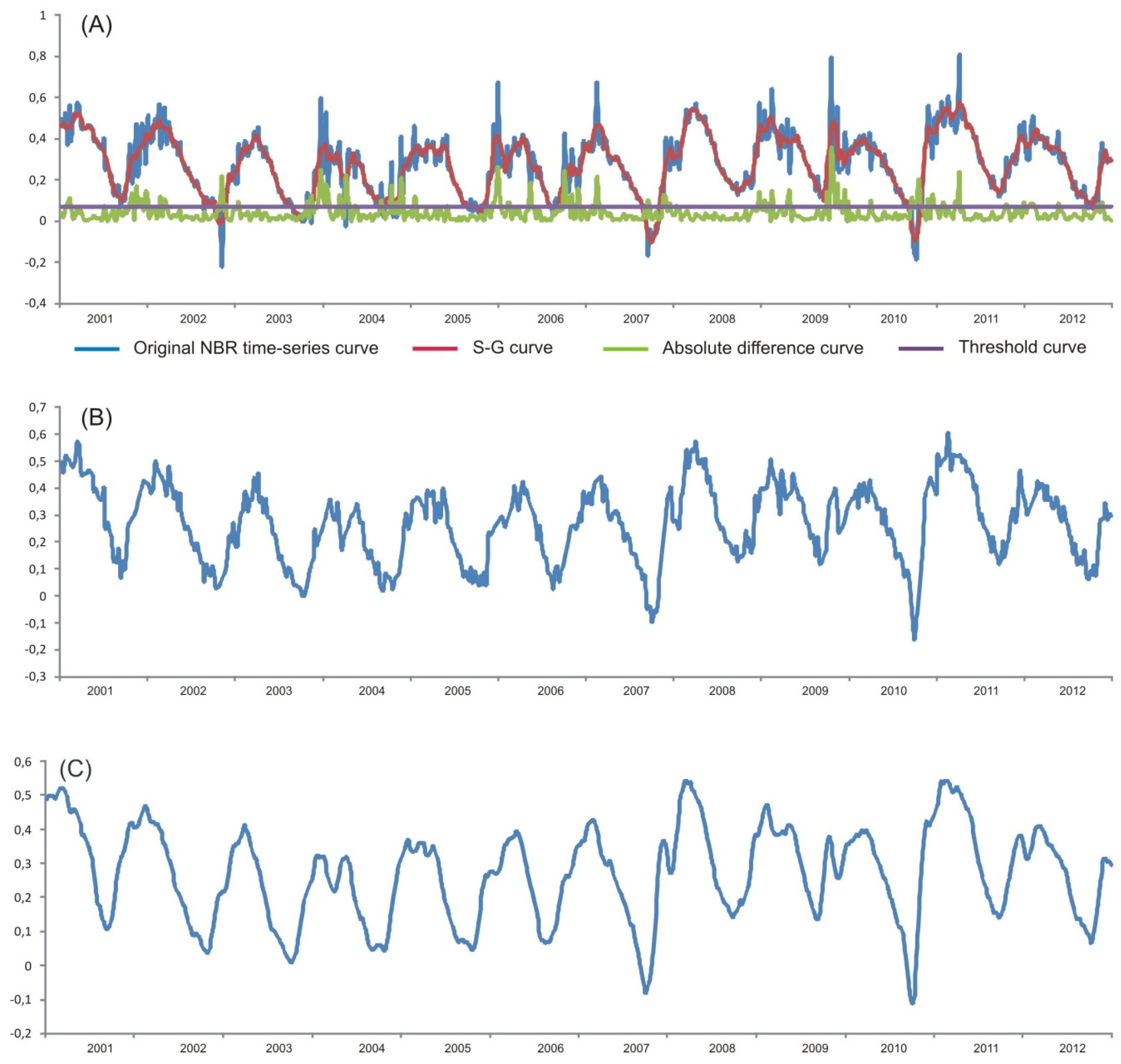The distance-based outliers are replaced by the value obtained by linear interpolation between the points before and after the outliers (Figure 5). In this procedure, only the outliers are modified and the remaining points are from the original curve. The software allows the user to test and visualize the resulting temporal curve considering different window sizes and distance thresholds for a given pixel of your choice before processing the whole image. In the pre-processing of the MODIS NBR time series, the two procedures were performed in sequence, first the removal of outliers and then smoothing the temporal curve. The window size of the S-G filter in both procedures was nine. The distance threshold of 0.07 NBR was used in the outlier detection.

Figure 5. Procedures for reconstruction of a NBR-MODIS time series using two-step filtering approach through the S-G method. (A) Outlier detection using the absolute value of the difference between the original data and the S-G curve (distance threshold of 0.07). (B) Time-series curve with the outliers replaced by a linearly interpolated value. (C) Time-series curve after the second filtering by S-G method (window size of 9).

Figure 5. Procedures for reconstruction of a NBR-MODIS time series using two-step filtering approach through the S-G method. (A) Outlier detection using the absolute value of the difference between the original data and the S-G curve (distance threshold of 0.07). (B) Time-series curve with the outliers replaced by a linearly interpolated value. (C) Time-series curve after the second filtering by S-G method (window size of 9).

3.3. Standardized Time-Series

The Cerrado biome has a high natural variability with a continuous range of percent tree cover, resulting in different phenological signatures. One way to harmonize the different temporal curves is using the z-score standardization [76,77], defined as:

$$z=\frac{x-\mu }{\sigma }$$

(1)

where “μ” and “σ” are the mean and standard deviation of the temporal series, respectively. Initially, the algorithm generates mean and standard deviation for each temporal curve. A new set of images is generated, containing transformed temporal curves of “z” values, i.e., mean equal to zero and variance of one. The “z” value is positive when raw score is above of temporal mean and negative when below.

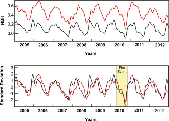
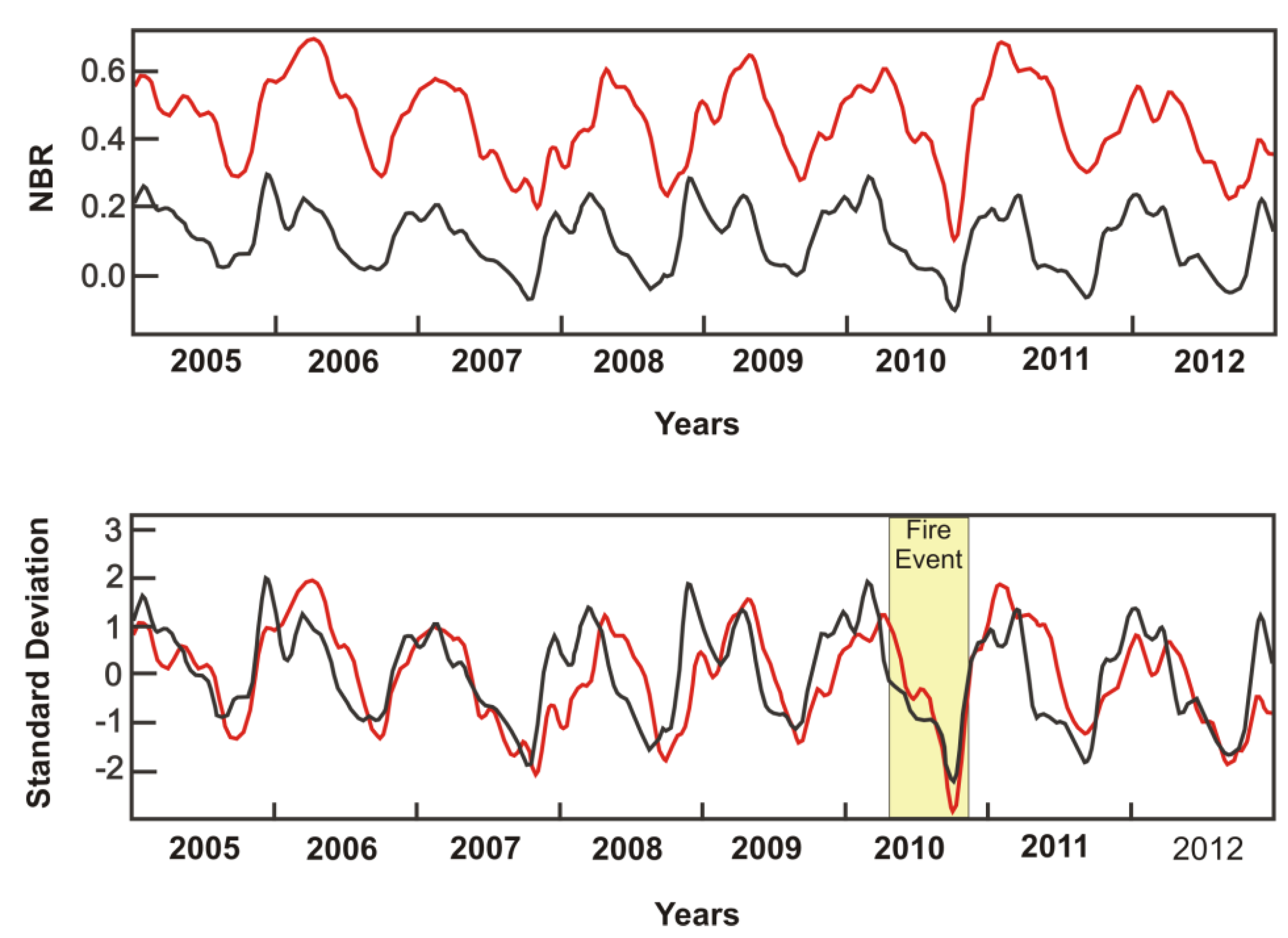
Figure 6 shows the standardization effect at temporal curves considering two Cerrado-vegetation types. Burned areas cause a fall in the NBR values, but present distinctions for each environment. The red curve shows higher values than the black curve even after burning. A simple threshold would not be able to differentiate simultaneously the burned areas in both types of vegetation. Temporal curves after the standardization procedure acquire a similar behavior, where the burned areas have compatible values and able to be separated by a single cutoff.

The fire is an isolated event characterized by low NBR values in the time series. The burned areas occur at confidence interval described by a threshold value from the mean time series. A constant expressed in standard deviation determines lower limit. This measure allows the comparison of different vegetation simultaneously. The best threshold can be determined based on the comparison with known burned areas.

Figure 6. NBR-MODIS time series of savanna (black curve) and Closed Savanna Woodland (red curve) before and after the standardization. The standardized temporal curves homogenize and highlight the fire event, which reached different types of vegetation.

Figure 6. NBR-MODIS time series of savanna (black curve) and Closed Savanna Woodland (red curve) before and after the standardization. The standardized temporal curves homogenize and highlight the fire event, which reached different types of vegetation.

3.4. Interannual Phenological Deviation

A reference curve of interannual phenological behavior for each pixel creates a baseline from which the time series are subtracted, minimizing the seasonal component and emphasizing the fire changes. The dNBR_MODIS method performs a seasonal difference, in which the baseline is the previous year. Thus, the procedure is carried out by subtracting the value of each observation exactly one year earlier. However, this approach is susceptible to high signal-to-noise ratio [41]. If the previous year contains fire events, the seasonal-difference values are very high, though it does not represent a change event to the date concerned. Furthermore, the result of seasonal difference has one year less than the original time series.

In this context, seasonal phenological curves from measures of central tendency may have greater advantages as baseline than the use of the previous year. The central-tendency curves enable to distinguish long-term trends of random fluctuations. These measures emphasize the vegetation behavior in order to minimize the fire effects. The adoption of this approach can reduce the signal-to-noise ratio, and the output data has the same size as the input time series. The measures of central tendency used in this work were mean, median and trimmed mean.

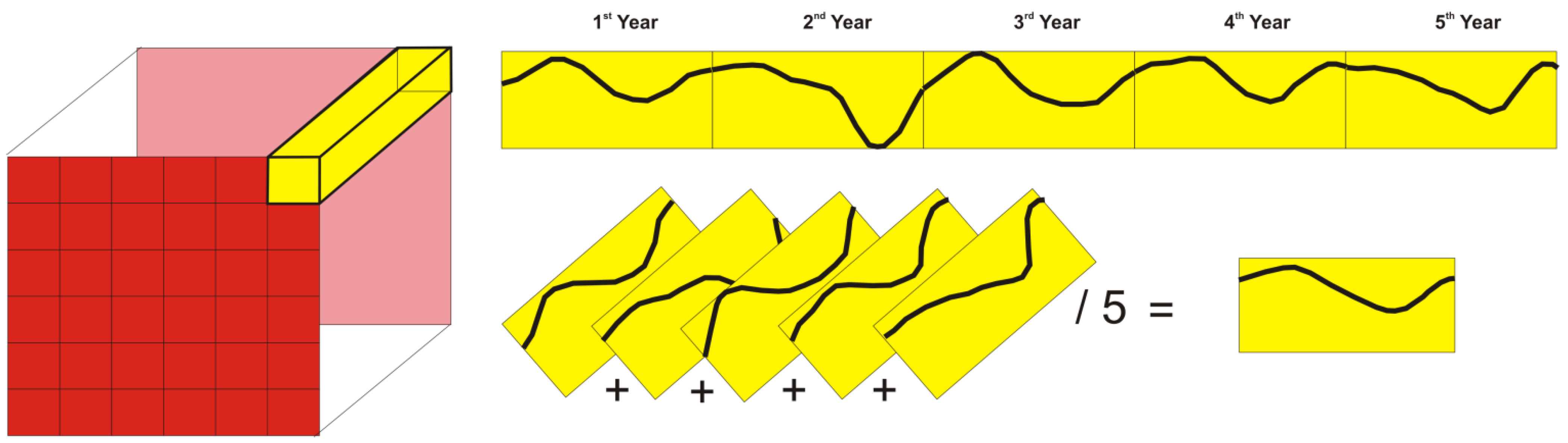
The mean curve calculation is the sum of the NBR values for a same eight-day period in the different years divided per year range (Figure 7). This measure is appropriate when the fire recurrence is very low. The fire recurrence provokes a decrease in the NBR mean values, impairing an adequate representation of the annual cycle of vegetation.

Figure 7. Procedure for calculating interannual mean curve, considering a pixel and five-year period.

Figure 7. Procedure for calculating interannual mean curve, considering a pixel and five-year period.

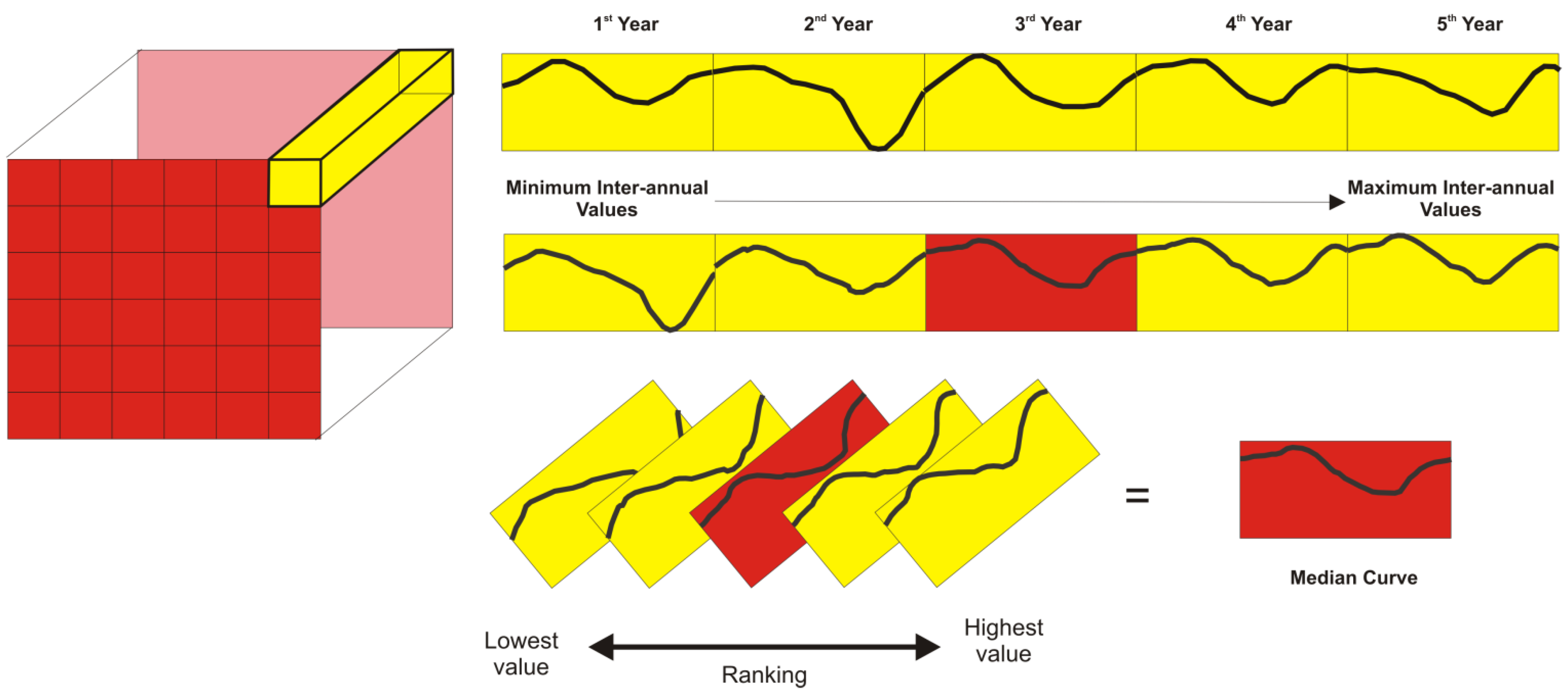
The median is known for being particularly effective in removing changes of short duration. The median is a particular case of the ith order statistic (or rank statistic) of a finite set of real numbers. Arranging all the observations from lowest to highest value, the median value is the middle one. Considering an order statistic of N real numbers (x(i)...,x(N)), where N is number of years, the minimum is then x(1), the maximum x(N), and the median X((N + 1)/2). The calculation of the interannual median is performed separately for each eight-day period in the several studied years. In this way, the method initially gathers the first 8-day period of every year (e.g., 1st 8-day: 2001; 1st 8-day: 2002, etc.) and calculates the median, which is contained in the first band of the result image. Then, the same procedure is performed for the second 8-day period (e.g., 2nd 8-day: 2001; 2nd 8-day: 2002, etc.) composing the second band, and so forth. Therefore, the z-profile from median interannual image has the same dimension as one particular year (Figure 8). The implementation of a median requires a very simple digital nonlinear operation. In this case, if the fire events are present in a few years over a time series, the median can eliminate their influence.

Figure 8. Procedure for calculating the interannual median curve, considering one pixel and five years.

Figure 8. Procedure for calculating the interannual median curve, considering one pixel and five years.

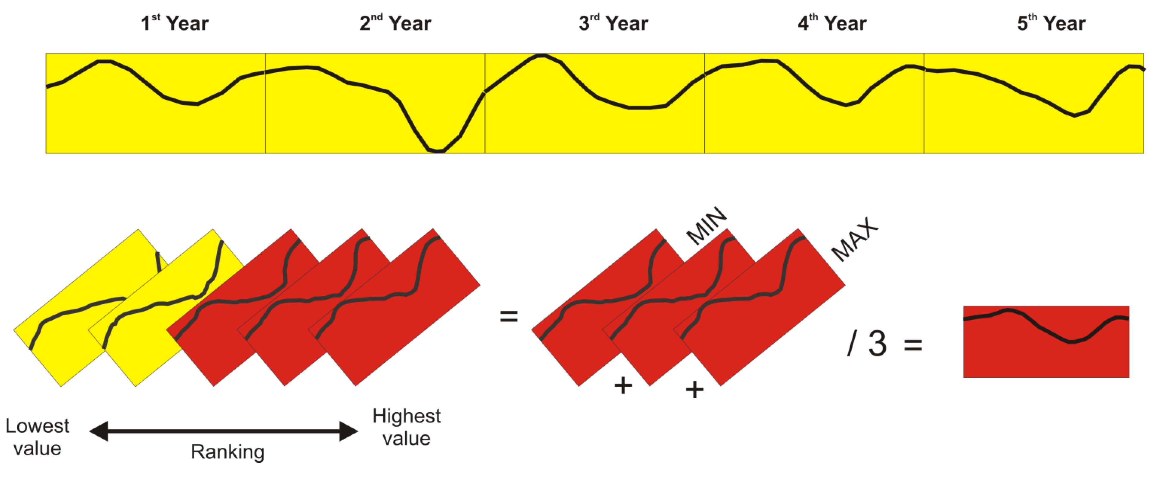
Most environments, the annual median curve eliminates the fire events. However, the median can be mistaken if the fire recurrence surpassing half years in analysis. For this case, we propose the trimmed mean as an adaptation of the alpha-trimmed mean. The alpha-trimmed mean is a measure between median and mean values [78]. This method also made a rank statistic (x(i)...,x(N)), where N is number of years. The user indicates an alpha value, percentage of the trimmed sample, which is used to eliminate samples that are more distant from the median. Alpha values vary between 0 and 0.5. Thus, the method performs the mean calculation considering only the inner sample values (the ones close to the median). The result is equal to median when alpha is close to 0.5 and mean when alpha is close to 0. The proposed algorithm in this paper allows the user to choose the maximum and minimum position in an ascending order of NBR values for calculating the mean (Figure 9). This procedure allows choosing higher NBR values to ensure exclusion of the noisy data. In this research, all possible alpha values were considered. Each point on the interannual curve has a set with N = 12 (corresponding to the study period), where the data is ordered followed by elimination of extreme values. The inner sample quantity may be equal to 10, 8, 6 and 4 (12 is equivalent to the mean, while 2 is equivalent to median), i.e., with alpha values equal to 0.1, 0.2, 0.3, and 0.4, respectively.

The interannual phenological deviation is the difference between the value of an observation and the average interannual for the same pixel and calendar day. Deviation-image analysis enables highlighting the changes in the time series. Burned areas show a marked drop of deviation values in the temporal curve, favoring its delimitation by a threshold value.

Besides, we compute the interannual standard deviation among the seasonal NBR curves (result with the number of samples throughout the year) and the intra-annual standard deviation (result with the number of analyzed years). The interannual standard deviation demonstrates the days of the year with the highest rates over the time series. While the intra-annual standard deviation show the years with greater variation.

Figure 9. Procedure for calculating the interannual trimmed mean curve, considering one pixel and five years.

Figure 9. Procedure for calculating the interannual trimmed mean curve, considering one pixel and five years.

3.5. Optimal Threshold-Value Definition

A key procedure in the burned area detection is the appropriate selection of an optimal threshold value between burned area and unburned area. The threshold values are often determined empirically and depend on the image and the analyst’s knowledge [79]. In this paper, we used a specific method for definition of the optimal threshold value [79,80,81], which compare the classified maps from different threshold values with a reference map elaborated from accurate image classification, usually with higher spatial resolution. Confusion matrices were calculated between the reference maps and a set of classified maps, considering a continuous sequence of threshold values. The optimal threshold value is the point with the maximum Kappa or Overall coefficient, i.e., accuracy indices extensively used to assess accuracy [82]. The overall accuracy is the sum of the number of pixels classified correctly divided by the total number of pixels. The Kappa coefficient (K) is an accuracy measure of the classification described by the following equation:

$$K=\frac{m{\displaystyle \sum _{i=1}^r{s}_{ii}-{\displaystyle \sum _{i=1}^r{s}_{i+}{s}_{+i}}}}{m^2-{\displaystyle \sum _{i=1}^r{s}_{i+}{s}_{+i}}}$$

(2)

where “r” is the number of rows in the error matrix, “s_ii” is the number of observation on row “i” and column “i”, “s_i+” and “s_+i” are thus the marginal totals on row “i” and column “i”, respectively, and “m” is the total number of observations.

In addition, the sensitivity (true positive rate, expressed as a percentage) and specificity (true negative rate, expressed as a percentage) curves were calculated to evaluate the best threshold. The increased specificity implies a decreased sensitivity and back again. Each sensitivity/specificity pair corresponds to a particular decision threshold. Normally, the intersection of the two curves represents the threshold point near the highest Overall Accuracy and Kappa coefficient. Therefore, the closer the curve intersection is to the upper (100%), the higher the accuracy of the test.

Furthermore, the algorithm developed for the detection of the optimum threshold value allows as input data more than one image pair containing different dates. The method calculates a unique confusion matrix from several image pairs (reference and normalized images). The same effect can be obtained from the sum of the confusion matrices of independent image pairs. The accuracy indices are calculated from the resulting confusion matrix.

In this purpose, we elaborated two reference maps of the burned areas from the digital image processing and visual interpretation of Landsat TM (30-meter resolution) in order to determine the optimal threshold value. The image dates were 25 October 2007 (Julian day 274) and 29 September 2010 (Julian day 266) because of the extensive burned area and no cloud cover. The first image contains a burned area of 660 km² corresponding to 39.6% of the studied image while the second image contains a burned area of 1030 km² that matches 61.7%.

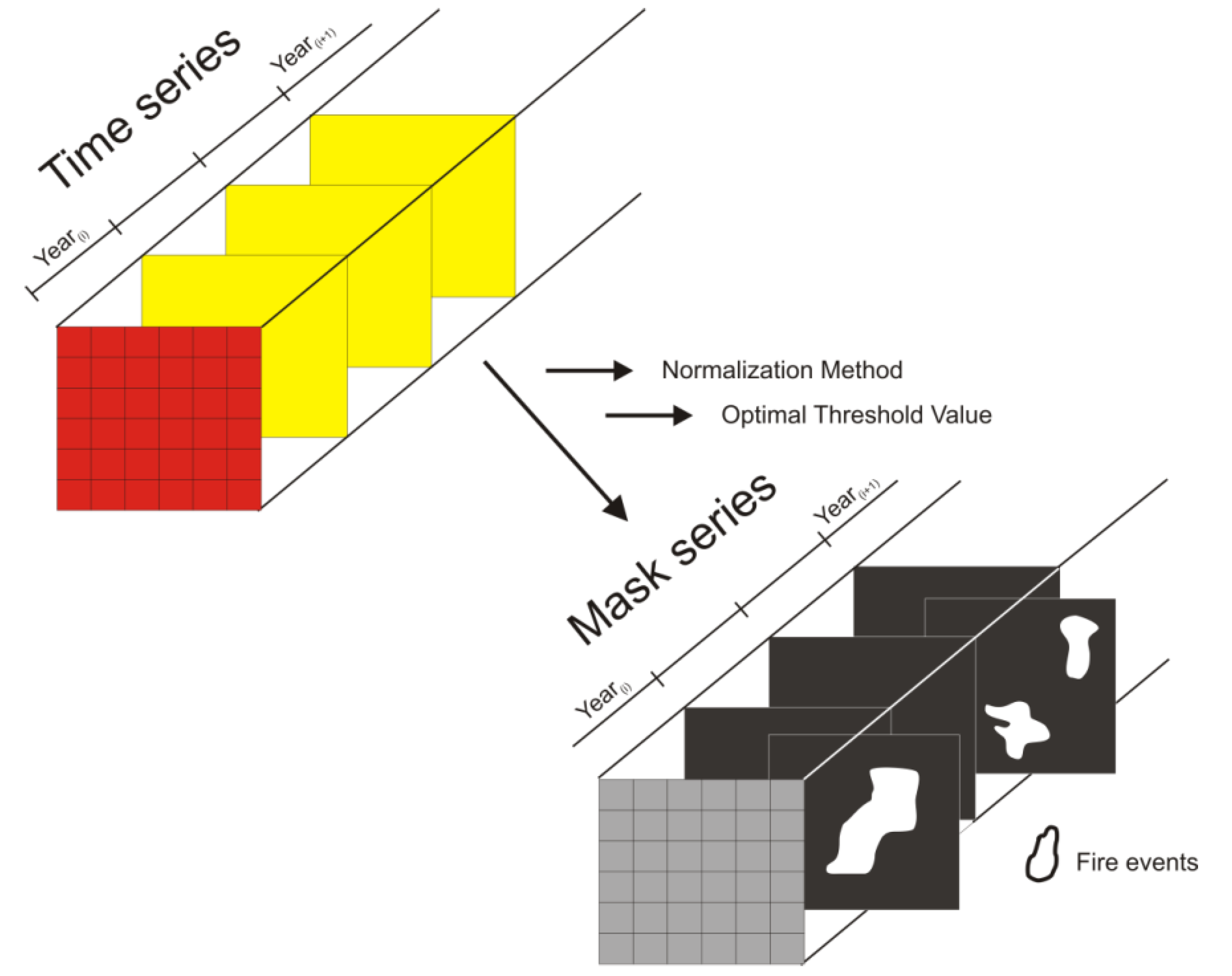
The optimal threshold value from accuracy analysis was applied to all time series (12 years) generating a mask series of burned areas (Figure 10). An inverse validation with independent data was used to quantify the goodness/advantages of the proposed methods. An additional reference map of burned areas from the Landsat TM image (22 September 2004) was compared with the burned-area masks of the respective day extracted from the MODIS image and the proposed methods.

Figure 10. Mask series of the fire events detected in the time series.

Figure 10. Mask series of the fire events detected in the time series.

4. Results

4.1. Results of the Standardized Time-Series Method

4.1.1. Standardized Images

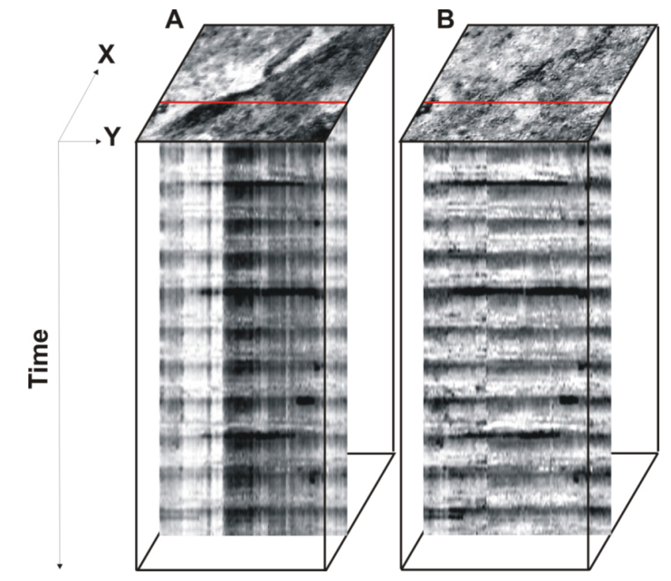
The standardization of the time series for each pixel reduces the differences between vegetation types and highlights the episodic fire events. Z-score model provides a measure in relation to its mean expressed as a percentage of the standard deviation. Figure 11 compares the original and standardized images and its respective horizontal slice images. Horizontal slice image combines spatial and temporal profile of a multi-band image, where all the bands of a single line make up a grayscale image in which the number of bands is equal to the number of lines. The slice image from the NBR image shows a strong differentiation between areas with forest formation (highlighted in light tones) and the savanna and grassland formations (with darker tones) (Figure 11A). In contrast, the slice image of standardized data has seasonal variations as the main tonal variation (Figure 11B).

Figure 11. Original (A) and standardized time-series (B) images and its respective horizontal slice images.

Figure 11. Original (A) and standardized time-series (B) images and its respective horizontal slice images.

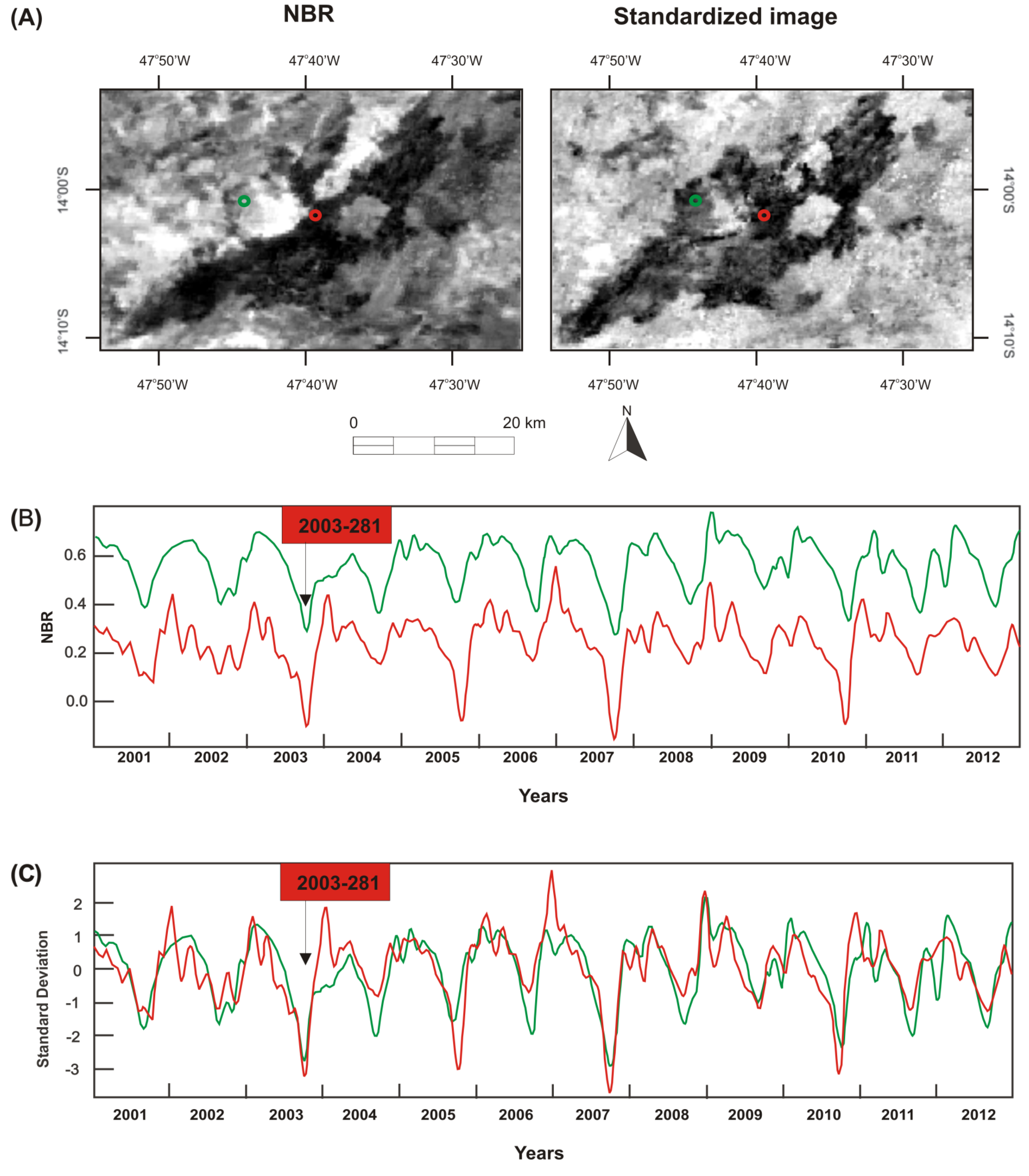
Figure 12 shows the use of the standardized times series in the enhancement of the burned areas. The comparison between the NBR and standardized time-series images evidences that the method provides a better detailing of burned areas. In both images, the burned areas are demarcated in a dark tone. In the NBR image, burned areas on close woodland savanna (red point in the Figure 13) exhibit intermediate grayscale, which makes these features hard to see. In these places, the NBR values show a decrease but not enough to become noticeable in the image. In contrast, the standardized time-series images can detect the burned areas with continuous extension through different vegetation types. Therefore, the automatic mapping of burned area from long-term time series is facilitated using standardized image.

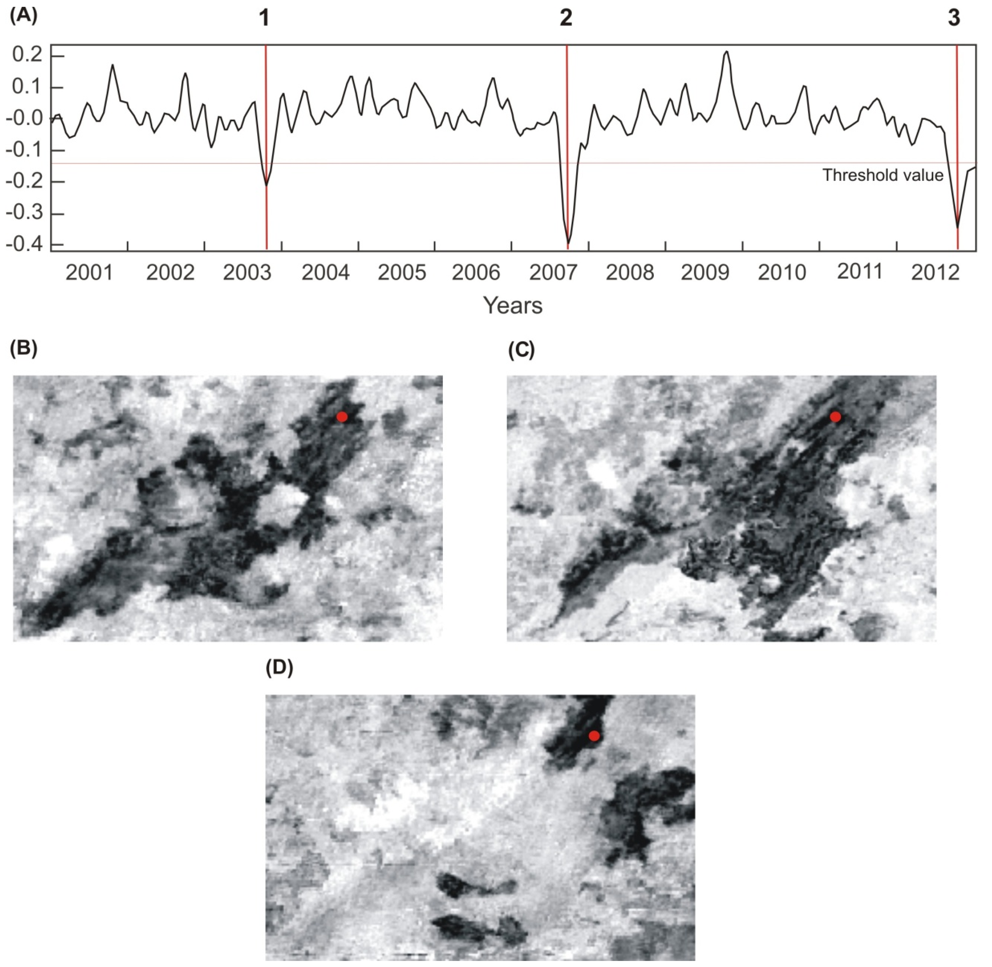
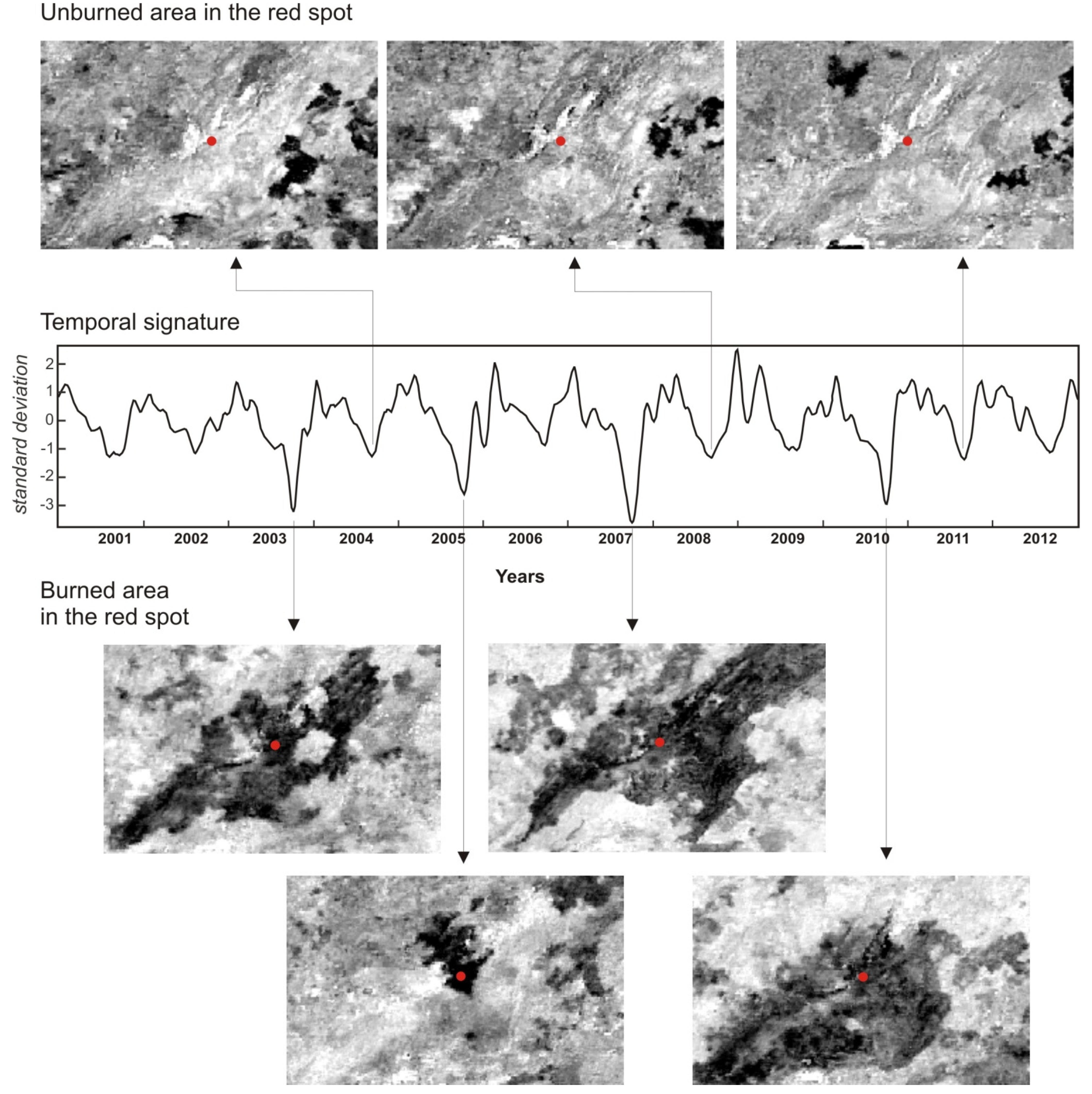
In this procedure, the burned areas are expressed with negative values of standard deviation. Figure 12 shows the temporal curve of a red point on the image for a period of 12 years and the different behavior of burned and unburned events. All burned events are easily detectable by having standard deviation values much lower than other periods of the temporal curve.

Figure 12. Comparison between the NBR and NBR standardized data: (A) NBR-MODIS composite image (Julian day 281–2003) and its respective standardized image, (B) NBR temporal curves for the savanna (red point) and Closed Savanna Woodland (green point), and (C) NBR standardized temporal curves for the same points.

Figure 12. Comparison between the NBR and NBR standardized data: (A) NBR-MODIS composite image (Julian day 281–2003) and its respective standardized image, (B) NBR temporal curves for the savanna (red point) and Closed Savanna Woodland (green point), and (C) NBR standardized temporal curves for the same points.

Figure 13. Temporal curve for the 12-year period emphasizing some standardized images. The red dot in the images demarcates the location of the time curve. The images in the upper part correspond to the unburned period. While the images at the bottom point out burned events, during the analyzed period.

Figure 13. Temporal curve for the 12-year period emphasizing some standardized images. The red dot in the images demarcates the location of the time curve. The images in the upper part correspond to the unburned period. While the images at the bottom point out burned events, during the analyzed period.

4.1.2. Threshold Value for Burned-Area Detection Using Standardized Time-Series Images

The MODIS-NBR standardized time-series images were classified using an optimum threshold value obtained from the best fit with the Landsat TM classification. Therefore, the optimum threshold value is determined from accuracy assessment curves, which considers different threshold values on the x-axis plotted against its respective accuracy indices on the y-value (i.e., Kappa coefficient, Overall Accuracy, Sensitivity and Specificity). The confusion matrices of the two reference images (25 October 2007 and 29 September 2010) were integrated to generate a single set of curves for the optimum-threshold selection. 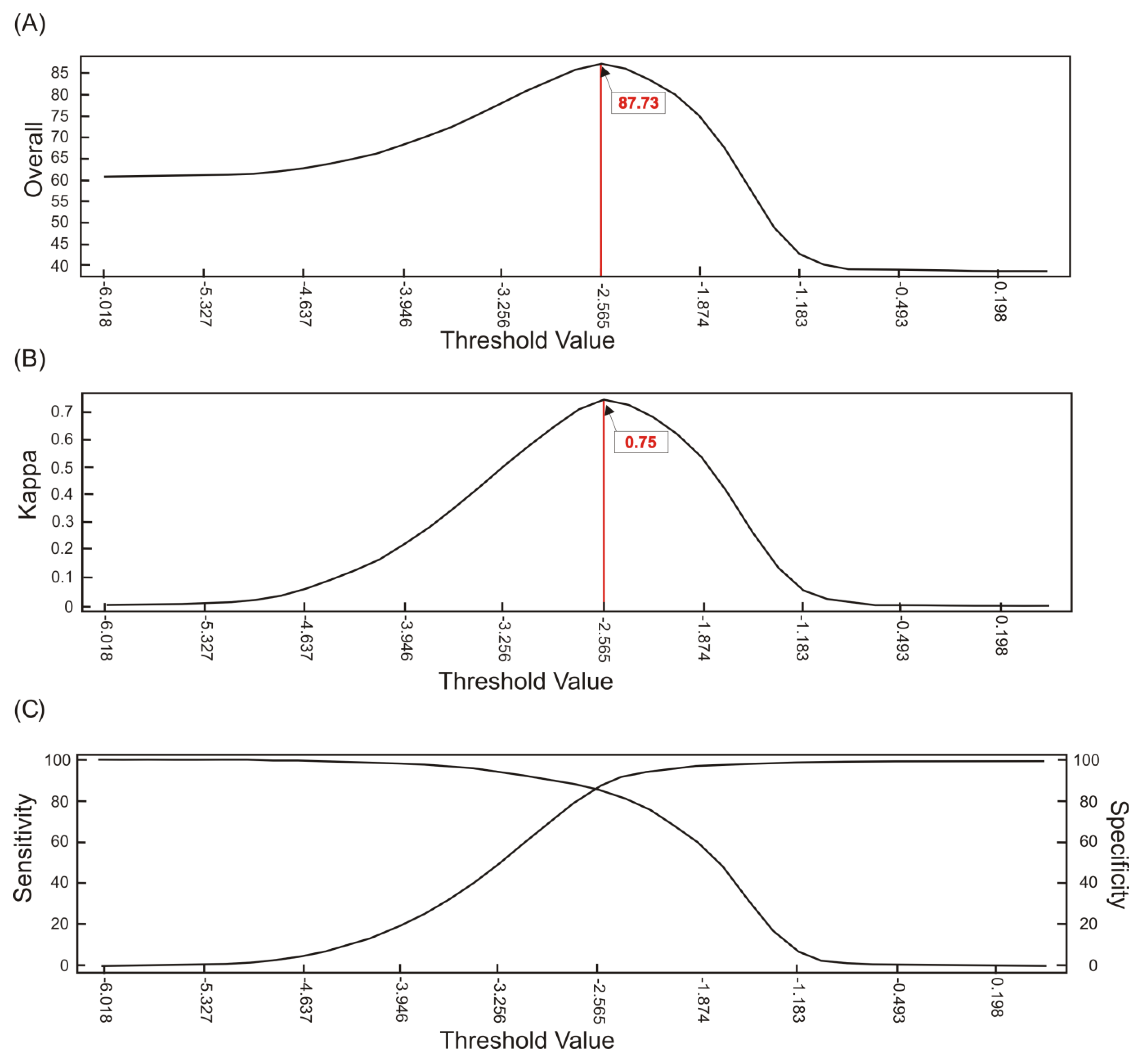The best-fit threshold was −2.565 standard deviations, containing 87.73% of the Overall Accuracy and 0.75 of the Kappa coefficient (Figure 14). The intersection between Sensitivity-Specificity curves had a consistent position with the Kappa coefficient and the Overall Accuracy. The threshold value set by Kappa coefficient was applied to the whole time series, generating mask series relating to fire events for each image of the time series.

Figure 14. Identification of the optimal threshold values for burned-area detection from the standardized temporal series images. The accuracy assessment curves refer to the following indices: (A) Overall accuracy, (B) Kappa coefficient, and (C) Sensitivity-Specificity pair.

Figure 14. Identification of the optimal threshold values for burned-area detection from the standardized temporal series images. The accuracy assessment curves refer to the following indices: (A) Overall accuracy, (B) Kappa coefficient, and (C) Sensitivity-Specificity pair.

4.2. Results Interannual Phenological Deviation

4.2.1. Results of the Average Interannual Phenology

The NBR average annual corresponding to a 12-year period (2001–2012) evidenced the phenological behavior at each pixel of the image. The measures of central tendency (mean, median and trimmed mean) lead to a noise minimization and provide an appropriated baseline to be compared over time for each pixel. The key issue is to establish for each pixel a phenological curve to be employed in the burned-area detection, instead of the previous year used in the seasonal differencing.

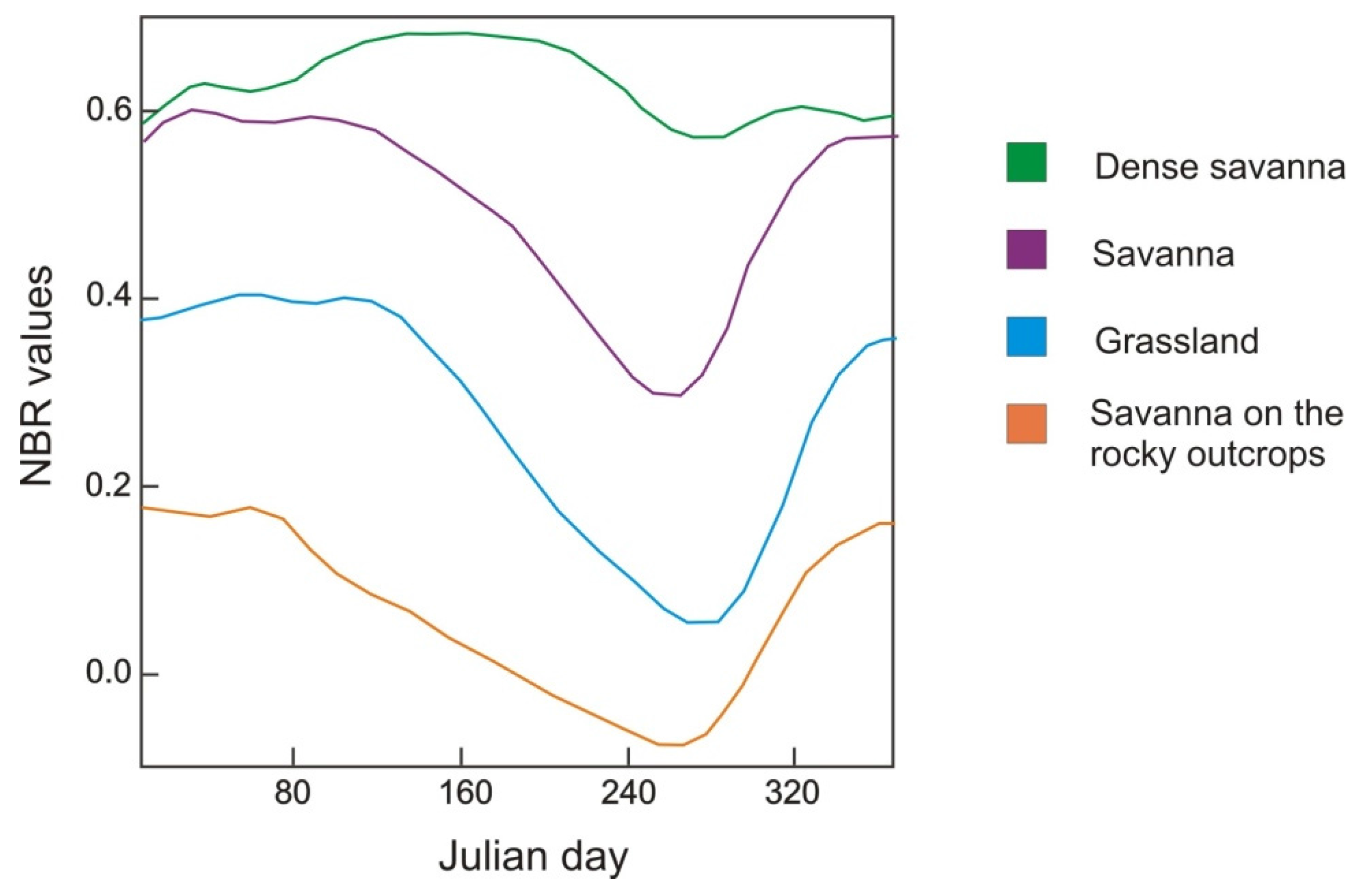
Figure 15 shows the mean phenological signatures for major vegetation types in the CVNP. Savanna on rocky outcrops has the lowest NBR values, probably due to interference and mixed spectral with the areas of outcropping rocks. NBR values increase gradually with the increment of arboreal covering open grassland to dense Cerrado. The phenological curve of the dense Cerrado presents the highest NBR values and a delay of leaf senescence compared to other vegetation. Carvalho et al. [83] observe that the dense Cerrado at the beginning of the dry season (June) has the following characteristics: chlorophyll a and b concentrations were higher, chlorophyll a/b ratio was lower, and total chlorophyll/carotenoids ratio is significantly greater to the higher chlorophyll concentration. This distinct behavior of the dense Cerrado is evidenced in temporal curves.

Figure 15. Mean annual curves of the savanna types: Savanna on rocky outcrop, Grassland, Savanna and Dense Savanna Woodland. The mean phenology was calculated from a 12-year period.

Figure 15. Mean annual curves of the savanna types: Savanna on rocky outcrop, Grassland, Savanna and Dense Savanna Woodland. The mean phenology was calculated from a 12-year period.

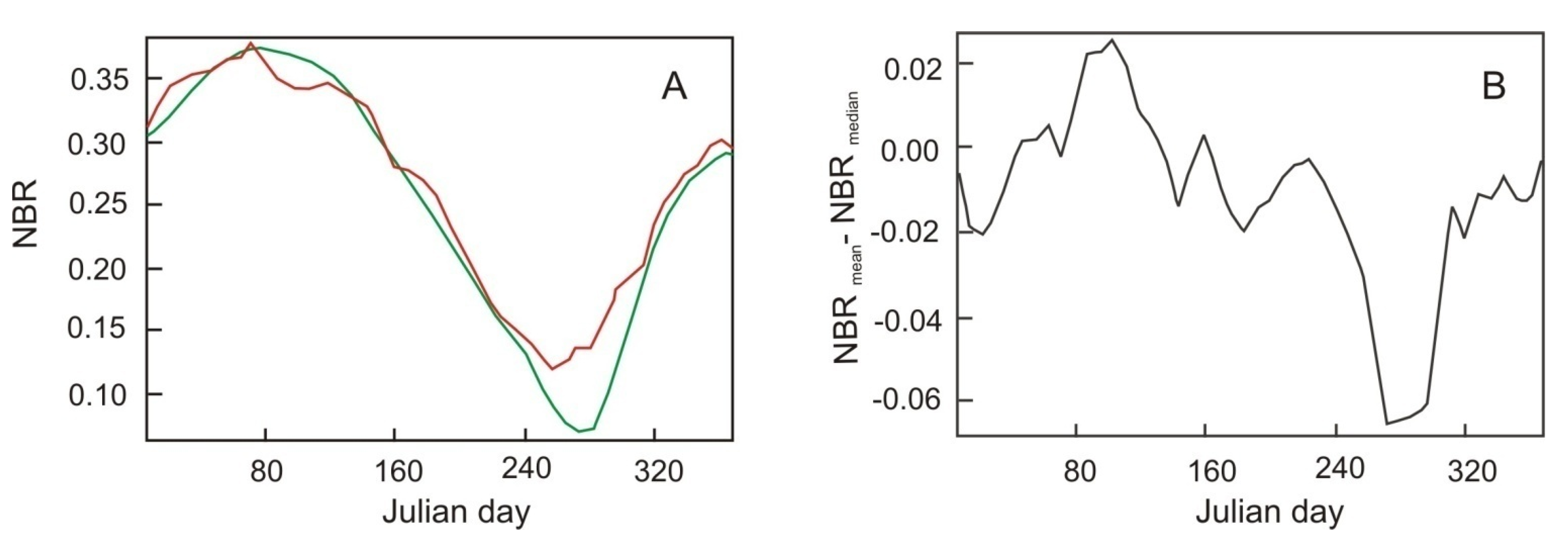
The differences between the phenological curves obtained by the mean and median are usually very small. The main differences occur in the maximum and minimum points, where the median values tend to be less pronounced than mean values (Figure 16). This characteristic demonstrates that the median nullifies the interference of extreme values such as the presence of clouds, shadows, and burned areas. However, the mean temporal curve has a more smoothed contour than the median curve. The interannual curves from the trimmed mean show an intermediate behavior between the mean and median curves. The annual information of the time series are subtracted from the average interannual curves generating the deviation images. The fire event changes the cyclical behavior of temporal curve causing a drop in the NBR values, which is marked in the deviation image by lower values (dark areas).

Figure 16. Comparison between the mean annual curve (green line) and (A) median annual curve (red line), and (B) difference curve (mean–median).

Figure 16. Comparison between the mean annual curve (green line) and (A) median annual curve (red line), and (B) difference curve (mean–median).

4.2.2. Threshold Value for Burned-Area Detection Using Deviation Images

The accuracy assessment to detect the optimum threshold values was performed between the reference data from Landsat-TM classification and MODIS-NBR deviation images from the methods of median, mean and alpha-trimmed mean (alpha equal to 0.1, 0.2, 0.3, and 0.4). The alpha-trimmed mean is a symmetric trimming, which adopts the central part of the ordered array defined by the alpha parameter ranging from 0 (mean) to 0.5 (median). The reference images were the same adopted in the standardized-image analysis on 25 October 2007 and 29 September 2010 in order to facilitate comparison among the methods.

Table 1 compares the accuracy indices (Overall Accuracy and Kappa Coefficient) of the optimum threshold values between the reference data and the deviation images from the different central tendency methods. The accuracy values among the methods are very close. The trimmed mean using alpha equal to 0.4 achieved the best result with Overall Accuracy of 86.385 and Kappa coefficient of 0.7188.

Table 1. Overall Accuracy and Kappa Coefficient for the optimum threshold values between deviation image (mean, trimmed mean and median) and the reference data (Landsat-TM classification).

Deviation-Image Method	Overall Accuracy	Kappa Coefficient
Mean	86.118	0.7156
Trimmed mean(alpha = 0.1)	86.385	0.7188
Trimmed mean(alpha = 0.2)	86.264	0.7183
Trimmed mean(alpha = 0.3)	86.259	0.7172
Trimmed mean(alpha = 0.4)	86.191	0.7157
Median	86.137	0.7110

Table 1. Overall Accuracy and Kappa Coefficient for the optimum threshold values between deviation image (mean, trimmed mean and median) and the reference data (Landsat-TM classification).

Deviation-Image Method	Overall Accuracy	Kappa Coefficient
Mean	86.118	0.7156
Trimmed mean(alpha = 0.1)	86.385	0.7188
Trimmed mean(alpha = 0.2)	86.264	0.7183
Trimmed mean(alpha = 0.3)	86.259	0.7172
Trimmed mean(alpha = 0.4)	86.191	0.7157
Median	86.137	0.7110

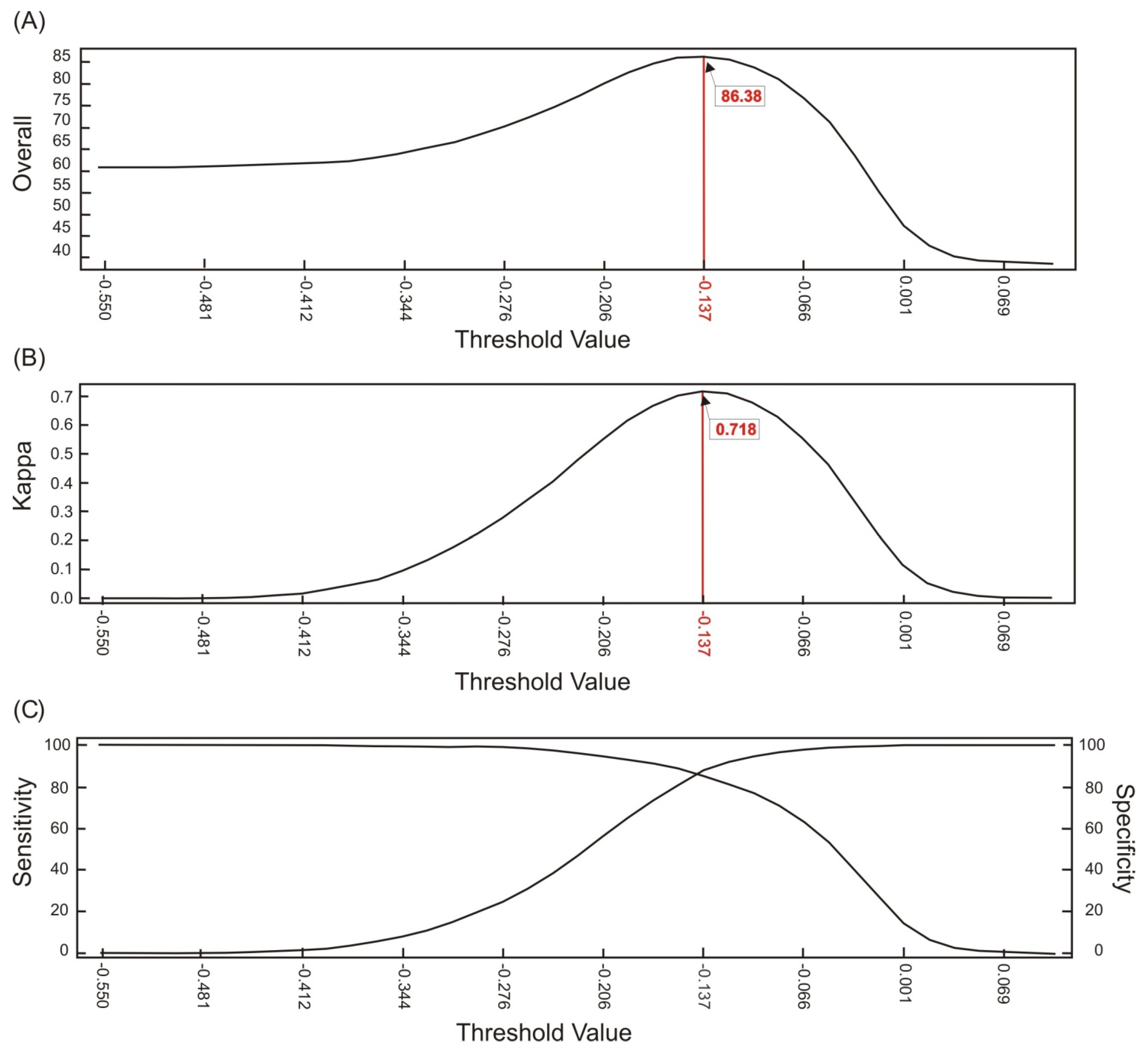
Figure 17 showed the accuracy assessment curves between deviation image from the interannual trimmed mean (alpha = 0.1) and the reference data. The accuracy indices determine an optimum threshold value of 0.137. The accuracy values of the deviation-image methods are slightly lower than the standardized time series method.

Figure 17. Identification of the optimal threshold values for burned-area detection from the deviation images using trimmed mean interannual phenology (alpha = 0.1). The accuracy assessment curves refer to the following indices: (A) Overall accuracy, (B) Kappa coefficient, and (C) Sensitivity-Specificity pair.

Figure 17. Identification of the optimal threshold values for burned-area detection from the deviation images using trimmed mean interannual phenology (alpha = 0.1). The accuracy assessment curves refer to the following indices: (A) Overall accuracy, (B) Kappa coefficient, and (C) Sensitivity-Specificity pair.

The removal of the seasonal component allows emphasizing the fire effects. Usually, the fire event exhibits a lower value than that predicted by central-tendency curves. Thus, a negative anomaly with asymmetrical shape characterizes the burned area. Initially, the fire event presents a sharp drop in the deviation values from NBR, which recovers slowly from the regrowth vegetation to achieve the foregoing cyclic values. Figure 18 shows a temporal curve of deviation using the median interannual values with three negative anomalies of fire events from threshold value.

Figure 18. (A) Temporal curve of deviation from the trimmed mean interannual phenology (alpha = 0.1) with three negative anomalies of fire events; (B) deviation image acquired on Julian day 289 in 2003; (C) Julian day 281 in 2007; and (D) Julian day 281 in 2012. The red dot on the deviation images marks the location of the temporal curve.

Figure 18. (A) Temporal curve of deviation from the trimmed mean interannual phenology (alpha = 0.1) with three negative anomalies of fire events; (B) deviation image acquired on Julian day 289 in 2003; (C) Julian day 281 in 2007; and (D) Julian day 281 in 2012. The red dot on the deviation images marks the location of the temporal curve.

4.3. Results of the Seasonal Differencing

The seasonal-differencing method, widely used in burned-area detection, was also applied in order to be compared with the proposed methods. This procedure showed the loss of a year in the time series after the difference calculation. The optimal threshold-value definition was obtained using the same procedure and reference images applied to the previous methods.

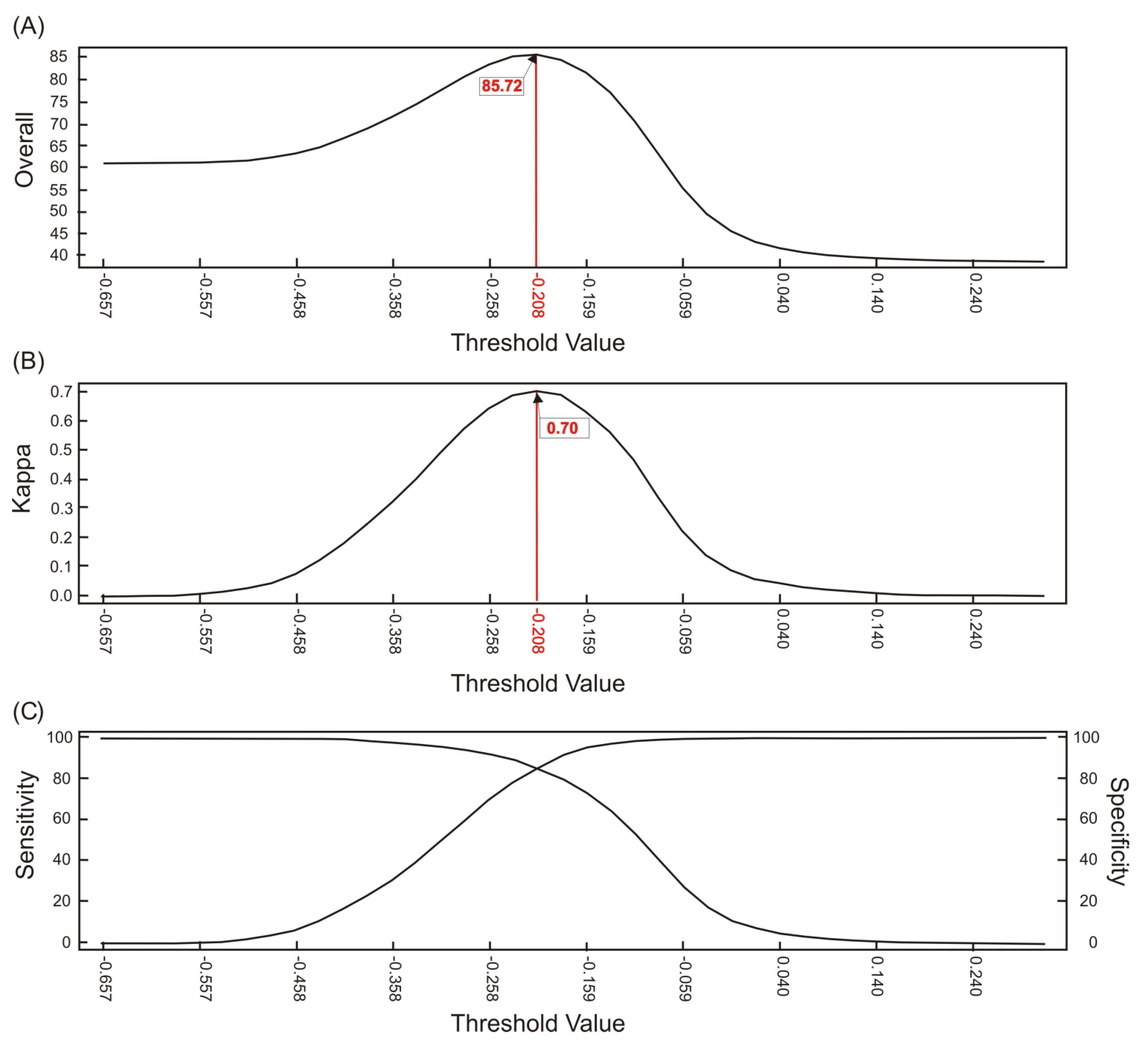
Figure 19 demonstrates the accuracy curves, where the optimal threshold value is 0.208 having a Kappa Coefficient of 85.72 and Overall Accuracy of 0.70. The optimal threshold value was applied in the temporal series obtaining the mask series of burned-areas.

Figure 19. Identification of the optimal threshold values for burned-area detection from the deviation images using seasonal differencing. The accuracy assessment curves refer to the following indices: (A) Overall accuracy, (B) Kappa coefficient, and (C) Sensitivity-Specificity pair.

Figure 19. Identification of the optimal threshold values for burned-area detection from the deviation images using seasonal differencing. The accuracy assessment curves refer to the following indices: (A) Overall accuracy, (B) Kappa coefficient, and (C) Sensitivity-Specificity pair.

4.4. Method Comparison

4.4.1. Analysis in the Fire Event

In the periods of the fire events, the different methods presented very close accuracy values considering the reference data from the Landsat TM images (Figure 14, Figure 18 and Figure 19). In the best-threshold detection, the standardized image method had the best result (Kappa coefficient of 0.75 and Overall Accuracy of 87.73), followed by the interannual phenological deviation method using the trimmed mean (alpha = 0.1) (Kappa coefficient of 0.71 and Overall Accuracy 86.38), and finally the worst result was for the seasonal difference method (Kappa coefficient of 0.70 and Overall Accuracy of 85.72).

In addition, a validation using an independent set from Landsat data was utilized to quantify the effectiveness of the proposed methods. The available images from the TM Landsat sensor had less extensive burned areas than those used in defining the threshold value. The Landsat TM data on 22 September 2004 (Julian day 266) contains a burned area of 75 km² that corresponding to 4.5% of the used image. Therefore, several smaller fragments of the burned area were classified and compared with the burned area masks obtained by different methods. Accuracy results are slightly different to the identification step of the optimal threshold values, displaying higher Overall Accuracy and lower Kappa coefficient. The ordination among the methods remained, in which the standardized image method had the best result with Kappa coefficient of 0.66 and Overall Accuracy of 97. The interannual phenological deviation method using the trimmed mean (alpha = 0.1) obtains Kappa coefficient of 0.63 and Overall Accuracy of 96.79. Lastly, the seasonal difference method had Kappa coefficient of 0.55 and Overall Accuracy of 96.46.

Accuracy differences between the phases of best-threshold detection and independent validation have a potential source in the burned-area size. Note that difference between spatial resolution of the MODIS and Landsat TM images increases the divergence of burned-area mapping using the smallest fragments. Smaller fragments have proportionately more pixels in the edge region, which is more susceptible to errors resulting from the fit between the spatial resolutions. In contrast, large fragments have a higher percentage of internal pixels and thus show fewer propensities to errors due to edge effects and spatial resolution. Therefore, the lower efficiency described by Kappa coefficient is expected considering the decrease in the fragment. The significant increase in the free-fire areas provides an increase in the Overall Accuracy.

The similar accuracy values among the tested methods during the same period were expected, since the reduction of the resulting value for burned areas is very noticeable in all methods. However, the major differences among the methods were in the mask series of burned areas that are usually outside the fire-event period and caused by errors in the baseline adjustment.

4.4.2. Baseline-Adjustment Error

The seasonal differencing and interannual phenological deviation methods are more susceptible to errors because these presuppose the presence of a previous baseline, which are not always fitted to the temporal data in a meaningful and efficient way. Three main situations cause the baseline-adjustment error in these two methods: (a) delay of the dry season, (b) anomalous values of NBR, and (c) other changes in land use and land cover both anthropogenic (e.g., agriculture, urbanization) as natural (e.g., landslide, inundation).

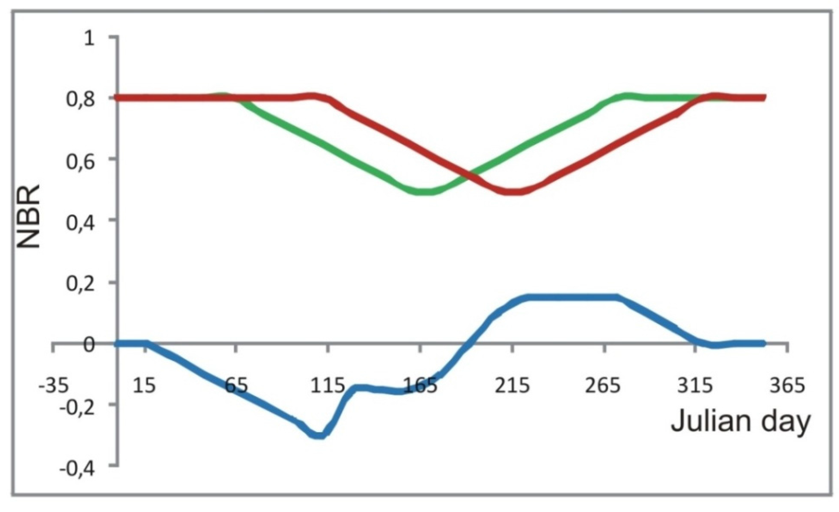
Figure 20 shows schematically the effect caused by the delay of the dry season. The subtraction line (green line) falls significantly only because of the delay of phenology cycle, not being correlated to the fire effect. This error type from the climatic factors is concentrated in a particular period of the year and generates extensive features.

The error caused by anomalous NBR values may be derived from a noise or a vegetation change. This error is very common in both methods and is scattered throughout the time series. It may be present in one of the methods and absent in the other due to their baseline differences. The seasonal difference method is a change detection technique that besides the burned areas, emphasizes other changes in the earth’s surface. In this way, the dNBR values in the agricultural areas generate false-positive features that are mistaken for fire events. The baseline adjustments in fire-event studies lead to an overestimation of burned area. In order to emphasize this difference, both temporal (z-profiles) and spatial (images) comparative analyses were performed.

Figure 20. Baseline-adjustment error from the delay of the dry season, where the green line is the time series, the red line is the time series in a previous year, and the blue line isa subtraction between the two. The high NBR values are incompatible with burned areas, although the seasonal difference presents a significant decrease of values.

Figure 20. Baseline-adjustment error from the delay of the dry season, where the green line is the time series, the red line is the time series in a previous year, and the blue line isa subtraction between the two. The high NBR values are incompatible with burned areas, although the seasonal difference presents a significant decrease of values.

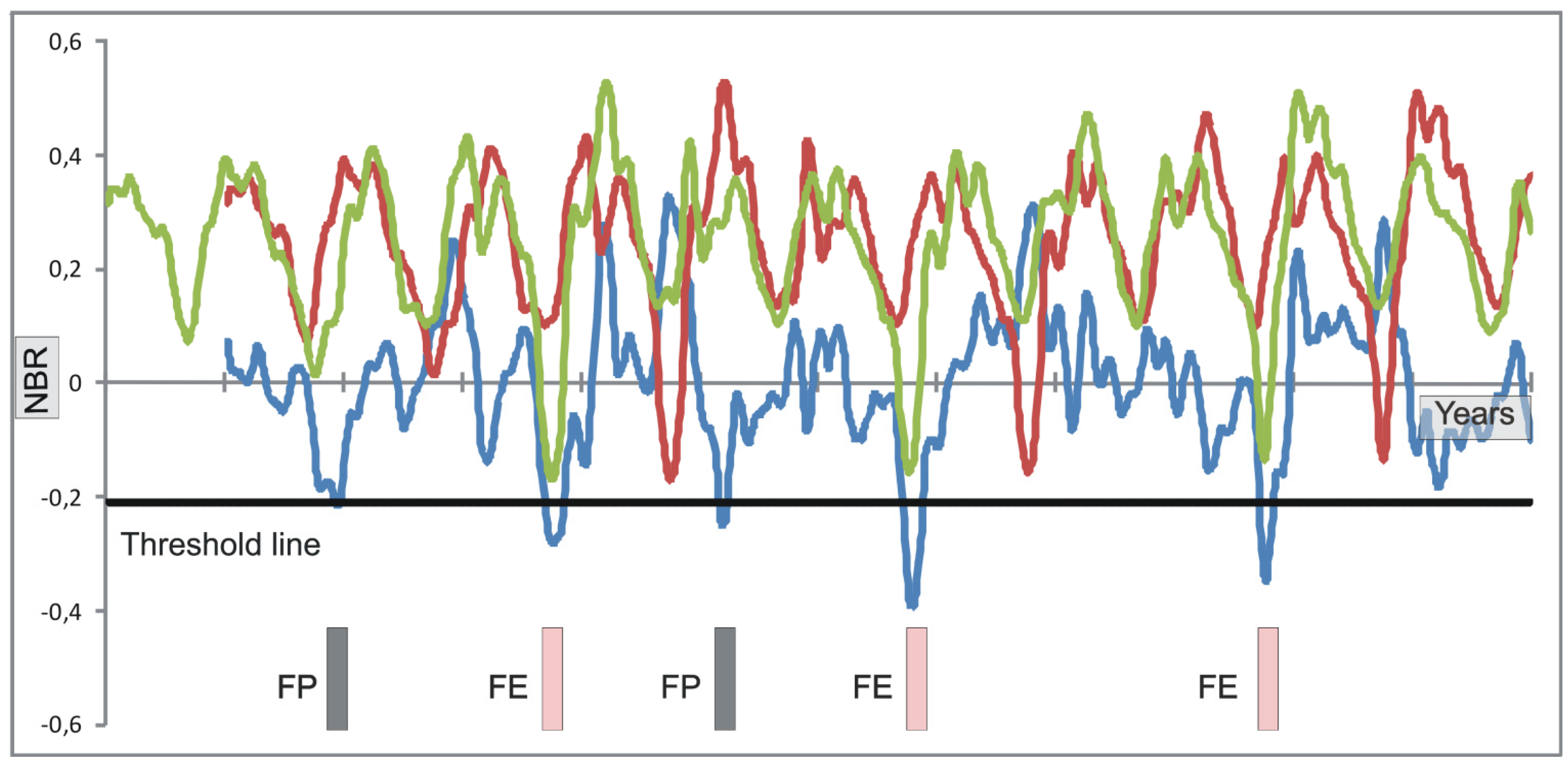
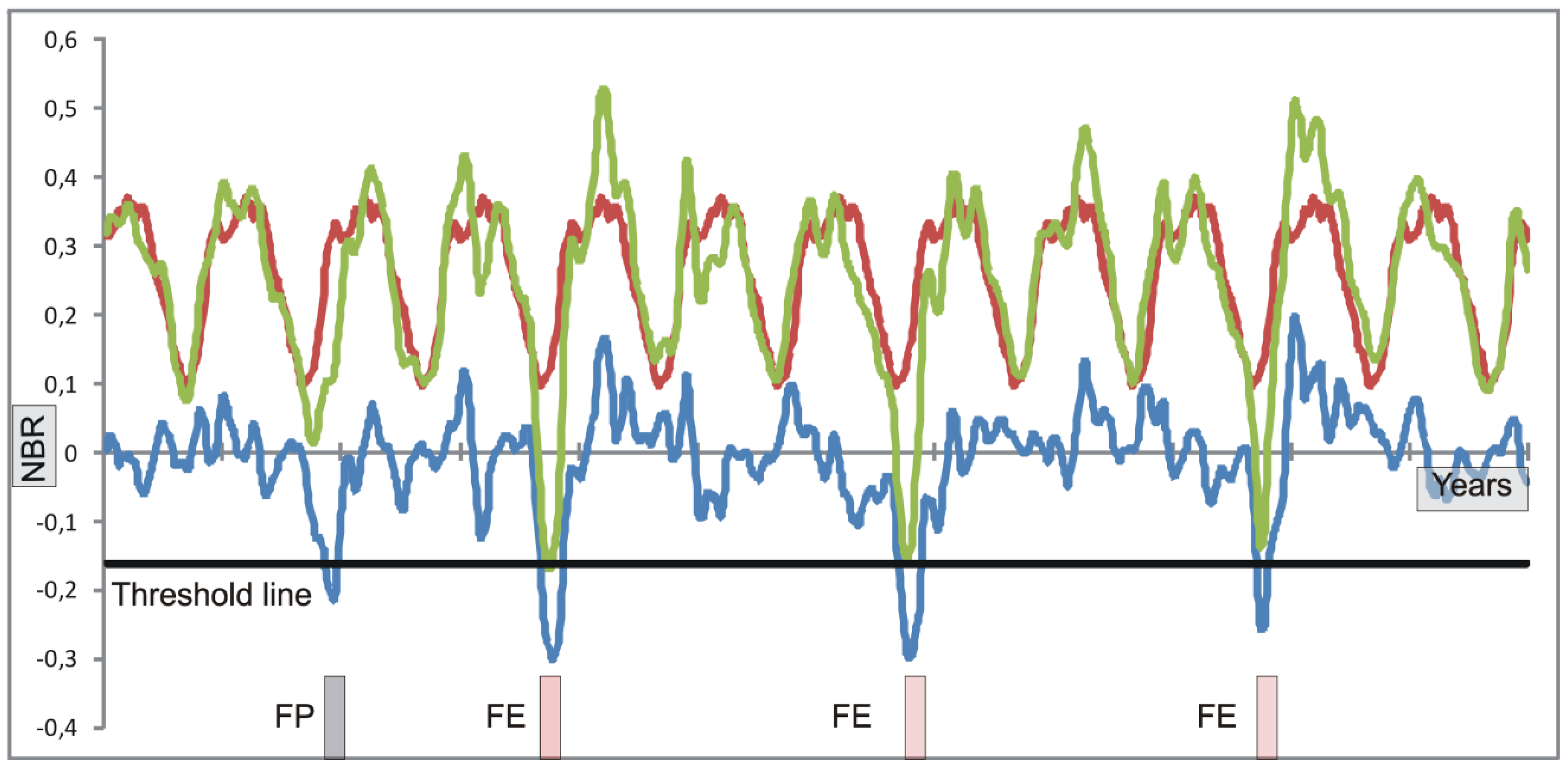
Figure 21 shows the seasonal-difference curve (blue line), MODIS-NBR time series (green line) and time series with a one-year delay (red line). The dNBR curve had five fire events, two of which are baseline-adjustment errors and three correspond to the burned events (i.e., 40% of fire-event error). The actual burned areas were mapped correctly in accordance with the foregoing analysis that shows high Overall Accuracy and Kappa coefficient on fire events. The main issue is the mistaken detection of more fire events that really happened in the time series. The first error was due to a delay of the rainy season. The second error occurs during a rainy period and is not tied to a fall in the NBR value in the time series, revealing an error in the demarcation. 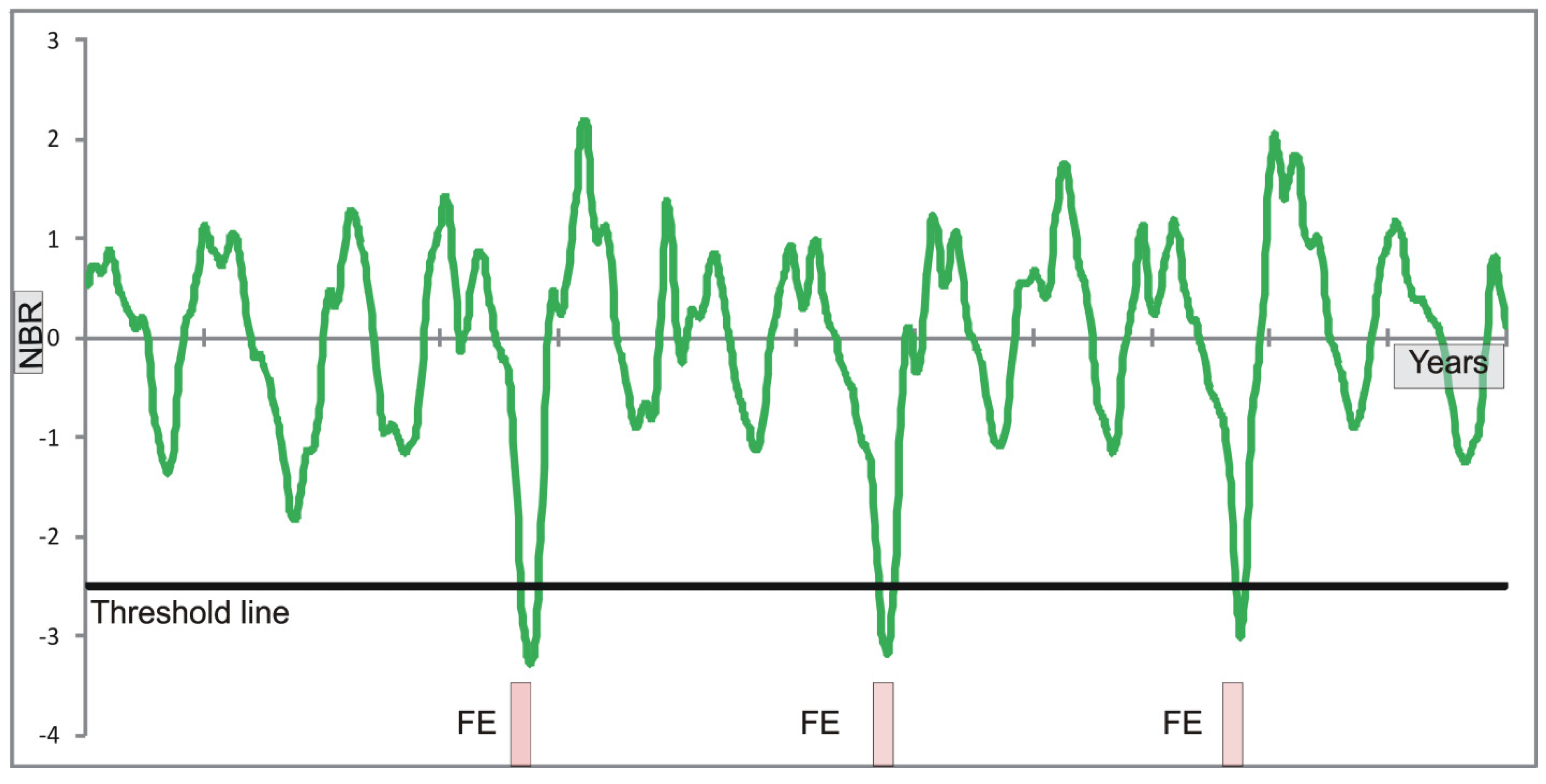Figure 22 shows the burned-area detection in the same time series (green line) considering the deviation from the median annual phenology (red line). The interannual-deviation curve (blue line) detected the same three fire events, but remained a baseline-adjustment error. The standardized time series showed the best results, i.e., error-free (Figure 23).

Most baseline-adjustment error occurs in conditions of high NBR values (not consistent with the burned areas) and low dNBR and deviation values (Figure 21 and Figure 22). In contrast, true burned-areas have low values for NBR, dNBR and deviation. This distinct pattern allows establishing an independent algorithm for error detection. As a precaution, low dNBR on rainy period preceded by fire events during the dry season (seven months earlier) were discarded as being baseline-adjustment errors. However, the savannas have a rapid recovery of vegetation after the fire event (especially grass species) and achieve normal NBR values in the rainy season. In summary, an estimative of baseline-adjustment error can be computationally accomplished through the following constraints: (a) burned areas detected by seasonal differencing or deviation image with high NBR values, and (b) absence of burned areas during the last months. 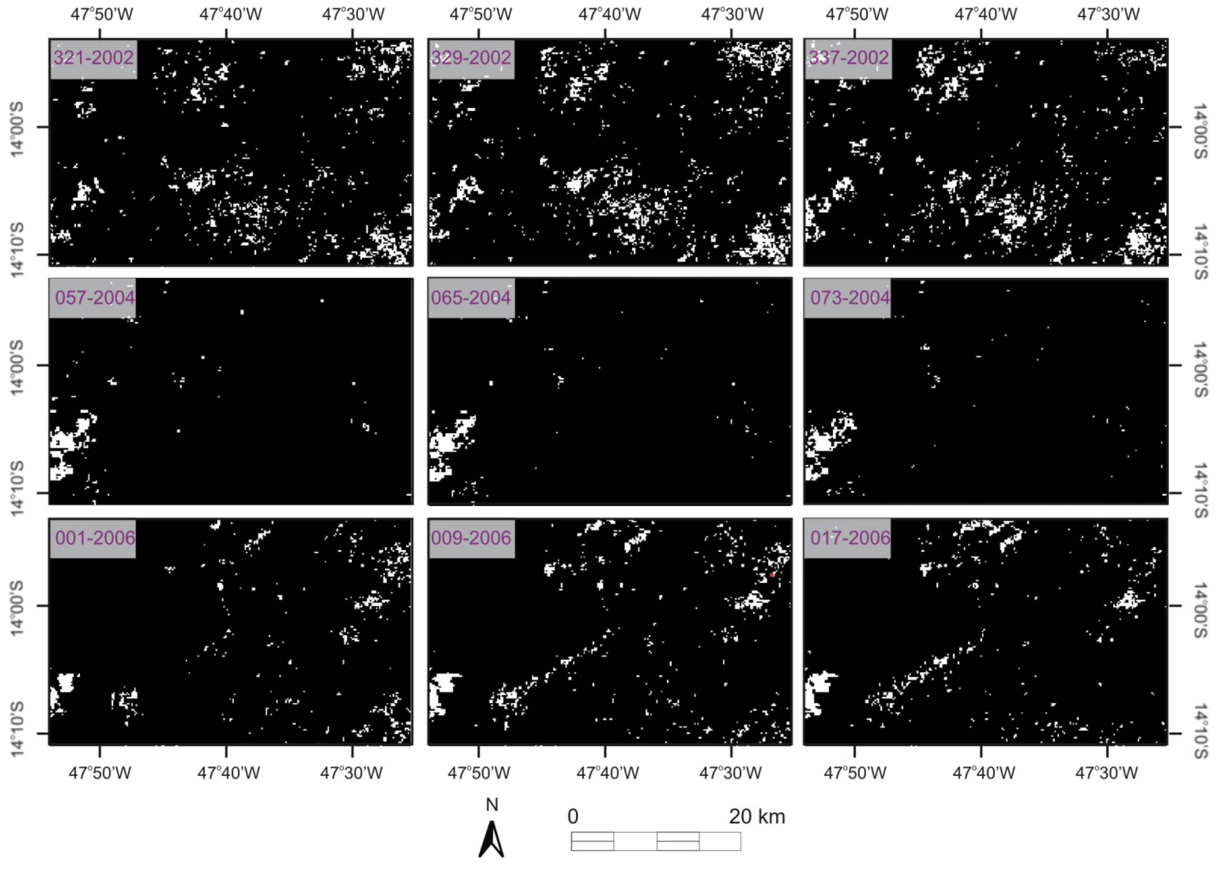Figure 24 shows the mask images related to baseline-adjustment errors with high NBR values using seasonal differencing. The dates are all concerning the rainy season when fire events do not occur. Most errors are persistent over time, occurring in the successive images.

Figure 21. Detection of burned areas using the seasonal difference method, where the MODIS-NBR time series is the green line, the time series with a one-year lag is the red line, the dNBR curve is the blue line and the threshold line is the black line. Fire events (FE) and false positive (FP) are marked on the bottom of the chart.

Figure 21. Detection of burned areas using the seasonal difference method, where the MODIS-NBR time series is the green line, the time series with a one-year lag is the red line, the dNBR curve is the blue line and the threshold line is the black line. Fire events (FE) and false positive (FP) are marked on the bottom of the chart.

Figure 22. Detection of burned areas using the interannual phenological deviation, where the MODIS-NBR time series is the green line, the time series with a one-year lag is the red line, the dNBR curve is the blue line and the threshold line is the black line. Fire events (FE) and false positive (FP) are marked on the bottom of the chart.

Figure 22. Detection of burned areas using the interannual phenological deviation, where the MODIS-NBR time series is the green line, the time series with a one-year lag is the red line, the dNBR curve is the blue line and the threshold line is the black line. Fire events (FE) and false positive (FP) are marked on the bottom of the chart.

Figure 23. Detection of burned areas using the standardized time series (green line). Threshold line is the black line. Fire events (FE) and false positive (FP) are marked on the bottom of the chart.

Figure 23. Detection of burned areas using the standardized time series (green line). Threshold line is the black line. Fire events (FE) and false positive (FP) are marked on the bottom of the chart.

Figure 24. Mask images of the false-positive features with high NBR value. The date is expressed in Julian day and year.

Figure 24. Mask images of the false-positive features with high NBR value. The date is expressed in Julian day and year.

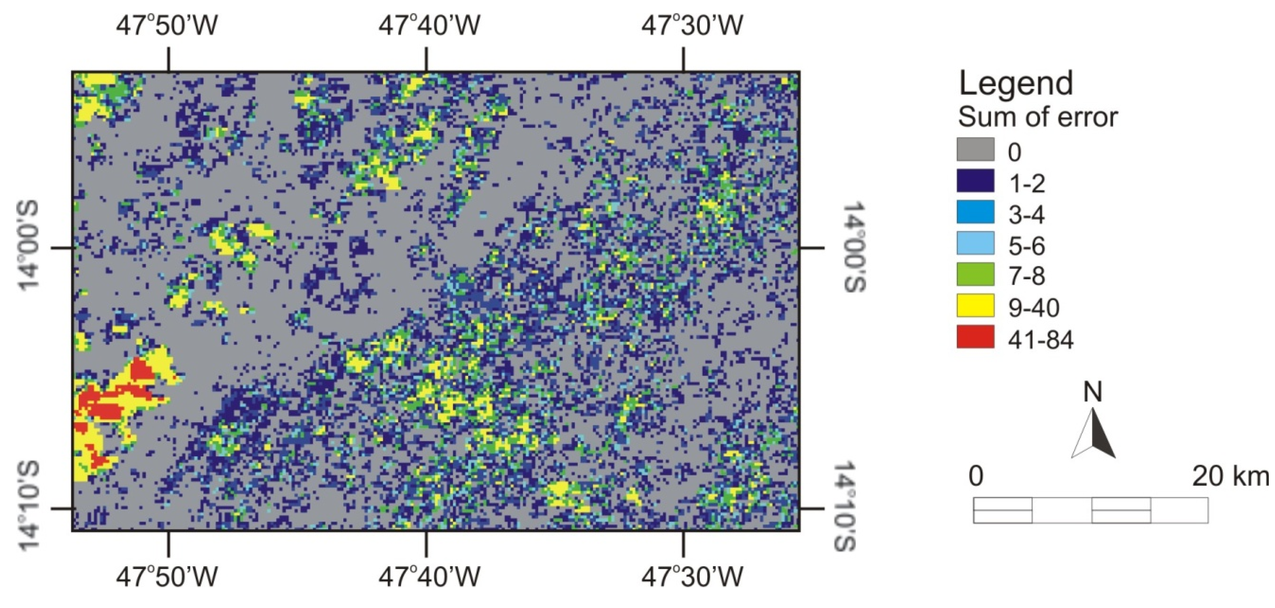
The sum of the error masks in the period 2002 to 2012 shows an approach to assess the importance of baseline-adjustment error in the temporal series. The error-summation image from seasonal differencing has a mean occurrence of 2.18, standard deviation of 5.43 and varies from 0 to 84 (Figure 25). The main errors are located in the southwest part of the image at a location outside the park with the presence of agricultural cultivation (demarcated by red color in Figure 25). In this area, the agricultural changes cause a strong influence on dNBR values that persists for several days.

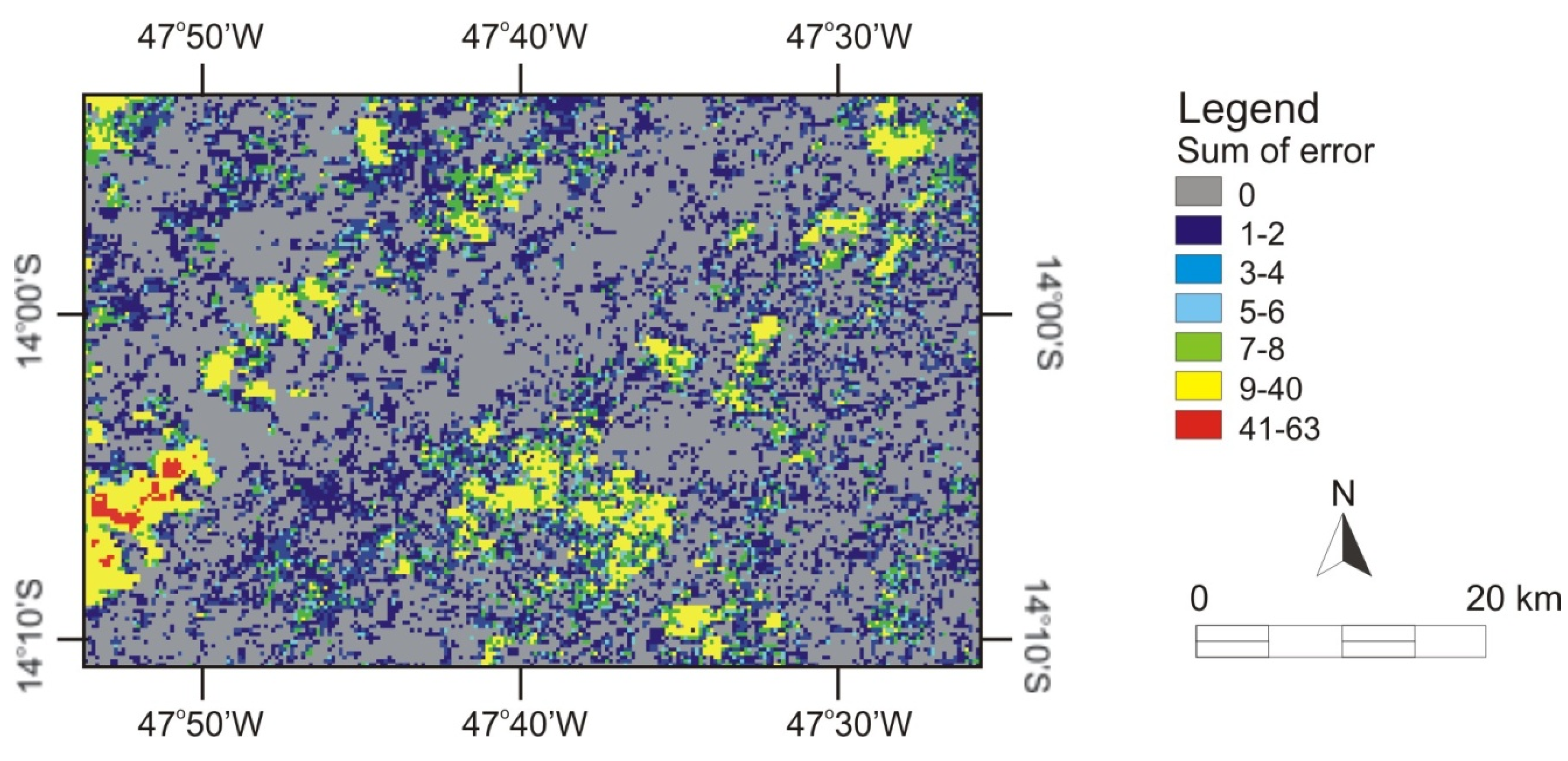
The error-summation image from interannual phenological deviation has a mean occurrence of 2.42, standard deviation of 5.07 and varies from 0 to 63 (Figure 26). Despite that the errors from both methods using baseline possess a similar spatial distribution, the intensities are different. The error-summation images point out that the standardized time series method obtains a large advantage over the other two methods for not having this type of error.

Figure 25. Error-summation image from seasonal differencing in the period 2002 to 2012.

Figure 25. Error-summation image from seasonal differencing in the period 2002 to 2012.

Figure 26. Error-summation image from interannual phenological deviation in the period 2002 to 2012.

Figure 26. Error-summation image from interannual phenological deviation in the period 2002 to 2012.

4.5. Program

The methods discussed are available in the Abilio software developed in C++ language. The main functions of the program are organized in the main window interface, which contains the image input boxes, method modules and image display. The program reads general raster data stored as an interleaved binary stream of bytes in the Band Sequential Format (BSQ). Each image is accompanied by a header file in ASCII (text) containing information to read data file, such as: sample numbers, line numbers, bands, interleave code (BSQ) and data type (byte, signed and unsigned integer, long integer, floating point, 64-bit integer, unsigned 64-bit integer). This configuration combining image and header file allows versatility in the use of different image formats. When the user tries to open an image without the header file, an interface requesting the necessary information about the input image structure automatically appears.

In the software, the following modules for time-series normalization were added: (1) standardized time-series image method; (2) phenological deviation image method; and (3) traditional method of seasonal differencing. These methods consider as input data the NBR-MODIS time-series. In cases of using the phenological deviation method, the number of the image by year and the type of central tendency value (mean, median and trimmed median) are also required. The standardized time-series and phenological deviation images have the same dimension as the input time-series images, while a seasonal difference image experiences a reduction of its size in a year. Additionally, a module for generating mask series burned areas was also implemented, having as input the normalized images.

All inputs and results are shown in the File List, so it is possible to visualize them by choosing “Gray Scale” or “RGB” composite. The display interface provides basic functions for image visualization such as zoom areas and pixel values. Moreover, the results (output files) can be read from other software.

5. Discussion

The pre-/post-fire differencing from NBR index is widely applied to burned-area detection. The vast majority of studies utilize this methodology adopting images of discrete times that are previously selected for a specific analysis, i.e., using pre-fire images constituted by the pixels unaffected by the fire or noises. This condition usually guarantees high quality for the dNBR index [13,19,24,34,84]. Nevertheless, this procedure for discrete data over time becomes different when applied to the complete time series. In this new approach, all images are used together, which favors the error propagation.

The researches of burned-area detection using time series define a dNBR threshold, which classifies as burned when it exceeds the pixel value [74]. All images in the time series adopts the same predetermined threshold. Veraverbeke et al. [74] establish a relatively low threshold to minimize the omission error in low severity pixels and consider the persistence of the post-fire NBR drop during five consecutive observations in time. We suggest an algorithm to establish the best threshold value considering a reference mapping. This method reduces subjectivity and adjusts the threshold value in order to provide the best accuracy indices. As in the previously adopted procedure, the threshold value is applied to the complete time-series. Whereas only one threshold is used, the algorithm allows you to attach multiple images in order to achieve a threshold value from different imaging conditions. The combined analysis of multiple images to determine the threshold value decreases the site dependence. Despite the advances in the threshold-value detection, further research should be done to improve and consider specific situations.

The seasonal differencing method may introduce errors from phenological changes due to climatic constrains. These variations are more pronounced in semi-arid environments such as the Cerrado biome. Rainfall is determinant in phenological responses of the Cerrado vegetation, because it stimulates green-up onset and determines the duration of growth and flowering of plants [83,85]. Therefore, variations of the beginning and end of the rainy season changes dNBR values because they cause a gap between the phenological curves of the two subsequent years. In this respect, Diaz-Delgado and Pons [86] adopt the difference between burned area and control pixels of unburned area within the same image. However, this procedure has limitations when applied on a large scale because of the need for intensive fieldwork to select relevant control pixels. Moreover, the reference is an average value and does not depict the heterogeneity of the burned area. Lhermitte et al. [36] tries to solve this problem from a selection method of pixel control, which considers the similarity between the time series of burned pixels and the time series of its surrounding unburned pixels for a pre-fire year. However, other factors that are not completely controlled can influence the behavior of the index from the neighboring pixels with unburned areas. Very large burned areas can overcome different environments, especially in savanna, making it difficult to establish the pixel control points. The method is not completely automatic and is in need of supervision. Spatial variability of soil and hydrologic properties can also result in neighboring pixels with different environmental behaviors in relation to analyzed pixel.

Three major effects can be considered for the seasonal differencing. First, the time series lost one year. Second, seasonal differencing increased the presence of noise, since interference affects both the year under analysis and the next year, when it is used as the factor to be subtracted. Third, variations of the phenological (e.g., rain delay) and cropping cycles can cause changes in the seasonal-difference values.

In this study, the two proposed methods have the advantage to be fully automated and restricted to the pixel information. The proposed methods and seasonal differencing have similar accuracy for large fire events. On this occasion, the NBR values are considerably lower in all methods facilitating its detection. This explains the success of dNBR for bi-temporal images related to fire events as shown by the various articles [19,24,34]. The accuracy values in this study are consistent with other researches for fire detection using MODIS data.

However, these methods are significantly different over the entire time series. The interannual phenological deviation method also presented susceptibility to the presence of errors because it uses baseline. Moreover, this method requires a long stable period to achieve a consistent central tendency value, becoming more restricted to natural environments.

In contrast with the traditional approach, the standardized time-series method eliminates this interference effect. This method provides a new solution to the problem, not using baseline that is subtracted from the time series. Thus, the method does not add false information or noise to the temporal data. Instead, the proposed method performs a z-score standardization, which does not alter the relative position among the points within the temporal curve and provides equivalence for the low values of the burned areas in the different environments. This new method is very helpful in maintaining a coherent and common structure of the data, avoiding adding unnecessary information.

6. Conclusions

Typically, the processing for the burned area detection is a combination of a spectral index and a data normalization using seasonal differencing. Many studies focus on the comparison between spectral indices (e.g., NBR, NDVI, among others). However, the seasonal difference method applied to long-term measured time series is very susceptible to false positives errors from the mismatch between the successive annual phenological curves. Therefore, a sharp fall in the dNBR occurs at various points of the temporal curve that are not related to fire events. Despite the problems created by the seasonal difference, no other normalization method has been proposed.

This research proposes the use of two new procedures for the normalization of time series. The tests were performed in savanna areas, composed of different vegetation and environments, which hinders the burned-area mapping. All methods perform well for fire events, due to the significant fall in NBR values. The standardized method has slightly better results, while the seasonal difference represents the worst results. However, the seasonal difference and phenological deviation methods introduce many false positive errors throughout the entire time series (disregarding the fire event), because of the incompatibility between the input data and baselines (previous year or average interannual). This type of error is intensified by the change between the dry and rainy seasons. The standardized time series provide a new solution to the problem; maintaining the relative positions inside the time series. The points of the time series undergo offset and gain changes by constant values (mean and standard deviation, respectively). The procedure afforded compatibility among the time series of different environments, enhancing the burned areas without introducing errors. Thus, the proposed method is appropriate for automatic image processing of the long-term time series for burned-area detection.