A New Look at Image Fusion Methods from a Bayesian Perspective

Abstract

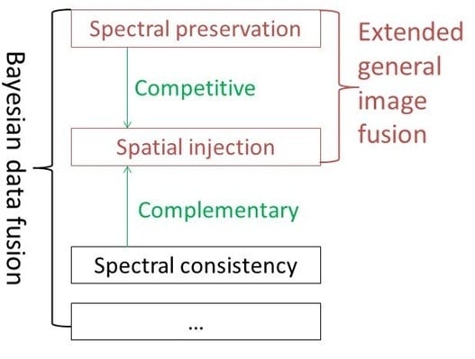
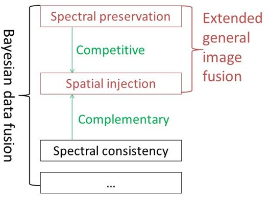
Component substitution (CS) and multi-resolution analysis (MRA) are the two basic categories in the extended general image fusion (EGIF) framework for fusing panchromatic (Pan) and multispectral (MS) images. Despite of the method diversity, there are some unaddressed questions and contradictory conclusions about fusion. For example, is the spatial enhancement of CS methods better than MRA methods? Is spatial enhancement and spectral preservation competitive? How to achieve spectral consistency defined by Wald et al. in 1997? In their definition any synthetic image should be as identical as possible to the original image once degraded to its original resolution. To answer these questions, this research first finds out that all the CS and MRA methods can be derived from the Bayesian fusion method by adjusting a weight parameter to balance contributions from the spatial injection and spectral preservation models. The spectral preservation model assumes a Gaussian distribution of the desired high-resolution MS images, with the up-sampled low-resolution MS images comprising the mean value. The spatial injection model assumes a linear correlation between Pan and MS images. Thus the spatial enhancement depends on the weight parameter but is irrelevant of which category (i.e., MRA or CS) the method belongs to. This paper then adds a spectral consistency model in the Bayesian fusion framework to guarantee Wald’s spectral consistency with regard to arbitrary sensor point spread function. Although the spectral preservation in the EGIF methods is competitive to spatial enhancement, the Wald’s spectral consistency property is complementary with spatial enhancement. We conducted experiments on satellite images acquired by the QuickBird and WorldView-2 satellites to confirm our analysis, and found that the performance of the traditional EGIF methods improved significantly after adding the spectral consistency model.

1. Introduction

With the development of science and technology, remote sensing data have exhibited explosive growth trends for multi-sensor, multi-temporal and multi-resolution characteristics. However, there are contradictions between the resolution limitations of current remote sensing systems and the increasing need for high-spatial, high-temporal and high-spectrum resolutions of satellite images [1]. One limitation is the spectral and spatial resolution tradeoff, as more than 70% of current optical earth observation satellites simultaneously collect low-spatial resolution (LR) multispectral (MS) and high-spatial resolution (HR) panchromatic (Pan) images [2]. This tradeoff will survive in forthcoming hyperspectral and MS sensors such as WorldView-3, EnMAP, PRISMA and HyspIRI [3]. Based on information fusion theory, satellite image fusion has been proposed to handle these limitations [4,5]. Pansharpening, which is a spatial and spectral fusion method, focuses on enhancing LR MS images using the Pan image to obtain both high-spatial and high-spectral resolution images [6]. Despite the variety of current pansharpening methods, they can generally be classified into component substitution (CS) and multi-resolution analysis (MRA) methods. Both the CS and MRA methods have been generalized into the extended general fusion framework (EGIF) [7,8].

Many studies have focused on comparing and reviewing these methods [4,5,8,9,10,11,12,13,14,15,16,17,18,19,20,21,22,23] and had several common findings. First, among the CS methods, the Gram-Schmidt (GS) algorithm [24] was found to be the best in terms of spectral preservation and spatial injection [2,7,25]. Second, among the MRA methods, the generalized Laplacian pyramid (GLP) has been shown to present advantages, as it can adapt to the sensor point spread function (PSF) [15,26,27,28]. Finally, a current trend of pansharpening methods is to preserve the spectral information of the original MS images. This preservation is accomplished in two ways. First, CS methods are either adopted on their own to create an ideal intensity by accounting for the spectral response functions or using linear regression technology [25,29,30,31], or combined with MRA methods [32,33,34]. Second, MRA methods are adopted to modulate high frequencies using global or local injection models [23,35] such as AABP (an acronym formed from its authors’ initials, i.e., Aiazzi, Alparone, Baronti and Pippi [36]), high-pass modulation (HPM) [37], context-based decision (CBD) [15,28], enhanced CBD [27], proportional additive wavelet LHS (intensity-hue-saturation) [38] and Model 3 (M3) [39]. Despite these findings, pansharpening remains a source of confusion and unaddressed questions, which are listed as follows.

Question 1: The relationship between the CS and MRA methods is not well understood. According to the EGIF, the only difference between CS and MRA methods is how to extract the spatial details. And the injection models to control the spatial detail injection amount utilized by the CS and MRA methods are similar [7]. Thus the enhancement of CS methods should be comparable to that of MRA methods. However, there are some studies which observed that the spatial enhancement of CS methods is larger than that of MRA methods [27,40,41,42].

Question 2: There is a contradicting conclusion on the existence of the spatial enhancement and spectral preservation tradeoff in the fused images. Many CS method developers believed this tradeoff and tried to balance this tradeoff by introducing weight parameters to control the spatial injection [41,43,44]. Some MRA method developers implicitly assumed this tradeoff as they used optimization technologies with competitive objectives, i.e., to maximize the spatial similarity to the Pan image and the spectral similarity to the up-sampled MS images [45] to determine the best injection model [45,46,47]. Furthermore, in the MRA and CS comparison studies, researchers have found that although the spatial enhancement of CS methods is better than that of MRA methods [40,41,42], the spectral preservation of the former is worse. This indeed enhances the fidelity of the tradeoff quality in fused images [17,48,49]. However, Thomas et al. [10] challenged the existence of the tradeoff by stating that “this tradeoff is a consequence of the use of certain tools and not an a priori compulsory”. They claimed that it cannot be reduced to the spatial information of its associated spectral information in an image. As such, the question remains: does the tradeoff really exist?

In fact, the question 2 originates from that the implicit spectral preservation definition in current pansharpening algorithms is improper. In pansharpening algorithms, the spectral preservation is defined to be as identical as possible to the up-sampled MS images. We will prove that from a Baysian perspective that all the EGIF methods have used the MS image as prior knowledge to preserve spectral information although only a few have explicitly stated that. For example, some intensity-hue-saturation-based (IHS-based) methods for spectral preservation have been developed by maintaining the saturation of the up-sampled MS images [29,41,50]. Some MRA methods indicate that if the Pan and MS images exhibit a low correlation, the up-sampled images can be used as a fused product for preserving spectral information [10,28,47]. In contrast, as observed by Wald et al. [51], spectral consistency infers that any synthetic image degraded to its original resolution with respect to the sensor PSF should be as identical as possible to the original image [51,52]. Recently, Chen et al. [53] have noticed the upsampled MS image (used in EGIF) is not as accurate as the original MS image (defined by Wald) for preserving the spectral information. The questions are how to guarantee spectral consistency with Wald’s definition with arbitrary sensor PSF and how much the methods can be improved if spectral consistency is achieved.

In this paper, we find that the CS and MRA methods are special cases of the Bayesian data fusion method. And all of the preceding questions can be answered by interpreting fusion from a Bayesian perspective. Bayesian data fusion methods are rooted in image formulation models and consider the fusion process as an inverse problem [54,55,56,57]. It includes two steps, the modeling step to build the equations and the inversion step to find the solution. Interpreting fusion from a Bayesian data fusion framework can answer these questions due to its explicit assumptions in modeling process and its flexibility in inverse process. The modeling step is easy to interpret with explicit assumptions and thus we can find out what are the assumptions used in EGIF. And the diversity of the optimization technology provides more flexibility to solve the complicated models which cannot be solved in EGIF, i.e., to guarantee spectral consistency with regard to arbitrary sensor PSF.

1.1. Image Fusion from a Bayesian Perspective

We interpret the fusion from a Bayesian perspective with images in vector form and operations on images in matrix form. Although the deduction process may not be straightforward by the vector and matrix forms, the benefits lie in interpreting the fusion more easily. We assume that each LR image has M pixels and that each HR image has N pixels. As such, N = r²M, where r is the spatial resolution ratio. The desired HR MS images with Q spectral bands in band-interleaved-by-pixel lexicographical notation is denoted as a vector with NQ elements, Z = ${[{\mathit{Z}}_1^{\text{T}}, {\mathit{Z}}_2^{\text{T}}, \dots ,{\mathit{Z}}_N^{\text{T}}]}^{\text{T}}$. The observed HR Pan image is denoted as a vector with N elements, X = [X₁, X₂, …, X_N]^T. Z_n = ${[Z_n^1, Z_n^2, \dots ,Z_n^Q]}^{\text{T}}$ is the spectra at the spatial location n (n = 1, 2, …, N). The corresponding LR versions of Z and X in lexicographical form are denoted as z and x, respectively, and comprise only M pixels.

In terms of notations of this paper we use boldface upper- and lowercase letters to differentiate matrices and vectors. However, in one exception, the HR MS and Pan image vectors are denoted as Z and X (in both italics and bold) to correspond with LR vectors z and x. z̃ and x̃ represent the up-sampled MS and Pan images, respectively, and have the same dimensions as the HR images. Denote Z^q = ${[Z_1^q, Z_2^q, \dots ,Z_N^q]}^{\text{T}}$ as the spectra vector of the band q, for q = 1, 2, …, Q. z̃^q and z^q can be similarly defined. The superscript q indicates the qth band and the subscript n indicates the nth pixel in the following analysis.

Treating the observed vectors, i.e., z and X, and the vector to be estimated, i.e., Z, as random vectors, the maximum a posteriori (MAP) estimate is given by a vector $\widehat{\mathit{Z}}$, which maximizes the conditional probability density function of Z given X and z, p(Z|z, X). Applying the Bayes rule, we obtain.

$$p(Z|X,z)=\frac{p(X,z|Z)p(Z)}{p(X,z)}$$

(1)

1.2. Spectral Consistency, Spectral Preservation and Spatial Injection Models: Modeling Step

(1) Firstly, the observation model h correlates the LR and HR MS images, z and Z, which mathematically describes the spectral consistency defined by Wald et al. [51]:

$$z=h(Z)+n=HZ+n$$

(2)

where H is a matrix with (QM) × (QN) elements representing the low-pass filtering and down-sampling process, and n is the random noise vector with QM elements. Z denotes the desirable HR MS images that are assumed to be the real scene without any blur. Thus, the specific sensor PSF, e.g., the blur effect, should be modeled in the H matrix. H usually comprises at least two parts: at least one image filtering matrix representing the blur PSF and at least one image down-sampling matrix to change the dimension of Z to that of z. For example, in a PSF case simulated by a two-level “à trous” wavelet (ATW) transformation filter [28] with a scale ratio of r = 4, there are two filtering matrices and two down-sampling matrices, respectively:

H = D₂F₂D₁F₁

(3)

where F is the ATW filter (F₁ with (QN) × (QN) elements and F₂ with (QN/2) × (QN/2) elements) and D is the down-sampling process by two (D₁ with (QN/2) × QN elements and D₂ with QM × (QN/2) elements). D and F require a huge storage space, i.e., more than M times that required for storing the MS images Z. In our final solution, we find that the H matrix and Z vectors do not have to be formed, and that the solution can be expressed in image form (see the discussion in Section 1.5, Section 1.6 and Section 2.6).

(2) Secondly, the relationship between the observed Pan image X and the MS images Z is represented by g(Z):

$$\mathit{X}=g(\mathit{Z})+\mathbf{e}$$

(4)

where e is a vector of random errors with N elements. We usually assume that they are linearly correlated:

$$\mathit{X}=g(\mathit{Z})+\mathbf{e}=\mathbf{{\rm B}}\mathit{Z}+\mathbf{\alpha }+\mathbf{e}$$

(5)

where Β is a coefficient matrix with N × (QN) elements and α is a coefficient vector with N elements. We will prove later that this model mainly related to the spatial detail injection in EGIF.

(3) Finally, we assume that Z is a Gaussian vector with a mean vector z̃ and covariance matrix C_Z,Z with QN × QN elements. This is a very important assumption as it can roughly satisfy the spectral preservation requirement using the up-sampled MS images as the mean value. It is simply referred to as the Gaussian assumption of the MS images.

Denoting the covariance matrices of e and n as C_e with N × N elements and C_n with QM × QM elements, respectively, we have:

$$p(z|Z)={\left(2\pi \right)}^{-\frac{MQ}{2}}{\left(C_n\right)}^{-\frac{1}{2}}\text{exp}\{-\frac{1}{2}{\left(z-HZ\right)}^{\text{T}}{C}_n^{-1}\left(z-HZ\right)\}$$

(6)

$$p(X|Z)={\left(2\pi \right)}^{-\frac{N}{2}}{\left(C_e\right)}^{-\frac{1}{2}}\text{exp}\{-\frac{1}{2}{\left(X-g\left(Z\right)\right)}^{\text{T}}{C}_e^{-1}\left(X-g\left(Z\right)\right)\}$$

(7)

$$p\left(Z\right)={\left(2\pi \right)}^{-\frac{NQ}{2}}{\left(C_{Z,Z}\right)}^{-\frac{1}{2}}\text{exp}\{-\frac{1}{2}{\left(\tilde{z}-Z\right)}^{\text{T}}{C}_{Z,Z}^{-1}\left(\tilde{z}-Z\right)\}$$

(8)

1.3. Maximum A Posteriori (MAP) Estimation: Inversion Step

It is reasonable to assume that n is a Gaussian random vector and independent of z, X and e. Thus, X and z are independent conditional on the knowledge of Z. This allows Equation (1) to change as follows:

$$p(Z|X,z)=\frac{p(X|Z)p(z|Z)p(Z)}{p(X,z)}\propto p(X|Z)p(z|Z)p(Z)$$

(9)

Note that in Equation (9), p(X, z) is a constant. Although this equation is different from Equation (10) in a study by Hardie et al. (2004), they are equivalent. See Appendix A for details.

We begin by deriving the MAP estimation by neglecting the spectral consistency term of p(z|Z) in Equation (9):

$$p(Z|X,z)\propto p(X|Z)p\left(Z\right)$$

(10)

Although neglecting the spectral consistency term is unreasonable, we will find that it is what EGIF does from the Bayesian perspective. And Section 2.5 introduces the MAP solution with consideration of the spectral consistency term.

The MAP solution $\widehat{\mathit{Z}}$ can be found by minimizing the corresponding objective function [12,55] of Equation (10), o(Z), which can be formed by the exponent terms in Equations (7) and (8):

$$o(\mathit{Z})={(\mathit{X}-(\mathbf{{\rm B}}\mathit{Z}+\mathbf{\alpha }))}^{\text{T}}{\mathbf{C}}_{\mathbf{e}}^{-1}(\mathit{X}-(\mathbf{{\rm B}}\mathit{Z}+\mathbf{\alpha }))+{(\tilde{\mathbf{z}}-\mathbf{Z})}^{\text{T}}{\mathbf{C}}_{\mathbf{Z},\mathbf{Z}}^{-1}(\tilde{\mathbf{z}}-\mathit{Z})$$

(11)

$\widehat{\mathit{Z}}$ can be calculated as:

$$\widehat{\mathit{Z}}=\widehat{\mathbf{C}}[{\mathbf{C}}_{\mathbf{Z},\mathbf{Z}}^{-1}\tilde{\mathbf{z}}+{\mathbf{{\rm B}}}^{\text{T}}{C}_{\mathbf{e}}^{-1}(\mathit{X}-\mathbf{\alpha })]$$

(12)

$${\widehat{\mathbf{C}}}^{-1}={\mathbf{C}}_{\mathbf{Z},\mathbf{Z}}^{-1}+{\mathbf{{\rm B}}}^{\text{T}}{\mathbf{C}}_{\mathbf{e}}^{-1}\mathbf{{\rm B}}$$

(13)

where $\widehat{\mathit{C}}$ is the estimated covariance matrix with QN × QN elements, measuring the uncertainty of the $\widehat{\mathit{Z}}$ estimation.

C_e and C_Z,Z can be interpreted as the relative contribution from the observed Pan and MS images. Similar to Fasbender et al. [54], we define a weight parameter s to adjust their contributions, which we interpret as the weight given to the Pan information at the expense of the MS information. By introducing s, C_e and C_Z,Z are divided by 2s and 2(1 − s), respectively, as the final covariance matrix. In this way, the best estimation can be given by

$$\widehat{\mathit{Z}}=\widehat{\mathbf{C}}[2(1-s)C_{\mathbf{Z},\mathbf{Z}}^{-1}\tilde{\mathbf{z}}+2s{\mathbf{{\rm B}}}^{\text{T}}{C}_e^{-1}(\mathit{X}-\mathbf{\alpha })]$$

(14)

$${\widehat{\mathbf{C}}}^{-1}=2(1-s)C_{Z,Z}^{-1}+2s{\mathbf{{\rm B}}}^{\text{T}}{C}_e^{-1}\mathbf{{\rm B}}$$

(15)

with a generalized intensity vector, ỹ = Βz̃ + α, defined as in a study by [25], applying the matrix inversion lemma and simplifying the results yields the following equation:

$$\widehat{\mathit{Z}}=\tilde{\mathbf{z}}+s{C}_{\mathbf{Z},\mathbf{Z}}{\mathbf{{\rm B}}}^{\text{T}}{[(1-s)C_e+s\mathbf{{\rm B}}{C}_{\mathbf{Z},\mathbf{Z}}{\mathbf{{\rm B}}}^{\text{T}}]}^{-1}(\mathit{X}-\tilde{\mathbf{y}})$$

(16)

s is in a range from 0 to 1. Setting s = 0.5 lends the same weight to both images. If s = 0, the results are $\widehat{Z}$ = z̃, which are the blurred images obtained by up-sampling the LR MS images. The information from the Pan image is simply neglected in this case.

This solution unfortunately involves many unknown parameters, including a QN × QN covariance matrix C_Z,Z, an N × N covariance matrix C_e, an N × QN coefficient matrix Β and an N element coefficient vector α. Thus assumptions must be made about the properties of these random vectors to lower the number of parameters to be estimated and make the problem manageable.

1.4. Extended General Image Fusion (EGIF) Framework

The detail injection methods can be expressed in an EGIF [8,11,13]:

$$\widehat{\mathbf{Z}}=\tilde{\mathbf{z}}+\mathbf{\Omega }(\mathit{X}-\tilde{\mathbf{y}})$$

(17)

where Ω represents the modulation coefficient matrix with QN × N elements. ỹ represents a vector with the same dimensions as the HR image X, which can be calculated by low-pass filtering image X according to an MRA method or by combining the LR MS images according to a CS method.

1.5. CS Methods from a Bayesian Perspective

One common assumption in some model-based and CS methods is that the Pan image X is a linear combination of HR MS images Z [54,58,59,60,61,62,63,64,65,66] as in Equation (5). Equation (16) solves for these methods.

To estimate the unknown parameters, we assume that the pixels are spatially independent (Appendix B discusses spatial independence in detail) and share the same variance and regression coefficients, i.e., stationary second-order statistics. The local and global modulation coefficients correspond with the local and global stationarity, respectively:

$$\begin{array}{l}{C}_e={\sigma }_{\mathbf{e}}{\mathbf{I}}_N\\ \mathbf{\alpha }=\alpha {\mathbf{i}}_N\\ \mathbf{{\rm B}}=diag(\mathbf{\beta },\mathbf{\beta },\mathrm{...},\mathbf{\beta })\\ C_{Z,Z}=diag(C_Q,C_Q,\mathrm{...},C_Q)\end{array}$$

(18)

where I_N is an identity matrix with N × N elements, i_N is an identity vector with N elements, β = [β¹, β², …, β^Q], α, β¹, β², …,β^Q are regression coefficients, C_Q is a covariance matrix with Q × Q elements to measure the covariance between different spectral bands and σ_e is the variance of the regression residual in the relationship g seen in Equation (5). These (Q² + Q + 2) unknown parameters, i.e., β, α, C_Q and σ_e, can be estimated from the observed MS images z, the intensity image y and the degraded Pan image x. Define an modulation coefficient vector, ω = [ω¹, ω², …, ω^Q]^T, with ω^q being the modulation coefficient for the qth band:

$$\mathbf{\omega }=s{C}_Q{\mathbf{\beta }}^{{\rm T}}{[(1-s){\sigma }_{\mathbf{e}}+s\mathbf{\beta }{C}_Q{\mathbf{\beta }}^{{\rm T}}]}^{-1}$$

(19)

The solution Equation (16) has the same formulation as Equation (17) (Ω = diag(ω^T, ω^T, …, ω^T)_N with ω as Equation (19) and follows the general scheme of a CS method [25]. This indicates that all CS methods are special cases of this MAP solution that use different s and covariance values in Equation (19). In IHS method, ω = i_Q (with Q elements) is a constant for all the pixels. In Brovey transformation method, ω_n = z̃_n/ỹ_n (with Q elements and the subscript n indicating the corresponding vector for the nth pixel) is pixel dependent (Table 1). Setting s = 1, ω = C_Qβ^T(βC_Qβ^T)⁻¹. According to the covariance properties, σ_Y,Y = βC_Qβ^T and ${[{\text{σ}}_{\mathit{\text{Y,Z}}}^1, {\text{σ}}_{\mathit{\text{Y,Z}}}^2, \dots ,{\text{σ}}_{\mathit{\text{Y,Z}}}^Q]}^{\text{T}}$ = C_Qβ^T, where σ_Y,Y is the variance of the intensity variable ỹ and ${\text{σ}}_{\mathit{\text{Y,Z}}}^q$ is the covariance between the intensity ỹ and the qth MS band z̃^q. Thus ω = ${[{\text{σ}}_{\mathit{\text{Y,Z}}}^1/{\text{σ}}_{\mathit{\text{Y,Y}}}, {\text{σ}}_{\mathit{\text{Y,Z}}}^2/{\text{σ}}_{\mathit{\text{Y,Y}}}, \dots , {\text{σ}}_{\mathit{\text{Y,Z}}}^Q/{\text{σ}}_{\mathit{\text{Y,Y}}}]}^{\text{T}}$ with ${\text{σ}}_{\mathit{\text{Y,Z}}}^q/{\text{σ}}_{\mathit{\text{Y,Y}}}$ being exactly the same modulation coefficient with the GS method (Table 1). If s is in the range of [0, 1] and ${\text{σ}}_{\mathit{\text{Y,Z}}}^q$ is positive, which is usually true, then ω^q is a monotonic increasing function of s ranging in [0, ${\text{σ}}_{\mathit{\text{Y,Z}}}^q/{\text{σ}}_{\mathit{\text{Y,Y}}}$].

Table 1. The corresponding modulation coefficients for the different component substitution (CS) and multi-resolution analysis (MRA) methods.

CS	MRA	ω/ωn
GIHS and IHS	GLP	iQ
GS (s = 1)	GLP-M3 (s = 0.5)	${[{\text{σ}}_{\mathit{\text{Y,Z}}}^1/{\text{σ}}_{\mathit{\text{Y,Y}}}, {\text{σ}}_{\mathit{\text{Y,Z}}}^2/{\text{σ}}_{\mathit{\text{Y,Y}}}, \dots , {\text{σ}}_{\mathit{\text{Y,Z}}}^Q/{\text{σ}}_{\mathit{\text{Y,Y}}}]}^{\text{T}}$ (Y = X for MRA)
Brovey	HPM	z̃n/ỹn (ỹn = x̃ for MRA)

Table 1. The corresponding modulation coefficients for the different component substitution (CS) and multi-resolution analysis (MRA) methods.

CS	MRA	ω/ωn
GIHS and IHS	GLP	iQ
GS (s = 1)	GLP-M3 (s = 0.5)	${[{\text{σ}}_{\mathit{\text{Y,Z}}}^1/{\text{σ}}_{\mathit{\text{Y,Y}}}, {\text{σ}}_{\mathit{\text{Y,Z}}}^2/{\text{σ}}_{\mathit{\text{Y,Y}}}, \dots , {\text{σ}}_{\mathit{\text{Y,Z}}}^Q/{\text{σ}}_{\mathit{\text{Y,Y}}}]}^{\text{T}}$ (Y = X for MRA)
Brovey	HPM	z̃n/ỹn (ỹn = x̃ for MRA)

We can interpret the IHS and Brovey transformation methods as special cases of the GS method. In the GS method (derived by setting s = 1), the relationship between the modulation coefficient vector ω = ${[{\text{σ}}_{\mathit{\text{Y,Z}}}^1/{\text{σ}}_{\mathit{\text{Y,Y}}}, {\text{σ}}_{\mathit{\text{Y,Z}}}^2/{\text{σ}}_{\mathit{\text{Y,Y}}}, \dots , {\text{σ}}_{\mathit{\text{Y,Z}}}^Q/{\text{σ}}_{\mathit{\text{Y,Y}}}]}^{\text{T}}$ = C_Qβ^T(βC_Qβ^T)⁻¹ and regression coefficient vector β is:

$$\mathbf{\beta }\mathbf{\omega }=\mathbf{\beta }{C}^Q{\mathbf{\beta }}^T{[\mathbf{\beta }{\mathbf{C}}^Q{\mathbf{\beta }}^T]}^{-1}=1={\displaystyle \sum _{q=1}^Q{\beta }^q{\omega }^q}$$

(20)

Actually, we found that the IHS, generalized IHS (GIHS) and Brovey transform methods all satisfy this equation. Thus they can be interpreted as special cases of the GS method by neglecting the time-consuming covariance calculation process and redistributing the detail injection among different bands under Equation (20). This also explains why all the comparison studies of the IHS, GIHS, Brovey transform and GS methods have found the GS method to be the best in terms of spectral preservation and spatial injection [2,7,25].

Previous studies have introduced similar weighting parameters s to balance the contributions from different information sources [41,44,54] but lack of detail explanation. With a parameter t, Choi’s method [41] can be rewritten into the general CS framework by setting

$$\begin{array}{cc}\mathbf{\omega }=(1-1/t){\mathbf{i}}_Q& t\ge 1\end{array}$$

(21)

Tu et al. [44] introduced a parameter l, which can be written into the general CS framework by setting

$$\begin{array}{cc}{\mathbf{\omega }}_n={\mathbf{i}}_Q+({\tilde{\mathbf{z}}}_n-{\tilde{\mathbf{y}}}_n)/[(l-1)X_n+{\tilde{\mathbf{y}}}_n]& l\ge 1\end{array}$$

(22)

1.6. MRA Methods from a Bayesian Perspective

The MRA method formulations show that estimate of fused MS band q, ${\hat{\mathit{Z}}}^q$, is independent of the other MS bands [11,27,67]. Thus, we assume that Z¹, Z², …, Z^Q are all conditionally independent on X, with a mean vector z̃¹, z̃², …, z̃^Q and a covariance matrix ${\mathbf{C}}_{\mathit{\text{z,z}}}^1, {\mathbf{C}}_{\mathit{\text{z,z}}}^2, \dots , {\mathbf{C}}_{\mathit{\text{z,z}}}^Q$. Furthermore, Z^q and X are linearly correlated [55,56,57,67]:

$$\mathit{X}=g({\mathit{Z}}^q)+{\mathbf{e}}^q={\mathbf{{\rm B}}}^q{\mathbf{Z}}^q+{\mathbf{\alpha }}^q+{\mathbf{e}}^q$$

(23)

where α^q and e^q have N elements, Β^q has N × N elements and e^q has a covariance matrix ${\mathbf{C}}_{\mathbf{e}}^q$. Thus, the MAP estimate is given by

$$\begin{array}{cc}{\widehat{\mathbf{Z}}}^q={\tilde{\mathbf{z}}}^q+s^q{\mathbf{C}}_{\mathbf{Z},\mathbf{Z}}^q{({\mathbf{{\rm B}}}^q)}^{\text{T}}{[(1-s^q){\mathbf{C}}_e^q+s^q{\mathbf{{\rm B}}}^q{C}_{Z,Z}^q{({\mathbf{{\rm B}}}^q)}^{\text{T}}]}^{-1}(\mathit{X}-{\tilde{\mathbf{y}}}^q)& q=1,2,\mathrm{...},Q\end{array}$$

(24)

$$\begin{array}{cc}{({\widehat{\mathbf{C}}}^q)}^{-1}=2(1-s^q){(C_{Z,Z}^q)}^{-1}+2s^q{({\mathbf{{\rm B}}}^q)}^{\text{T}}{(C_e^q)}^{-1}{\mathbf{{\rm B}}}^q& q=1,2,\mathrm{...},Q\end{array}$$

(25)

where ỹ^q = Β^qz̃^q + α^q and s^q is the weight parameter for the qth band.

X has a Gaussian distribution with an unknown mean E(X) and a covariance C_X,X with N × N elements as we assume that Z and X are linearly correlated and that Z has a Gaussian distribution. We can similarly assume that X has an expected value E(X) = x̃. Furthermore, Β^qz̃^q + α^q = x̃ = ỹ^q, for q = 1, 2, …, Q. Thus,

$$\begin{array}{cc}{\widehat{Z}}^q={\tilde{z}}^q+s^q{C}_{Z,Z}^q{({{\rm B}}^q)}^{\text{T}}{[(1-s^q)C_e^q+s^q{{\rm B}}^q{C}_{Z,Z}^q{({{\rm B}}^q)}^{\text{T}}]}^{-1}(X-\tilde{x})& q=1,2,\mathrm{...},Q\end{array}$$

(26)

where Β^q = ${\mathbf{C}}_{\mathit{\text{Z,X}}}^q{({\mathbf{C}}_{\mathit{\text{Z,X}}}^q)}^{\mathrm{-1}}$ and ${\mathbf{C}}_{\mathbf{\text{e}}}^q={\mathbf{C}}_{\mathit{\text{X,X}}}-{\mathbf{C}}_{\mathit{\text{z,x}}}^q{({\mathbf{C}}_{\mathit{\text{Z,Z}}}^q)}^{\mathrm{-1}}{({\mathbf{C}}_{\mathit{\text{Z,X}}}^q)}^{\text{T}}$, with ${\mathbf{C}}_{\mathit{\text{Z,X}}}^q$ being the covariance matrix between vectors Z^q and X.

As with the CS methods, assumptions must be made to make the parameters easier to estimate:

$$\begin{array}{l}{C}_{Z,X}^q={\text{σ}}_{Z,X}^q{\mathbf{I}}_N\\ C_{X,X}={\text{σ}}_{X,X}{\mathbf{I}}_N\\ C_{Z,Z}^q={\text{σ}}_{Z,Z}^q{\mathbf{I}}_N\end{array}$$

(27)

where ${\text{σ}}_{\mathit{\text{Z,Z}}}^q$, σ_X,X and ${\text{σ}}_{\mathit{\text{Z,X}}}^q$ are the variance and covariance values for the corresponding covariance matrices. These matrices have only (2Q + 1) unknown parameters and can be estimated from the observed MS images z and degraded Pan image x. Thus, the modulation coefficient for the qth band, ω^q, is:

$${\omega }^q=\frac{s^q{\sigma }_{Z,X}^q}{\left(1-s^q\right){\sigma }_{X,X}+\left(2s^q-1\right){({\text{σ}}_{Z,X}^q)}^2/{\text{σ}}_{Z,Z}^q}=\frac{s^q}{\left(1-s^q\right)+\left(2s^q-1\right){({\rho }^q)}^2} \frac{{\text{σ}}_{Z,X}^q}{{\text{σ}}_{X,X}}$$

(28)

where ρ^q = ${\text{σ}}_{\mathit{\text{Z,X}}}^q/\text{sqrt}({\text{σ}}_{\mathit{\text{Z,Z}}}^q{\text{σ}}_{\mathit{\text{X,X}}})$ represents the correlation coefficient between bands X and Z^q.

Thus the MRA methods, derived by setting Ω = diag(ω^T,ω^T, …,ω^T)_N in Equation (17) with ω = [ω¹, ω²,…, ω^Q] and ω^q as Equation (28), are special cases of the Bayesian fusion method that uses different s^q values to weigh the different information sources. Table 1 lists some MRA modulation coefficients derived from different weights. Setting ω^q = 1 produces the high-pass filtering method or the simple GLP method depending on what filtering is used in MRA. Setting ω^q = ${\widetilde{\mathbf{\text{z}}}}_n^q/{\widetilde{\mathbf{\text{x}}}}_n$ gives the HPM method [37], which corresponds to the Brovey method in CS category as x̃_n corresponds to ỹ_n deducted above. Setting ${\omega }^q={\sigma }_{Z,X}^q/{\sigma }_{X,X}^q$ produces the M3 modulation coefficient [11,68] corresponding to the GS method in CS category (Table 1).

We can derive the weight from the modulation coefficient,

$$s^q=\frac{{\text{ω}}^q[{\text{σ}}_{X,X}-{({\text{σ}}_{Z,X}^q)}^2/{\text{σ}}_{Z,Z}^q]}{{\text{σ}}_{Z,X}^q+{\text{ω}}^q[{\text{σ}}_{X,X}-2{({\text{σ}}_{Z,X}^q)}^2/{\text{σ}}_{Z,Z}^q]}=\frac{1-{({\text{ρ}}^q)}^2}{{\text{σ}}_{Z,X}^q/({\text{ω}}^q{\text{σ}}_{X,X})+1-2{({\text{ρ}}^q)}^2}$$

(29)

From this equation we can derive s^q = 0.5 from the M3 modulation coefficient, which has the similar formulation with the GS method derived by setting s = 1 in the CS method (Table 1). Similarly, introducing a new variable, global correlation coefficient ρ^q, we can derive s^q = (1 − (ρ^q)²)/(ρ^q + 1 − 2(ρ^q)²) from the ECB coefficient [27] and s^q = (1 − (ρ^q)²)/(ρ + 1 − 2(ρ^q)²) from the AABP coefficient [36].

2. Relationships among Spectral Preservation, Spectral Consistency and Spatial Injection in Pansharpening

2.1. Relationship between the Multi-Resolution Analysis (MRA) and Component Substitution (CS) Methods

From the modeling process in the Bayesian data fusion framework, the difference between the MRA and CS methods lies only in how the HR MS and Pan images are correlated (Equations (5) and (23)). In the modeling process of the CS methods, the linear correlation (Equation (5)) can be seen as a constraint to the Gaussian assumption of the MS images (Equation (8)) as long as the number of MS bands is larger than 1 (i.e., the unknown variables are more than the given variables in Equation (5)). Setting s = 1 indicates that the Gaussian variables are estimated under this linear correlation constraint, i.e., the GS method. In the MRA methods, the linear correlation assumption (Equation (23)) completely competes with the Gaussian assumption of the MS images (Equation (8)) as we can derive the solution by solely solving Equation (23) (i.e., the unknown variables have the same number with the given variables). Thus, setting s = 0.5 indicates a good tradeoff between the two assumptions, i.e., the M3 injection model. If the normalized spectral responses are ideal and the linear combination assumption can be satisfied, i.e., σ_e = 0 in Equation (18), then the M3-GLP and GS methods are exactly the same.

The assumption of σ_e = 0 is not realistic, as demonstrated by Thomas et al. [10]. It is even violated when sharpening for newly developed sensors where the Pan and MS spectral bandwidths do not overlap (e.g., the near infrared (NIR) band of SPOT-5, blue band of IKONOS and coastal, and the NIR1 and NIR2 bands of WorldView-2 and the forthcoming WorldView-3) [3], when sharpening MS images with synthetic aperture radar data [69,70] and when sharpening thermal images with visible and NIR images [71]. To minimize σ_e and make the linear combination assumption reasonable, the newly developed CS methods focus on creating an ideal intensity component by accounting for the spectral response functions [29,30,72] or by conducting multiple regression analyses of the degraded Pan image and original MS images [8,25,42]. The multiple-regression-analyses approach harkens back to studies conducted in the 1990s [73,74]. The traditional method for minimizing σ_e is to histogram match the Pan image X to the linear combination intensity ỹ [25]. Another recently developed approach involves injecting Pan spatial details into the ỹ to decrease σ_e [32,33,34,75]. This is referred to as the combined CS/MRA method.

2.2. Degree of Spatial Enhancement

Many studies have observed that the spatial enhancement of CS methods is larger than that of MRA methods [27,40,41,42]. This is because X – ỹ in Equation (16) of the CS methods could have more spatial details than X – x̃ in Equation (26) of the MRA methods as in the CS methods Pan image X cannot be an exactly linear combination of HR MS images Z (i.e., σ_e in Equation (18) cannot be 0 see Section 2.1 and it can add some artificial spatial details into X – ỹ). However, from a Bayesian perspective, spatial enhancement is also controlled by the parameter s and thus the modulation coefficient. In fact, when s is set to 1, for the CS methods, the modulation coefficient ω^q has a maximum value of ${\sigma }_{\mathit{\text{Y,Z}}}^q/{\sigma }_{\mathit{\text{Y,Y}}}$. For the MRA methods, the corresponding counterpart of the GS modulation coefficient is ${\sigma }_{\mathit{\text{Y,Z}}}^q/{\sigma }_{\mathit{\text{X,X}}}$, which can be obtained by setting s = 0.5 (Table 1 and Section 1.6). And ω^q has a maximum value of ${\sigma }_{\mathit{\text{Z,Z}}}^q/{\sigma }_{\mathit{\text{X,Z}}}$. ${\sigma }_{\mathit{\text{Y,Z}}}^q/{\sigma }_{\mathit{\text{Y,Y}}}$ (the maximum CS modulation coefficient by setting s = 1) ≤ ${\sigma }_{\mathit{\text{X,Z}}}^q/{\sigma }_{\mathit{\text{X,X}}}$ < ${\sigma }_{\mathit{\text{Z,Z}}}^q/{\sigma }_{\mathit{\text{X,Z}}}^q$ (the maximum MRA modulation coefficient by setting s^q = 1). This indicates that the amount of spatial information provided by the MRA methods may be more than that provided by the CS methods when s^q > 0.5 in MRA methods. This possibility is verified in the experimental section.

2.3. Are Spatial Injection and Spectral Preservation Competitive?

Many researchers have believed that there is a tradeoff between spatial information injection and spectral information preservation. In fact, the tradeoff between the spatial enhancement and spectral preservation is only true in EGIF [52], where the spectral information is measured by its similarity to the up-sampled MS images z̃. We define the spectral consistency as the first property of Wald’s protocol [51] that once degraded to its original resolution, any synthetic image $\widehat{\mathit{\text{Z}}}$ should be as identical as possible to the original image z [52]. This is observed in Equation (2), and is neglected by both the MRA and CS methods in Equation (10).

2.4. Are the Up-Sampled Images Spectrally Consistent?

Usually, the up-sampled images z̃ and x̃ are derived using an expansion and a corresponding low-pass expansion filter [28,76]. However, none of the up-sampling methods explicitly satisfies the spectral consistent property, i.e., Hx̃ ≠ x. In fact, the up-sampled images are spectrally consistent only if the sensor PSF is ideal and the nearest neighbor resampling method is applied. Massip et al. [68] recently demonstrated that de-convoluting the MS images according to the sensor PSF before up-sampling could improve the fusion results, which in fact indicates that the assumption Hx̃ = x is more reasonable when the sensor PSF is more like ideal after de-convolution.

As Hx̃ ≠ x, the spatial detail is not zero-mean (i.e., H(X − x̃) = x − Hx̃ ≠ 0). Thus the MRA methods cannot fulfill the consistency condition [10,11,52]. Furthermore, applying a non-zero-mean modulation coefficient, which varies as a function of spatial location, exacerbates this problem.

2.5. How to Obtain a Spectrally Consistent Solution

The reason why all of the traditional EGIF methods including MRA methods are not spectrally consistent lies in their neglecting the spectral consistency term p(z|Z) in Equation (9) from a Bayesian perspective (see Equation 10 and Section 1.3 how we derive the traditional EGIF methods from the Bayesian perspective). The so-called spectral consistency in the EGIF methods is only roughly guaranteed by their assumption that the MS images have a Gaussian distribution with a mean value comprising the up-sampled MS images. This section solves Bayesian Equation (9) with consideration of the spectral consistency term p(z|Z). The solution of the traditional detail injection methods, i.e., p(Z)p(X|Z), follows a Gaussian distribution with a mean vector $\widehat{\mathit{Z}}$ in Equation (14) and a covariance matrix $\widehat{\mathit{C}}$ in Equation (15):

$$p(\mathit{Z})p(\mathit{X}|\mathit{Z})\propto \exp \{-\frac{1}{2}{(\mathit{Z}-\widehat{\mathit{Z}})}^{\text{T}}{\widehat{\mathit{C}}}^{-1}(\mathit{Z}-\widehat{\mathit{Z}})\}$$

(30)

When incorporating Equation (7) (i.e., the p(z|Z) term) and Equation (30), the close-form solution for the minimization can be similarly obtained by determining where the gradient of the cost function is zero, as the second derivative is always positive [12,55]:

$${\widehat{\mathit{Z}}}_S={({\mathbf{H}}^T{C}_{\mathbf{n}}^{-1}\mathbf{H}+{\widehat{\mathbf{C}}}^{-1})}^{-1}({\mathbf{H}}^T{C}_{\mathbf{n}}^{-1}\mathbf{z}+{\widehat{\mathbf{C}}}^{-1}\widehat{\mathbf{Z}})=\widehat{\mathbf{Z}}+\widehat{\mathbf{C}}{H}^{\text{T}}{(H\widehat{\mathbf{C}}{H}^{\text{T}}+C_n)}^{-1}(\mathbf{z}-\mathbf{H}\widehat{\mathbf{Z}})$$

(31)

where ${\widehat{\mathit{Z}}}_S$ is the spectrally consistent estimation of Z. However, this solution involves the formulation and inversion of a large matrix, $\mathit{H}\widehat{\mathit{C}}{\mathit{H}}^{\text{T}}+{\mathit{C}}_{\text{n}}$, with (QM) × (QM) elements, making it computationally extensive and unable to be solved pixel by pixel as in solving $\widehat{\mathit{Z}}$. To avoid such a process, some previous studies [55,57,58,77,78,79] have assumed an ideal (rectangular) PSF. In this case, H is block diagonal and the large equation system in Equation (31) can be spatially decomposed into independent subsets by segmenting the images into blocks. However, the bell-shaped modulation transfer function (MTF) of the real sensor system makes the decomposition impossible.

Although the steepest gradient descent method [59,62,77,78,79] can be used with an arbitrary sensor PSF to solve Equation (31) without inversing the large matrix, no study has attempted to do so except Eismann and Hardie [60] used the conjugate gradient search algorithm to fuse multispectral and hyperspectral images. As the conjugate gradient search algorithm establishes conjugacy for successive search directions, it can be used to avoid the stagnation that can occur for the steepest gradient search algorithms and make optimization more effective. We use the conjugate gradient search algorithm for our estimation. Define:

$$\begin{array}{l}\mathbf{A}={\mathbf{H}}^T{C}_{\mathbf{n}}^{-1}\mathbf{H}+{\widehat{\mathbf{C}}}^{-1}\\ \mathbf{b}={\mathbf{H}}^T{C}_n^{-1}\mathbf{z}+{\widehat{\mathbf{C}}}^{-1}\widehat{\mathbf{Z}}\end{array}$$

(32)

then Equation (31) can be solved by:

$$\mathbf{A}\mathbf{Z}-\mathbf{b}=0$$

(33)

Because A is a real, symmetric and positive-definite matrix, the conjugate gradient search algorithm can be applied and is depicted as the following pseudo-codes.

Algorithm 1. Conjugate gradient search algorithm to avoid large matrix formation
Let Z(0) = ẑ	(set the initial solution Z(0) to be the results created by the traditional detail injection methods, ẑ)
r(0) = b − AZ(0)	(r is a vector with the same dimensions as Z. For example, r(0) = b − AZ(0) = HTC−1 n(z-HZ(0)), where z-HZ(0) is a vector that represents the error of the initial solution Z(0) against the LR image z and HT represents the expansion of this error vector into the HR dimension)
p(0) = r(0)	(p is a vector representing the conjugate direction in which the solution Z(0) should be adjusted)
k = 0 repeat α(k) = [rT(k)r(k)]/[pT(k)Ap(k)] (α is a scalar representing the best step with which solution Z(k) should be adjusted) Z(k + 1) = Z(k) + α(k)p(k) (adjust the solution Z(k) to be more spectrally consistent) r(k + 1) = r(k) − α(k)Ap(k) (the following statements are to change the direction p to guarantee conjugacy) if (r(k + 1) is sufficiently small, e.g., has an average element value smaller than 1E-10 in our work, or k is sufficiently large, e.g., 5 in our work) then exit loop γ(k) = [rT(k + 1)r(k + 1)]/[rT(k)r(k)] p(k + 1) = r(k + 1) + γ(k)p(k) k = k + 1 end repeat

The result is stored in Z(k+1). The sentences in brackets after the algorithm statements explain the actions. This iteration process continually adjusts solution Z(k) to be spectrally consistent with z. The maximum iteration is set to be 5 as we have experimentally confirmed that the performance increased with the increasing iteration. However, the increase is little and the performance is stable when the iteration is larger than 5. Fortunately, we can implement the algorithm without forming these matrices/vectors by performing these operations in the image form. Most of the operations in the algorithm are easily implemented in the image domain, as matrices C_n and $\widehat{\mathbf{C}}$ are diagonal. For example, C_nu (with u being an image vector with QM elements, e.g., z) means that each pixel in the u image is multiplied by the corresponding diagonal element. However, there are two complicated operations to change vector dimensions: H and H^T. The operation Hv (with v being an image vector with QN elements, e.g., Z) is to degrade image v by mimicking the sensor PSF, i.e., a two level ATW filter with a scale ratio r = 4 in Equation (3). The most difficult operation is H^Tu. Considering Equation (3), as H^T = ${\mathbf{F}}_1^{\text{T}}{\mathbf{D}}_1^{\text{T}}{\mathbf{F}}_2^{\text{T}}{\mathbf{D}}_2^{\text{T}}={\mathbf{F}}_1{\mathbf{D}}_1^{\text{T}}{\mathbf{F}}_2{\mathbf{D}}_2^{\text{T}}$, H^Tu is actually expanding the image u by 2 (${\mathbf{D}}_2^{\text{T}}$), applying the ATW filter to the expanded image (F₂) and reapplying the same expansion (${\mathbf{D}}_1^{\text{T}}$) and filtering (F₁) again. Thus, this conjugate gradient optimization technology does not require the formation, let alone inversion, of the large Hessian matrix A.

2.6. Spectral Preservation is Complementary with Spatial Injection

Equation (6) is applied in the traditional detail injection method to roughly guarantee spectral consistency, as it assumes that the HR MS images have a Gaussian distribution, with the up-sampled MS images serving as the mean vector. In contrast, Equation (7) strictly guarantees the spectral consistency. Equation (7) has much more freedom than Equation (6), as its known variables (z with QM elements) are r² times less than the variables to be estimated (Z with QN elements). And only using Equation (7) to estimate Z is an ill-posed problem [53]. Thus, we can expect that rather than competitive with the spatial detail injection, as the term Equation (6) did in the traditional detail injection methods, this new spectral preservation term is complementary to the spatial detail injection.

3. Experimental Confirmation

To experimentally confirm our previous analysis, we compared the GLP method coupled with two different injection models (i.e., M3 and ECB) representing the MRA category and the GS method representing the CS category. There are many other MRA methods in the literatures [80,81,82,83], such as wavelet filter banks [80,81], which may have similar performance of the GLP method in terms of spectral preservation as opposed to Wald’s spectral consistency. The GLP-M3 method was implemented by setting different s values to examine its spatial enhancement capability. To examine the relationship between the spatial enhancement and spectral preservation, we also incorporated the traditional detail injection methods with the spectral consistency constraint of Equation (2) as described in Section 2.5. We named these methods GS-S, GLP-M3-S and GLP-ECB-S, respectively, with “S” representing the spectral consistency. We omitted “GLP” from the names in the following analysis without ambiguity, e.g., “M3” refers to “GLP-M3.”

We implemented GS by computing the simulated LR Pan image as the pixel average of the MS bands, and performed histogram matching using the linear transformation method. The slope of the linear function was the ratio of the standard variances between the LR image x and the intensity image y. The intercept of the linear function was set to make the line pass through the point (mean(x), mean(y)), where “mean” refers to the average of all of the vector elements. Following [28], in all of the cases involving the GS method, z̃ and x̃ were up-sampled using an expansion and a corresponding low-pass expansion filter, i.e., a 23-taps filter. We also included the plain expansion of the MS dataset, z̃, for comparison, which we referred to as “EXP”. The conjugate gradient search was run for 5 iterations to secure a robust estimation. The ECB was the only local-adaptive injection model. Its coefficients were calculated on a square sliding window of 13 × 13 pixels in size, centered on the pixel in question in the up-sampled images z̃ and x̃ [27] and clipped above 3 and below 0 to avoid numerical instabilities. In this study the 13 × 13 pixel window was used as sensitivity analysis undertaken using different window sizes on our test data did not reveal much difference for windows with 11 to 15 pixel side dimensions. Similar window size of 11 × 11 was utilized in Aiazzi et al. [7].

3.1. Experimental Data

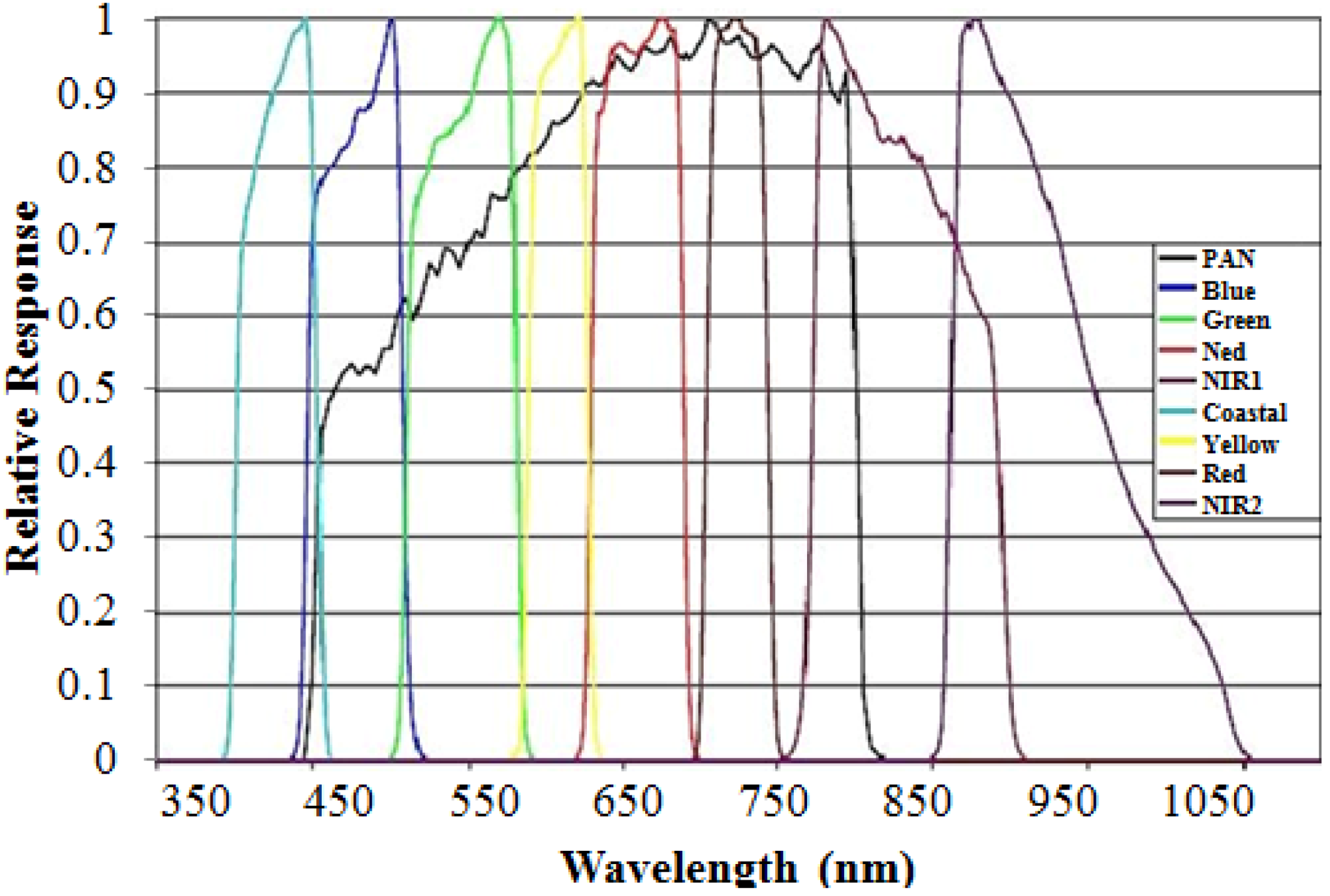
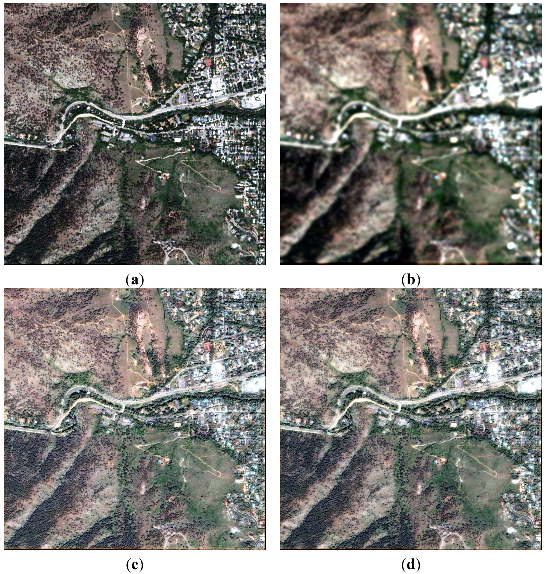
We conducted experiments using two datasets acquired by the QuickBird and WorldView-2 satellites. The selected QuickBird data, with 0.6-m Pan and 2.4-m MS images, consisted of a forest landscape bisected by a broad road near Boulder City, Colorado, U.S. (Figure 1). The MS image consisted of four bands, including R, G, B and NIR. The MS image was 600 × 600 pixels in size with a 2.4-m spatial resolution. The WorldView-2, which simultaneously collects Pan imagery at 0.46 m and MS imagery at 1.84 m, was the first commercial HR satellite to provide eight spectral sensors in the visible NIR range. Due to U.S. government licensing, the imagery information is made commercially available at 0.5 m and 2.0 m. In our dataset, the MS image was 800 × 800 pixels in size with a 2.0-m spatial resolution. We divided the eight MS bands into two groups for testing according to their bandwidth relationship with the Pan band (Figure 2). The first group contained bands 3 (green), 4 (yellow), 5 (red) and 6 (red edge), which were all covered by the Pan band wavelength. For the second group, we selected bands 1 (coastal), 2 (blue), 7 (NIR1) and 8 (NIR2), which were either not covered or not fully covered by the Pan band wavelength. The WorldView-2 scene subset, which contained many complex urban buildings and vegetation across San Francisco, was observed on 9 October 2011 (Figure 1). DigitalGlobe released the data through the 2012 IEEE GRSS Data Fusion Contest.

Figure 1. Color compositions of (a) the original QuickBird MS image (2.4 m) at 600 × 600 pixels combined from red, green and blue bands and (b) the original WorldView-2 MS image (2.0 m) at 800 × 800 pixels combined from green, red and red edge bands. The degraded Pan images for (c) QuickBird at 2.4 m and (d) WorldView-2 at 2.0 m.

Figure 1. Color compositions of (a) the original QuickBird MS image (2.4 m) at 600 × 600 pixels combined from red, green and blue bands and (b) the original WorldView-2 MS image (2.0 m) at 800 × 800 pixels combined from green, red and red edge bands. The degraded Pan images for (c) QuickBird at 2.4 m and (d) WorldView-2 at 2.0 m.

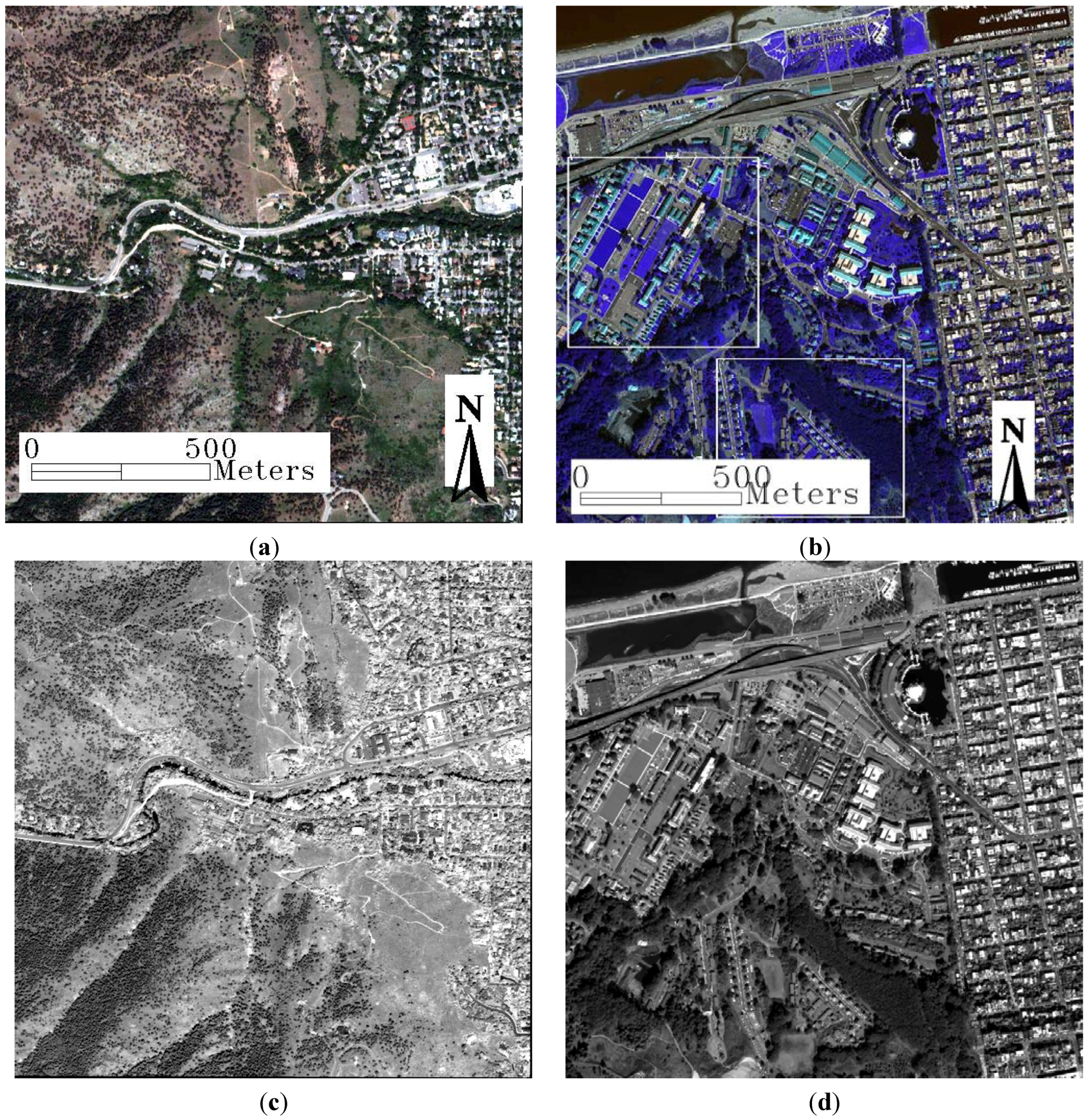
Figure 2. Relative spectral radiance response of the WorldView-2 instrument. The bandwidths are Coastal: 400–450 nm, Blue: 450–510 nm, Green: 510–580 nm, Yellow: 585–625 nm, Red: 630–690 nm, Red Edge: 705–745 nm, NIR1: 770–895 nm and NIR2: 860–1040 nm. (Image credit: Digital Globe.)

Figure 2. Relative spectral radiance response of the WorldView-2 instrument. The bandwidths are Coastal: 400–450 nm, Blue: 450–510 nm, Green: 510–580 nm, Yellow: 585–625 nm, Red: 630–690 nm, Red Edge: 705–745 nm, NIR1: 770–895 nm and NIR2: 860–1040 nm. (Image credit: Digital Globe.)

3.2. Validation Strategies

We conducted pan-sharpening at both reduced and full scales. At the reduced scale, we degraded the Pan and MS images by four before fusion so that we could use the original MS data as references for the fusion result evaluation. We applied a low-pass filter to the HR data, decimated the filtered images by two along both directions, reapplied the same filter and decimated the images again by two. We used 23-taps and ATW low-pass filters on the Pan and MS images, respectively [27,28] to match the MTF of the bands. At the full scale, we directly pansharpened the original MS images using the original Pan image and thus no MS reference images were used for the fusion results evaluation.

The consistency property of the Wald’s protocol, the synthesis property of the Wald’s protocol and Alparone’s protocol without reference were adopted as the validation strategies. To check the consistency property of the Wald’s protocol, we degraded all of the fused products to the original MS resolution by mimicking the sensor PSF [52]. We then evaluated the degraded fused MS product against the original reference MS images. This validation can be applied to both the reduced and full scale experiments. To check the synthesis property of the Wald’s protocol, we need the reference HR MS images and thus can only be applied to the reduced scale experiments. To check the Alparone’s protocol, we do not need the reference HR MS images and thus can be applied to the full scale experiments. Obviously, with reference available, the validation procedure of the consistency and synthesis properties of the Wald’s protocol is very accurate. However, the consistency property is just a necessary condition but not a sufficient condition to guarantee the fused image quality. And the synthesis property is founded on the hypothesis of invariance between scales, which is not always fulfilled in practice [51]. As such validation using Alparone’s protocol without reference is still necessary. Furthermore, a visual comparison is a mandatory step to appreciate the quality of the fused images.

If there are reference images in validation as in checking the consistency and synthesis properties of the Wald’s protocol, four quality indices can be adopted. (1) The first is the ERGAS index, from its French name “relative dimensionless global error in synthesis,” which calculates the amount of spectral distortion [84]. The best ERGAS value is zero; (2) The second is the Q4 index proposed by [85], which is an extension of the universal quality index (i.e., Q) suitable for four-band MS images. This index is sensitive to both correlation loss and spectral distortion between two MS images, and allows both spectral and spectral distortions to be combined in a unique parameter. The best value is one, with a range from zero to one. In our experiments, we calculated Q4 on 32 × 32 blocks; (3) The third is the spectral angle mapper (SAM), which calculates the angle between two spectral vectors to estimate the similarities between two different images. The best value is zero. (4) The last is signal to noise ratio (SNR, [86]) in decibel (dB). It is used to measure the ratio between information and noise of the fused image.

If there are no reference images in validation as in checking Alparone’s protocol, three following different quality indices can be adopted. (1) A spectral distortion index, D_λ, is derived from the difference of inter-band Q values calculated from the fused MS bands and from the original LR MS bands; (2) A spatial distortion index, D_S, is derived from the difference of inter-band Q values calculated between the fused MS bands and HR Pan band and between the original LR MS bands and the degraded Pan band; (3) QNR (i.e., Quality with No Reference) is a combination of the preceding spectral/spatial distortion index [87]. They all take values in [0, 1], with zero being the best value for D_λ and D_S, and one being the best value for QNR.

3.3. Experimental Results

Figure 3, Figure 4 and Figure 5 show the fusion results of different pansharpening methods for the QuickBird and WorldView-2 datasets at the reduced scale. The quantitative evaluation indices are reported in Table 2, Table 3, Table 4, Table 5, Table 6, Table 7, Table 8, Table 9, Table 10, Table 11, Table 12 and Table 13, which checked the synthesis property of the Wald’s protocol at the reduced scale (Table 2, Table 6 and Table 10), the consistency property of the Wald’s protocol at both the reduced and full scale (Table 3, Table 5, Table 7, Table 9, Table 11 and Table 13) and Alparone’s protocol without reference at the full scale (Table 4, Table 8 and Table 12).

Table 2. Quantitative comparison of the fusion results to check the synthesis property of the Wald’s protocol for the QuickBird dataset at the reduced scale, i.e., at 2.4 m. The best result in each row is displayed in bold, and the second best is displayed in italics. The shaded gray cells are for alternative group columns with different categories.

Category	No-Sharpening	CS		MRA-Local		MRA-Global
Method	EXP	GS	GS-S	ECB	ECB-S	M3, s = 0.5	M3-S	s = 0.75	s = 0.75, S	s = 0.9	s = 0.9, S
ERGAS	5.132	4.690	3.515	5.122	4.303	3.942	3.312	4.790	4.086	5.699	4.815
Q4	0.579	0.851	0.890	0.822	0.860	0.853	0.894	0.825	0.861	0.793	0.831
SAM (◦)	4.946	5.511	4.449	6.029	4.993	5.064	4.123	5.513	4.491	6.104	4.840
SNR	14.56	15.92	17.98	15.01	16.45	16.93	18.44	15.32	16.68	13.97	15.36

Table 2. Quantitative comparison of the fusion results to check the synthesis property of the Wald’s protocol for the QuickBird dataset at the reduced scale, i.e., at 2.4 m. The best result in each row is displayed in bold, and the second best is displayed in italics. The shaded gray cells are for alternative group columns with different categories.

Category	No-Sharpening	CS		MRA-Local		MRA-Global
Method	EXP	GS	GS-S	ECB	ECB-S	M3, s = 0.5	M3-S	s = 0.75	s = 0.75, S	s = 0.9	s = 0.9, S
ERGAS	5.132	4.690	3.515	5.122	4.303	3.942	3.312	4.790	4.086	5.699	4.815
Q4	0.579	0.851	0.890	0.822	0.860	0.853	0.894	0.825	0.861	0.793	0.831
SAM (◦)	4.946	5.511	4.449	6.029	4.993	5.064	4.123	5.513	4.491	6.104	4.840
SNR	14.56	15.92	17.98	15.01	16.45	16.93	18.44	15.32	16.68	13.97	15.36

Table 3. Quantitative comparison of the fusion results after degrading the images into the LR resolution, i.e., at 9.6 m, to check the consistency property of the Wald’s protocol for the QuickBird dataset at the reduced scale.

Method	EXP	GS	GS-S	ECB	ECB-S	M3	M3-S	s = 0.75	s = 0.75, S	s = 0.9	s = 0.9, S
ERGAS	1.166	1.881	0.402	1.033	0.804	0.919	0.357	1.016	0.539	1.149	0.701
Q4	0.983	0.986	0.999	0.990	0.999	0.991	0.999	0.989	0.999	0.986	0.998
SAM (◦)	1.098	1.330	0.235	1.140	0.282	1.118	0.214	1.148	0.256	1.188	0.314
SNR	27.26	23.93	36.79	28.65	31.89	29.46	37.50	28.61	34.21	27.65	32.23

Table 3. Quantitative comparison of the fusion results after degrading the images into the LR resolution, i.e., at 9.6 m, to check the consistency property of the Wald’s protocol for the QuickBird dataset at the reduced scale.

Method	EXP	GS	GS-S	ECB	ECB-S	M3	M3-S	s = 0.75	s = 0.75, S	s = 0.9	s = 0.9, S
ERGAS	1.166	1.881	0.402	1.033	0.804	0.919	0.357	1.016	0.539	1.149	0.701
Q4	0.983	0.986	0.999	0.990	0.999	0.991	0.999	0.989	0.999	0.986	0.998
SAM (◦)	1.098	1.330	0.235	1.140	0.282	1.118	0.214	1.148	0.256	1.188	0.314
SNR	27.26	23.93	36.79	28.65	31.89	29.46	37.50	28.61	34.21	27.65	32.23

Table 4. Quantitative comparison of the fusion results to check Alparone’s protocol for the QuickBird dataset at full scale, i.e., at 0.6 m. Time is measured in minutes. The font face indicators are identical to those in Table 2.

Method	EXP	GS	GS-S	ECB	ECB-S	M3	M3-S	s = 0.75	s = 0.75, S	s = 0.9	s = 0.9, S
Dλ	0.037	0.117	0.034	0.081	0.057	0.070	0.030	0.119	0.055	0.149	0.078
Ds	0.193	0.174	0.023	0.045	0.021	0.070	0.040	0.139	0.024	0.162	0.042
QNR	0.777	0.729	0.944	0.878	0.922	0.864	0.931	0.758	0.922	0.713	0.883
Time	0.02	0.28	6.30	3.10	9.12	0.27	6.29	0.29	6.42	0.28	6.44

Table 4. Quantitative comparison of the fusion results to check Alparone’s protocol for the QuickBird dataset at full scale, i.e., at 0.6 m. Time is measured in minutes. The font face indicators are identical to those in Table 2.

Method	EXP	GS	GS-S	ECB	ECB-S	M3	M3-S	s = 0.75	s = 0.75, S	s = 0.9	s = 0.9, S
Dλ	0.037	0.117	0.034	0.081	0.057	0.070	0.030	0.119	0.055	0.149	0.078
Ds	0.193	0.174	0.023	0.045	0.021	0.070	0.040	0.139	0.024	0.162	0.042
QNR	0.777	0.729	0.944	0.878	0.922	0.864	0.931	0.758	0.922	0.713	0.883
Time	0.02	0.28	6.30	3.10	9.12	0.27	6.29	0.29	6.42	0.28	6.44

Table 5. Quantitative comparison of the fusion results after degrading the images into the LR resolution, i.e., at 2.4 m, to check the consistency property of the Wald’s protocol for the QuickBird dataset at full scale.

Method	EXP	GS	GS-S	ECB	ECB-S	M3	M3-S	s = 0.75	s = 0.75, S	s = 0.9	s = 0.9, S
ERGAS	0.815	2.490	0.303	1.170	0.620	0.845	0.232	1.232	0.349	1.552	0.429
Q4	0.989	0.966	0.998	0.983	0.992	0.988	0.999	0.977	0.998	0.967	0.996
SAM (◦)	0.880	1.537	0.375	1.036	0.652	0.867	0.310	0.986	0.339	1.112	0.365

Table 5. Quantitative comparison of the fusion results after degrading the images into the LR resolution, i.e., at 2.4 m, to check the consistency property of the Wald’s protocol for the QuickBird dataset at full scale.

Method	EXP	GS	GS-S	ECB	ECB-S	M3	M3-S	s = 0.75	s = 0.75, S	s = 0.9	s = 0.9, S
ERGAS	0.815	2.490	0.303	1.170	0.620	0.845	0.232	1.232	0.349	1.552	0.429
Q4	0.989	0.966	0.998	0.983	0.992	0.988	0.999	0.977	0.998	0.967	0.996
SAM (◦)	0.880	1.537	0.375	1.036	0.652	0.867	0.310	0.986	0.339	1.112	0.365

Table 6. Quantitative comparison of the fusion results to check the synthesis property of the Wald’s protocol for the WorldView-2 group 1 dataset at the reduced scale, i.e., at 2.0 m. The font face indicators are identical to those in Table 2.

Method	EXP	GS	GS-S	ECB	ECB-S	M3	M3-S	s = 0.75	s = 0.75, S	s = 0.9	s = 0.9, S
ERGAS	9.340	5.573	4.368	4.093	3.846	4.225	3.939	4.033	3.728	3.994	3.671
Q4	0.542	0.875	0.906	0.923	0.931	0.912	0.924	0.923	0.933	0.926	0.936
SAM (◦)	6.106	6.184	5.400	5.820	5.290	6.019	5.317	5.950	5.282	5.935	5.275
SNR	9.92	14.92	16.52	17.13	17.64	16.83	17.42	17.24	17.90	17.33	18.03

Table 6. Quantitative comparison of the fusion results to check the synthesis property of the Wald’s protocol for the WorldView-2 group 1 dataset at the reduced scale, i.e., at 2.0 m. The font face indicators are identical to those in Table 2.

Method	EXP	GS	GS-S	ECB	ECB-S	M3	M3-S	s = 0.75	s = 0.75, S	s = 0.9	s = 0.9, S
ERGAS	9.340	5.573	4.368	4.093	3.846	4.225	3.939	4.033	3.728	3.994	3.671
Q4	0.542	0.875	0.906	0.923	0.931	0.912	0.924	0.923	0.933	0.926	0.936
SAM (◦)	6.106	6.184	5.400	5.820	5.290	6.019	5.317	5.950	5.282	5.935	5.275
SNR	9.92	14.92	16.52	17.13	17.64	16.83	17.42	17.24	17.90	17.33	18.03

Table 7. Quantitative comparison of the fusion results after degrading the images into the LR resolution, i.e., at 8.0 m, to check the consistency property of the Wald’s protocol for the WorldView-2 group 1 dataset at the reduced scale.

Method	EXP	GS	GS-S	ECB	ECB-S	M3	M3-S	s = 0.75	s = 0.75, S	s = 0.9	s = 0.9, S
ERGAS	1.908	2.439	0.168	0.646	0.190	0.644	0.136	0.663	0.139	0.685	0.143
Q4	0.977	0.982	1.000	0.997	1.000	0.997	1.000	0.997	1.000	0.997	1.000
SAM (◦)	1.154	1.333	0.205	1.009	0.284	1.070	0.183	1.064	0.183	1.067	0.184
SNR	23.13	21.65	44.21	32.75	43.16	32.73	46.02	32.50	45.79	32.23	45.55

Table 7. Quantitative comparison of the fusion results after degrading the images into the LR resolution, i.e., at 8.0 m, to check the consistency property of the Wald’s protocol for the WorldView-2 group 1 dataset at the reduced scale.

Method	EXP	GS	GS-S	ECB	ECB-S	M3	M3-S	s = 0.75	s = 0.75, S	s = 0.9	s = 0.9, S
ERGAS	1.908	2.439	0.168	0.646	0.190	0.644	0.136	0.663	0.139	0.685	0.143
Q4	0.977	0.982	1.000	0.997	1.000	0.997	1.000	0.997	1.000	0.997	1.000
SAM (◦)	1.154	1.333	0.205	1.009	0.284	1.070	0.183	1.064	0.183	1.067	0.184
SNR	23.13	21.65	44.21	32.75	43.16	32.73	46.02	32.50	45.79	32.23	45.55

Table 8. Quantitative comparison of the fusion results to check Alparone’s protocol for the WorldView-2 group 1 dataset at full scale, i.e., at 0.5 m. Time is measured in minutes. The font face indicators are identical to those in Table 2.

Method	EXP	GS	GS-S	ECB	ECB-S	M3	M3-S	s = 0.75	s = 0.75, S	s = 0.9	s = 0.9, S
Dλ	0.046	0.013	0.015	0.021	0.012	0.030	0.013	0.035	0.018	0.036	0.020
Ds	0.197	0.023	0.024	0.010	0.023	0.015	0.019	0.018	0.009	0.019	0.007
QNR	0.766	0.964	0.962	0.969	0.965	0.955	0.969	0.948	0.974	0.945	0.974
Time	0.03	0.50	11.20	5.64	16.25	0.48	11.22	0.49	11.21	0.49	11.31

Table 8. Quantitative comparison of the fusion results to check Alparone’s protocol for the WorldView-2 group 1 dataset at full scale, i.e., at 0.5 m. Time is measured in minutes. The font face indicators are identical to those in Table 2.

Method	EXP	GS	GS-S	ECB	ECB-S	M3	M3-S	s = 0.75	s = 0.75, S	s = 0.9	s = 0.9, S
Dλ	0.046	0.013	0.015	0.021	0.012	0.030	0.013	0.035	0.018	0.036	0.020
Ds	0.197	0.023	0.024	0.010	0.023	0.015	0.019	0.018	0.009	0.019	0.007
QNR	0.766	0.964	0.962	0.969	0.965	0.955	0.969	0.948	0.974	0.945	0.974
Time	0.03	0.50	11.20	5.64	16.25	0.48	11.22	0.49	11.21	0.49	11.31

Table 9. Quantitative comparison of the fusion results after degrading the images into the LR resolution, i.e., at 2.0 m, to check the consistency property of the Wald’s protocol for the WorldView-2 group 1 dataset at full scale.

Method	EXP	GS	GS-S	ECB	ECB-S	M3	M3-S	s = 0.75	s = 0.75, S	s = 0.9	s = 0.9, S
ERGAS	1.453	2.894	0.732	1.191	0.934	1.104	0.642	1.191	0.776	1.230	0.838
Q4	0.990	0.965	0.997	0.993	0.996	0.994	0.998	0.993	0.997	0.993	0.997
SAM (◦)	0.927	1.433	0.420	0.860	0.523	0.925	0.353	0.931	0.417	0.936	0.448

Table 9. Quantitative comparison of the fusion results after degrading the images into the LR resolution, i.e., at 2.0 m, to check the consistency property of the Wald’s protocol for the WorldView-2 group 1 dataset at full scale.

Method	EXP	GS	GS-S	ECB	ECB-S	M3	M3-S	s = 0.75	s = 0.75, S	s = 0.9	s = 0.9, S
ERGAS	1.453	2.894	0.732	1.191	0.934	1.104	0.642	1.191	0.776	1.230	0.838
Q4	0.990	0.965	0.997	0.993	0.996	0.994	0.998	0.993	0.997	0.993	0.997
SAM (◦)	0.927	1.433	0.420	0.860	0.523	0.925	0.353	0.931	0.417	0.936	0.448

Table 10. Quantitative comparison of the fusion results to check the synthesis property of the Wald’s protocol for the WorldView-2 group 2 dataset at the reduced scale, i.e., at 2.0 m. The font face indicators are identical to those in Table 2.

Method	EXP	GS	GS-S	ECB	ECB-S	M3	M3-S	s = 0.75	s = 0.75, S	s = 0.9	s = 0.9, S
ERGAS	8.098	11.01	5.404	6.289	5.474	6.129	5.423	5.988	5.130	7.206	5.676
Q4	0.516	0.705	0.849	0.803	0.845	0.751	0.820	0.810	0.858	0.801	0.852
SAM (◦)	8.769	9.850	6.581	7.383	6.600	7.729	6.735	7.206	6.383	8.428	6.934
SNR	12.48	12.80	16.04	16.18	16.98	16.11	16.93	16.36	17.36	15.50	16.88

Table 10. Quantitative comparison of the fusion results to check the synthesis property of the Wald’s protocol for the WorldView-2 group 2 dataset at the reduced scale, i.e., at 2.0 m. The font face indicators are identical to those in Table 2.

Method	EXP	GS	GS-S	ECB	ECB-S	M3	M3-S	s = 0.75	s = 0.75, S	s = 0.9	s = 0.9, S
ERGAS	8.098	11.01	5.404	6.289	5.474	6.129	5.423	5.988	5.130	7.206	5.676
Q4	0.516	0.705	0.849	0.803	0.845	0.751	0.820	0.810	0.858	0.801	0.852
SAM (◦)	8.769	9.850	6.581	7.383	6.600	7.729	6.735	7.206	6.383	8.428	6.934
SNR	12.48	12.80	16.04	16.18	16.98	16.11	16.93	16.36	17.36	15.50	16.88

Table 11. Quantitative comparison of the fusion results after degrading the images into the LR resolution, i.e., at 8.0 m, to check the consistency property of the Wald’s protocol for the WorldView-2 group 2 dataset at the reduced scale.

Method	EXP	GS	GS-S	ECB	ECB-S	M3	M3-S	s = 0.75	s = 0.75, S	s = 0.9	s = 0.9, S
ERGAS	1.632	7.631	0.353	1.368	0.412	1.202	0.220	1.333	0.262	1.793	0.480
Q4	0.974	0.826	0.999	0.985	0.999	0.987	1.000	0.986	0.999	0.976	0.998
SAM (◦)	1.726	6.976	0.388	1.587	0.487	1.484	0.263	1.547	0.283	1.989	0.480
SNR	25.97	17.64	40.60	30.16	38.13	30.65	42.69	29.95	41.36	28.40	38.15

Table 11. Quantitative comparison of the fusion results after degrading the images into the LR resolution, i.e., at 8.0 m, to check the consistency property of the Wald’s protocol for the WorldView-2 group 2 dataset at the reduced scale.

Method	EXP	GS	GS-S	ECB	ECB-S	M3	M3-S	s = 0.75	s = 0.75, S	s = 0.9	s = 0.9, S
ERGAS	1.632	7.631	0.353	1.368	0.412	1.202	0.220	1.333	0.262	1.793	0.480
Q4	0.974	0.826	0.999	0.985	0.999	0.987	1.000	0.986	0.999	0.976	0.998
SAM (◦)	1.726	6.976	0.388	1.587	0.487	1.484	0.263	1.547	0.283	1.989	0.480
SNR	25.97	17.64	40.60	30.16	38.13	30.65	42.69	29.95	41.36	28.40	38.15

Table 12. Quantitative comparison of the fusion results to check Alparone’s protocol for the WorldView-2 group 2 dataset at full scale, i.e., at 0.5 m. Time is measured in minutes. The font face indicators are identical to those in Table 2.

Method	EXP	GS	GS-S	ECB	ECB-S	M3	M3-S	s = 0.75	s = 0.75, S	s = 0.9	s = 0.9, S
Dλ	0.024	0.065	0.023	0.060	0.044	0.072	0.045	0.078	0.050	0.072	0.048
Ds	0.151	0.217	0.077	0.049	0.042	0.039	0.026	0.068	0.021	0.067	0.013
QNR	0.828	0.732	0.902	0.894	0.915	0.892	0.931	0.860	0.930	0.866	0.939
Time	0.03	0.50	11.29	5.67	16.32	0.52	11.15	0.49	11.10	0.50	11.26

Table 12. Quantitative comparison of the fusion results to check Alparone’s protocol for the WorldView-2 group 2 dataset at full scale, i.e., at 0.5 m. Time is measured in minutes. The font face indicators are identical to those in Table 2.

Method	EXP	GS	GS-S	ECB	ECB-S	M3	M3-S	s = 0.75	s = 0.75, S	s = 0.9	s = 0.9, S
Dλ	0.024	0.065	0.023	0.060	0.044	0.072	0.045	0.078	0.050	0.072	0.048
Ds	0.151	0.217	0.077	0.049	0.042	0.039	0.026	0.068	0.021	0.067	0.013
QNR	0.828	0.732	0.902	0.894	0.915	0.892	0.931	0.860	0.930	0.866	0.939
Time	0.03	0.50	11.29	5.67	16.32	0.52	11.15	0.49	11.10	0.50	11.26

Table 13. Quantitative comparison of the fusion results after degrading the images into the LR resolution, i.e., at 2.0 m, to check the consistency property of the Wald’s protocol for the WorldView-2 group 2 dataset at full scale.

Method	EXP	GS	GS-S	ECB	ECB-S	M3	M3-S	s = 0.75	s = 0.75, S	s = 0.9	s = 0.9, S
ERGAS	1.286	8.393	0.375	1.369	0.812	1.087	0.267	1.345	0.371	1.719	0.477
Q4	0.989	0.804	0.999	0.988	0.995	0.992	1.000	0.989	0.999	0.982	0.999
SAM (◦)	1.365	6.644	0.381	1.364	0.738	1.202	0.217	1.336	0.271	1.612	0.348

Table 13. Quantitative comparison of the fusion results after degrading the images into the LR resolution, i.e., at 2.0 m, to check the consistency property of the Wald’s protocol for the WorldView-2 group 2 dataset at full scale.

Method	EXP	GS	GS-S	ECB	ECB-S	M3	M3-S	s = 0.75	s = 0.75, S	s = 0.9	s = 0.9, S
ERGAS	1.286	8.393	0.375	1.369	0.812	1.087	0.267	1.345	0.371	1.719	0.477
Q4	0.989	0.804	0.999	0.988	0.995	0.992	1.000	0.989	0.999	0.982	0.999
SAM (◦)	1.365	6.644	0.381	1.364	0.738	1.202	0.217	1.336	0.271	1.612	0.348

3.3.1. Degree of Spatial Enhancement

The GLP-based methods (e.g., the GLP-M3 method) could exhibit better spatial enhancement than the GS method when the s value was adjusted properly. In all of these figures, when s is set to be larger than 0.75, the spatial enhancement of the MRA methods is larger than that of the GS method (Figure 3, Figure 4 and Figure 5).

3.3.2. Are the Up-Sampled Images Spectrally Consistent?

None of the up-sampled images found to be strictly spectrally consistent from both the quantitative measurements and visual comparisons. The consistency quantitative matrices of the up-sampled images were shown in the first columns of Table 3, Table 5, Table 7, Table 9, Table 11 and Table 13 (3, 7 and 11 for the reduced scale, and 5, 9 and 13 for the full scale). The ERGAS values are around 1, which is not close to 0. In Figure 3, Figure 4 and Figure 5, we can also see that that the up-sampled images have larger spectral distortions than the MRA fused images as opposed to the reference images, e.g., the roofs in Figure 3 and Figure 4 and the vegetation in Figure 5.

None of the MRA methods actually satisfied the spectral consistency property (Table 3, Table 5, Table 7, Table 9, Table 11 and Table 13). However, the spectral consistency performance of the GLP-based methods was always better than that of the GS method even when the s value increased from 0.5 to 0.75 and 0.9 for the M3 method to gain more spatial enhancement. This indicated that although the GLP-based methods were not spectrally consistent by design, their spectral inconsistency was not as obvious as that of the GS method. That is why so many studies have stated that GLP-based methods perform better in terms of spectral preservation.

3.3.3. Spectral Preservation is Complementary with Spatial Injection

All of the fused images at both the reduced and full scales were almost perfectly spectrally consistent with the LR MS images by adding the spectral consistency constraint (Table 3, Table 5, Table 7, Table 9, Table 11 and Table 13). They all had Q4 values close to 1, big SNR values, and very small ERGAS and SAM values when checking the consistency property at their LR resolutions [52]. The fused products under the spectral consistency constraint also had better quantitative evaluation indices when checking the synthesis property (Table 2, Table 6 and Table 10) and checking Alparone’s protocol (Table 4, Table 8 and Table 12). This improvement was obvious given the respective one-unit decrease in ERGAS and SAM values for the GLP-based methods (Table 2, Table 6 and Table 10). The improvement was even more obvious for the GS method, which made GS-S the second best performance for the QuickBird and WorldView-2 group 2 datasets. The performance increases were also obvious visually. For example, the tone in Figure 3d (GS-S) is closer to the observed reference scene than that in Figure 3c (GS). However, there is a case for the WorldView-2 group 1 dataset (Table 8) that the ECB method with spectral consistency constraint showed no improvement in terms of QNR metric. This is possibly because that the QNR at the full scale is not as reliable as the other metrics used at the reduced scale [88] or because that the spatial independence assumptions is violated in the HR dataset.

Furthermore, we found only a negligible decrease in spatial enhancement after making the fused products spectrally consistent (Figure 3, Figure 4 and Figure 5). This indicated that spectral consistency, which is quite different from spectral preservation to the up-sampled MS images, is complementary with spatial enhancement rather than competitive. For example, comparing the GS-S and GS methods, the sharpness was only slightly weakened (Figure 3, Figure 4 and Figure 5e and f). Moreover the GS-S method performed very closely to the M3-S method, which indicated that the proposed spectral consistency model was quite effective for making up for the spectral distortion caused by the fusion method.

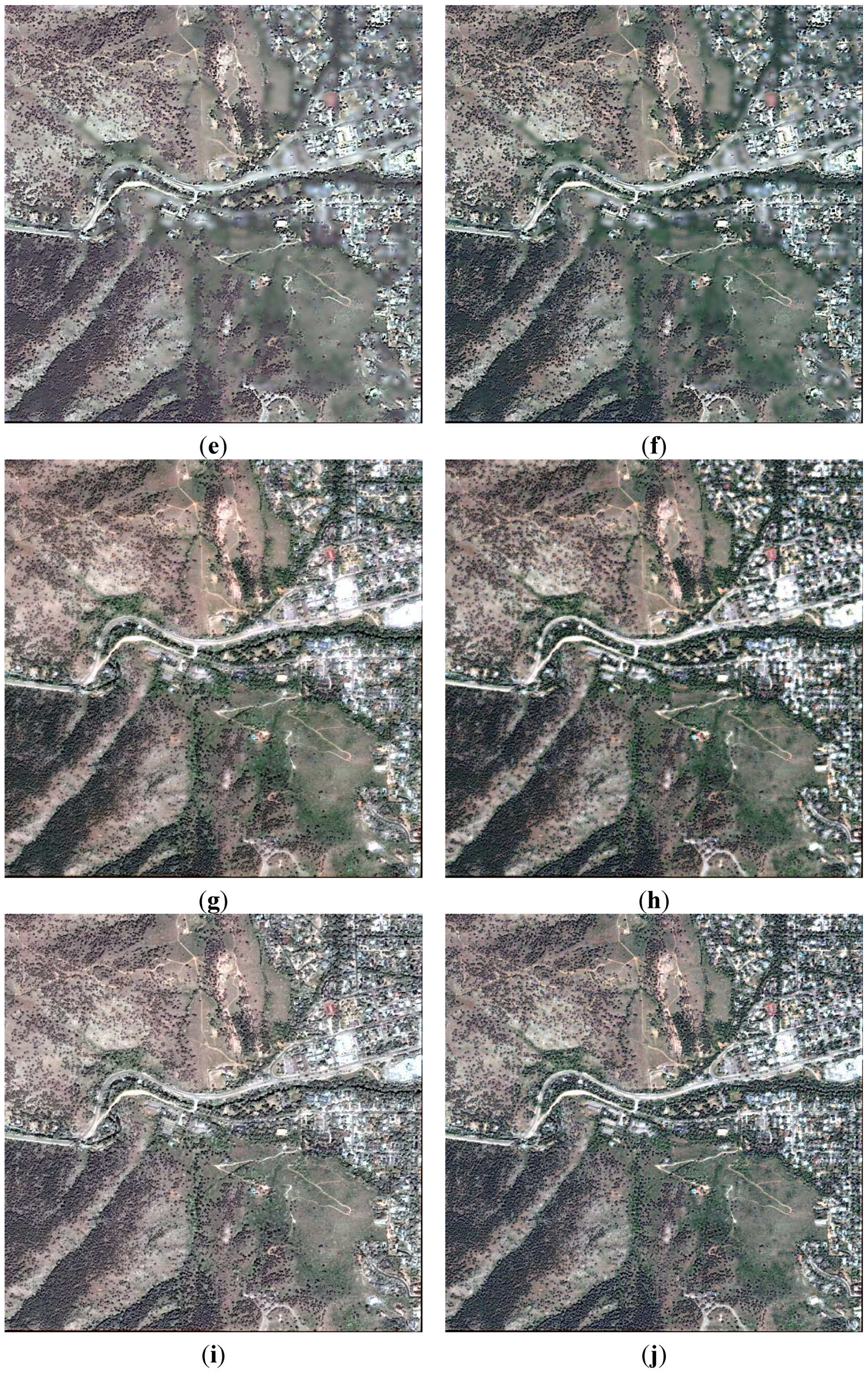
Figure 3. True color display of the fused results from different strategies for the QuickBird dataset at the reduced scale. (a): Observed at a 2.4-m spatial resolution; (b): EXP; (c): GS; (d): GS-spectrally consistent; (e): GLP-ECB; (f): GLP-ECB-spectrally consistent; (g): GLP-M3; (h): GLP-M3-spectrally consistent; (i): GLP with s = 0.75; (j): Spectrally consistent GLP with s = 0.75.

Figure 3. True color display of the fused results from different strategies for the QuickBird dataset at the reduced scale. (a): Observed at a 2.4-m spatial resolution; (b): EXP; (c): GS; (d): GS-spectrally consistent; (e): GLP-ECB; (f): GLP-ECB-spectrally consistent; (g): GLP-M3; (h): GLP-M3-spectrally consistent; (i): GLP with s = 0.75; (j): Spectrally consistent GLP with s = 0.75.

Figure 4. A subset, marked in the left white box in Figure 1, of different fusion results at the reduced scale of the WorldView-2 group 1 dataset. Bands 3, 5 and 6 are combined for RGB display. (a): Observed at a 2.0-m spatial resolution; (b): EXP; (c): GS; (d): GS-spectrally consistent; (e): GLP-ECB; (f): GLP-ECB-spatially consistent; (g): GLP-M3; (h): GLP-M3-spectrally consistent;(i): GLP with s = 0.75; (j): Spectrally consistent GLP with s = 0.75.

Figure 4. A subset, marked in the left white box in Figure 1, of different fusion results at the reduced scale of the WorldView-2 group 1 dataset. Bands 3, 5 and 6 are combined for RGB display. (a): Observed at a 2.0-m spatial resolution; (b): EXP; (c): GS; (d): GS-spectrally consistent; (e): GLP-ECB; (f): GLP-ECB-spatially consistent; (g): GLP-M3; (h): GLP-M3-spectrally consistent;(i): GLP with s = 0.75; (j): Spectrally consistent GLP with s = 0.75.

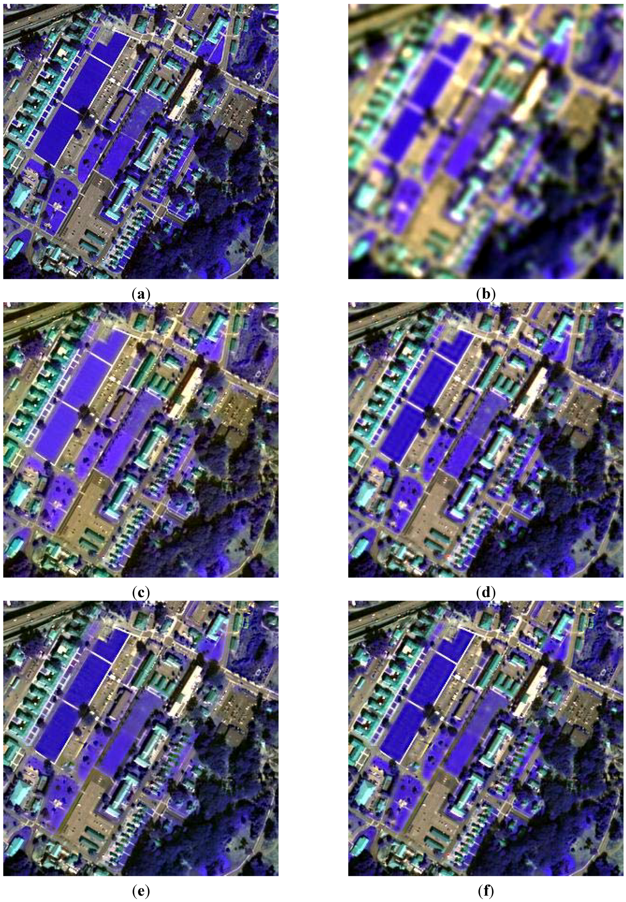
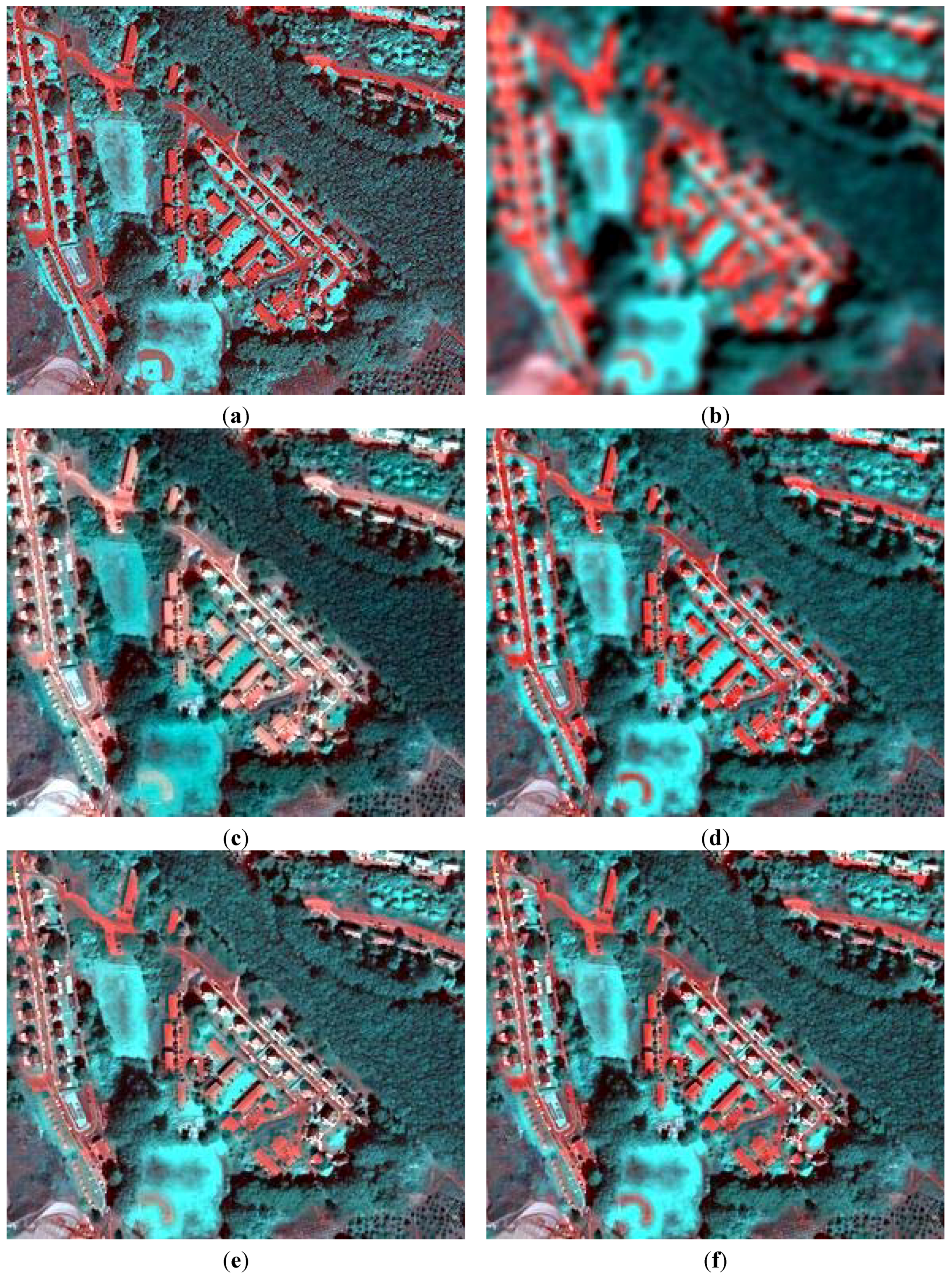
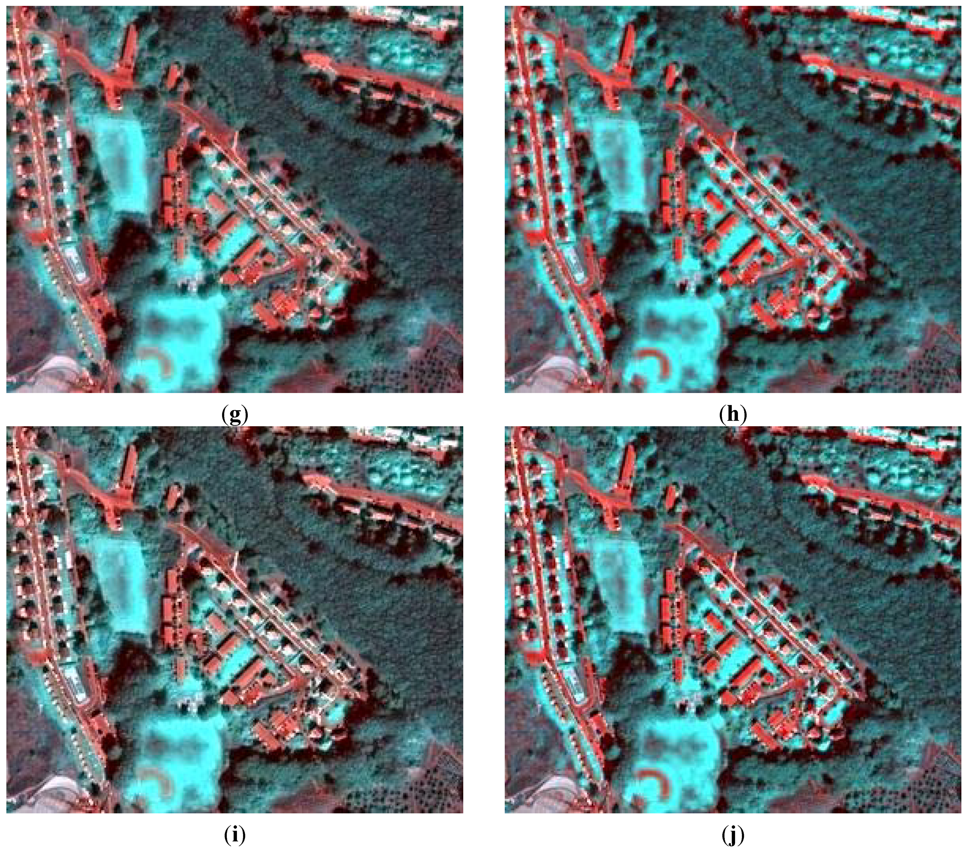
Figure 5. A subset, marked in the right white box in Figure 1, of different fusion results at the reduced scale of the WorldView-2 group 2 dataset. Bands 1, 7 and 8 are combined for RGB display. (a): Observed at a 2.0-m spatial resolution; (b): EXP; (c): GS; (d): GS-spectrally consistent; (e): GLP-ECB; (f): GLP-ECB-spatially consistent; (g): GLP-M3; (h): GLP-M3-spectrally consistent;(i): GLP with s = 0.75; (j): Spectrally consistent GLP with s = 0.75.

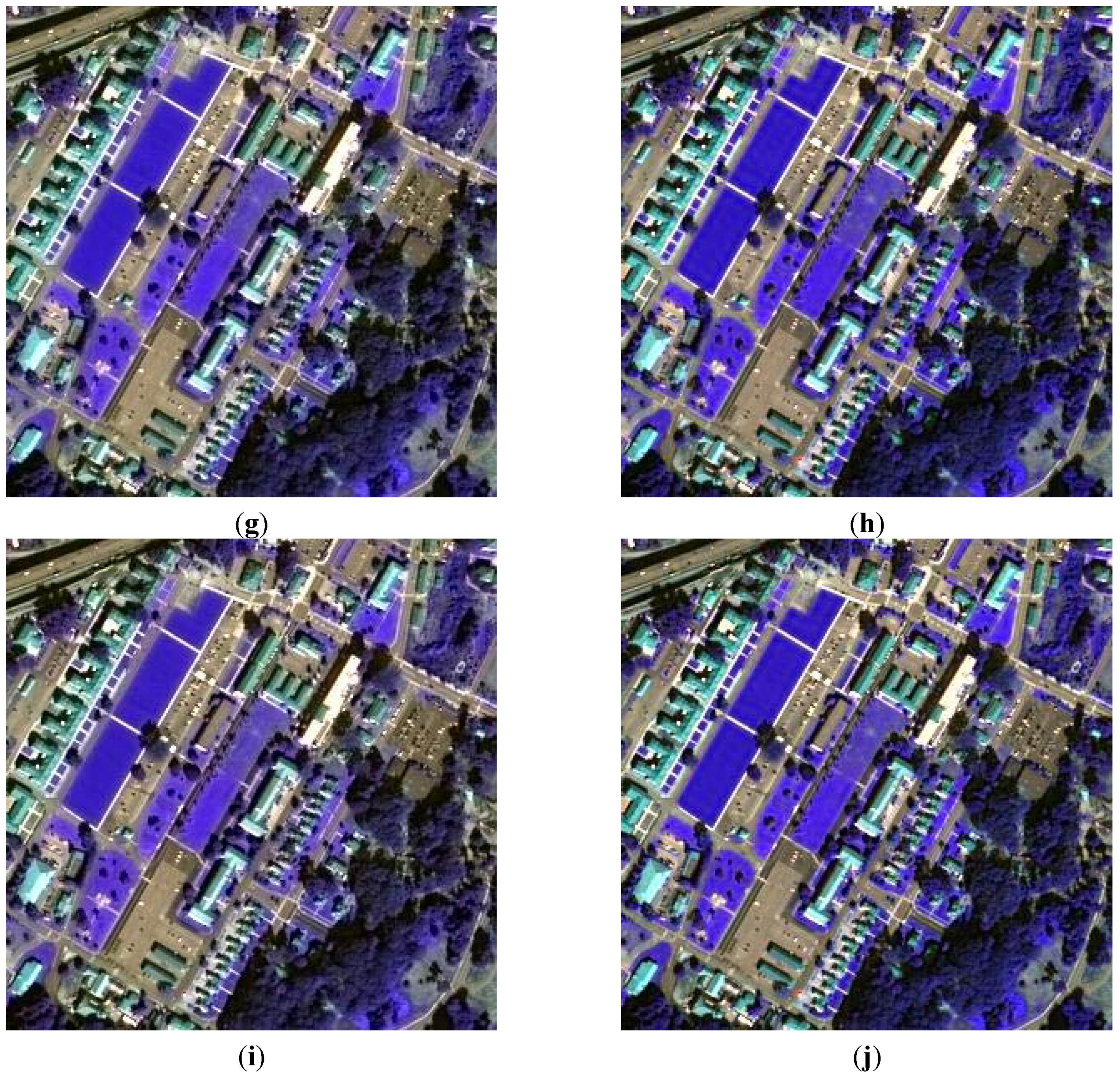
Figure 5. A subset, marked in the right white box in Figure 1, of different fusion results at the reduced scale of the WorldView-2 group 2 dataset. Bands 1, 7 and 8 are combined for RGB display. (a): Observed at a 2.0-m spatial resolution; (b): EXP; (c): GS; (d): GS-spectrally consistent; (e): GLP-ECB; (f): GLP-ECB-spatially consistent; (g): GLP-M3; (h): GLP-M3-spectrally consistent;(i): GLP with s = 0.75; (j): Spectrally consistent GLP with s = 0.75.

3.4. Discussions

The Bayesian perspective of the pansharpening methods can be supported by the GS performance dependence of the linear fitness of Equation (5) in our experimental results, i.e., the Pan approximation by the linear MS combination. As basic assumption of the GS method is the perfect linear relationship between the Pan band and MS bands, its performance may be largely affected by the fitness of this linear relationship. As shown in Table 14, the residual variance of the linear regression in Equations (5) and (18) for the WorldView-2 group 2 dataset is much larger (indicating worse representation of Equation 5) than that for the QuickBird and WorldView-2 group 1 datasets. Thus the GS method performed much worse for the WorldView-2 group 2 dataset than the other two datasets. Researchers have tried to make the regression residual as small as possible, such as via histogram matching in the original CS methods and via injecting spatial details into the linear combination results y in the combined CS/MRA method [34].

Table 14. The variance of the regression residual σ_e in Equation (18), the modulation coefficient ω^q in Equation (19) for the GS method and the weight parameter s^q in Equation (29) averaged over the image for the ECB method for the reduced scale experiments. Their average values over all the four bands are shown in the last column.

Band (q)		1	2	3	4	Average
QuickBird σe = 429	ωq: GS	0.589	1.086	0.940	1.384	1.00
	sq: ECB	0.565	0.536	0.575	0.715	0.597
WorldView-2, group 1 σe = 154	ω q: GS	0.948	1.183	0.849	1.020	1.00
	sq: ECB	0.621	0.595	0.583	0.655	0.613
WorldView-2, group 2 σe = 4558	ωq: GS	0.237	0.318	1.806	1.639	1.00
	sq: ECB	0.662	0.649	0.689	0.705	0.676

Table 14. The variance of the regression residual σ_e in Equation (18), the modulation coefficient ω^q in Equation (19) for the GS method and the weight parameter s^q in Equation (29) averaged over the image for the ECB method for the reduced scale experiments. Their average values over all the four bands are shown in the last column.

Band (q)		1	2	3	4	Average
QuickBird σe = 429	ωq: GS	0.589	1.086	0.940	1.384	1.00
	sq: ECB	0.565	0.536	0.575	0.715	0.597
WorldView-2, group 1 σe = 154	ω q: GS	0.948	1.183	0.849	1.020	1.00
	sq: ECB	0.621	0.595	0.583	0.655	0.613
WorldView-2, group 2 σe = 4558	ωq: GS	0.237	0.318	1.806	1.639	1.00
	sq: ECB	0.662	0.649	0.689	0.705	0.676

The Bayesian perspective of the pansharpening methods can also be supported by confirming the relationship between regression and modulation coefficients of the CS methods (i.e., Equation (20)). For the GS method, because the regression coefficient in Equation (18), β^q, equals 1/4, the average modulation coefficient (ω^q) value shown in Table 14 is actually Ʃβ^qω^q. They are all equal to 1, which satisfies Equation (20).

The s value is important as it controls the amount of modulation coefficient and thus the spatial enhancement degree. Theoretically setting s = 0.5 would get the best results as there is no prior information on the priority between the linear correlation assumption and the Gaussian distribution assumption. Thus when setting s = 0.5 the modulation coefficients were automatically and precisely controlled by the variance and covariance values in Equation (28). However, we could not estimate the variance and covariance properly due to the scale effect [18,87]. As such, the best s value should also compensate the scale effect which is hard to predict [51] and thus requires further research. For example, in our experiments, the best s value was not 0.5. Increasing s from 0.5 to 0.75, i.e., from M3 (s = 0. 5) and ECB (s ≈ 0. 6) to M3 with s = 0.75, resulted in some increase in the algorithm performance for all of the WorldView-2 datasets (The s values for the ECB method were spatially adaptive, with averages around 0.6, as shown in Table 14.)

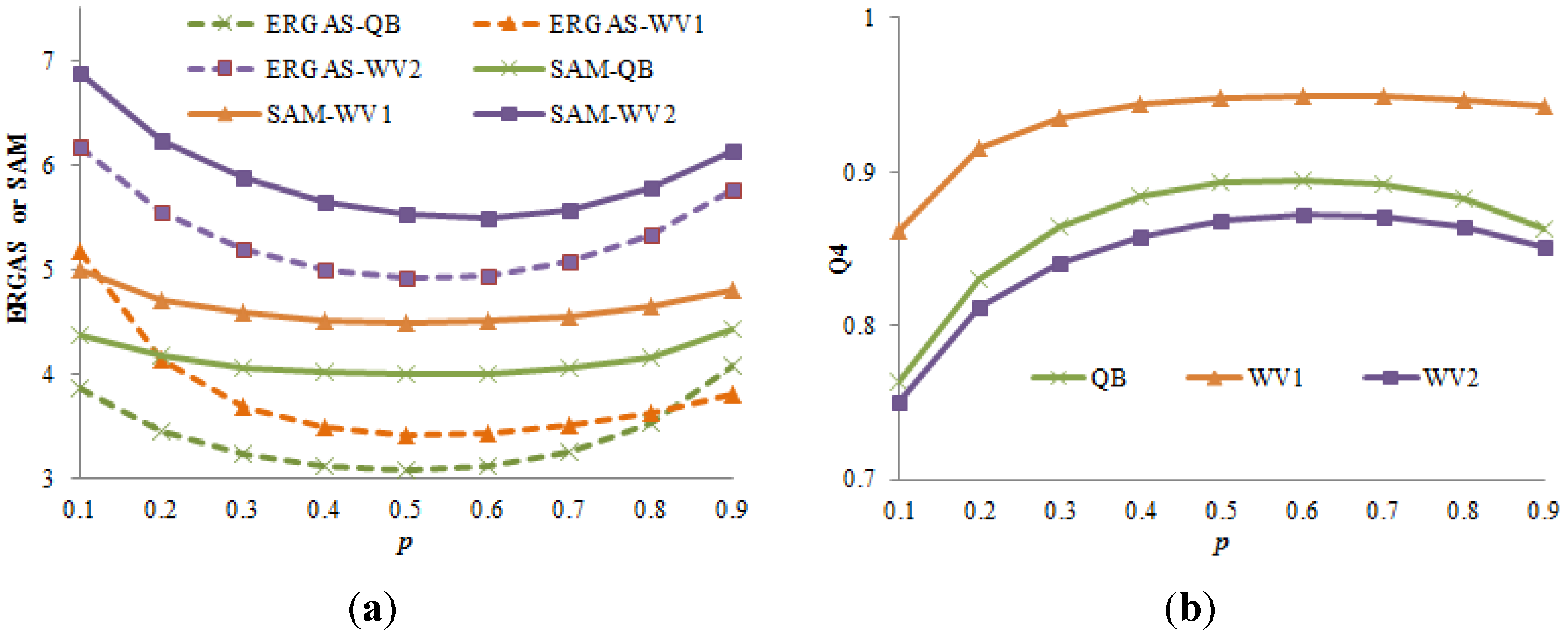
The Bayesian perspective of the pansharpening methods can also be supported by that experimentally the best s value is 0.5 when there is no scale effect in calculating variance and covariance. Figure 6 shows ERGAS, SAM and Q4 as functions of the s value in the GLP-based methods for the three datasets at the reduced scale. The coefficients were calculated based on the HR images to avoid the scale effect, which was not available in practice. Without exception, the best ERGAS, SAM and Q4 values were achieved by setting s = 0.5.

Figure 6. ERGAS, SAM (a) and Q4 (b) as functions of the s value in the GLP-based methods for all three datasets, including WorldView-2 (WV) and QuickBird (QB).

Figure 6. ERGAS, SAM (a) and Q4 (b) as functions of the s value in the GLP-based methods for all three datasets, including WorldView-2 (WV) and QuickBird (QB).

3.5. Computational Complexity

The last rows of Table 4, Table 8 and Table 12 show the computational times of each algorithm in the full scale experiments. We used an Intel^® Dual-Core™ i5 CPU with installed memory of 4.00 GB and a 32-bit Windows 7 operating system as the computer platform in the experiment. All of the codes were written in Matlab language.

The efficiency of the conjugate gradient search to guarantee the spectral consistency was acceptable in the computing environment for an LR MS image around 800 × 800 pixels in size. And it can be improved using recently developed parallel computing paradigm [89]. The algorithm efficiency was proportional to the product of the LR MS pixel number and the spectral band number (i.e., M × Q). This means that when the study area was increased, the computation time increased linearly along with the number of pixels. Compared with the ECB method, the main computational time of the ECB-S method was spent on the conjugate gradient search, as they required the same amount of time to calculate the modulation coefficients. Most of the time spent by the algorithms with the spectral consistency constraint was spent on the conjugate gradient search. The MRA methods with spatial varying modulation coefficients, e.g., ECB, required more time for calculation than the global modulation coefficients, e.g., M3.

4. Conclusions

Despite continuous improvements in the pansharpening algorithm performance, many questions have arisen over the last decade. For example, is the spatial enhancement of CS methods better than MRA methods? Is there a tradeoff between spectral preservation and spatial enhancement in the fused product? What is the difference between the spectral preservation of up-sampled MS images and the spectral consistency against original MS images?

By analyzing the solution of the Bayesian data fusion framework, we found that both CS and MRA methods are special cases of Bayesian data fusion by assuming/modeling (1) the Gaussian distribution of the desirable MS images with the up-sampled MS images comprising the mean value to preserve spectral information and (2) the linear correlation between the MS and Pan bands to inject spatial information. We derived the established EGIF with different injection models by setting different weight parameters to control the different assumption/model contributions.

The only difference between the CS and MRA methods is how the MS and Pan images are linearly correlated. By adjusting weight parameters to balance the spectral preservation and spatial injection, the MRA methods can perform better than the CS methods in terms of spatial injection. The experimental results related to two images captured by QuickBird and WorldView-2 satellites confirmed this conclusion.

It is widely believed that building these two assumptions/models into the detail injection pansharpening framework results in a tradeoff of spatial and spectral quality in the fused product. However, this conclusion comes from an implicit and improper assumption that the up-sampled MS images best preserve the spectral information. The spectral consistency should be defined as that any synthetic image should be as identical as possible to the original image once degraded to its original resolution with regard to sensor PSF. The up-sampled MS images are actually not spectral consistent. And the spectral consistency is guaranteed by incorporating a third model, the spectral consistency model, in the Bayesian data fusion framework. In this way, the spectral consistency constraint should be complementary with spatial injection rather than competitive. Spectrally consistent images with arbitrary sensor PSF can be estimated using the conjugate gradient search method at the expense of computational efficiency. The experimental results confirmed our analysis and found that the performance of the traditional EGIF methods improved significantly after adding the spectral consistency constraint.

The assumptions of the Gaussian distribution of the data and the spatial independence (Appendix B) in the Bayesian method deduction might not be practical in some cases. Future research may attempt to segment the image into regions to make the assumptions more reasonable in each region rather than in the whole image. Alternative solutions are to make a non-Gaussian distribution assumption and to consider the spatial correlation as did in the co-kriging downscaling method [90,91], which may need more complicated optimization techniques to solve the models.

References

- Zhang, Y. Understanding image fusion. Photogramm. Eng. Remote Sens. 2004, 70, 657–661. [Google Scholar]
- Zhang, Y.; Mishra, R.K. From UNB PanSharp to Fuze Go—The success behind the pan-sharpening algorithm. Int. J. Image Data Fusion 2013, 5, 39–53. [Google Scholar] [CrossRef]
- Aiazzi, B.; Alparone, L.; Baronti, S.; Garzelli, A.; Selva, M. Pansharpening of hyperspectral images: A critical analysis of requirements and assessment on simulated PRISMA data. Proc. SPIE 2013. [Google Scholar] [CrossRef]
- Varshney, P.K. Multisensor data fusion. Electron. Commun. Eng. 1997, 9, 245–253. [Google Scholar] [CrossRef]
- Pohl, C.; van Genderen, J.L. Multisensor image fusion in remote sensing: Concepts, methods and applications. Int. J. Remote Sens. 1998, 19, 823–854. [Google Scholar] [CrossRef]
- Wald, L. Some terms of reference in data fusion. IEEE Trans. Geosci. Remote Sens. 1999, 37, 1190–1193. [Google Scholar] [CrossRef] [Green Version]
- Aiazzi, B.; Baronti, S.; Lotti, F.; Selva, M. A comparison between global and context-adaptive pansharpening of multispectral images. IEEE Geosci. Remote Sens. Lett. 2009, 6, 302–306. [Google Scholar] [CrossRef]
- Wang, Z.J.; Ziou, D.; Armenakis, C.; Li, D.; Li, Q.Q. A comparative analysis of image fusion methods. IEEE Trans. Geosci. Remote Sens. 2005, 43, 1391–1402. [Google Scholar] [CrossRef]
- Tu, T.-M.; Su, S.-C.; Shyu, H.-C.; Huang, P.S. A new look at IHS-like image fusion methods. Inform. Fusion 2001, 2, 177–186. [Google Scholar] [CrossRef]
- Thomas, C.; Ranchin, T.; Wald, L.; Chanussot, J. Synthesis of multispectral images to high spatial resolution: A critical review of fusion methods based on remote sensing physics. IEEE Trans. Geosci. Remote Sens. 2008, 46, 1301–1312. [Google Scholar] [CrossRef] [Green Version]
- Ranchin, T.; Aiazzi, B.; Alparone, L.; Baronti, S.; Wald, L. Image fusion—The ARSIS concept and some successful implementation schemes. ISPRS J. Photogramm. 2003, 58, 4–18. [Google Scholar] [CrossRef]
- Huang, B.; Zhang, H.K.; Song, H.; Wang, J.; Song, C. Unified fusion of remote-sensing imagery: generating simultaneously high-resolution synthetic spatial-temporal-spectral earth observations. Remote Sens. Lett. 2013, 4, 561–569. [Google Scholar] [CrossRef]
- Dou, W.; Chen, Y.H.; Li, X.B.; Sui, D.Z. A general framework for component substitution image fusion: An implementation using the fast image fusion method. Comput. Geosci. 2007, 33, 219–228. [Google Scholar] [CrossRef]
- Amro, I.; Mateos, J.; Vega, M.; Molina, R.; Katsaggelos, A.K. A survey of classical methods and new trends in pansharpening of multispectral images. Eurasip J. Adv. Sig. Process. 2011, 2011. [Google Scholar] [CrossRef]
- Alparone, L.; Wald, L.; Chanussot, J.; Thomas, C.; Gamba, P.; Bruce, L.M. Comparison of pansharpening algorithms: Outcome of the 2006 GRS-S data-fusion contest. IEEE Trans. Geosci. Remote Sens. 2007, 45, 3012–3021. [Google Scholar]
- Amolins, K.; Zhang, Y.; Dare, P. Wavelet based image fusion techniques—An introduction, review and comparison. ISPRS J. Photogramm. 2007, 62, 249–263. [Google Scholar] [CrossRef]
- Marcello, J.; Medina, A.; Eugenio, F. Evaluation of spatial and spectral effectiveness of pixel-level fusion techniques. IEEE Geosci. Remote Sens. Lett. 2013, 10, 432–436. [Google Scholar] [CrossRef]
- Zhang, H.; Huang, B.; Yu, L. Intermodality models in pan-sharpening: Analysis based on remote sensing physics. Int. J. Remote Sens. 2014, 35, 515–531. [Google Scholar] [CrossRef]
- Zhang, J. Multi-source remote sensing data fusion: Status and trends. Int. J. Image Data Fusion 2010, 1, 5–24. [Google Scholar] [CrossRef]
- Pohl, C.; van Genderen, J. Remote sensing image fusion: An update in the context of Digital Earth. Int. J. Dig. Earth. 2013, 7, 1–15. [Google Scholar] [CrossRef]
- Laporterie-Déjean, F.; de Boissezon, H.; Flouzat, G.; Lefèvre-Fonollosa, M.-J. Thematic and statistical evaluations of five panchromatic/multispectral fusion methods on simulated PLEIADES-HR images. Inform. Fusion 2005, 6, 193–212. [Google Scholar] [CrossRef]
- Du, P.J.; Liu, S.C.; Xia, J.S.; Zhao, Y.D. Information fusion techniques for change detection from multi-temporal remote sensing images. Inform. Fusion 2013, 14, 19–27. [Google Scholar] [CrossRef]
- Garzelli, A.; Nencini, F. Interband structure modeling for Pan-sharpening of very high-resolution multispectral images. Inform. Fusion 2005, 6, 213–224. [Google Scholar] [CrossRef]
- Laben, C.A.; Brower, B.V. Process for Enhancing the Spatial Resolution of Multispectral Imagery using Pan-sharpening. US Patent 6,011,875, 4 January 2000. [Google Scholar]
- Aiazzi, B.; Baronti, S.; Selva, M. Improving component substitution pansharpening through multivariate regression of MS plus Pan data. IEEE Trans. Geosci. Remote Sens. 2007, 45, 3230–3239. [Google Scholar] [CrossRef]
- Aiazzi, B.; Alparone, L.; Baronti, S.; Garzelli, A.; Selva, M. Advantages of Laplacian pyramids over “à trous” wavelet transforms for pansharpening of multispectral images. In Proceedings of the Image and Signal Processing for Remote Sensing XVIII, Edinburgh, UK, 24 September 2012; pp. 1–10.
- Aiazzi, B.; Alparone, L.; Baronti, S.; Garzelli, A.; Selva, M. MTF-tailored multiscale fusion of high-resolution MS and pan imagery. Photogramm. Eng. Remote Sens. 2006, 72, 591–596. [Google Scholar] [CrossRef]
- Aiazzi, B.; Alparone, L.; Baronti, S.; Garzelli, A. Context-driven fusion of high spatial and spectral resolution images based on oversampled multiresolution analysis. IEEE Trans. Geosci. Remote Sens. 2002, 40, 2300–2312. [Google Scholar] [CrossRef]
- Tu, T.M.; Huang, P.S.; Hung, C.L.; Chang, C.P. A fast intensity-hue-saturation fusion technique with spectral adjustment for IKONOS imagery. IEEE Geosci. Remote Sens. Lett. 2004, 1, 309–312. [Google Scholar] [CrossRef]
- González-Audícana, M.; Otazu, X.; Fors, O.; Alvarez-Mozos, J. A low computational-cost method to fuse IKONOS images using the spectral response function of its sensors. IEEE Trans. Geosci. Remote Sens. 2006, 44, 1683–1691. [Google Scholar] [CrossRef]
- Wang, Z.W.; Liu, S.X.; You, S.C.; Huang, X. Simulation of low-resolution panchromatic images by multivariate linear regression for pan-sharpening IKONOS imageries. IEEE Geosci. Remote Sens. Lett. 2010, 7, 515–519. [Google Scholar] [CrossRef]
- Ling, Y.R.; Ehlers, M.; Usery, E.L.; Madden, M. FFT-enhanced IHS transform method for fusing high-resolution satellite images. ISPRS J. Photogramm. 2007, 61, 381–392. [Google Scholar] [CrossRef]
- González-Audícana, M.; Saleta, J.L.; Catalán, R.G.; García, R. Fusion of multispectral and panchromatic images using improved IHS and PCA mergers based on wavelet decomposition. IEEE Trans. Geosci. Remote Sens. 2004, 42, 1291–1299. [Google Scholar] [CrossRef]
- Xu, Q.; Li, B.; Zhang, Y.; Ding, L. High-fidelity component substitution pansharpening by the fitting of substitution data. IEEE Trans. Geosci. Remote Sens. 2014, 52, 7380–7392. [Google Scholar]
- Nencini, F.; Garzelli, A.; Baronti, S.; Alparone, L. Remote sensing image fusion using the curvelet transform. Inform. Fusion 2007, 8, 143–156. [Google Scholar] [CrossRef]
- Aiazzi, B.; Alparone, L.; Baronti, S.; Pippi, I. Quality assessment of decision-driven pyramid-based fusion of high resolution multispectral with panchromatic image data. In Proceedings of the IEEE/ISPRS Joint Workshop on Remote Sensing and Data Fusion over Urban Areas, Rome, Italy, 8–9 November 2001; pp. 337–341.
- Lee, J.; Lee, C. Fast and efficient panchromatic sharpening. IEEE Trans. Geosci. Remote Sens. 2010, 48, 155–163. [Google Scholar]
- Otazu, X.; González-Audícana, M.; Fors, O.; Núñez, J. Introduction of sensor spectral response into image fusion methods. application to wavelet-based methods. IEEE Trans. Geosci. Remote Sens. 2005, 43, 2376–2385. [Google Scholar] [CrossRef]
- Ranchin, T.; Wald, L. Fusion of high spatial and spectral resolution images: The ARSIS concept and its implementation. Photogramm. Eng. Remote Sens. 2000, 66, 49–61. [Google Scholar]
- Chu, H.; Zhu, W.L. Fusion of IKONOS satellite imagery using IHS transform and local variation. IEEE Geosci. Remote Sens. Lett. 2008, 5, 653–657. [Google Scholar]
- Choi, M. A new intensity-hue-saturation fusion approach to image fusion with a tradeoff parameter. IEEE Trans Geosci Remote Sens. 2006, 44, 1672–1682. [Google Scholar] [CrossRef]
- Choi, J.; Yu, K.; Kim, Y. A new adaptive component-substitution-based satellite image fusion by using partial replacement. IEEE Trans. Geosci. Remote Sens. 2011, 49, 295–309. [Google Scholar] [CrossRef]
- Tu, T.M.; Hsu, C.L.; Tu, P.Y.; Lee, C.H. An adjustable pan-sharpening approach for IKONOS/QuickBird/GeoEye-1/WorldView-2 imagery. IEEE J. STARS 2012, 5, 125–134. [Google Scholar] [CrossRef]
- Tu, T.M.; Cheng, W.C.; Chang, C.P.; Huang, P.S.; Chang, J.C. Best tradeoff for high-resolution image fusion to preserve spatial details and minimize color distortion. IEEE Geosci. Remote Sens. Lett. 2007, 4, 302–306. [Google Scholar] [CrossRef]
- Saeedi, J.; Faez, K. A new pan-sharpening method using multiobjective particle swarm optimization and the shiftable contourlet transform. ISPRS J. Photogramm. 2011, 66, 365–381. [Google Scholar] [CrossRef]
- Garzelli, A.; Nencini, F.; Capobianco, L. Optimal MMSE pan sharpening of very high resolution multispectral images. IEEE Trans. Geosci. Remote Sens. 2008, 46, 228–236. [Google Scholar] [CrossRef]
- Mahyari, A.G.; Yazdi, M. Panchromatic and multispectral image fusion based on maximization of both spectral and spatial similarities. IEEE Trans. Geosci. Remote Sens. 2011, 49, 1976–1985. [Google Scholar] [CrossRef]
- Švab, A.; Oštir, K. High-resolution image fusion: Methods to preserve spectral and spatial resolution. Photogramm. Eng. Remote Sens. 2006, 72, 565–572. [Google Scholar] [CrossRef]
- Lillo-Saavedra, M.; Gonzalo, C. Spectral or spatial quality for fused satellite imagery? A trade-off solution using the wavelet a trous algorithm. Int. J. Remote Sens. 2006, 27, 1453–1464. [Google Scholar] [CrossRef]
- Zhou, X.; Liu, J.; Liu, S.; Cao, L.; Zhou, Q.; Huang, H. A GIHS-based spectral preservation fusion method for remote sensing images using edge restored spectral modulation. ISPRS J. Photogramm. 2014, 88, 16–27. [Google Scholar] [CrossRef]
- Wald, L.; Ranchin, T.; Mangolini, M. Fusion of satellite images of different spatial resolutions: Assessing the quality of resulting images. Photogramm. Eng. Remote Sens. 1997, 63, 691–699. [Google Scholar]
- Khan, M.M.; Alparone, L.; Chanussot, J. Pansharpening quality assessment using the modulation transfer functions of instruments. IEEE Trans. Geosci. Remote Sens. 2009, 47, 3880–3891. [Google Scholar] [CrossRef]
- Chen, C.; Li, Y.; Liu, W.; Huang, J. Image fusion with local spectral consistency and dynamic gradient sparsity. In Proceedings of the IEEE Conference on Computer Vision and Pattern Recognition, Columbus, OH, USA, 24–27 June 2014; pp. 2760–2765.
- Fasbender, D.; Radoux, J.; Bogaert, P. Bayesian data fusion for adaptable image pansharpening. IEEE Trans. Geosci. Remote Sens. 2008, 46, 1847–1857. [Google Scholar] [CrossRef]
- Hardie, R.C.; Eismann, M.T.; Wilson, G.L. MAP estimation for hyperspectral image resolution enhancement using an auxiliary sensor. IEEE Trans. Image Process. 2004, 13, 1174–1184. [Google Scholar] [CrossRef] [PubMed]
- Zhang, Y.; Duijster, A.; Scheunders, P. A Bayesian restoration approach for hyperspectral images. IEEE Trans. Geosci. Remote Sens. 2012, 50, 3453–3462. [Google Scholar] [CrossRef]
- Zhang, Y.F.; De Backer, S.; Scheunders, P. Noise-resistant wavelet-based Bayesian fusion of multispectral and hyperspectral images. IEEE Trans. Geosci. Remote Sens. 2009, 47, 3834–3843. [Google Scholar] [CrossRef]
- Eismann, M.T.; Hardie, R.C. Application of the stochastic mixing model to hyperspectral resolution, enhancement. IEEE Trans. Geosci. Remote Sens. 2004, 42, 1924–1933. [Google Scholar] [CrossRef]
- Ballester, C.; Caselles, V.; Igual, L.; Verdera, J.; Rouge, B. A variational model for P+XS image fusion. Int. J. Comput. Vis. 2006, 69, 43–58. [Google Scholar] [CrossRef]
- Eismann, M.T.; Hardie, R.C. Hyperspectral resolution enhancement using high-resolution multispectral imagery with arbitrary response functions. IEEE Trans. Geosci. Remote Sens. 2005, 43, 455–465. [Google Scholar] [CrossRef]
- Li, Z.H.; Leung, H. Fusion of multispectral and panchromatic images using a restoration-based method. IEEE Trans. Geosci. Remote Sens. 2009, 47, 1480–1489. [Google Scholar]
- Zhang, L.P.; Shen, H.F.; Gong, W.; Zhang, H.Y. Adjustable model-based fusion method for multispectral and panchromatic images. IEEE Trans. Syst. Man Cybern. B 2012, 42, 1693–1704. [Google Scholar] [CrossRef] [PubMed]
- Kalpoma, K.A.; Kudoh, J.I. Image fusion processing for IKONOS 1-m color imagery. IEEE Trans. Geosci. Remote Sens. 2007, 45, 3075–3086. [Google Scholar] [CrossRef]
- Molina, R.; Vega, M.; Mateos, J.; Katsaggelos, A.K. Variational posterior distribution approximation in Bayesian super resolution reconstruction of multispectral images. Appl. Comput. Harmon A. 2008, 24, 251–267. [Google Scholar] [CrossRef]
- Palsson, F.; Sveinsson, J.R.; Ulfarsson, M.O. A new pansharpening algorithm based on total variation. IEEE Geosci. Remote Sens. Lett. 2014, 11, 318–322. [Google Scholar] [CrossRef]
- Fang, F.M.; Li, F.; Shen, C.M.; Zhang, G.X. A variational approach for pan-sharpening. IEEE Trans. Image Process. 2013, 22, 2822–2834. [Google Scholar] [CrossRef] [PubMed]
- Nishii, R.; Kusanobu, S.; Tanaka, S. Enhancement of low spatial resolution image based on high resolution-bands. IEEE Trans. Geosci. Remote Sens. 1996, 34, 1151–1158. [Google Scholar] [CrossRef]
- Massip, P.; Blanc, P.; Wald, L. A method to better account for modulation transfer functions in ARSIS-based pansharpening methods. IEEE Trans. Geosci. Remote Sens. 2012, 50, 800–808. [Google Scholar] [CrossRef] [Green Version]
- Alparone, L.; Baronti, S.; Garzelli, A.; Nencini, F. Landsat ETM+ and SAR image fusion based on generalized intensity modulation. IEEE Trans. Geosci .Remote Sens. 2004, 42, 2832–2839. [Google Scholar] [CrossRef]
- Chen, C.M.; Hepner, G.F.; Forster, R.R. Fusion of hyperspectral and radar data using the IHS transformation to enhance urban surface features. ISPRS J. Photogramm. 2003, 58, 19–30. [Google Scholar] [CrossRef]
- Zhan, W.F.; Chen, Y.H.; Zhou, J.; Li, J.; Liu, W.Y. Sharpening thermal imageries: A generalized theoretical framework from an assimilation perspective. IEEE Trans. Geosci. Remote Sens. 2011, 49, 773–789. [Google Scholar] [CrossRef]
- Zhang, D.M.; Zhang, X.D. Pansharpening through proportional detail injection based on generalized relative spectral response. IEEE Geosci. Remote Sens. Lett. 2011, 8, 978–982. [Google Scholar] [CrossRef]
- Zhang, Y. A new merging method and its spectral and spatial effects. Int. J. Remote Sens. 1999, 20, 2003–2014. [Google Scholar] [CrossRef]
- Munechika, C.K.; Warnick, J.S.; Salvaggio, C.; Schott, J.R. Resolution enhancement of multispectral image data to improve classification accuracy. Photogramm. Eng. Remote Sens. 1993, 59, 67–72. [Google Scholar]
- Yang, S.; Wang, M.; Jiao, L. Fusion of multispectral and panchromatic images based on support value transform and adaptive principal component analysis. Inform. Fusion 2012, 13, 177–184. [Google Scholar] [CrossRef]
- Aiazzi, B.; Baronti, S.; Selva, M.; Alparone, L. Bi-cubic interpolation for shift-free pan-sharpening. ISPRS J. Photogramm. 2013, 86, 65–76. [Google Scholar] [CrossRef]
- Aanæs, H.; Sveinsson, J.R.; Nielsen, A.A.; Bøvith, T.; Benediktsson, J. A. Model-based satellite image fusion. IEEE Trans. Geosci. Remote Sens. 2008, 46, 1336–1346. [Google Scholar] [CrossRef]
- Joshi, M.; Jalobeanu, A. MAP estimation for multiresolution fusion in remotely sensed images using an IGMRF prior model. IEEE Trans. Geosci. Remote Sens. 2010, 48, 1245–1255. [Google Scholar] [CrossRef]
- Joshi, M.V.; Bruzzone, L.; Chaudhuri, S. A model-based approach to multiresolution fusion in remotely sensed images. IEEE Trans. Geosci. Remote Sens.. 2006, 44, 2549–2562. [Google Scholar] [CrossRef]
- Kundur, D.; Hatzinakos, D. Toward robust logo watermarking using multiresolution image fusion principles. IEEE Trans. Multimed. 2004, 6, 185–198. [Google Scholar] [CrossRef]
- You, X.; Du, L.; Cheung, Y.-M.; Chen, Q. A blind watermarking scheme using new nontensor product wavelet filter banks. IEEE Trans. Image Process. 2010, 19, 3271–3284. [Google Scholar] [PubMed]
- Pajares, G.; De La Cruz, J.M. A wavelet-based image fusion tutorial. Pattern Recogn. 2004, 37, 1855–1872. [Google Scholar] [CrossRef]
- Nunez, J.; Otazu, X.; Fors, O.; Prades, A.; Pala, V.; Arbiol, R. Multiresolution-based image fusion with additive wavelet decomposition. IEEE Trans. Geosci. Remote Sens. 1999, 37, 1204–1211. [Google Scholar] [CrossRef]
- Wald, L. Data Fusion: Definitions and Architectures—Fusion of Images of Different Spatial Resolutions; Les Presses: Paris, France, 2002. [Google Scholar]
- Alparone, L.; Baronti, S.; Garzelli, A.; Nencini, F. A global quality measurement of pan-sharpened multispectral imagery. IEEE Geosci. Remote Sens. Lett. 2004, 1, 313–317. [Google Scholar] [CrossRef]
- Yuhendraa, I.; Alimuddin, I.; Sumantyo, J.T.S.; Kuze, H. Assessment of pan-sharpening methods applied to image fusion of remotely sensed multi-band data. Int. J. Appl. Earth Obs 2012, 18, 165–175. [Google Scholar]
- Alparone, L.; Alazzi, B.; Baronti, S.; Garzelli, A.; Nencini, F.; Selva, M. Multispectral and panchromatic data fusion assessment without reference. Photogramm. Eng. Remote Sens. 2008, 74, 193–200. [Google Scholar] [CrossRef]
- Vivone, G.; Alparone, L.; Chanussot, J.; Dalla Mura, M.; Garzelli, A.; Licciardi, G.A.; Restaino, R.; Wald, L. A critical comparison among pansharpening algorithms. IEEE Trans. Geosci. Remote Sens. 2015, 53, 2565–2586. [Google Scholar] [CrossRef]
- Yang, J.; Zhang, J.; Huang, G. A parallel computing paradigm for pan-sharpening algorithms of remotely sensed images on a multi-core computer. Remote Sens. 2014, 6, 6039–6063. [Google Scholar] [CrossRef]
- Pardo-Igúzquiza, E.; Chica-Olmo, M.; Atkinson, P.M. Downscaling cokriging for image sharpening. Remote Sens. Environ. 2006, 102, 86–98. [Google Scholar] [CrossRef]
- Pardo-Igúzquiza, E.; Rodriguez-Galiano, V.F.; Chica-Olmo, M.; Atkinson, P.M. Image fusion by spatially adaptive filtering using downscaling cokriging. ISPRS J. Photogramm. 2011, 66, 337–346. [Google Scholar] [CrossRef]
© 2015 by the authors; licensee MDPI, Basel, Switzerland. This article is an open access article distributed under the terms and conditions of the Creative Commons Attribution license (http://creativecommons.org/licenses/by/4.0/).
Share and Cite
MDPI and ACS Style
Zhang, H.K.; Huang, B. A New Look at Image Fusion Methods from a Bayesian Perspective. Remote Sens. 2015, 7, 6828-6861. https://doi.org/10.3390/rs70606828
AMA Style
Zhang HK, Huang B. A New Look at Image Fusion Methods from a Bayesian Perspective. Remote Sensing. 2015; 7(6):6828-6861. https://doi.org/10.3390/rs70606828
Chicago/Turabian StyleZhang, Hankui K., and Bo Huang. 2015. "A New Look at Image Fusion Methods from a Bayesian Perspective" Remote Sensing 7, no. 6: 6828-6861. https://doi.org/10.3390/rs70606828