Article

Development of a High Resolution BRDF/Albedo Product by Fusing Airborne CASI Reflectance with MODIS Daily Reflectance in the Oasis Area of the Heihe River Basin, China

1
State Key Laboratory of Remote Sensing Science, Institute of Remote Sensing and Digital Earth, Chinese Academy of Sciences, P.O. Box 9718, Beijing 100101, China
2
Joint Center for Global Change Studies (JCGCS), Beijing 100875, China
3
College of Resources and Environment, University of Chinese Academy of Sciences, No.19A Yuquan Road, Beijing 100049, China
4
College of Global Change and Earth System Science, Beijing Normal University, NO. 19 Xinjiekouwai Street, Beijing 100875, China
*
Author to whom correspondence should be addressed.
Remote Sens. 2015, 7(6), 6784-6807; https://doi.org/10.3390/rs70606784
Submission received: 12 January 2015 / Revised: 4 May 2015 / Accepted: 13 May 2015 / Published: 28 May 2015

Abstract

:
A land-cover-based linear BRDF (bi-directional reflectance distribution function) unmixing (LLBU) algorithm based on the kernel-driven model is proposed to combine the compact airborne spectrographic imager (CASI) reflectance with the moderate resolution imaging spectroradiometer (MODIS) daily reflectance product to derive the BRDF/albedo of the two sensors simultaneously in the foci experimental area (FEA) of the Heihe Watershed Allied Telemetry Experimental Research (HiWATER), which was carried out in the Heihe River basin, China. For each land cover type, an archetypal BRDF, which characterizes the shape of its anisotropic reflectance, is extracted by linearly unmixing from the MODIS reflectance with the assistance of a high-resolution classification map. The isotropic coefficients accounting for the differences within a class are derived from the CASI reflectance. The BRDF is finally determined by the archetypal BRDF and the corresponding isotropic coefficients. Direct comparisons of the cropland archetypal BRDF and CASI albedo with in situ measurements show good agreement. An indirect validation which compares retrieved BRDF/albedo with that of the MCD43A1 standard product issued by NASA and aggregated CASI albedo also suggests reasonable reliability. LLBU has potential to retrieve the high spatial resolution BRDF/albedo product for airborne and spaceborne sensors which have inadequate angular samplings. In addition, it can shorten the timescale for coarse spatial resolution product like MODIS.

Graphical Abstract

1. Introduction

Techniques to improve the understanding and quantifying of land surface reflectance anisotropy provide a critical foundation for deriving land surface parameters in earth system and in eco-hydro scientific research. Reflectance anisotropy, defined as unequal surface scattering over all directions, is related to the surface’s three-dimensional structure and the geometry at which the surface is illuminated and observed. The anisotropy effects of reflectance is mathematically described by bidirectional reflectance distribution function (BRDF) [1], which is mainly determined by the structural and optical properties. And the parameters controlling or relating to the anisotropic and hemispheric reflectance, like soil roughness [2], clumping index/leaf area index (LAI) [3,4], albedo [5,6] and so on, can be derived from the BRDF. In addition, it is necessary to reduce the angular effects to obtain a standardized image. For example, correcting the directional surface reflectance to a standardized solar/observation geometry is necessary to reconstruct the reflectance or normalized difference vegetation index (NDVI) time series [7]. As anisotropic reflectance distinctly impacts remote sensing products [8], fitting the anisotropic reflectance with the BRDF model is essential because it improves our ability to understand the surface’s reflective properties.
BRDF estimation from the reflectance acquired by satellite-based instruments is well investigated and there are sufficient coarse-scale atmospheric-corrected reflectance data with large angular ranges such as the moderate resolution imaging spectroradiometer (MODIS) [6,9], the multi-angle imaging spectroradiometer (MISR) [10,11,12], and polarization and directionality of earth reflectance (POLDER) [13,14] to fit semi-empirical BRDF models. Globally continuous BRDF products have been available since 2000. Their kilometer-scale BRDF property is a mixture signal of multi-land-covers that leads to a scale mismatch between ground measurements and satellite observations. Airborne instruments can act as bridges to link the coarse scale satellite products with ground observations. In particular, a fine-scale (or high spatial resolution) BRDF is required to address the patch-scale or regional-scale scientific studies such as those on local climates, ecosystem disturbances and the human-environment feedback associated with human activities [15]. One option for using airborne data for BRDF estimation is pixel-based (PB) BRDF fitting, requireing sufficient reflectance observation angles which can be acquired by sensors like airborne cloud absorption radiometer (CAR) [16,17,18] and airborne research scanning polarimeter (RSP) [19]. Another method is land-type-based (LB) BRDF fitting using aerial images, which are commonly acquired by an optical scanner with a wide field of view and one observation geometry per pixel, such as the airborne HYMAP [8] and airborne compact airborne spectrographic imager (CASI) [20,21]. The BRDF’s shape [22], generally extracted from the relatively homogeneous pixels of MODIS or POLDER BRDF product, is required in LB BRDF fitting as prior knowledge of one land type [23,24]. Thus, the fitting performance of airborne BRDF is limited by the quality of the prior knowledge, as well as its spatiotemporal scale discrepancy. However, determining the BRDF’s dependence on the land type from a combination of fine- and coarse-scale reflectance data is an alternative way to ensure the effectiveness of anisotropic reflectance fitting at different spatial scales.
The BRDF variations at different spatial scales [16] can be explained by the BRF’s magnitude and shape variation. The BRDF shape, not the BRF itself, is a standardized variable which is normalized to the one at the nadir illumination-view geometry. A coarse-scale BRDF shape can be quantified by the sub-pixels’ (or the fine-scale) BRDF shapes weighted by their coverage proportions and thus it reveals the heterogeneity within one coarse-scale anisotropic reflectance. However, the impact of a sub-pixel BRDF shape feature on a coarse-scale one, and how it can be used to determine the consistency of the BRDF shape on other scales, has rarely been investigated, although it is a necessary part of deriving the appropriate reference for a coarse-scale BRDF such as the MODIS 500 m BRDF.
The paper presents an algorithm, the land-type-based linear BRDF unmixing (LLBU) algorithm, for deriving the surface BRDF from the CASI-measured hyper-spectral reflectance and MODIS daily 500 m reflectance in the foci experimental area (FEA) of the Heihe River basin. This algorithm uses the CASI BRDF shape to formulate the MODIS 500 m BRDF shape on a shorter timescale than the MODIS BRDF product (MCD43A1), which works well when the surface properties vary rapidly. The algorithm retrieves the surface BRDF/albedo product at the CASI fine scale and MODIS coarse scale simultaneously.

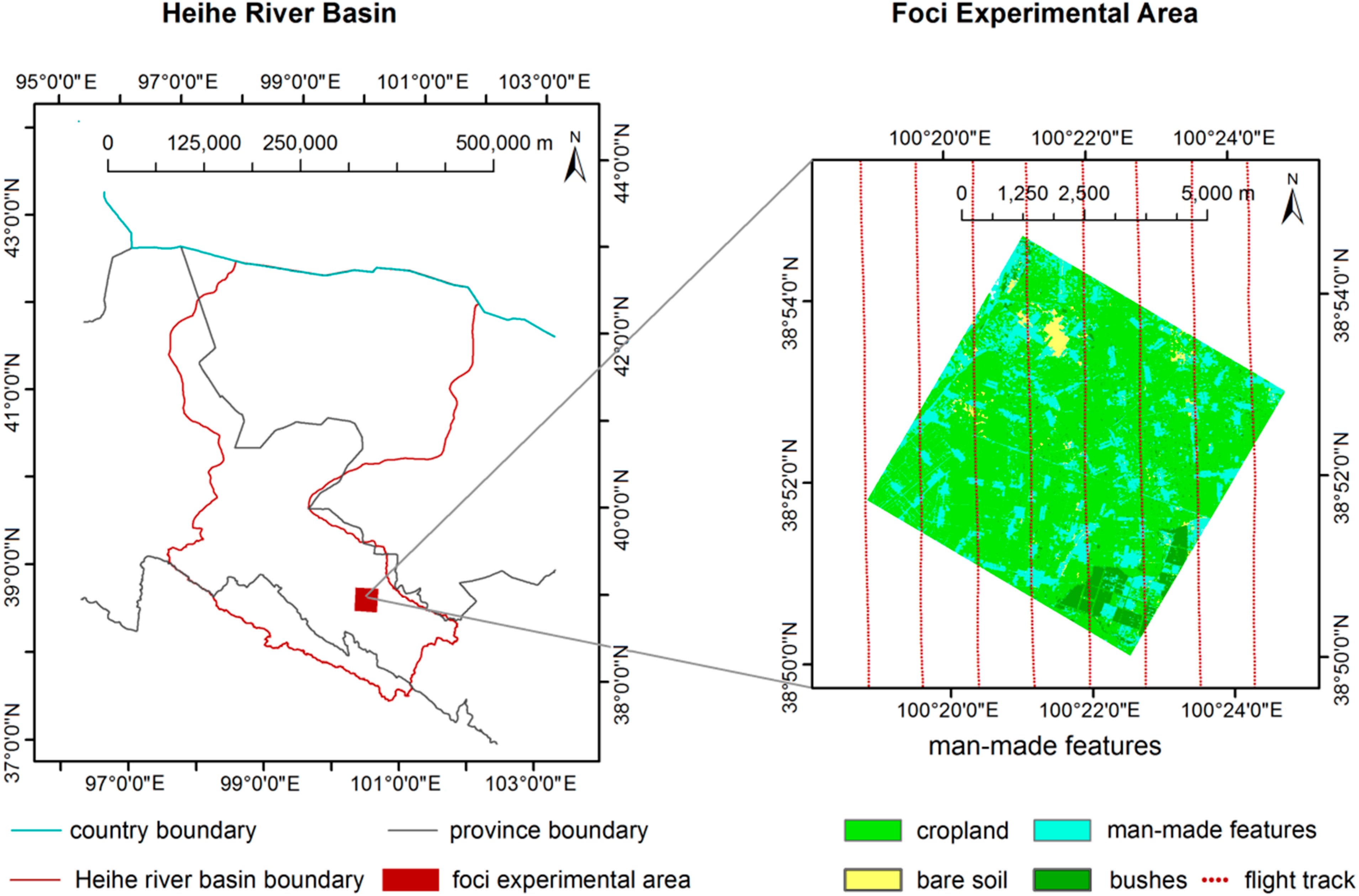
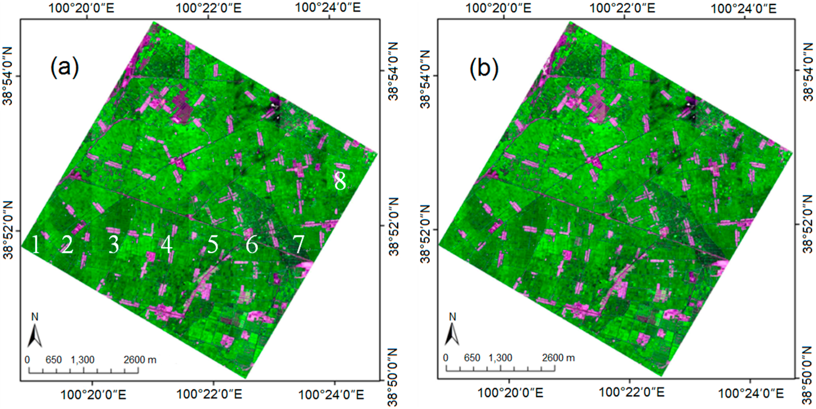
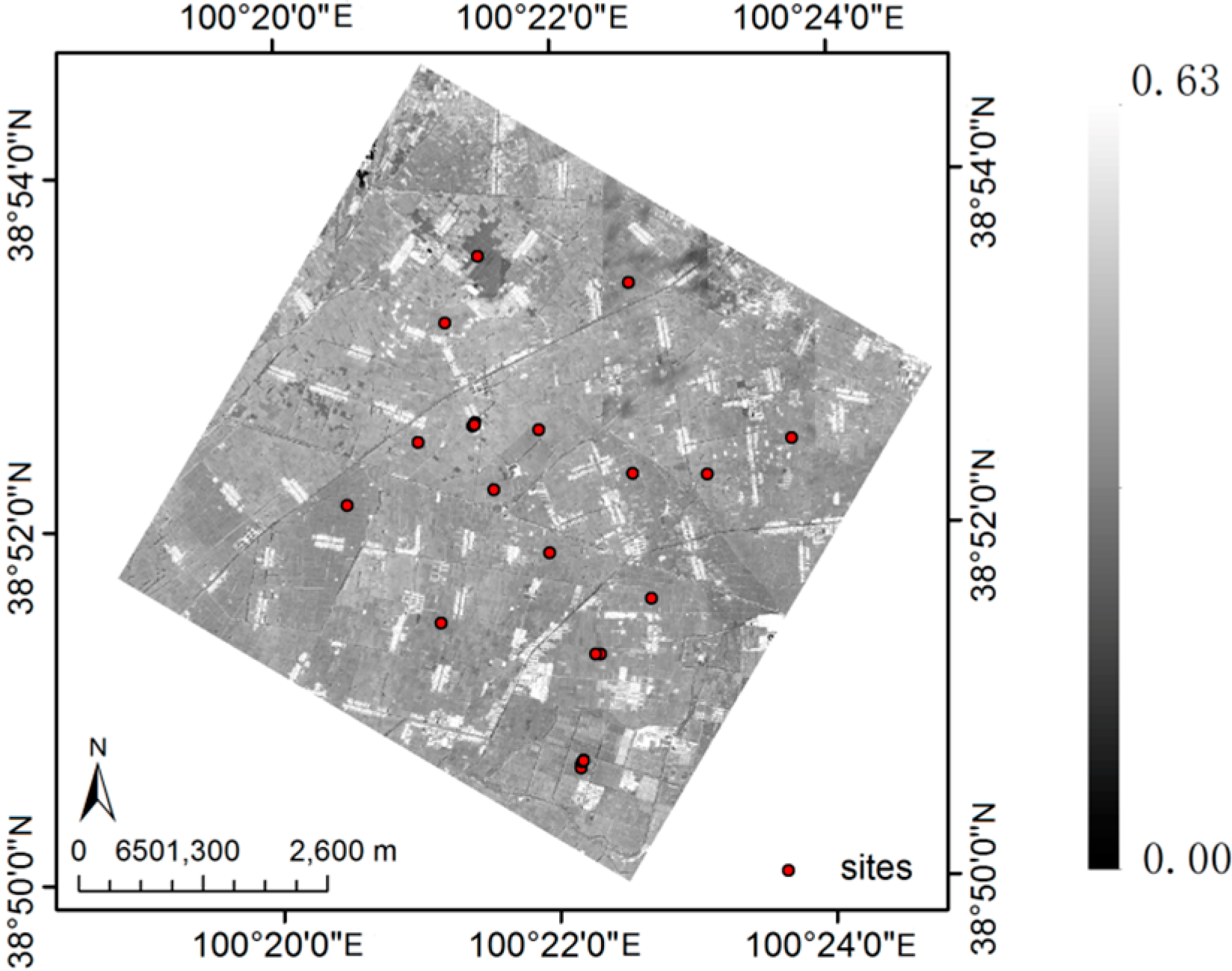
2. A Compact Airborne Spectrographic Imager (CASI)-Based Airborne Experiment in the Heihe Watershed Allied Telemetry Experimental Research (HiWATER)

A CASI-based airborne remote sensing experiment was carried out at FEA (which is located at 38.88°N, 100.36°E) in the middle stream of the Heihe River basin, China, shown in Figure 1, on June 29th 2012, as part of the Heihe Watershed Allied Telemetry Experimental Research (HiWATER). The CASI instrument was a push-broom imaging spectro-radiometer that measured the spectrum of each location on the ground in 48 spectral bands between 380 and 1055 nm. It was flown at a relative altitude of 2 km above the surface and had a field of view (FOV) of 40° with 1500 across-track imaging pixels and a one-meter spatial resolution. The data acquired in this experiment support the inversion of the surface reflectance and related parameters such as the albedo, FPAR, LAI, chlorophyll content, and FVC and can be used to develop scaling methods for multi-spatial resolution remote sensing data [25].
The CASI spectral radiance was converted from digital numbers after spectral and radiance calibration and geometrically corrected to a standard earth-centered coordinate system which was re-sampled at a resolution of 5 m using a UTM projection. With atmospheric parameters measured from the ground, the 6S (second simulation of the satellite signal in the solar spectrum) atmospheric model was adopted to drive the atmospheric parameters that allowed the CASI atmospheric effects to be corrected to obtain the CASI bidirectional function factor (BRF) at the surface [26]. Preliminary validation of the corrected CASI reflectance showed that the absolute differences were 1.5% (relative difference 5.93%) in the visible range of the spectrum (400 nm–700 nm) and 2.5% (relative difference 7.89%) in the near infrared (700 nm–1055 nm), compared with the reflectance of a homogenous concrete surface measured synchronically in the ground campaign.
Figure 1. The Heihe River basin and foci experimental area, showing land classification and the flight track over the FEA.
Remotesensing 07 06784 g001
Land cover types were mapped using the CASI BRF; this classification technique, detailed in the work of Wang et al. [27], is based on the ratio vegetation index (RVI). The FEA contains four land cover types: cropland (mainly corn), manmade features, bare soil, and bushes, as shown in Figure 1. Most of the area is covered by cropland, and its NDVI is generally between 0.75 and 0.88. The narrow range of NDVI indicates a similar structure (growing stage) of the cropland.

3. Deriving the CASI and MODIS (Moderate Resolution Imaging Spectroradiometer) BRDF/Albedo (Bidirectional Reflectance Distribution Function) Algorithm

3.1. Archetypal BRDF

Early field measurements and MODIS observations of the land surface’s anisotropic reflectance show how the characteristics of the BRDF are related to specific land types. Investigations about BRDF features show that the BRDFs within a land cover type have generally similar shapes [13,15,23]. However, for the land type of vegetation, it is more complicated. A rapid change in vegetation properties, which can be indicated by the variation of NDVI, can result in a substantial difference in the BRDF [15,28]. However, the BRDF properties’ dependence on the NDVI is relatively smooth for vegetation classes with high coverage (thus high NDVI) or when the magnitude of the NDVI remains approximately constant within the same land cover type [14,29]. Therefore, it is reasonable to assume that the BRDF’s shape is similar for the same land type of vegetation with a similar NDVI.
The basic shape underlying these BRDFs can be represented by an archetypal BRDF fitted by the kernel-driven model [30] in a normalized form F(Θ,λ) [13,22], as in Equation (1). The archetypal BRDF is a normalized BRDF with a value of one when illuminating and viewing from the nadir. Hence, the archetypal BRDF describes the shape features of the BRDF, but ignores the magnitude.
F ( Θ , λ ) = 1 + f vol ( λ ) f iso ( λ ) × k vol ( Θ ) + f geo ( λ ) f iso ( λ ) × k geo ( Θ )
where Θ is the observation geometry representing the illumination and viewing angles, λ is the wavelength or denotes a waveband with a narrow wavelength width. kvol(Θ) and kgeo(Θ) are the volumetric scattering kernel and the geometric-optical kernel, respectively. fiso(λ), fvol(λ), and fgeo(λ) are the coefficients of the isotropic, volumetric, and geometric-optical scattering, respectively.

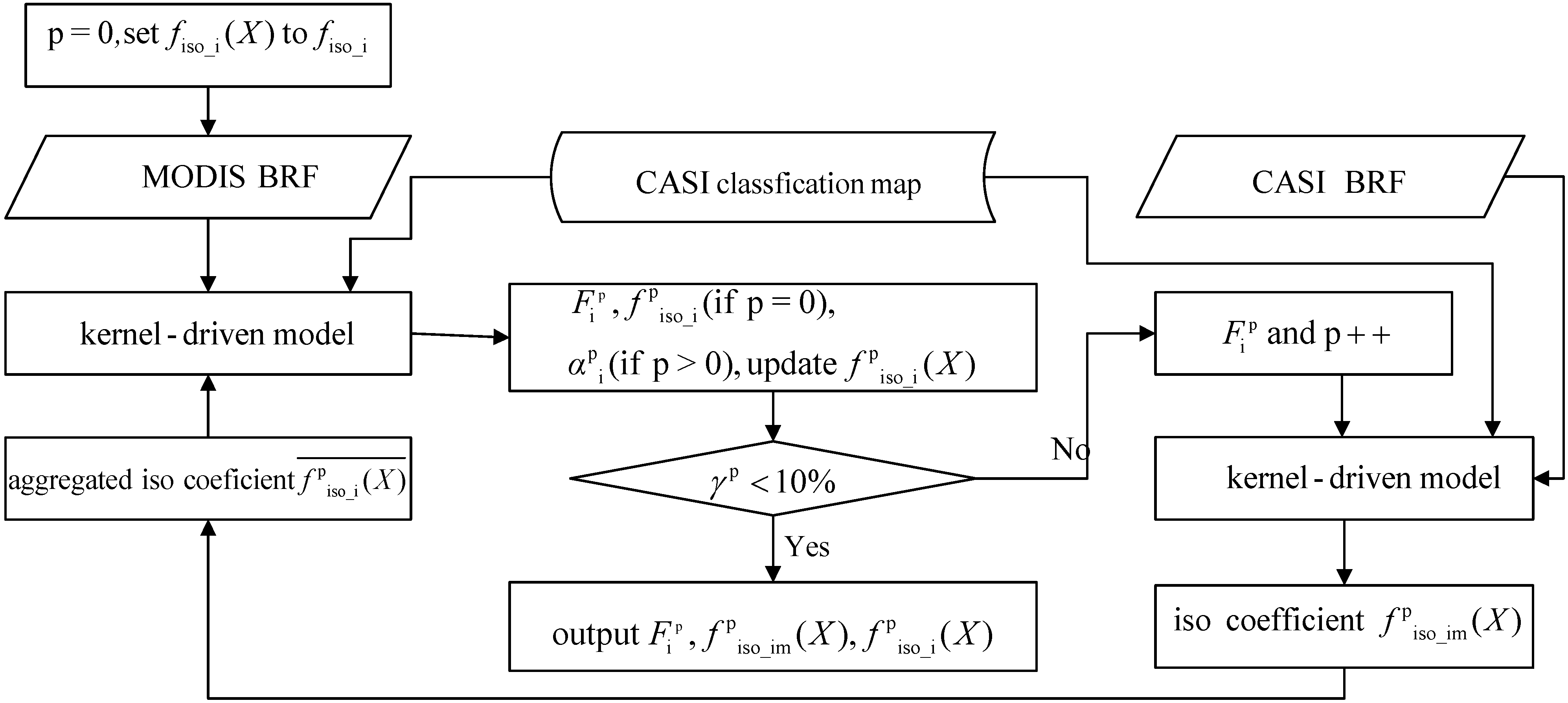
3.2. Land-Type-Based Linear BRDF Unmixing (LLBU) Model Construction

The LLBU algorithm uses airborne fine-scale reflectance and spaceborne coarse-scale reflectance synergistically to determine the fine-scale land-cover-specific archetypal BRDF and the coarse-scale archetypal BRDF on a relatively short timescale. By assuming the land surface BRFs scale linearly in space, the mixed coarse-scale reflectance could be reconstructed by weighting the fine-scale reflectance with the area-based proportion of each land type [16]. LLBU originates in the method of linear spectral unmixing, which uses land type proportions to decompose the coarse-scale mixing BRFs to each land type’s BRF.
In this paper, the daily 500 m reflectance data collected from the MODIS MOD09GA and MYD09GA products on June 29th and 30th were used as the coarse-scale multi-angular reflectance data, which covered the same area and were transformed to the coordinate projection reference frame used by the CASI. This analysis assumes that there are n types of land covering in a MODIS pixel X. Each type is denoted by a subscript i corresponding to the archetypal BRDF Fi(Θ,λ). The MODIS BRF R(Θ,X,λ) can be written as Equation (2).
R ( Θ , X , λ ) = i = 1 n A i ( X ) A × f iso _ i ( X , λ ) × F i ( Θ , λ ) + ξ ( λ )
where X is the MODIS pixel location, A is the MODIS pixel area, Ai(X) is the area of type i in the MODIS pixel X , and ξ(λ) is an error term. It is assumed that there are M CASI pixels for the ith land covering type in MODIS pixel X and that each CASI pixel is indicated by the subscript im . Note that here the parameter λ refers to the sensor’s wavelength, and this is the same for CASI.
The CASI reflectance ρim(Θ’, X, λ) is expressed by Fi(Θ’, λ) with a coefficient fiso_im(X,λ) as follows:
ρ im ( Θ , X , λ ) = f iso _ im ( X , λ ) × F i ( Θ , λ )
where Θ’ represents the CASI observation geometry. It should be noted that the CASI reflectance was convolved to the MODIS VIS and NIR spectral domain using the MODIS band spectral response function. To solve Equation (2), the fine-scale land type and its NDVI were used to derive the land type proportion and the grouped land type BRFs. The least squares error was minimized for all of the clear-sky MODIS observations R(Θ,X,λ) to invert fiso_i(X,λ), the archetypal BRDF Fi(Θ,λ) and fiso_im(X,λ). In the ideal case, in which the two sensors have the same instrumental response and very similar accuracy in the radiation calibrations and atmospheric corrections, the accumulated CASI coefficient f iso_i ( X , λ ) ¯ aggregated from the CASI pixels’ isotropic coefficients and their area aim(X) proportions of land type i equals the isotropic coefficient fiso_i(X,λ) of land type i in a MODIS pixel. However, because there were differences between the two sensors, two more parameters, α i ( λ ) and β i ( λ ) , were used to make the reflectances of the two sensors consistent. The relation of isotropic coefficients between MODIS and CASI was as follows:
f iso _ i ( X , λ ) = α i ( λ ) f iso _ i ( X , λ ) ¯ + β i ( λ ) = α i ( λ ) m = 1 M a im ( X ) A i ( X ) × f iso _ im ( X , λ ) + β i ( λ )

3.3. LLBU Inversion

An iteration strategy was employed for the inversion. In order to keep the consistency of f iso_i ( X , λ ) ¯ and fiso_i(X,λ) for land type i and find an archetypal BRDF Fi(Θ,λ) that fit both the CASI BRF and the land type BRF well, we used the following ratio as an indicator:
γ p ( λ ) = m e a n ( | F i p - 1 ( Θ , λ ) F i p ( Θ , λ ) | F i p - 1 ( Θ , λ ) )
where p is the iteration index. The value of γp(λ) was calculated in a principal plane of several fixed geometries. The threshold of γp(λ) was set to 10%. If γp(λ) met the threshold, the iteration ended. It is noted that the view zenith angle in Θ was limited to values between −60° and 60° due to the poor extrapolation ability of the kernel-driven model for large angles.
The iterative process of inverting the land type’s archetypal BRDF was initialized using Equation (2), and all the BRDFs of type ith are assumed to be the same in MODIS pixels. Thus, the fiso_i(X,λ) are equivalent for all pixels (i.e., fiso_i(λ)). In step 0, all clear-sky observations of MODIS are used to construct Equation (2) to retrieve n types’ BRDF coefficients (fiso_i(λ), fvol_i(λ), fgeo_i(λ)), where the area proportions A i ( X ) A can be pre-calculated by the CASI land cover map. If there are K MODIS pixels and L MODIS images, at most K × L equations (selecting the clear-sky observations) are formulated to solve the 3 × n BRDF coefficients (when p = 0). Once the BRDF coefficients are estimated, they are normalized to obtain the land type’s initial archetypal BRDF coefficients (1, f vol_i ( λ ) f iso_i ( λ ) , f geo_i ( λ ) f iso_i ( λ ) ). In step 1, the land type’s archetypal BRDF coefficients were inserted into Equation (3) to calculate fiso_im(X,λ), where each CASI pixel’s observation is used to construct the Equation (3) to obtain each CASI pixel’s isotropic coefficient fiso_im(X,λ). Then, aggregate fiso_im(X,λ) to update f iso_i ( X , λ ) ¯ with pre-calculated area proportions. In step 2, the newly updated f iso_i ( X , λ ) ¯ , was put into Equation (2) to further invert the land type’s archetypal BRDF coefficients and α i ( λ ) (when p > 0), where there’re also 3 × n unknowns with each type has a corrector α i ( λ ) and two archetypal BRDF coefficients (the volumetric and geometric-optical coefficient, here we denote the them as Fi). In step 3, α i ( λ ) is used to calculate the fiso_i(X,λ) in Equation (4) with the newest f iso_i ( X , λ ) ¯ . Thus, one round of iteration was finished. The new archetypal BRDF are once again put into Equation (3) to update the f iso_im ( X , λ ) as Step 1. Steps 1 to 3 were repeated until γp(λ) met the threshold. The final outputs were the land type’s archetypal BRDF coefficients Fi, the CASI fiso_im(X,λ), which fit the CASI anisotropy reflectance data, and the MODIS f iso_i ( X , λ ) . The LLBU inversion scheme is shown in Figure 2, for simplification, λ is omitted.
Figure 2. The flowchart for the LLBU inversion scheme.
Remotesensing 07 06784 g002

3.4. Albedo Calculation

Land surface albedo, a critical parameter that affects the earth’s climate, is determined by the features of the land surface’s anisotropy reflectance and the atmospheric state. One of the main purposes of the BRDF inversion described in this paper is to improve the airborne CASI and MODIS albedo estimation. The result is expected to keep their values consistent on small timescales. The blue-sky albedo is expressed as a linear combination of the black- and white-sky albedos weighted by the fraction of diffuse sky light in the total illumination, as shown in Equation (6). Integrating the BRDF over the viewing hemisphere results in the black-sky albedo, as in Equation (7); while integrating over the viewing and illumination hemisphere results in the white-sky albedo, as in Equation (8). In the following description, the term albedo refers to the shortwave blue-sky albedo unless otherwise specified.
a ( Θ s , X ) = ( 1 d ) × a dh ( Θ s , X ) + d × a hh ( X )
a hh ( X ) = 1 π 2 π a dh ( Θ s , X ) | Θ s N | d Θ s
a dh ( Θ s , X ) = 1 π λ 1 λ 2 w ( λ ) 2 π f iso ( X , λ ) F ( Θ s , Θ v , X , λ ) | Θ v N | d Θ v d λ
where w(λ) is the spectral weight, N is the unit nadir vector, adh(Θs,X) and ahh(X) are the broadband black-sky albedo and broadband white-sky albedo, respectively, a(Θs,X) is the broadband blue-sky albedo, and d is the fraction of diffuse sky light in the total illumination. The CASI albedo and the MODIS albedo are depicted, respectively, by the isotropy kernel coefficients and archetype BRDF terms in Equation (8).

4. Results

To make the CASI BRF and MODIS BRF datasets consistent, the hyperspectral CASI reflectance was convolved with the MODIS VIS and NIR spectral bands (648 nm, 858 nm, 470 nm, 555 nm) because the CASI covers the spectral range from 380 nm to 1050 nm. The CASI BRF datasets covers the FEA, which corresponding to 153 MODIS pixels. It should be noted that the manmade features in this FEA, including rammed earth buildings, cement buildings and asphalt roads, have relatively smooth surfaces with nearly isotropic reflections. Consequently, a Lambertian BRDF is assigned to this land type.

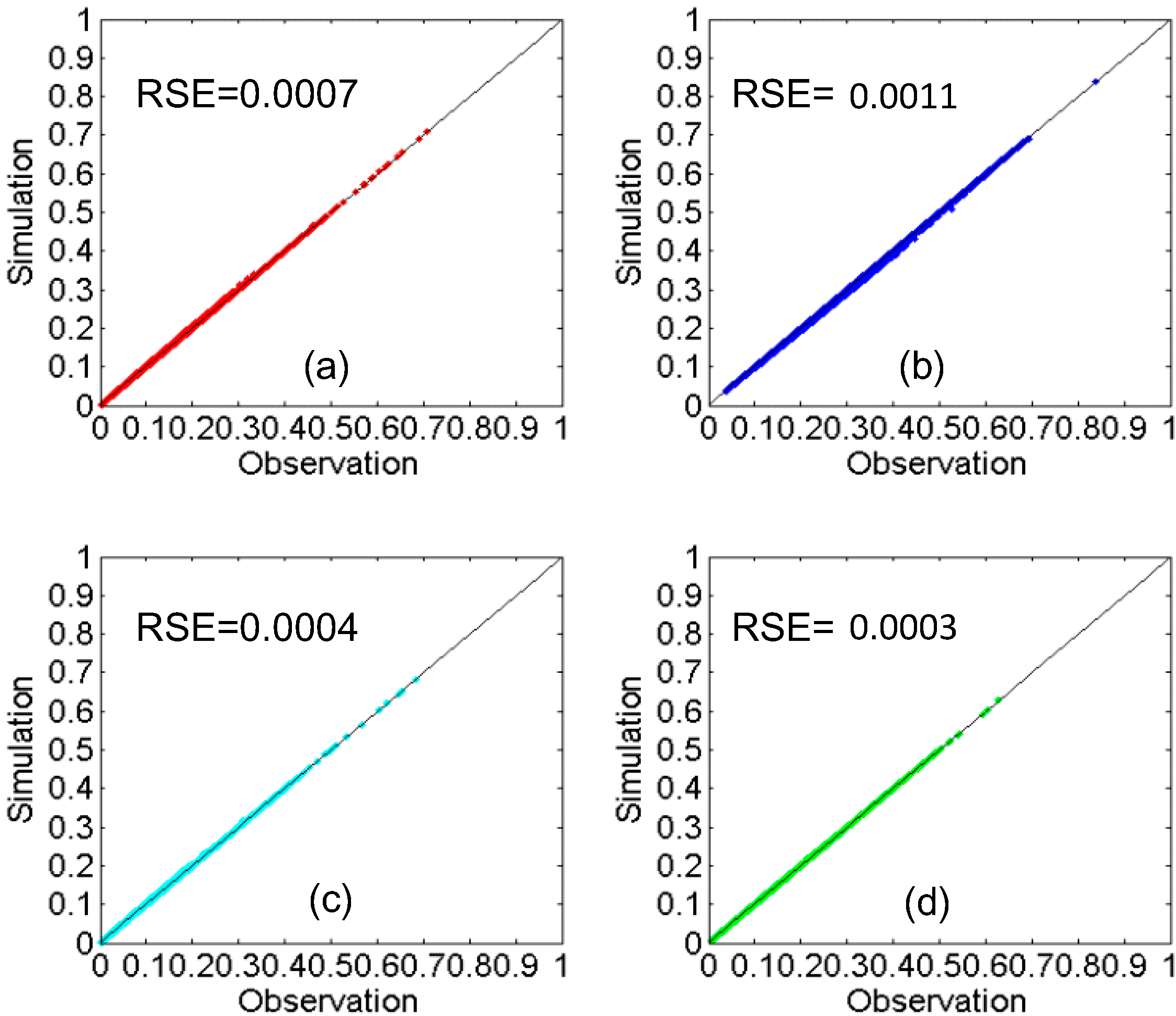
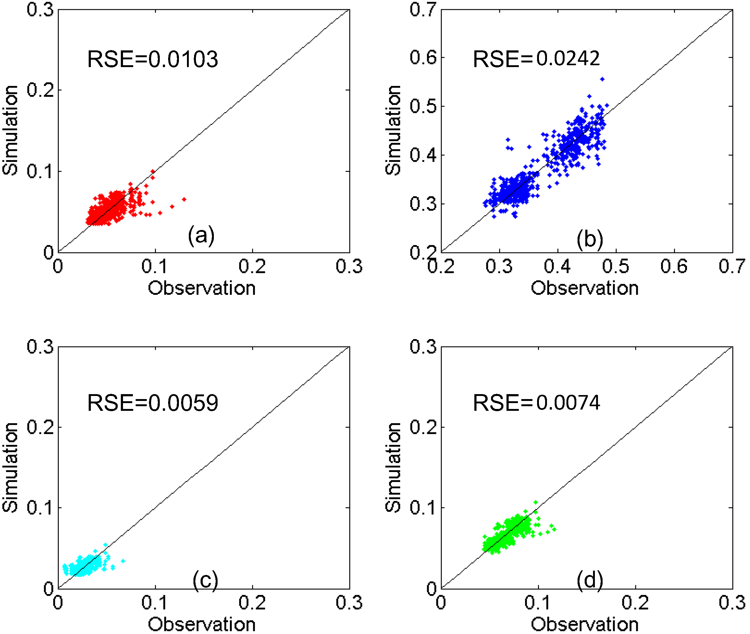
4.1. Investigation of BRF Fitting Ability at Different Scales

LLBU, integrating the MODIS and CASI BRFs to retrieve the BRDF of the two scales, attempts to fit the two sensors observations simultaneously. To investigate the retrieved BRDF, we reconstructed the BRF at both CASI and MODIS scales on their observation geometries and compared the simulations with the observations. The fitting residual standard error (RSE) is used as an indicator.
Figure 3. CASI reflectance comparisons between the simulations and observations: (a) Band 1; (b) Band 2; (c) Band 3; (d) Band 4.
Remotesensing 07 06784 g003
Figure 3 shows the BRF fitting at the CASI scale. The simulations agree very well with the CASI reflectance observations because there is only one angular observation to be fit during the inversion. As in Equation (3), once the land-cover-type specific archetypal BRDF reaches a stable value in the iterative process, the fiso_im(X,λ) from the last p-1 multiplies F i p ( Θ , λ ) , will become significantly closer to the observations. However, for the MODIS scale of LLBU, the fitting shown as in Figure 4 is not as good as the CASI fitting, because it involves multi-pixel and multi-angle observations, as in Equation (2). To evaluate the LLBU fitting at the MODIS scale, we compared it with the counterpart of the AMBRALS algorithm (the algorithm for modeling (MODIS) bidirectional reflectance anisotropies of the land surface) with BRDF parameters from the MODIS BRDF/albedo model parameters product MCD43A1 [31]. MCD43A1 provides the spectral BRDF parameters retrieved from the cloud-cleared Terra and Aqua daily reflectance over 16-day periods. As shown as in Table 1, the RSE of LLBU at the MODIS scale was satisfactory compared with the results of the AMBRALS algorithm.
Figure 4. MODIS reflectance comparisons between the simulations and observations: (a) band 1; (b) band 2; (c) band 3; (d) band 4.
Remotesensing 07 06784 g004
Table 1. The residual standard error (RSE) of fitting the CASI and MODIS reflectances with LLBU or AMBRALS.
RSELLBU CASILLBU MODISAMBRALS MODIS
Band10.00070.01030.0098
Band20.00110.02420.0239
Band30.00040.00590.0084
Band40.00030.00740.0078

4.2. The BRDF Analysis and Assessments

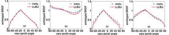
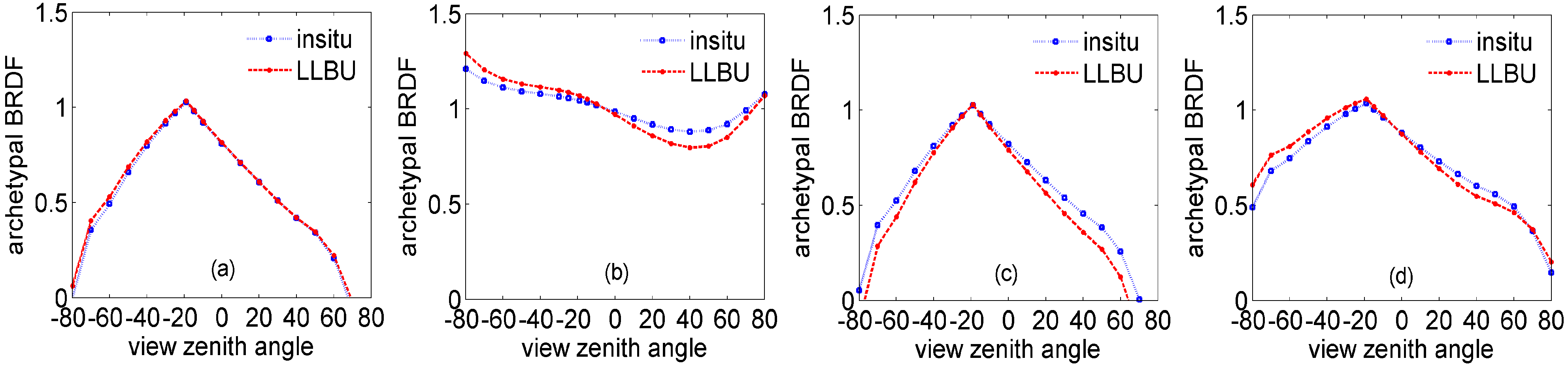
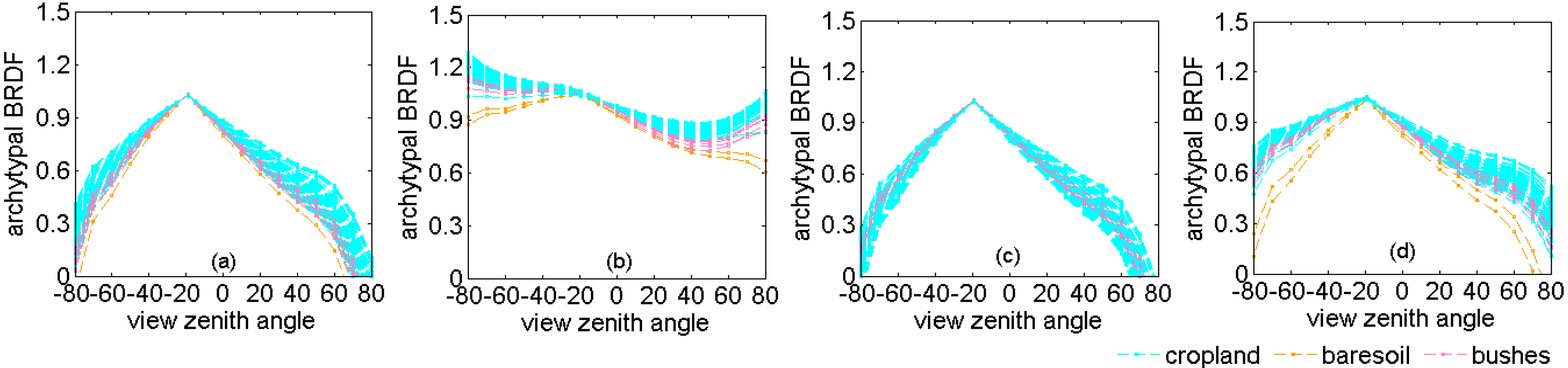
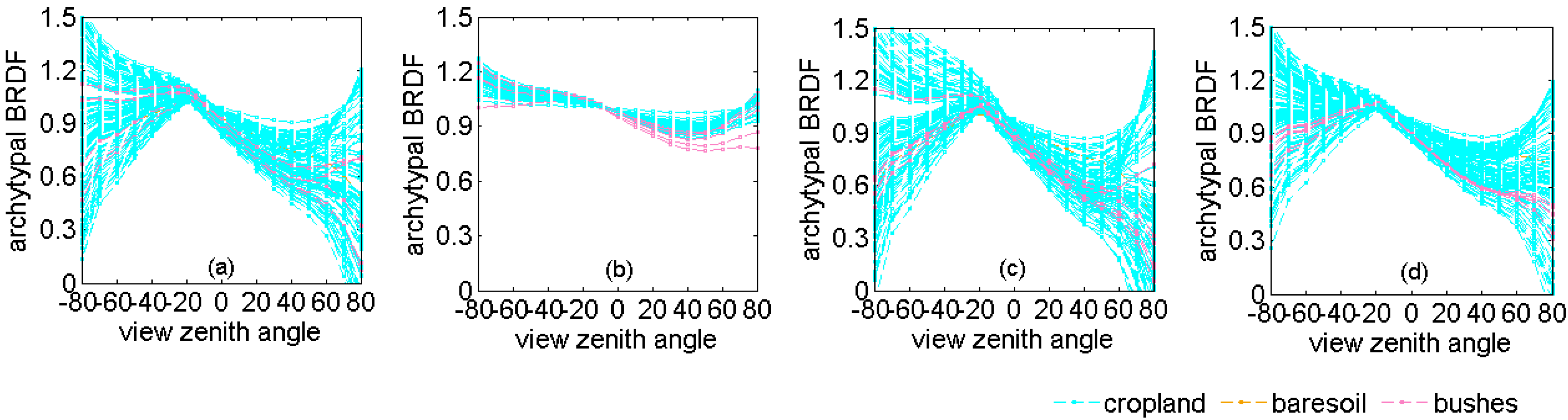
4.2.1. The CASI Land-Type-Specific Archetypal BRDF and Its Comparison with in situ BRDF

Figure 5 shows the retrieved CASI archetypal BRDF of croplands, bare soil and bushes in the principal plane in which the sun zenith angle (SZA) is 19.01°, with Aqua passing on 29 June. The croplands and bushes had very similar BRDF features, i.e., Band 1, Band 3 and Band 4 present significant hotspot effects taking the shape of domes driven by the geometric-optical kernel, while Band 2 (the NIR band) presented a bowl shape due to strong multiple scattering captured by the volumetric scattering component. The bushes showed a more significant hotspot effect than the cropland. For the bare soil, all of the bands had strong hotspot effects with high geometric-optical weights.
Figure 5. The archetypal BRDF shapes in the principal planes. The three columns from left to right are cropland, bare soil, and bushes; the four rows represent Bands 1–4 (al). The sun’s zenith angle for all of these planes is 19.01°; positive (negative) view zenith angles refer to forward (backward) scattering.
Remotesensing 07 06784 g005
To investigate the accuracy of the extracted CASI land-cover-type-specific BRDF, the archetypal BRDF for cropland is compared with the one retrieved from the in situ measured reflectance. The in situ multi-angular BRF measurements were taken in a relatively homogeneous corn field located at 100°22′19.4″E, 38°51′20.3″N on 29 July. The scene of this measurement is shown as in Figure 6. The corn canopy is enclosed with a little gap to the background. A high resolution field portable spectroradiometer (SVC HR-1024) was mounted on a multi-angular controller to make multi-angular observations by changing the view zenith angle. This device observed the target with a view zenith angle step size of 10° from −60° to 60°. The in situ directional reflectance at a cross ridge plane (SZA = 16.3°) and along the solar principal plane (SZA = 25.3°) were measured. These measurements were used to retrieve the kernel-driven model, and then the kernel coefficients were normalized as shown in Equation (1).
Figure 7 compares the LLBU cropland BRDF archetype with the one retrieved in situ along the solar principal plane. The indicator γ cmp ( λ ) as Equation (9) is used to quantify their similarity. The LLBU-retrieved BRDF agreed favorably with the in situ one, as shown in Figure 7. The value of γ cmp in the solar principal planes of Bands 1, 2 and 4 satisfied the threshold requirement of 10%, indicating good agreement, when γ cmp is 2%, 5%, 5%, for those three bands, respectively, except for Band 3, which had a γ cmp of 12%. The discrepancy between the two BRDF shapes in Band 3 may have been partly due to the weak and noisy signal in the blue band in the CASI observations.
γ cmp ( λ ) = m e a n ( | F i LLBU ( Θ , λ ) F i insitu ( Θ , λ ) | F i insitu ( Θ , λ ) )
Figure 6. The scene of corn canopy multi-angular reflectance measurement.
Remotesensing 07 06784 g006
Figure 7. The BRDF shapes in the principal planes retrieved by the in situ measurements and the LLBU. (a) Band 1; (b) Band 2; (c) Band 3 (d) Band 4. The sun zenith angle in these planes is 19.01°; positive (negative) view zenith angles refer to forward (backward) scattering.
Remotesensing 07 06784 g007

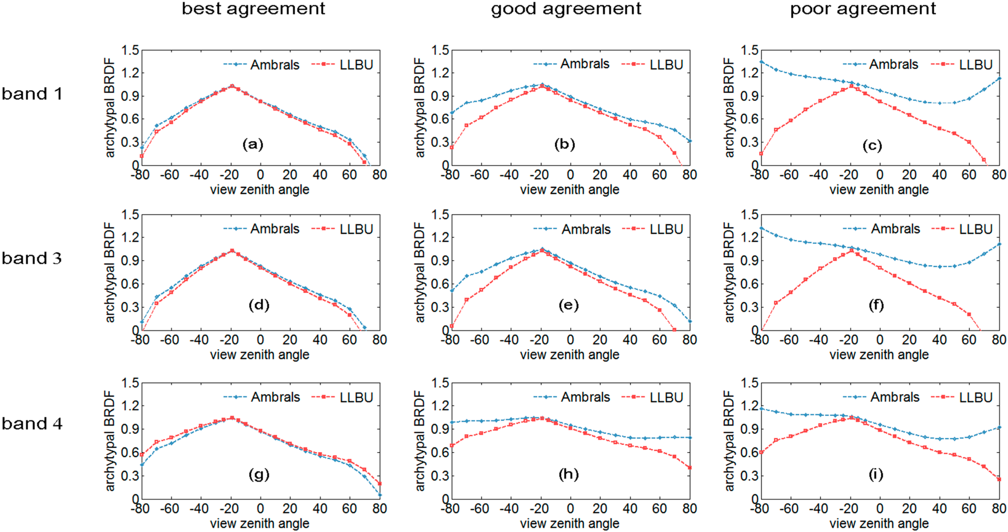
4.2.2. The Archetypal BRDF at MODIS Scale and Its Comparison with MCD43A1 Results

The MODIS pixel’s archetypal BRDF for a spatial resolution of 500 m was calculated from the CASI land-cover-specific archetypal BRDFs weighted by their corresponding area proportions and the isotropy kernel coefficient f iso_i ( X , λ ) which represents the heterogeneity within the class. According to Equation (2), we can describe the MODIS pixel’s archetypal BRDF as follows:
F ( Θ , X , λ ) = i = 1 n A i ( X ) A × f iso_i ( X , λ ) × F i ( Θ , λ ) i = 1 n A i ( X ) A × f iso_i ( X , λ )
Figure 8 presents the archetypal BRDF for all the MODIS’s pixels in the FEA. It specifies the pixels’ dominant land cover type, i.e., the land cover type taking up the largest portion of a MODIS pixel. Figure 8a,b,d shows that these pixels’ BRDF shapes were grouped together very clearly, because they had inherited the land-cover-specific BRDF of their dominant land cover types. There were varieties of the same dominant land-type cover within the archetypal BRDFs due to the effects of other land covers, thus overlapping boundaries appear among groups. In particular, the fuse boundaries between pixels dominated by bushes and those mostly covered by cropland were affected by the second most common land cover type (cropland for the pixels dominated by bushes and bushes for the pixels dominated by cropland). In addition, the archetypal BRDFs for cropland and for bushes were similar in Bands 1, 3 and 4; as shown in Figure 8c, there was no boundary between the two kinds of pixels.
Figure 8. The archetypal BRDFs of the MODIS pixels. (ad) are for Bands 1 through 4, respectively. Different colors mark the largest proportion of a land cover type in the MODIS pixel.
Remotesensing 07 06784 g008
Aside from the different compositions of the land covers, the MODIS pixel BRDF shapes were also affected by the heterogeneity within each class represented by the isotropy kernel coefficient fiso_i(X,λ). Figure 9 shows the isotropic kernel coefficients of the cropland in each MODIS pixel in Band 2. The variety of these coefficients differentiated the cropland growing in the FEA. On the 500 meter scale, the complexity of a MODIS pixel was caused not only by the different abundances of the land covers but also by the heterogeneity within each class. These two factors determine the BRDF shape variance shown in Figure 8.
Figure 9. The isotropic kernel coefficients of the cropland portion of each MODIS pixel in Band 2.
Remotesensing 07 06784 g009
As an indirect evaluation, we compare the LLBU MODIS archetypal BRDF with the MODIS standard product MCD43A1, which is essentially derived by the AMBRALS algorithm. The pixels that were fully invert in AMBRALS and marked as the best quality by MCD43B2 (MODIS BRDF/albedo quality product) were selected. The northwest boundary pixels of the FEA that were adjacent to a desert or river course were eliminated from the comparisons due to geolocation bias.
γ cmp ( X , λ ) = mean ( | F LLBU ( Θ , X , λ ) - F AMBRALS ( Θ , X , λ ) | F AMBRALS ( Θ , X , λ ) )
Figure 10 shows the pixels’ archetypal BRDFs from MCD43A1. The RMSEs of Bands 1 to 4 were 0.19, 0.04, 0.21, and 0.12, respectively. To clarify the comparisons, we used γ cmp ( X , λ ) as Equation (11) to quantify the similarity of the BRDFs of each pixel calculated using LLBU and AMBRALS. For Band 2, all of the pixels were in good agreement, with each pixel’s γ cmp less than 10%. However, the other bands had significant differences for some pixels. Figure 11 shows typical situations for Bands 1, 3 and 4 having the best agreement ( γ cmp 10% ), good agreement ( 10% γ cmp 20% ), or poor agreement ( γ cmp >20% ). However, for Band 4, due to the high values of the archetypal BRDF of MCD43A1, γ cmp ’s threshold for good agreement has been limited to 15%. Table 2 presents the proportion of pixels in each typical comparison case for each band. For Bands 1 and 3, more than 20% of the pixels’ LLBU BRDFs agreed very well with the corresponding AMBRALS results, and 40% of the pixels were in poor agreement. For Band 4, about half of the pixels were in the best agreement, and 24% were in poor agreement. In general, approximately 60% of the pixels were in good agreement for all of the bands.
An important fact is that AMBRALS accumulated multi-angular observations from DOY (day of year) 177 to 192, while LLBU accumulated them from DOY 181 to DOY 182. The AMBRALS value represents the average state over a long period during which the surface may have changed. The spatial distribution of the pixels’ BRDF agreements showed that the ones with a low NDVI variation (e.g., bush-dominated and partly cropland-dominated pixels) were in good agreement. However, bare-soil-dominated pixels were in poor agreement when a significant land cover change occurred during this time period. Figure 12 presents the changes in the land cover of an area that was primarily covered by bare soil on 29 June (DOY 181) and changed noticeably on 8 July (DOY 190). The change in land cover may explain the differences between the AMBRALS and LLBU results. In addition, the vegetation signals in Bands 1 and 3 were very weak, which may have partially brought out the uncertainty in both algorithms.
Figure 10. The archetypal BRDFs of the best-quality marked pixels from MCD43A1, (ad) show bands 1 to 4, respectively.
Remotesensing 07 06784 g010
Table 2. The proportion of pixels in each of the three comparison situations.
Best AgreementGood AgreementPoor Agreement
Band126%37%37%
Band2100%0%0%
Band321%35%44%
Band454%22%24%
Figure 11. LLBU and AMBRALS compared in three typical situations. Columns from left to right are best agreement, good agreement, and poor agreement, respectively, and rows from top to bottom are Band 1 (ac), Band 3 (df), and Band 4 (gi).
Remotesensing 07 06784 g011
Figure 12. Changes in land cover with time. (a) CASI image acquired on 29 June (DOY 181); (b) CASI image acquired on 8 July (DOY 190).
Remotesensing 07 06784 g012

4.3. Visual Assessments of Normalizing the Angular Effects on the CASI Scale

One important application of the land surface BRDF is to normalize multi-angular observations to a standard geometric condition, as it is necessary to take angular effects into account when comparing the long-term reflectance or reflectance-based indices (like NDVI) of pixels acquired with different observation geometries in satellite data [30], and even with airborne data [20]. An anisotropic factor Ω, as in Equation (12), can be used to correct the angular effects [32]. The CASI BRDF was used to normalize the observed CASI reflectance to a standard observation geometry at local noon illumination and nadir view (i.e., θ s =15.71°, θ v =0°, ϕ s =177.15°, ϕ v =0°) with the following Equation (13).
Ω ( θ s , θ v , ϕ s , ϕ v , λ ) = ρ ^ ( θ s , θ v , ϕ s , ϕ v , λ ) ρ ^ ( 0 , 0 , ϕ s , ϕ v , λ )
R ( θ s , θ v , ϕ s , ϕ v , λ ) = Ω ( θ s , θ v , ϕ s , ϕ v , λ ) Ω ( θ s , θ v , ϕ s , ϕ v , λ ) R ( θ s , θ v , ϕ s , ϕ v , λ )
where θ s is the sun zenith angle, θ v is the view zenith angle, ϕ s is the sun azimuth angle,   ϕ v is the view zenith angle, ρ ^ is the simulated reflectance of the BRDF model, and R ( θ s , θ v , ϕ s , ϕ v ) is the normalized reflectance in a standard geometry ( θ s , θ v , ϕ s , ϕ v ) corrected from the observed reflectance R ( θ s , θ v , ϕ s , ϕ v ) in the acquisition geometry ( θ s , θ v , ϕ s , ϕ v ) .
Figure 13. CASI reflectance images. (a) is before normalization, the flight lines are indicated by white-colored numbers; (b) is after normalization.
Remotesensing 07 06784 g013
Figure 13a shows a mosaic of eight different flight cast images (the flight track is shown in Figure 1) before angular normalization. Strong brightness contrasts can be observed where the flight strips were stitched together, revealing the anisotropic effects of the land surface’s reflectance. The eight north-south flight lines were made before local noon when the land was illuminated from the east. Back-scattering occurred when viewing to the west and forward scattering occurred when viewing to the east. The different observation geometry caused the western part of each flight line to be brighter than the eastern part. The anisotropic effects were strong for the six western flight lines (numbered 1–6), but weak for the two eastern lines (numbered 7 and 8). The two eastern lines were flown very near local noon, and thus, there was less difference between the forward and backward directions. In Figure 13b, the angular normalization of the BRDF removed most of the anisotropic effects from the mosaic image. This indirectly shows the good performance of the LLBU-retrieved CASI BRDF parameters.

4.4. Albedo Validation and Comparison

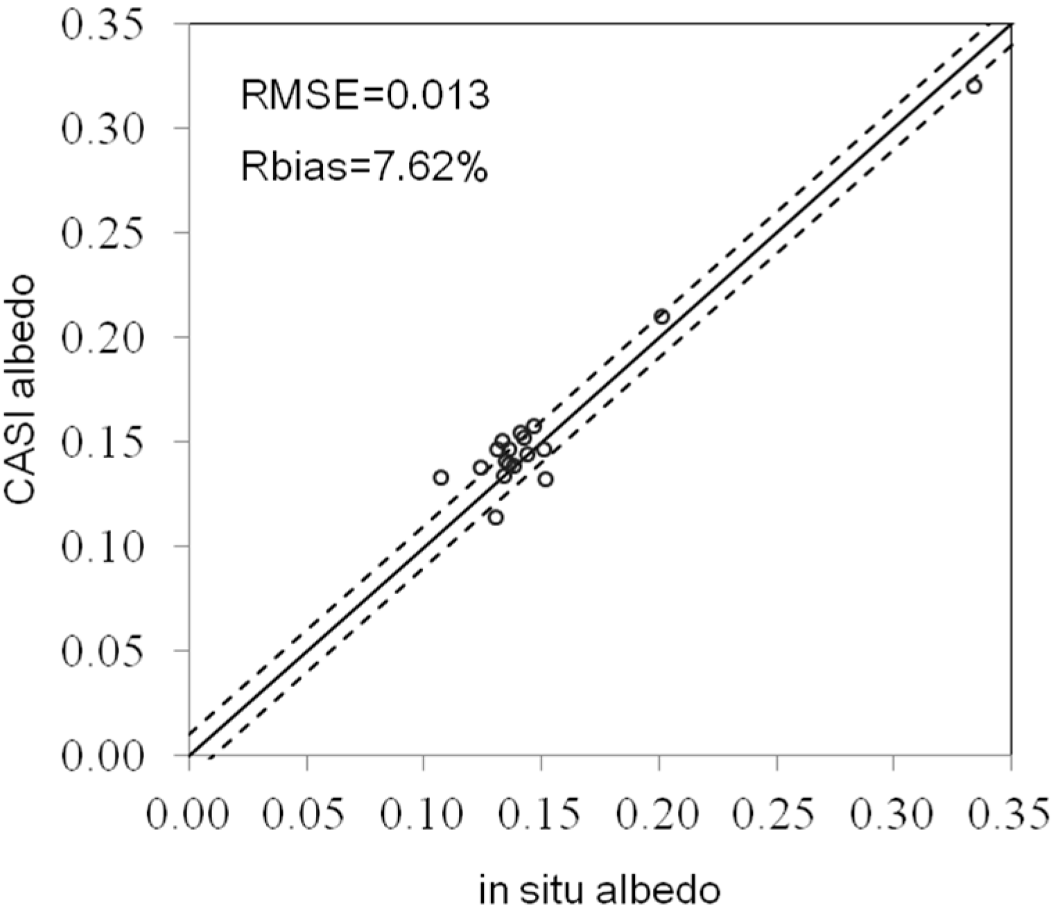
4.4.1. CASI Albedo Validation

The CASI Spectral BSA and WSA were calculated by integrating its BRDF following Equations (6) and (7), where the BSA, which depends on the solar zenith angle, was calculated at local noon. The shortwave albedo was estimated from the spectral albedo by spectral-to-broadband conversion [33] as in Equation (14). Finally, the blue-sky shortwave albedo was interpolated between the shortwave BSA and shortwave WSA weighted by the diffuse skylight fraction d, which was simulated by the atmospheric model 6S with in situ measured aerosol optical depth and water vapor.
α s h o r t w a v e = 0.7738 α 1 + 0.4055 α 2 0.1420 α 3 0.2007 α 4 + 0.0081
where a shortwave is the shortwave albedo and a 1 to a 4 are the spectral albedo of Bands 1 through 4.
Figure 14 shows the CASI shortwave albedo map of the FEA. It has a wide range of values which capture the detailed variations of the land surface albedo on a fine scale.
Figure 14. The CASI albedo of the foci experimental area (red points locate the AWS sites locations).
Remotesensing 07 06784 g014
Kipp and Zonen Net Radiometers (CNR4) mounted on automatic weather station (AWS) towers measured the total downward and upward shortwave radiation (300 nm–2800 nm) and the in situ albedo was calculated as their ratios at local noon. The AWS radiometers were mounted approximately 3 m above the canopy and had a 26 m diameter footprint [34]. The 5 × 5 CASI pixels ( 25m × 25m ) centered on these sites were aggregated to match these sites’ footprints. There are 18 sites distributed in the FEA which are shown in Figure 14. Figure 15 shows the comparisons between the field measurements and the CASI-retrieved albedo. Most of the points are concentrated along the line representing a 1:1 ratio. The RMSE is 0.013 with an average relative absolute bias (Rbias) of 7.62%. These results reveal that the CASI shortwave albedo is quite consistent with the in situ measurements.
Figure 15. Comparisons between the CASI albedo and in situ albedo. The dashed lines show the bias on the interval [−0.01, 0.01].
Remotesensing 07 06784 g015

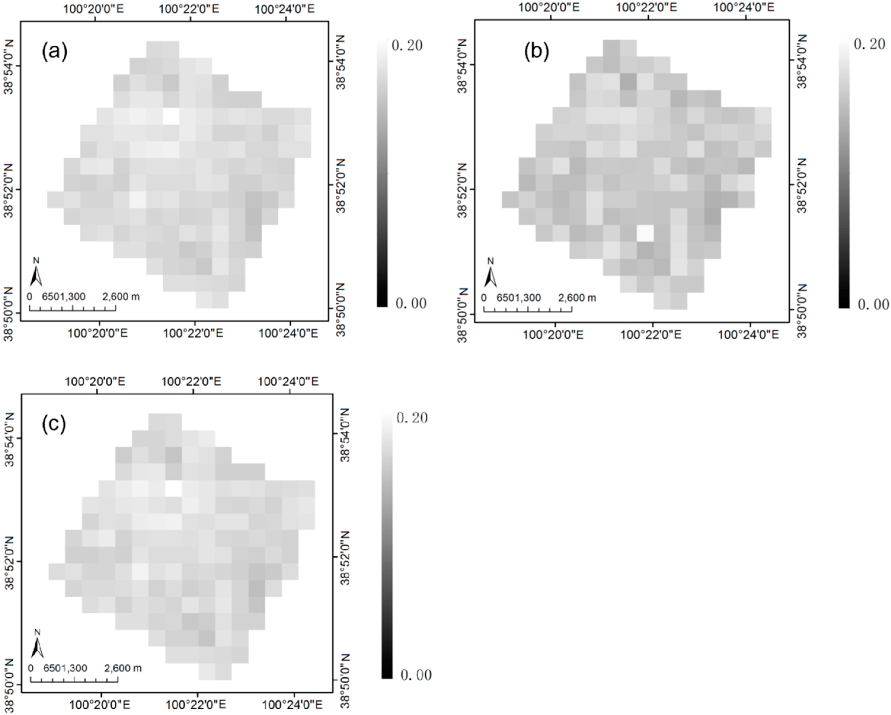
4.4.2. MODIS Albedo Comparison

Figure 16a shows the MODIS albedo derived from the LLBU MODIS BRDF (denoted as MODISLLBU). To quantify the albedo on the MODIS scale, the well-qualified CASI albedo was aggregated to MODIS resolution as a reference albedo (denoted as the CASIagg_ori) shown in Figure 16b. A point spread function (PSF) was applied in the aggregation to account for the spatial characteristics of MODIS, which were approximated by a Gaussian function with a standard derivation of 274 m for MODIS 500 m resolution, as suggested by Barker, et al. [35].
Figure 16. The MODIS albedo. (a) is derived from the MODIS BRDF in LLBU denoted by MODISLLBU; (b) is aggregated from the CASI albedo denoted by CASIagg_ori; (c) is aggregated from the corrected CASI albedo by α i denoted by CASIagg_cor.
Remotesensing 07 06784 g016
Comparing Figure 16a,b shows that these two MODIS-scale albedos had similar spatial distributions. The RMSE is 0.019. Nevertheless, the MODISLLBU image had a higher brightness than the CASIagg_ori image in general (depicted by circles in Figure 17). The MODISLLBU image seems to be a shift of a higher value of approximately 0.02 in comparison to the CASIagg_ori image.
Figure 17. Scatterplots of the MODISLLBU and CASIagg albedos, where circles represent the results from the CASIagg_ori and MODISLLBU images, and crosses represent those from the CASIagg_cor and MODISLLBU images.
Remotesensing 07 06784 g017
The difference between the albedos of the MODISLLBU and CASIagg_ori was due to the difference in reflectance of the two kinds of sensors, which was very obvious during the retrieval of combining the MODIS and CASI BRFs. Table 3 presents the correctors α i ( λ used in Equation (4) for aggregating the CASI isotropic kernel coefficients to MODIS pixels. Furthermore, we applied correctors to the CASI albedo aggregation (denoted as CASIagg_cor) as shown in Figure 16c. MODISLLBU has shown a perfect consistence with CASIagg_cor, as depicted by crosses in the scatterplots shown in Figure 17.
Table 3. The correctors of different land cover types from Band 1 to Band 4.
CroplandManmade FeaturesBare SoilBushes
Band 11.500.450.951.42
Band 21.121.161.251.04
Band 31.460.360.701.45
Band 41.230.570.941.18
According to Equation (4), if the two sensors’ reflectances are comparable, the values of the correctors will be approximately 1. In this paper, the correctors varied with land covers and bands, indicating their different spectral characteristics. This may be explained by the uncertainty of convolving the sparsely sampled hyperspectral CASI reflectance (half of the bandwidth is 7.5 nm) to the MODIS bands, and the uncertainty of the calibration and atmospheric correction in the two sensors. Another important factor was the noise, which could not be avoided, especially in low response bands such as the blue band (Band 3) and the red band (Band 1). This may be a partial explanation of why the correctors for Bands 1 and 3 varied more for the different land covers than those for Band 2.
The correctors for cropland and bushes had values greater than 1, suggesting that a higher reflectance was observed from MODIS than from CASI for the vegetation. Consequently, the MODISLLBU albedo was greater than CASIagg_ori for most of the pixels, as the FEA was mainly covered by vegetation.

5. Discussions

Although the evaluation of LLBU has shown its accuracy in estimating the CASI BRDF and albedo, the bare soil archetypal BRDF may be not so reliable due to the MODIS angular samplings limitation. Considering the land cover change in a period, especially the change of the bare soil shown as in Figure 12, a time window of 5 days before and after the acquired date of CASI data (29 June) was set to collect the MODIS images. Only two days during the eleven-day period around 29 June were clear skies. Therefore, four MODIS images (from TERRA and AQUA on 29 June and 30 June) were used in this retrieval. For the cropland cover, the angular samplings are adequate because cropland is broadly distributed in the MODIS pixels, and thus the BRDF agrees well with the in situ measurements. But as shown in Figure 1, the bare soil coverage was spatially concentrated and mainly occurred in two adjacent MODIS pixels. Narrow angular samples of bare soil, caused by concentrated spatial distribution and a short time of MODIS observations accumulation, reduce the CASI BRDF accuracy to some degree.
Furthermore, the algorithm is applied to retrieve CASI BRDF/Albedo at a spatial resolution of 5 m. Such a fine spatial resolution is assumed to capture the intrinsic length scale of the surface to utilize the kernel-driven model. A 5-meter footprint can well capture the land surface structure of land types like cropland and bare soil in FEA. However, the bushes land type of a single tree at CASI scale may cause some different archetypal BRDF while the bushes are of some grouped trees at MODIS scale. In FEA, the gap of the grouped trees is less than 5 m that leads a mixed canopy in a CASI pixel and thus reduces the archetypal BRDF differences between the CASI and MODIS scales.

6. Conclusions

The LLBU (land-cover-based linear BRDF unmixing) method presented in this paper, combines the spatial information from high-spatial-resolution data to characterize the within-class BRDFs variation, and the multi-angular information from coarse-spatial-resolution data to derivate the land-cover-specific archetypal BRDF. Thus, it determines land surface BRDF at two scales simultaneously. Its unmixing process allows anisotropic reflectance features to be extracted without identifying pure pixels on the coarse scale. In this way, it avoids the limitations of pure pixels or the scale mismatch when using the coarse scale BRDF product as priori-knowledge to estimate the fine scale BRDF in the current methods, especially in heterogonous land surfaces. Compared with the per-pixel retrieval mode of coarse scale data, like MODIS which accumulates multi-angular observations within a 16-day period, LLBU can shorten the length of time for gathering multi-angular information as it involves multi-pixel observations to retrieve.
LLBU was applied to CASI and MODIS in the FEA (foci experimental area) of HiWATER (Heihe Watershed Allied Telemetry Experimental Research). It generates the BRDF and albedo of the two sensors simultaneously. For the CASI scale, its archetypal BRDF is in good agreement with the in situ BRDF for cropland. And the angular effect normalization of the CASI reflectance also indirectly indicates good performance in the BRDF retrieval by LLBU. The CASI albedo has high precision with a RMSE of 0.013 validated by the in situ measurements. On the MODIS scale, the CASI scaled up BRDF with 60% of the pixels have similar BRDF shapes for all bands when compared to the results of the AMBRALS algorithm. Meanwhile, there is a RMSE of 0.019 when compared with the CASI upscaled albedo. These assessments have preliminarily confirmed the good performance of LLBU in general.
LLBU is promising to estimate BRDF\albedo from other high-spatial-resolution data like the spaceborne LANDSAT/TM and HJ-1/CCD, which is important for the regional or local scale study. Nevertheless, several issues within the algorithm itself remain to be addressed. The scaling mechanism of LLBU is based on the geospatial aggregation of subpixels (i.e., CASI) to the coarse-scale pixel (i.e., MODIS). Uncertainties arising from adjacent scattering effects, geo-location precision, classification errors and different spectral responses are all sources of uncertainty in LLBU. Consequently, more evaluations are needed to further assess the performance of LLBU in future.

Acknowledgments

This work was jointly supported by Chinese Natural Science Foundation Project (NO: 41271368, 91125003) and National Basic Research Program of China (2013CB733401).

Author Contributions

Dongqin You and Jianguang Wen mainly wrote the manuscript and were responsible for the research design and result analysis. Qing Xiao, Qinhuo Liu and Jingjing Peng contributed to the CASI airborne experiment design and data collection. Qiang Liu and Yong Tang preprocessed the CASI geometry correction and atmospheric correction. Baocheng Dou contributed to the in situ data collection and participated in the CASI BRDF validation. All of the authors thoroughly reviewed and edited this paper.

Appendix

A. Nomenclature

Θview geometry
sillumination direction
vviewing direction
θ zenith angle
ϕ azimuth angle
λwavelength or waveband
Farchetypal BRDF
kvolvolumetric scattering kernel
kgeogeometric-optical kernel
fiso, fvol, fgeocoefficients of isotropic, volumetric, and geometric-optical scattering
R BRF of MOIDS
X geographical location
iland type index
nnumber of land types
Aiarea of land type i in a MODIS pixel
Aarea of a MODIS pixel
ξerror item
ρBRF of CASI
αi, βithe slope and intercept item of correctors for land type i
γ similarity indicator of BRDF shapes
piteration index
a broad-band blue-sky albedo
a dh broad-band back-sky albedo
a hh broad-band white-sky albedo
ddiffuse sky light fraction of the total illumination
Ω anisotropic factor
ρ ^ simulated reflectance of the BRDF model

B. Abbreviations

AMBRALSthe Algorithm for Modeling (MODIS) Bidirectional Reflectance Anisotropies of the Land Surface
BRDFBidirectional reflectance distribution function
BRFbidirectional function factor
CASICompact Airborne Spectrographic Imager
CARCloud Absorption Radiometer
CCDCharge-Coupled Device
DOYDay of Year
FEAFoci Experimental Area
HiWATERHeihe Watershed Allied Telemetry Experimental Research
HJHuanJing satellite
LAIindex/leaf area index
LBland-type-based
LLBULand-cover-based linear BRDF unmixing
MODISModerate Resolution Imaging Spectroradiometer
MISRMulti-angle Imaging Spectroradiometer
NDVINormalized Difference Vegetation Index
PBPixel-Based
POLDERPolarization and Directionality of Earth Reflectance
RSPResearch Scanning Polarimeter
RVIRatio Vegetation Index
SZASun Zenith Angle
TMThematic Mapper
VZAView Zenith Angle

Conflicts of Interest

The authors declare no conflict of interest.

References

  1. Schaepman-Strub, G.; Schaepman, M.; Painter, T.; Dangel, S.; Martonchik, J. Reflectance quantities in optical remote sensing—Definitions and case studies. Remote Sens. Environ. 2006, 103, 27–42. [Google Scholar] [CrossRef]
  2. Croft, H.; Anderson, K.; Kuhn, N. Reflectance anisotropy for measuring soil surface roughness of multiple soil types. Catena 2012, 93, 87–96. [Google Scholar] [CrossRef]
  3. Chen, J.M.; Leblanc, S.G.; Miller, J.R.; Freemantle, J.; Loechel, S.E.; Walthall, C.L.; Innanen, K.A.; White, H.P. Compact Airborne Spectrographic Imager (CASI) used for mapping biophysical parameters of boreal forests. J. Geophys. Res.: Atmos. 1999, 104, 27945–27958. [Google Scholar] [CrossRef]
  4. He, L.; Chen, J.M.; Pisek, J.; Schaaf, C.B.; Strahler, A.H. Glofbal clumping index map derived from the MODIS brdf product. Remote Sens. Environ. 2012, 119, 118–130. [Google Scholar] [CrossRef]
  5. Li, X.; Strahler, A.H.; Woodcock, C.E. A hybrid geometric optical-radiative transfer approach for modeling albedo and directional reflectance of discontinuous canopies. IEEE Trans. Geosci. Remote Sens. 1995, 33, 466–480. [Google Scholar]
  6. Schaaf, C.B.; Gao, F.; Strahler, A.H.; Lucht, W.; Li, X.; Tsang, T.; Strugnell, N.C.; Zhang, X.; Jin, Y.; Muller, J.-P. First operational BRDF, albedo NADIR reflectance products from MODIS. Remote Sens. Environ. 2002, 83, 135–148. [Google Scholar] [CrossRef]
  7. Bréon, F.-M.; Vermote, E. Correction of modis surface reflectance time series for BRDF effects. Remote Sens. Environ. 2012, 125, 1–9. [Google Scholar] [CrossRef]
  8. Weyermann, J.; Damm, A.; Kneubuhler, M.; Schaepman, M.E. Correction of reflectance anisotropy effects of vegetation on airborne spectroscopy data and derived products. IEEE Trans. Geosci. Remote Sens. 2014, 52, 616–627. [Google Scholar] [CrossRef]
  9. Liang, S.; Stroeve, J.; Box, J.E. Mapping daily snow/ice shortwave broadband albedo from Moderate Resolution Imaging Spectroradiometer (MODIS): The improved direct retrieval algorithm and validation with greenland in situ measurement. J. Geophys. Res.: Atmos. 2005, 110. [Google Scholar] [CrossRef]
  10. Martonchik, J.; Diner, D.; Kahn, R.; Ackerman, T.; Verstraete, M.; Pinty, B.; Gordon, H. Techniques for the retrieval of aerosol properties over land and ocean using multiangle imaging. IEEE Trans. Geosci. Remote Sens. 2002, 36, 1212–1227. [Google Scholar] [CrossRef]
  11. Martonchik, J.; Diner, D.; Pinty, B.; Verstraete, M.; Myneni, R.; Knyazikhin, Y.; Gordon, H. Determination of land and ocean reflective, radiative, and biophysical properties using multiangle imaging. IEEE Trans. Geosci. Remote Sens. 2002, 36, 1266–1281. [Google Scholar] [CrossRef]
  12. Martonchik, J.; Pinty, B.; Verstraete, M. Note on an improved model of surface BRDF-atmospheric coupled radiation. IEEE Trans. Geosci. Remote Sens. 2002, 40, 1637–1639. [Google Scholar] [CrossRef]
  13. Bacour, C.; Bréon, F.-M. Variability of biome reflectance directional signatures as seen by polder. Remote Sens. Environ. 2005, 98, 80–95. [Google Scholar] [CrossRef]
  14. Hautecœur, O.; Leroy, M.M. Surface bidirectional reflectance distribution function observed at global scale by POLDER/ADEOS. Geophys. Res. Lett. 1998, 25, 4197–4200. [Google Scholar] [CrossRef]
  15. Shuai, Y.; Masek, J.G.; Gao, F.; Schaaf, C.B. An algorithm for the retrieval of 30-m snow-free albedo from Landsat surface reflectance and MODIS BRDF. Remote Sens. Environ. 2011, 115, 2204–2216. [Google Scholar] [CrossRef]
  16. Román, M.O.; Gatebe, C.K.; Schaaf, C.B.; Poudyal, R.; Wang, Z.; King, M.D. Variability in surface brdf at different spatial scales (30 m–500 m) over a mixed agricultural landscape as retrieved from airborne and satellite spectral measurements. Remote Sens. Environ. 2011, 115, 2184–2203. [Google Scholar] [CrossRef]
  17. Gatebe, C.K.; King, M.D.; Platnick, S.; Arnold, G.T.; Vermote, E.F.; Schmid, B. Airborne spectral measurements of surface-atmosphere anisotropy for several surfaces and ecosystems over southern Africa. J. Geophys. Res.: Atmos. 2003, 108. [Google Scholar] [CrossRef]
  18. Román, M.O.; Gatebe, C.K.; Shuai, Y.; Wang, Z.; Gao, F.; Masek, J.G.; He, T.; Liang, S.; Schaaf, C.B. Use of in situ and airborne multiangle data to assess MODIS-and Landsat-based estimates of directional reflectance and albedo. IEEE Trans. Geosci. Remote Sens. 2013, 51, 1393–1404. [Google Scholar] [CrossRef]
  19. Knobelspiesse, K.D.; Cairns, B.; Schmid, B.; Roman, M.O.; Schaaf, C.B. Surface brdf estimation from an aircraft compared to MODIS and ground estimates at the southern great plains site. J. Geophys. Res. Atmos. (1984–2012) 2008, 113. [Google Scholar] [CrossRef]
  20. Feingersh, T.; Ben-Dor, E.; Filin, S. Correction of reflectance anisotropy: A multi-sensor approach. Int. J. Remote Sens. 2010, 31, 49–74. [Google Scholar] [CrossRef]
  21. Colgan, M.S.; Baldeck, C.A.; Féret, J.-B.; Asner, G.P. Mapping savanna tree species at ecosystem scales using support vector machine classification and brdf correction on airborne hyperspectral and lidar data. Remote Sens. 2012, 4, 3462–3480. [Google Scholar] [CrossRef]
  22. Sandmeier, S.; Müller, C.; Hosgood, B.; Andreoli, G. Physical mechanisms in hyperspectral brdf data of grass and watercress. Remote Sens. Environ. 1998, 66, 222–233. [Google Scholar] [CrossRef]
  23. Luo, Y.; Trishchenko, A.P.; Latifovic, R.; Li, Z. Surface bidirectional reflectance and albedo properties derived using a land cover-based approach with moderate resolution imaging spectroradiometer observations. J. Geophys. Res.: Atmos. 2005, 110. [Google Scholar] [CrossRef]
  24. Li, F.; Jupp, D.L.; Reddy, S.; Lymburner, L.; Mueller, N.; Tan, P.; Islam, A. An evaluation of the use of atmospheric and brdf correction to standardize landsat data. IEEE J. Sel. Top. Appl. Earth Observ. 2010, 3, 257–270. [Google Scholar] [CrossRef]
  25. Li, X.; Cheng, G.; Liu, S.; Xiao, Q.; Ma, M.; Jin, R.; Che, T.; Liu, Q.; Wang, W.; Qi, Y. Heihe watershed allied telemetry experimental research (hiwater): Scientific objectives and experimental design. Bull. Am. Meteorol. Soc. 2013, 94, 1145–1160. [Google Scholar] [CrossRef]
  26. Vermote, E.F.; Tanré, D.; Deuze, J.-L.; Herman, M.; Morcette, J.-J. Second simulation of the satellite signal in the solar spectrum, 6s: An overview. IEEE Trans. Geosci. Remote Sens. 1997, 35, 675–686. [Google Scholar] [CrossRef]
  27. Wang, Z.; Liu, L. Assessment of coarse-resolution land cover products using CASI hyperspectral data in an arid zone in northwestern China. Remote Sens. 2014, 6, 2864–2883. [Google Scholar] [CrossRef]
  28. Khlopenkov, K.; Trishchenko, A.; Luo, Y. Analysis of brdf and albedo properties of pure and mixed surface types from terra misr using landsat high-resolution land cover and angular unmixing. In Proceedings of the Fourteenth ARM Science Team Meeting, Albuquerque, New Mexico, 22–26 March 2004.
  29. Li, F.; Jupp, D.; Lymburnera, L.; Tana, P.; McIntyrea, A.; Thankappana, M.; Lewisa, A.; Held, A. Characteristics of MODIS BRDF shape and its relationship with land cover classes in Australia. In Proceedings of the 20th International Congress on Modelling and Simulation, Adelaide, Australia, 1–6 December 2013.
  30. Wanner, W.; Li, X.; Strahler, A. On the derivation of kernels for kernel-driven models of bidirectional reflectance. J. Geophys. Res.: Atmos. 1995, 100, 21077–21089. [Google Scholar] [CrossRef]
  31. Strahler, A.H.; Muller, J.; Lucht, W.; Schaaf, C.; Tsang, T.; Gao, F.; Li, X.; Lewis, P.; Barnsley, M.J. MODIS BRDF/Albedo Product: Algorithm Theoretical basis Document Version 5.0. MODIS Doc.. 1999. Available online: http://modis-sr.ltdri.org/publications/MODIS_BRDF.pdf (accessed on 26 May 2015).
  32. Wu, A.; Li, Z.; Cihlar, J. Effects of land cover type and greenness on advanced very high resolution radiometer bidirectional reflectances: Analysis and removal. J. Geophys. Res.: Atmos. 1995, 100, 9179–9192. [Google Scholar] [CrossRef]
  33. Liang, S. Narrowband to broadband conversions of land surface albedo I: Algorithms. Remote Sens. Environ. 2001, 76, 213–238. [Google Scholar] [CrossRef]
  34. Sailor, D.J.; Resh, K.; Segura, D. Field measurement of albedo for limited extent test surfaces. Sol. Energy 2006, 80, 589–599. [Google Scholar] [CrossRef]
  35. Barker, J.; Burelhach, J. MODIS image simulation from landsat TM imagery. Glob. Chang. Educ. ASPRSACSMRT 1992, 92, 156–165. [Google Scholar]

