Article

Adjusted Spectral Matched Filter for Target Detection in Hyperspectral Imagery

1
Key Laboratory of Digital Earth Science, Institute of Remote Sensing and Digital Earth, Chinese Academy of Sciences, Beijing 100094, China
2
School of Geosciences and Info-Physics, Central South University, Changsha 410083, China
3
Department of Electrical and Computer Engineering, Mississippi State University, Starkville, MS 39762, USA
*
Author to whom correspondence should be addressed.
Remote Sens. 2015, 7(6), 6611-6634; https://doi.org/10.3390/rs70606611
Submission received: 25 November 2014 / Revised: 29 April 2015 / Accepted: 8 May 2015 / Published: 26 May 2015

Abstract

:
Supervised target detection and anomaly detection are widely used in various applications, depending upon the availability of target spectral signature. Basically, they are based on a similar linear process, which makes them highly correlated. In this paper, we propose a novel adjusted spectral matched filter (ASMF) for hyperspectral target detection, which aims to effectively improve target detection performance with anomaly detection output. Specifically, a typical case is presented by using the Reed-Xiaoli (RX) anomaly detector to adjust the output of supervised constrained energy minimization (CEM) detector. The adjustment is appropriately controlled by a weighting parameter in different detection scenarios. Experiments were implemented by using both synthetic and real hyperspectral datasets. Compared to the traditional single detection method (e.g., CEM), the experimental results demonstrate that the proposed ASMF can effectively improve its performance by utilizing the result from an anomaly detector (e.g., RX), particularly in situations with a complex background or strong anomalies.

Graphical Abstract

1. Introduction

Hyperspectral imaging (HSI) provides significant information about spectral characteristics of materials in the surface of the Earth [1]. Due to high spectral resolution, each pixel (considered as a vector) in a hyperspectral dataset can be seen as a “fingerprint” of the underlying materials within the spatial point. Based on these spectral signatures, HSI has extraordinary potential to identify small targets of interest [2]. The targets, as mentioned here, are primarily man-made objects or objects with signatures being spectrally distinct from image background, which are generally embedded in a single pixel area and cannot be easily identified by visual inspection [3]. The major objective of hyperspectral target detection is to detect these targets by exploiting the spectral signatures of the materials. As a result, over the last decade, target detection has received considerable interest in the HSI community, and has been widely used in reconnaissance and surveillance related applications [4,5].
In general, detection algorithms can be divided into two categories [6,7,8]. One is with known target signature, which to directly decide whether or not the pixel is a target. Another is anomaly detection, which is to search pixels whose spectral signatures are different from their surrounding background.
In supervised target detection, the target spectral characteristics are often defined by a single target spectrum [9] or a target subspace [10]. Spectral matched filter (SMF), as a standard technique, is widely used in detecting objects of interest in HSI [11]. SMF is based on the assumption of a linear model where the spectral signature of the target and the background clutter covariance matrix are assumed to be known. Another well-known signature-based approach is constrained energy minimization (CEM) [2], where a finite impulse response (FIR) filter is designed to maintain the desired target while minimizing the entire image output energy. In contrast to SMF, the use of correlation matrix in CEM may be easier to be implemented in real-time processing [12,13]. The orthogonal subspace projection (OSP) algorithm [14,15] is based on maximizing the signal-to-noise ratio (SNR) of the target in the subspace orthogonal to the background. Other matched subspace detectors (MSD) can also be derived from the generalized likelihood ratio test (GLRT) by constructing different subspace models [16,17,18]. In [10], an adaptive matched subspace detector was introduced, which is now called adaptive coherence estimator (ACE). Additionally, all the above target detectors can be extended to their corresponding nonlinear versions through the use of a kernel-based approach [19,20].
In anomaly detection, no prior knowledge of the target spectral signature is used. In [21], a spectral anomaly detection algorithm was developed for detecting targets of unknown spectral distribution. This algorithm is now commonly referred to as the Reed-Xiaoli (RX) anomaly detector which has been successfully applied to many hyperspectral anomaly detection applications [22]. It is considered as the benchmark anomaly detection algorithm. Several variations of the RX detector have been proposed in the literature [12,23,24,25,26]. As an example, in [12], a modification to the RX algorithm was derived by substituting the correlation matrix for the covariance matrix, so that RX can be implemented in real-time more easily. A subspace model has also been investigated in anomaly detection [27]. In subspace anomaly detectors, the input spectra are projected onto a subspace, whose bases are defined by some projection vectors. Both subspace and RX anomaly detectors intend to suppress the background clutter. Similar to the signature-based supervised target detectors, all the aforementioned anomaly detectors can be extended to corresponding kernel-based nonlinear versions as well [28,29].
Signature-based target detection and anomaly detection generally are considered as two independent tools. However, it is easy to find that there are inextricable links between these two kinds of algorithms. This is due to the fact that they are based on a linear process that exploits the first or second order statistics to identify targets, estimating the background covariance matrices or their corresponding subspaces [6,30]. Based on this observation, target and anomaly detectors can be considered as detection pairs, in which, target detection performance can be improved by considering anomaly detection output. In this paper, we analyze the connections in a typical detector pair (i.e., the CEM and RX algorithms), and, specifically, we propose an adjusted spectral matched filter (ASMF) to improve the performance of CEM target detection by adjustment according to the corresponding RX anomaly detector. Note that both CEM and RX utilize the second order statistics, although high-order statistics may offer some advantage [31].
The remainder of this paper is organized as follows. Section II briefly describes CEM and RX algorithms. In Section III, the ASMF is proposed by combining the CEM and RX. Section IV conducts a detailed evaluation of the proposed method using synthetic data. Section V performs experiments using real hyperspectral datasets. Finally, section VI draws the conclusion.

2. CEM and RX Algorithms

In this section, we provide a short overview of the CEM and RX algorithms. One is a classical method in supervised target detection, and the other is the benchmark of anomaly detection.

2.1. CEM Algorithm

Given a finite set of observations S={r1,r2,…,rN}, where ri=(ri1,ri2,…,riL)T for 1 ≤ iN is a sample pixel vector. Suppose that the desired signature d is also known a priori. The objective of CEM is to design a FIR linear filter with L filter coefficients {w1,w2,…,wL}, denoted by an L-dimensional vector w=(w1,w2,…,wL)T that minimizes the filter output energy subject to the following constraint:
d T w = l = 1 L d l w l = 1
Let yi denote the output of the designed FIR filter resulting from the input ri. Then yi can be written as:
y i = l = 1 L w l r i l = w T r i = r i T w
Therefore, the average output energy produced by the observation set S and the FIR filter with coefficient vector w=(w1,w2,…,wL)T specified by Equation (2) is given by:
1 N [ i = 1 N y i 2 ] = 1 N [ i = 1 N ( r i T w ) T r i T w ] = w T ( 1 N [ i = 1 N r i r i T ] ) w = w T R w
where R = 1 N [ i = 1 N r i r i T ] turns out to be the L × L sample autocorrelation matrix of S.
Minimizing Equation (3) with the filter response constraint d T w = l = 1 L d l w l = 1 yields:
min w 1 N [ i=1 N y i 2 ]= min w { w T R w } subject to  d T w=1
The solution to Equation (4) was shown in [2] and called CEM detector with the weight vector w* given by:
w * = R 1 d d T R 1 d
Thus, the CEM algorithm can be written as:
CEM ( x ) = w * T x = ( R 1 d d T R 1 d ) T x = x T R 1 d d T R 1 d

2.2. RX Algorithm

The RX algorithm is given by:
RX ( x ) = ( x u b ) T 1 ( x u b )
where ub is the estimated background mean vector and ∑ is the estimated background covariance matrix, which can be estimated globally from the whole hyperspectral image or locally with a dual-window. In this research, the global detection is applied. To estimate ∑ globally, the background pixels are usually modeled as a mixture of multivariate Gaussian distributions. The RX(x) in Equation (7) actually is a measure that calculates the well-known Mahalanobis distances. Mathematically, RX also can be considered as an inverse operation of the principal components analysis.
Furthermore, in order to improve the performance of CEM, our interest is focused on a simplified RX version which was introduced in [12] by replacing the sample covariance matrix by the sample correlation matrix. As a result, the RX algorithm can be also written as:
RX ( x ) = x T R 1 x
which uses x and R−1 in place of (x-ub) and ∑−1, respectively, so that RX can be easily implemented in real-time without updating the sample mean, and there is no visible and appreciable difference for RX to use ∑−1 or R−1 [32].

3. Adjusted Spectral Matched Filter

In the section, we further analyze the relationship between CEM and RX. By taking advantage of their respective features, we build a novel ASMF algorithm for target detection.

3.1. The Relationship between CEM and RX

It is important to note that the target detection result generated by the CEM algorithm can be visualized as a grayscale image, in which, the higher the probability of detecting a target, the greater the output value of the pixel. Targets are claimed in terms of the value returned by CEM, so that the pixel with the highest value of CEM(x) will be considered the first target, and so on. Notice the denominator in Equation (6) is a constant, so the CEM can be written as:
CEM ( x ) = x T R 1 d M
where M=dTR−1d as a constant can be discarded. Thus, we can easily find that there is a close relationship between the formula xTR−1x of RX and the numerator xTR−1d of CEM.
These two processes can be written as (xTR−1/2)(R−1/2x) and (xTR−1/2)(R−1/2d) separately [33], and both of them can be considered as a two-step processing. The first step is projecting the signal x into the operator R−1/2. This step represented as xTR−1/2 constrains the background into a very low level (to eliminate principal component) while retaining or amplifying anomalous signatures. In the second step, RX returns the energy of xTR−1/2 directly, while CEM calculates the energy of xTR−1/2 by projecting it onto R−1/2d. This means, by CEM, those pixels similar to the target signature will be amplified and that do not match the target signature will be suppressed again. In other words, through this step, CEM can extract the targets from a set of anomalies (which are potential targets).
However, CEM cannot always generate a satisfactory result. In some situations, the operator R−1/2 is only with difficulty able to suppress all the background energies effectively, and there may be some low probability objects maintaining great power [34,35]. Sometimes, the energy of an anomaly (which unfortunately is not a target) is too strong to be constrained under the desired target level, which leads to false alarm.
A practical detection experiment is used to illustrate this circumstance. When detecting a real target in a dataset [36] as shown in Figure 1, the CEM output includes many unacceptable false alarms, as shown in Figure 2a. On the other hand, by performing the RX anomaly detection, we can see that the greatest false alarm in the CEM output is also the strongest anomaly in the result of RX, as shown in Figure 2b. Here is the dilemma: we detect targets through a supervised target detection algorithm but are interfered by many unwanted anomalies, while we detect all the anomalies through anomaly detection but do not know which one is the desired target. It is expected that the proposed ASMF can resolve such a dilemma.
Figure 1. 3D cube of the Target Detection Self-Test dataset including HyMap reflectance images of Cook City in Montana, USA, cover an area of 280 × 800 pixels with 126 spectral bands.
Remotesensing 07 06611 g001
Figure 2. Hyperspectral image target detection results, where (a) is CEM result and (b) is RX result.
Remotesensing 07 06611 g002

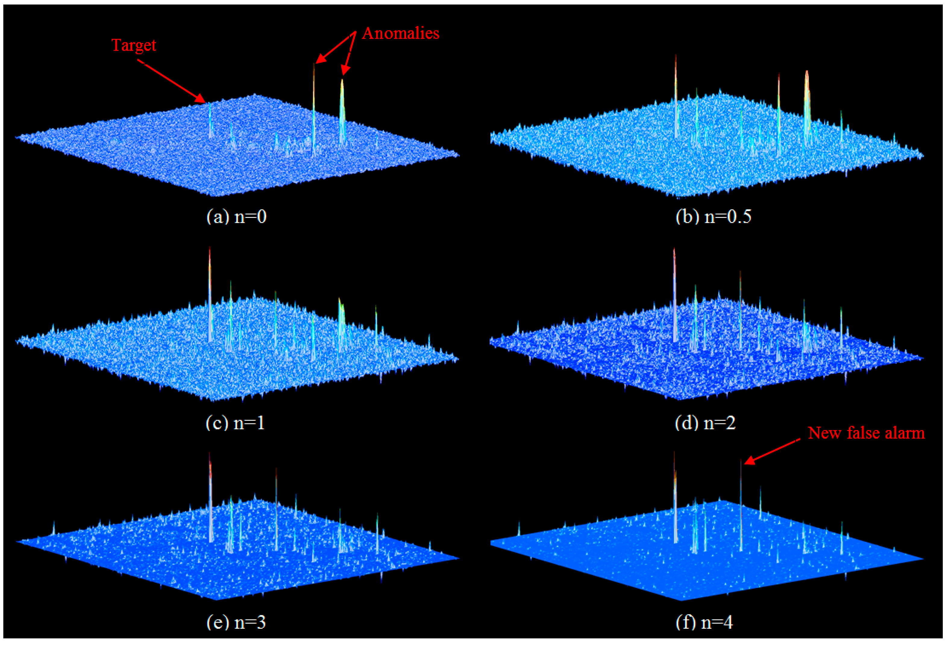
3.2. Adjusted Spectral Matched Filter

As shown in Figure 2, both the CEM and RX detectors constrain most pixels in the scene to a very low level with regard to background pixels. For abnormal pixels, due to the constraint of the target vector, the output of CEM is decreased relatively compared to the RX output. Only for the target pixels, the output of CEM may be increased. Therefore, even if there are many abnormal pixels with large output energy, by comparing the results of CEM and RX, we can determine whether the anomaly is a true target or a false alarm. In this way, we can construct a comparing factor for the outputs of target and anomaly detectors pixel-by-pixel. Finally, this factor is used as a feedback to adjust the results of CEM to increase the reliability of target detection.
For the CEM and RX algorithms, we construct a factor for the ASMF as A = | x T R - 1 d x T R - 1 x | . Furthermore, a weighting factor n is added to A so that we can control the strength of the adjustment. Thus, the ASMF is expressed as:
ASMF( x )=CEM( x ) A n
where CEM ( x ) = x T R 1 d d T R 1 d is the output of CEM, An as an adjusting factor shows the likelihood of an anomaly being a target, and n is a predefined power (which can be simply 1 or 2). Obviously, by this adjustment, those pixels similar to target and have been extracted by CEM, will be amplified again; but those non-target pixels with large anomalous energy will be reduced.
Since background energy has been reduced to a low level due to the constraint in CEM, the adjusting factor A aims to enhance real targets from the potential ones. Thus, factor A with a larger weight n can increase the separability between the real targets and other anomalous pixels, which would generate better detection performance. However, due to the diversity of background and the existence of noise, significantly increasing the weight n may also amplify non-target pixels, resulting in new false alarms. To illustrate this phenomenon, the ASMF with different values of n are tested in the real hyperspectral dataset (Figure 1). As shown in Figure 3, the weight n is set to 0, 0.5, 1, 2, 3, and 4, respectively. When n is set to 0, the ASMF becomes the CEM algorithm, and there are two main anomalous outputs greater than the target (Figure 3a). When n = 0.5, the target output is obviously enhanced but still less than the anomalies (Figure 3b). With the increased n, the proposed ASMF method compresses the outputs of anomalies to smaller values, which is helpful to highlight the targets. Unfortunately, when the weight n continues to increase (such as n = 4), some background pixels are amplified to a high level, as shown in Figure 3f. To quantitatively evaluate the detection performance of using different n, the receiver operating characteristic (ROC) curves [37] are adopted. As shown in Figure 4, the detection performance rises continuously from n = 1 to n = 2, and the performance of n = 3 is close to that of n = 2. However, when the weight n exceeds a threshold value (n = 4 in this experiment), the performance of ASMF begins to degrade. Therefore, we choose 1 and 2 as the parameter of ASMF, which provide stable detection performance.
In addition, we compare the computational complexity of five different methods which are CEM, RX (using covariance matrix and correlation matrix respectively), ASMF with n = 1, and ASMF with n = 2. The computing times of each algorithm obtained by a MATLAB program in the real data detection (Figure 1) are listed in Table 1. The computer utilized in the experiments is equipped with an Intel Core 2 Quad CPU with 2.5 GHz and 4 GB of main memory. As we can observe from this table, the CEM detection is faster than RX using covariance matrix, but the RX (using correlation matrix) without moving the mean value will be slightly faster than CEM. The computing time of ASMF is longer than both CEM and RX, but it is still acceptable for actual applications.
Figure 3. 3-D plots of the detection results for the HyMap dataset by implementing different weight n in ASMF.
Remotesensing 07 06611 g003
Figure 4. ROC curves corresponding to the detection results reported in Figure 3.
Remotesensing 07 06611 g004
Table 1. Computing time of five algorithms in the detection of the HyMap real data.
AlgorithmCEMRX Using Covariance MatrixRX Using Correlation MatrixASMF n = 1AMSF n = 2
Computing time3.90 s4.06 s3.80 s6.75 s6.86 s
It is worth mentioning that, when n = 1, x T R 1 d d T R 1 d | x T R 1 d x T R 1 x | has a similar but different form with ACE, which is ACE ( x ) = ( x T R 1 d ) 2 ( d T R 1 d ) ( x T R 1 x ) . Their difference will be demonstrated in the following experiments. Furthermore, both the CEM and RX algorithms can be restructured by changing the correlation matrix to covariance matrix and the proposed ASMF method can also be applied.

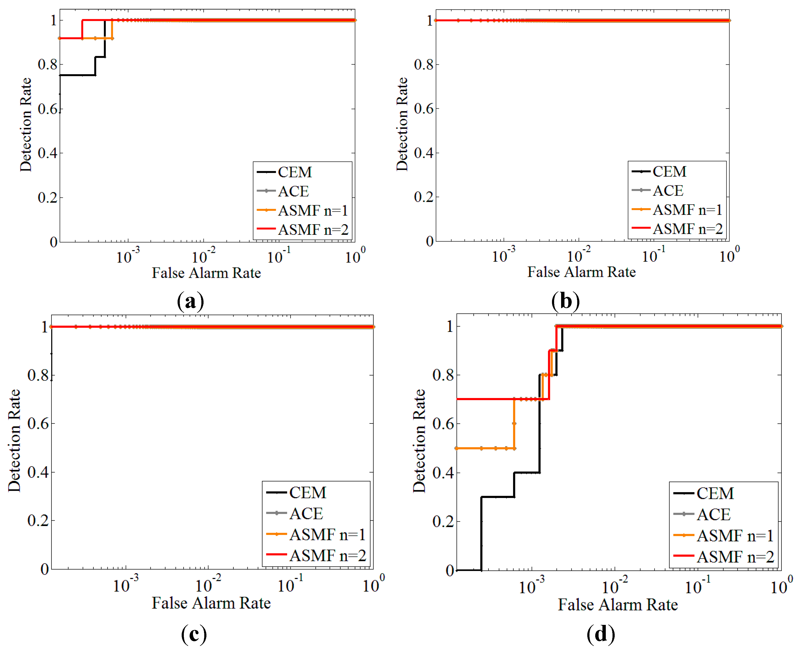
4. Experiments with Synthetic Data

To demonstrate the performance of ASMF, synthetic data are used first. As shown in Figure 5, an airborne visible/infrared imaging spectrometer (AVIRIS) [38] dataset covers an area of 320 × 320 pixels, and its spatial resolution is approximately 5 m. The image has 224 spectral channels in wavelengths ranging from 370 to 2510 nm, in which the wavelengths of 1350–1420 and 1810–1940 nm are water-absorption bands and removed in the experiments. To generate synthetic data, specific targets were implanted into this scene.
Figure 5. 3D cube of the AVIRIS dataset cover a farmland area of 320 × 320 pixels with 193 spectral bands.
Remotesensing 07 06611 g005

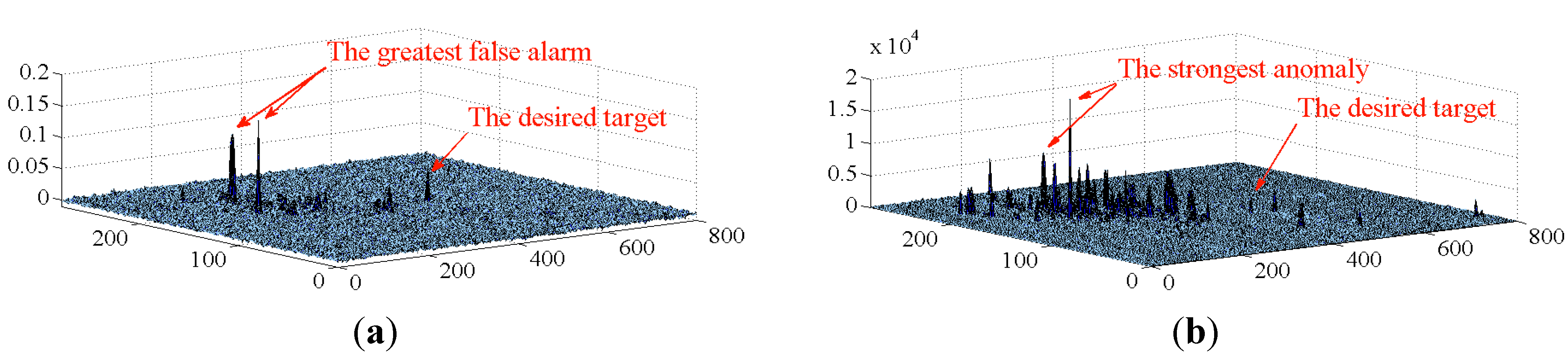
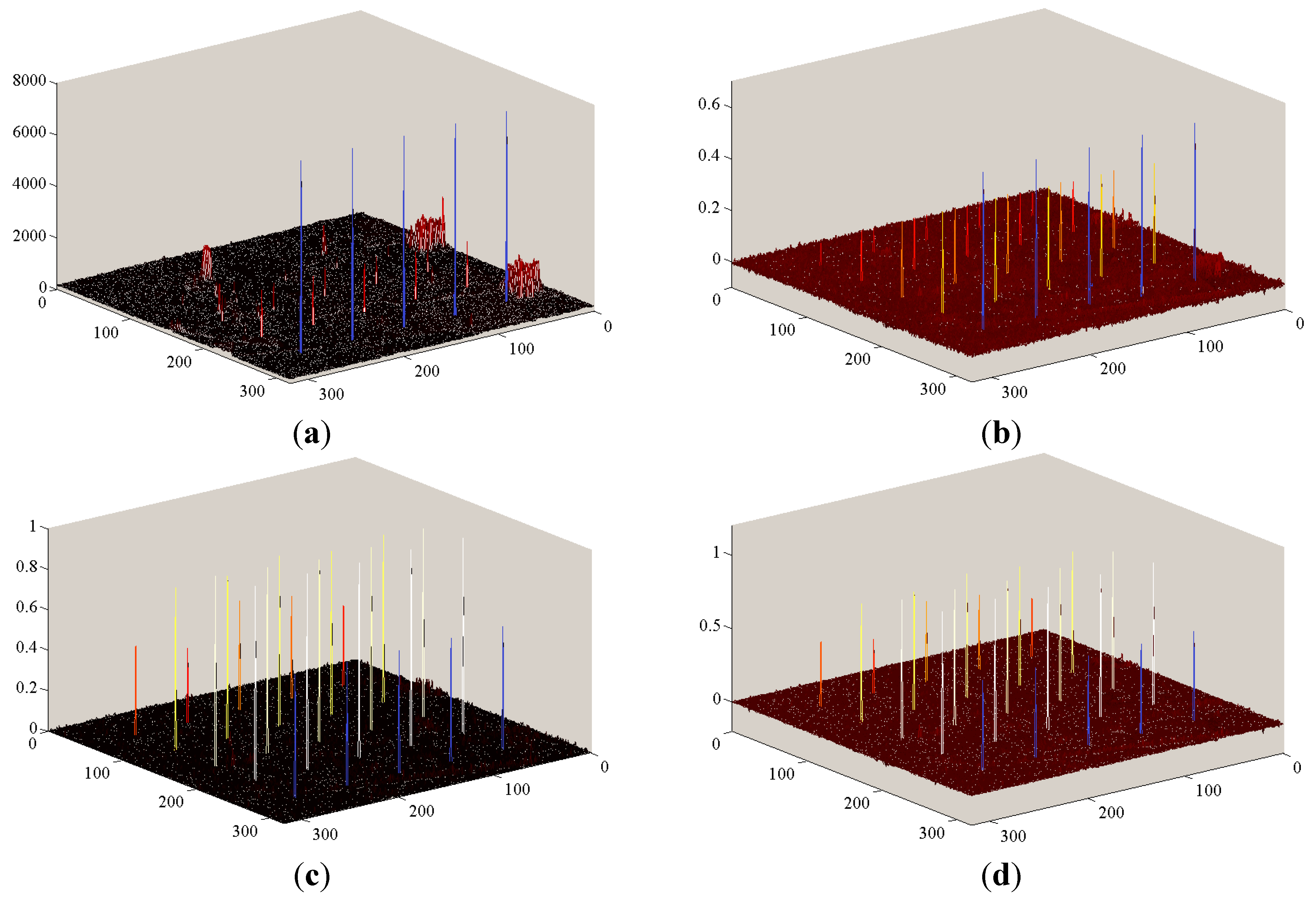
4.1. Experiment Using Data without Strong Non-Target Anomalies

This dataset is a farmland scene in which, the land cover types comprise five main classes, which are, soil, tree, grass, sand, and greenhouses. We chose a mineral named actinolite as the implanted pure target, whose standard spectrum was from the U.S. Geological Survey (USGS) Digital Spectral Library. In order to make it consistent with the AVIRIS data cube, the target spectrum was rescaled to the same range of the image and resampled according to the AVIRIS wavelength.
The target implant method in [39] was used in our work, which is expressed as:
z = f t + ( 1 f ) b
where synthetic spectral signature z with a specified abundance fraction f from a desired target t, contaminated by a background signature b, is simulated. By this method, a 5 × 5 target panel with different implant fraction f from 0.1 to 0.5 is generated. This means that the implanted targets are all sub-pixels. The locations of each target and the implant fractions are shown in Figure 6a, and the spectra of target and five main classes of background are shown in Figure 6b.
Figure 6. (a) Color rendering of the AVIRIS image and implanted target locations. (b) Target spectral signature and background classes have spectral signatures in the AVIRIS dataset.
Remotesensing 07 06611 g006
Furthermore, in order to consider noise effect [40,41], we added additive zero-mean white Gaussian noise to the test dataset. Different noise variances were in different bands, with the signal-to-noise ratio (SNR) being defined as:
SNR dB = 10 log 10 ( σ signal 2 / σ noise 2 )
where σ signal 2 and σ noise 2 are variances of signal and noise components, respectively. Finally, we generate five synthetic test datasets with SNR being10 dB, 15 dB, 20 dB, 25 dB, and 30 dB, respectively. For each synthetic dataset, we employ the following algorithms for comparison: (1) RX; (2) CEM; (3) ACE; (4) the proposed ASMF with n = 1; and (5) the proposed ASMF with n = 2.
ROC curves are also adopted to quantitatively evaluate the detection performance. Figure 7 shows the ROC curves of the detection results, with different SNR values.
It can be seen that, compared to the conventional CEM, our proposed ASMF method improves the detection rate while reducing the false alarm rate (FAR). Further, ASMF with n = 2 produces better performance than n = 1 in all the five tested datasets. In addition, as shown in Figure 7, when the SNR value is more than 25dB, the ROC curve of ACE coincides with the curve of ASMF with n = 1, which means they have similar performance. However, with the increasing of noise level, the ACE algorithm yields more false alarms than both of the ASMF and the CEM. To better demonstrate this point, the FARs under 100% detection [39] for the four algorithms in comparison are shown in Figure 8. In fact, we can see that the FARs of the ASMF with n = 1 is always less than the ACE method, especially in the data with SNR = 10 dB. Figure 9 show the detection output transect plots of row 54 using the four methods on the test datasets with SNR = 10dB. As shown in Figure 6a, there are five implanted targets with 10% implanted fraction in this row. From Figure 9b,c we can see that, although the five target pixels are detected by the ACE and ASMF (n = 1), all the outputs of ACE are positive, while in ASMF, some of them are negative. In most situations, they generate very similar detection performance. However, when the target energy is small, the ACE may lead to more FARs. From Figure 9d, it can be seen that the ASMF with n = 2 maintains target energy and suppresses most other outputs, which offers the best separability between the targets and other non-target pixels.
Figure 7. ROC curves of AVIRIS dataset, when the SNR value of white noise is (a) 30 dB, (b) 25 dB, (c) 20 dB, (d) 15 dB, and (e) 10 dB.
Remotesensing 07 06611 g007
Figure 8. False alarm rate under 100% detection of the synthetic dataset with different degree of white Gaussian noise.
Remotesensing 07 06611 g008
Figure 9. Detection test statistic transect plots of line 54 in synthetic dataset with adding 10 dB white noise. (a) CEM, (b) ACE, (c) ASMF with n = 1, (d) ASMF with n = 2.
Remotesensing 07 06611 g009

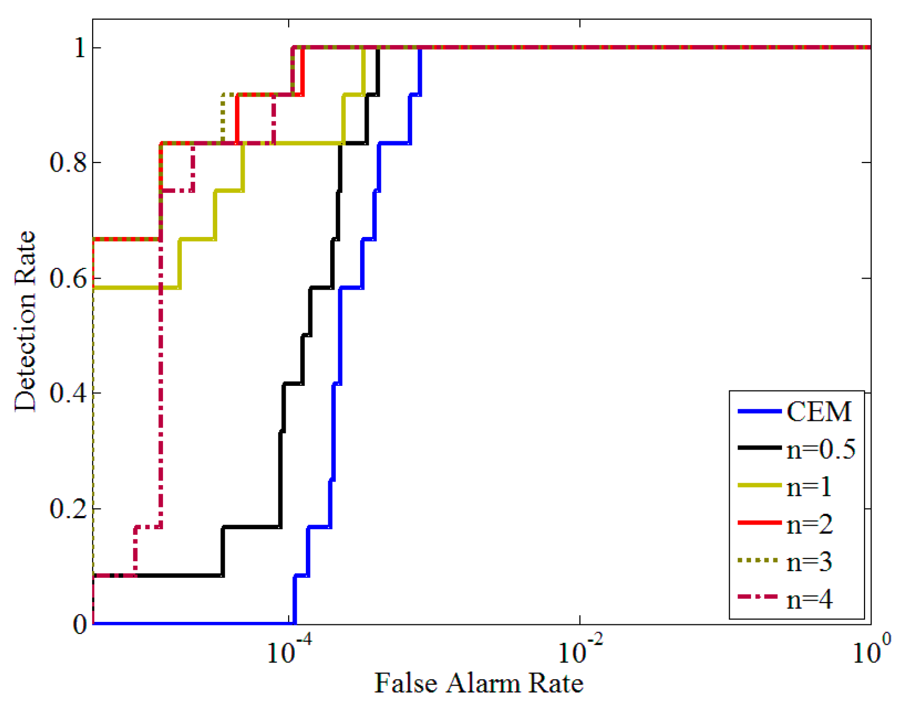
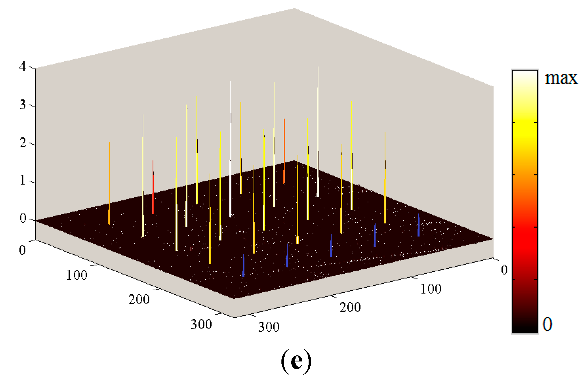
4.2. Experiment Using Data with Strong Non-Target Anomalies

Another synthetic data experiment is arranged to examine detection performance in the situations where there are other undesired anomalies. For this purpose, we implant two kinds of mineral spectra in the AVIRIS dataset, and use one of them as the target. In order to increase the difficulty of detection, we chose two similar spectral signatures but belonging to different minerals. As shown in Figure 10a, the minerals, named nontronite and actinolite, are used in our experiment. Then, we chose the actinolite spectrum as the pure target signature, and the same implant method are used for implanting 20 targets with different implanted fractions from 10% to 40%. While the pure spectral signature of nontronite is implanted as five undesired anomalies laying in a right row of the hyperspectral scene. The detailed locations of both target and anomaly are provided in Figure 10b.
Figure 10. (a) Implanted target and anomaly spectral signatures. (b) Implanted target and anomaly locations.
Remotesensing 07 06611 g010
Figure 11a–e show the 3-D target detection results. From these figures, we can see that the implanted spectral signature of nontronite is detected as apparent anomalies in the output of RX. In the results of CEM algorithm, the five anomaly pixels maintain the largest output, while many targets (implanted fractions are less than 20%) can be hardly observed. The ACE and the ASMF with n = 1 can detect all the 20 targets and suppress anomalies to a lower level, but it is still higher than small abundance targets. Only in the detection result of ASMF with n = 2, all of the outputs of 20 targets are greater than both background and anomalous pixels.
Figure 11. 3-D plots of the detection results for the AVIRIS dataset. (a) RX, (b) CEM, (c) ACE, (d) ASMF n = 1, and (e) ASMF n = 2.
Remotesensing 07 06611 g011aRemotesensing 07 06611 g011b
Here, we again use the detection output of row 54 to illustrate the performance of each algorithm. From Figure 12 we can see that, in this synthetic dataset, the proposed ASMF with n = 2 can detect all the different abundance targets without any false alarm, which shows more effective detection.
Figure 12. Detection results transect plots of line 54. (a) CEM, (b) ACE, (c) ASMF with n = 1, (d) ASMF with n = 2.
Remotesensing 07 06611 g012

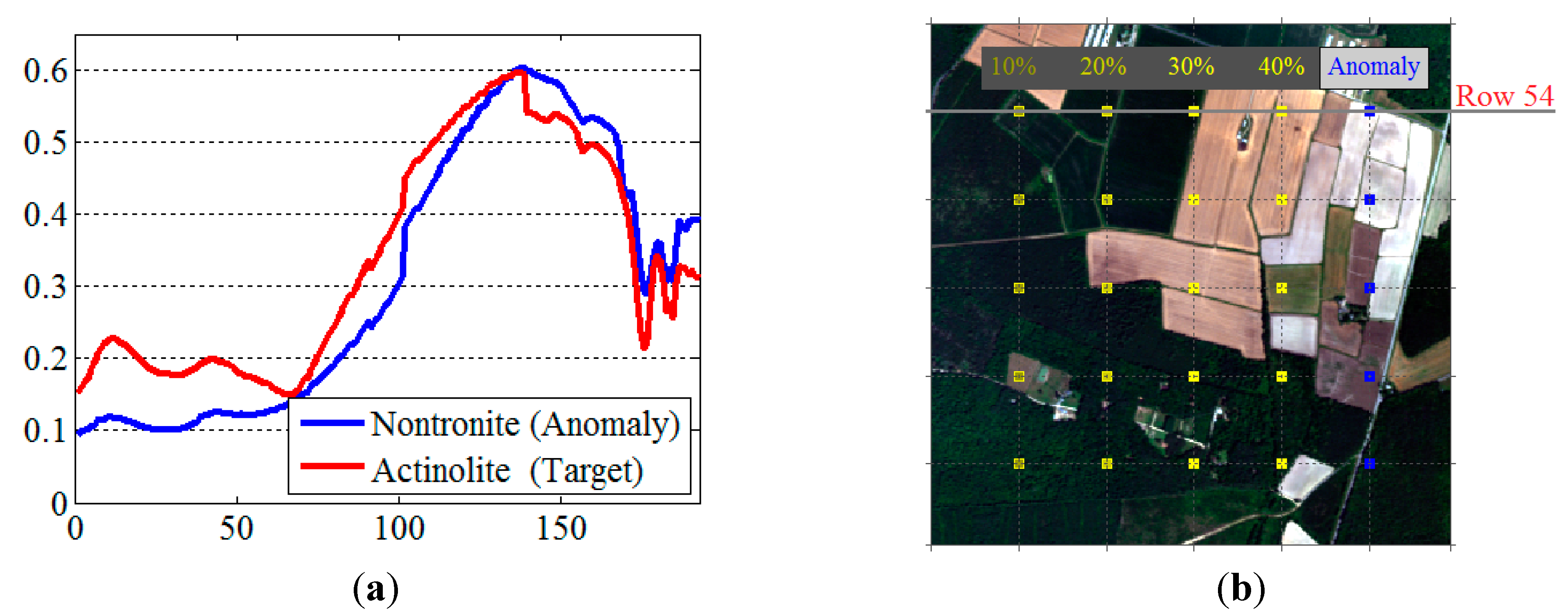
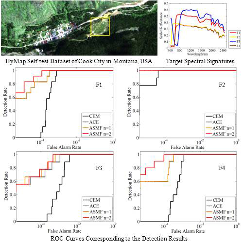
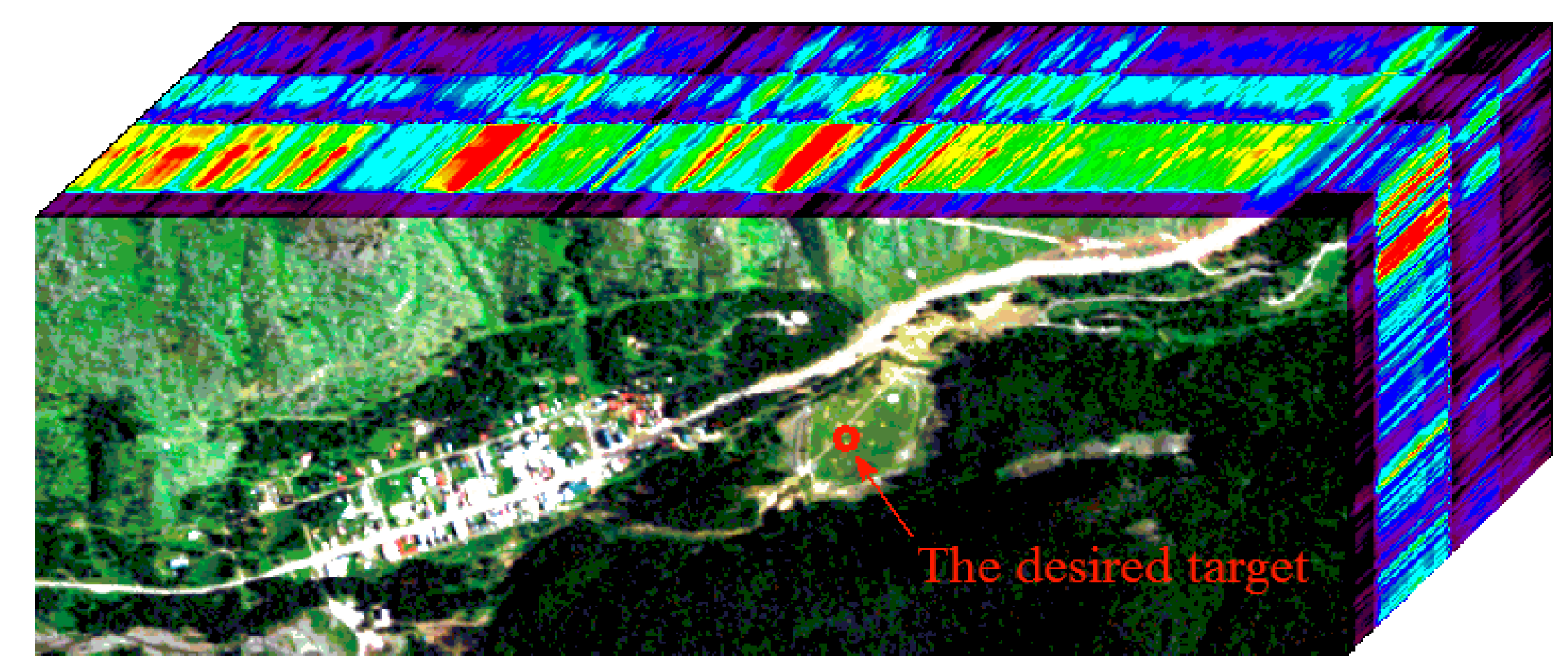
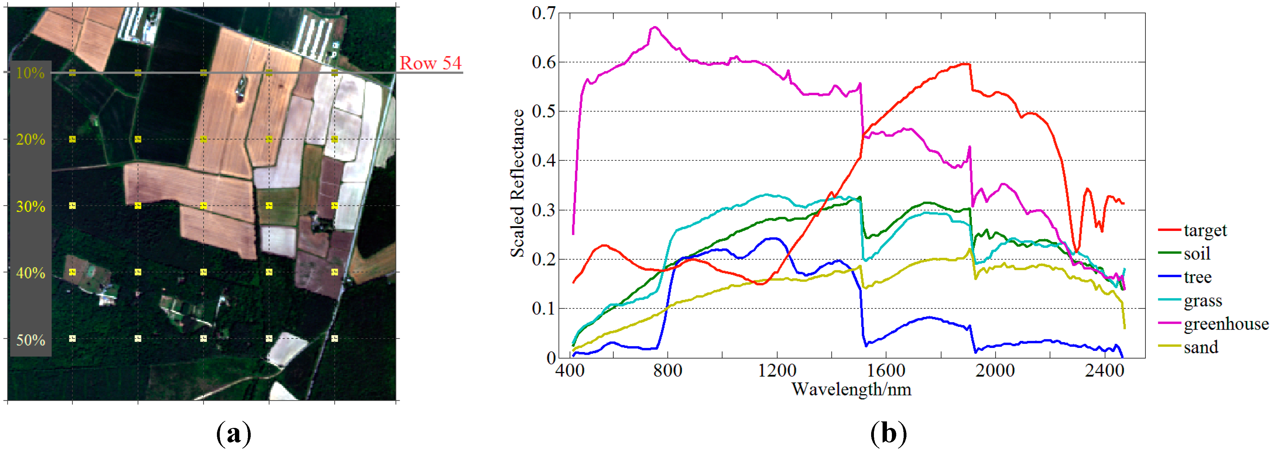
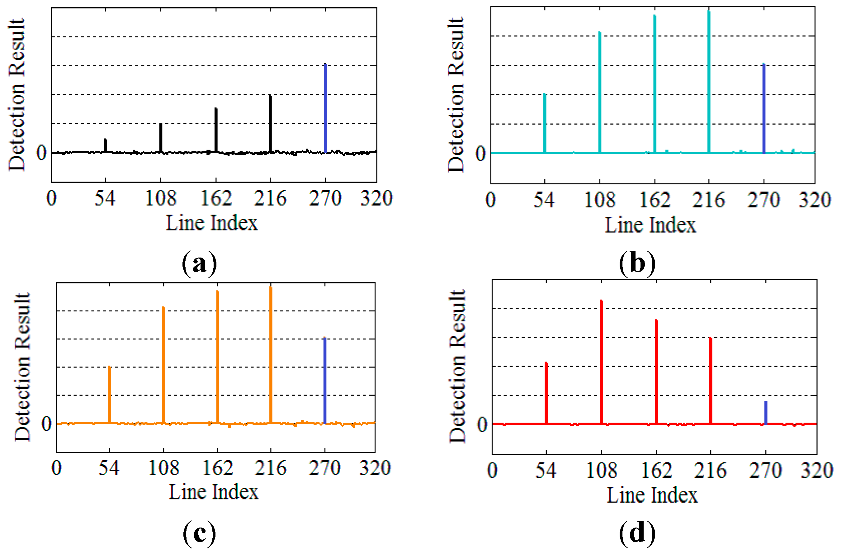
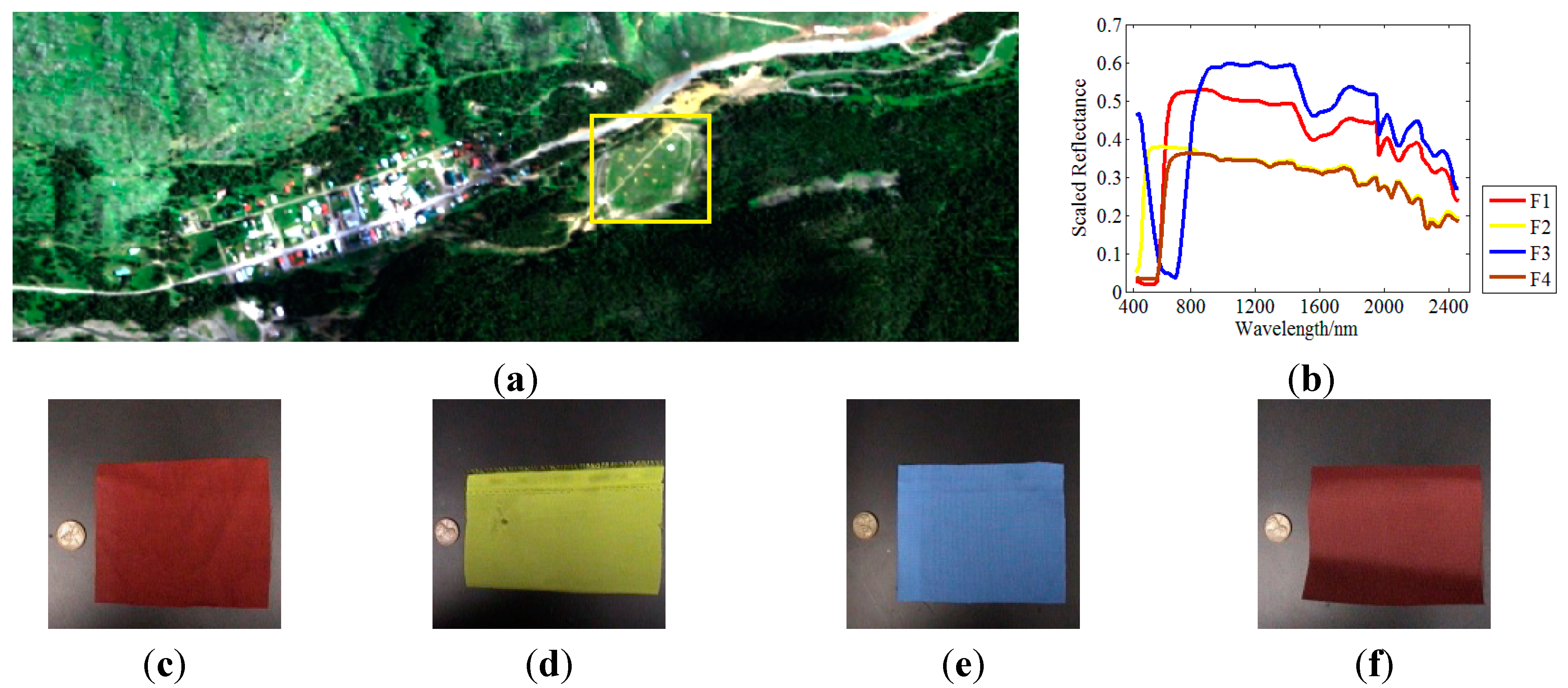
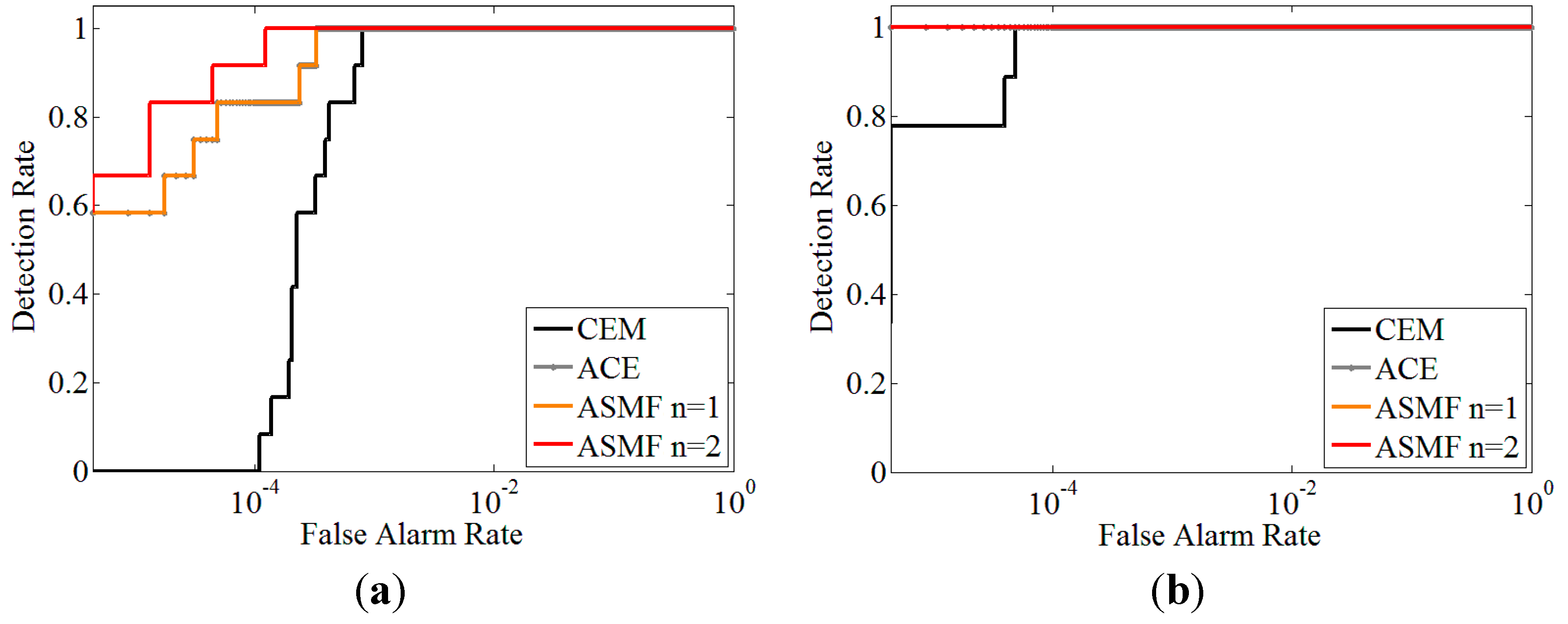
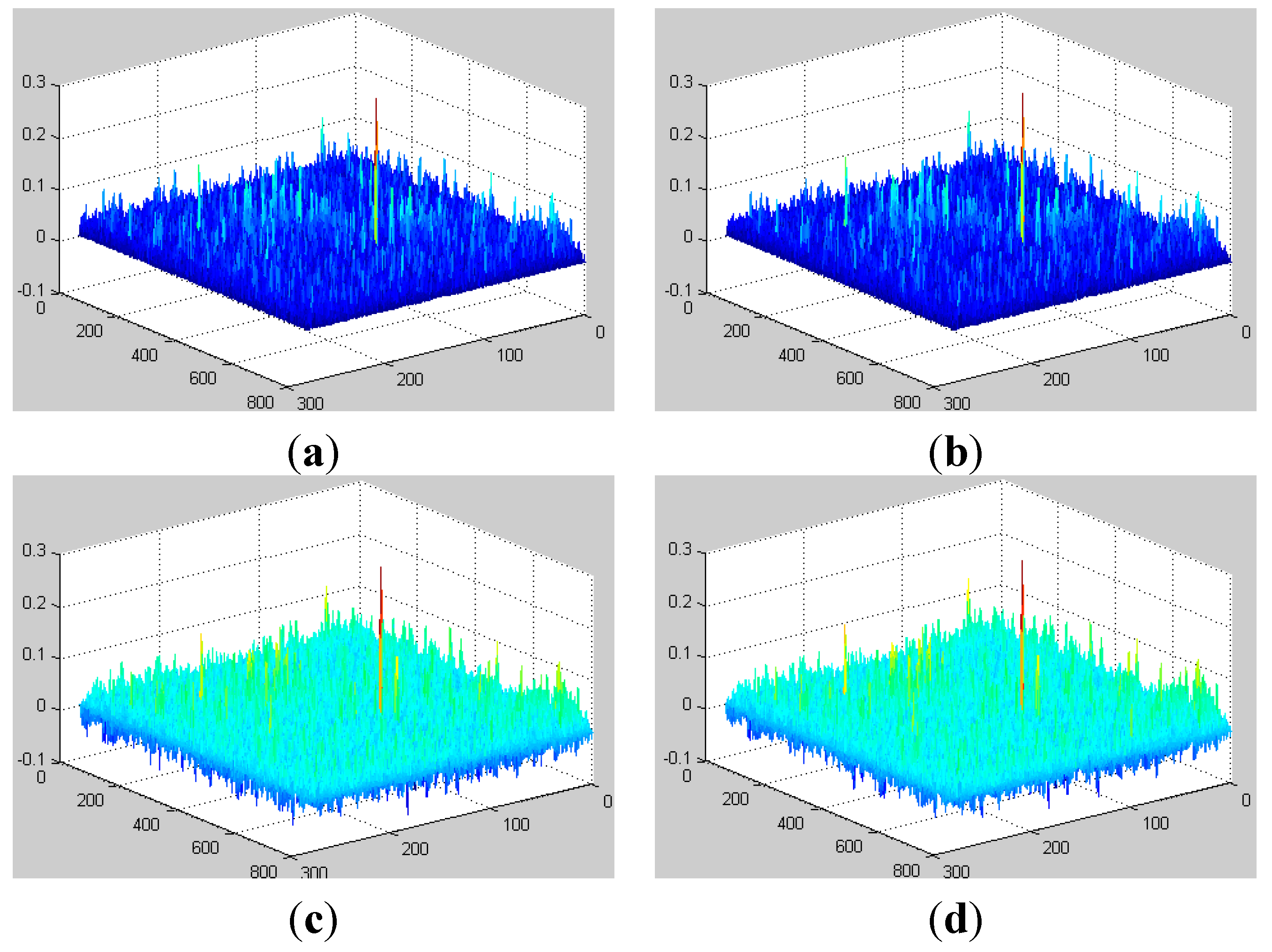
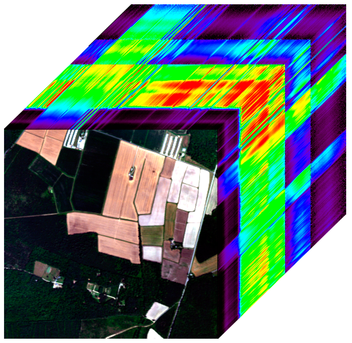
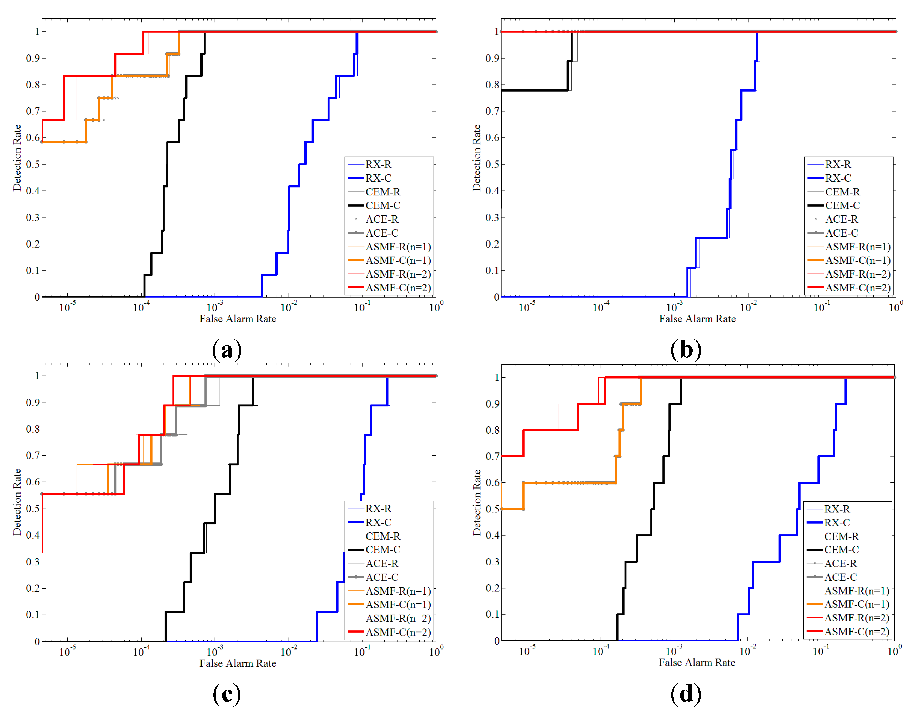
5. Experiments with Real Data

5.1. Experimental Design and Dataset

Real hyperspectral datasets are provided by the Digital Imaging and Remote Sensing Group in Center for Imaging Science at Rochester Institute of Technology. These datasets include a self-test set and a blind-test set, which were successfully applied for performance evaluation in previous studies [42,43,44]. As shown in Figure 1, the datasets include HyMap [45] reflectance images of Cook City in Montana, USA, covering an area of 280 × 800 pixels with 126 spectral bands. The ground resolution of imagery data is approximately 3 m. This dataset is also equipped with the exact locations and standard spectral library (SPL) files of all the test targets, so it is one of the standard datasets for hyperspectral target detection. There is a grass region located in the self-test dataset, as shown in Figure 13a marked by the yellow box. Four real fabric panels (F1–F4) as targets were arranged in this region and details of them are listed in Table 2. The spectrum of each target is obtained and preprocessed by the project-equipped SPL files. By rescaling the SPL spectra to the true reflectance data and re-sampling the SPL spectra according to the sensor wavelength, we obtain the prior target spectra for detection, as shown in Figure 13b. Figure 13c–f illustrate the ground truth image including different targets.
Table 2. Characteristics of real targets.
NameSizeType
F13 × 3 mRed Cotton
F23 × 3 mYellow Nylon
F3a2 × 2 mBlue Cotton
F3b1 × 1 mBlue Cotton
F4a2 × 2 mRed Nylon
F4b1 × 1 mRed Nylon
Figure 13. (a) RGB composites of the HyMap self-test dataset with the location of the grass region. (b) Four target spectral signatures. (cf) Ground truth photos of targets F1, F2, F3, and F4, respectively.
Remotesensing 07 06611 g013
Before starting the experiments, we use the RX algorithm to simply view the distribution of potential anomalies in this dataset. As shown in Figure 14, there are abundant anomalies existing in the city region, which are distinct from natural background. In contrast, the grass region where the targets are present shows few abnormal points. For this reason, both local and global images are used to evaluate our algorithm. Since all the targets were located in the open grass region, the portion of 90 × 90 pixels was chosen as the local image which covers the entire open grass region (see Figure 13a). For the global image, the whole hyperspectral dataset is used, which includes heterogeneous background increasing the difficulty of target detection.
Figure 14. 2-D plots of the detection results of the RX algorithm.
Remotesensing 07 06611 g014

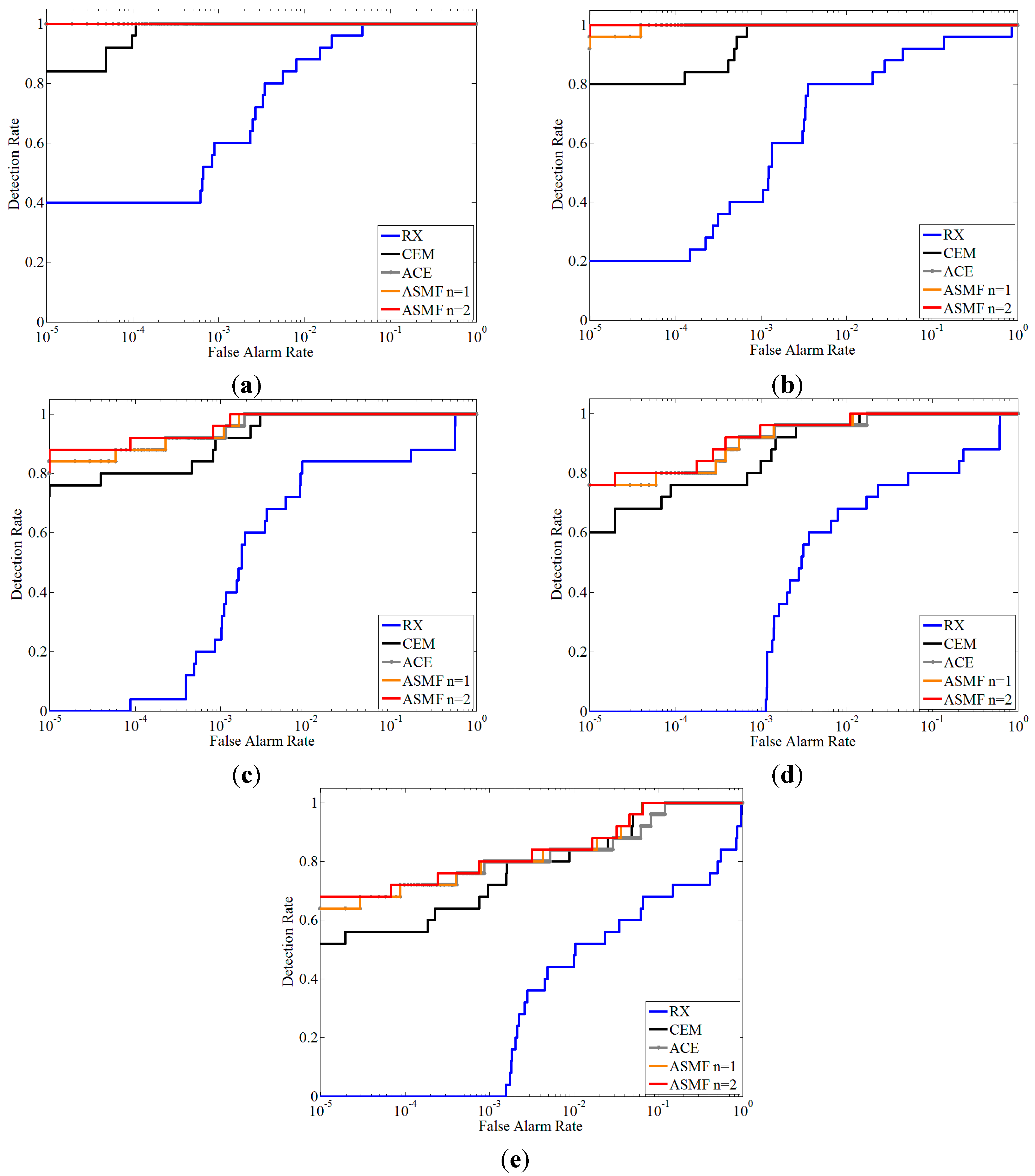
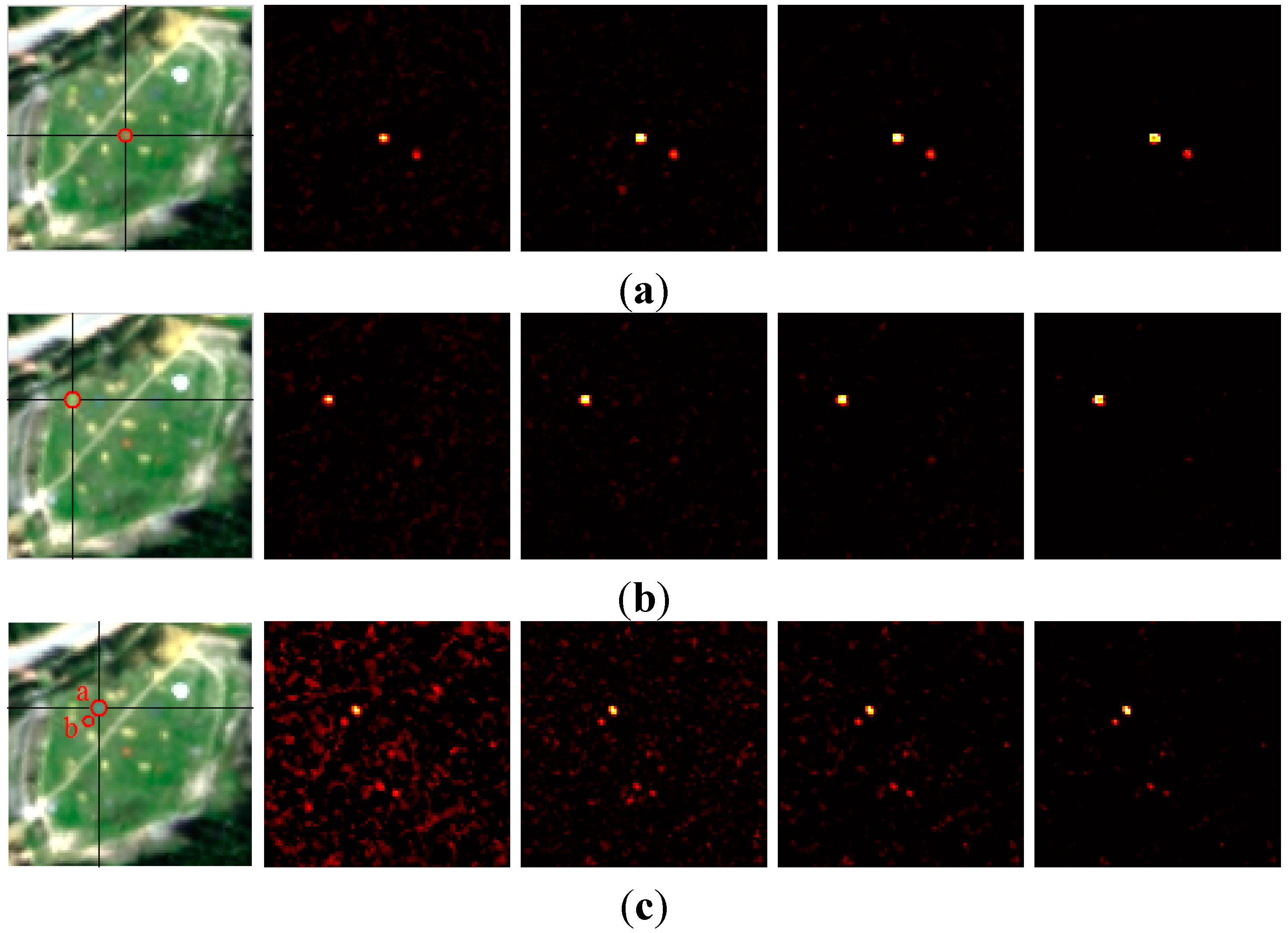
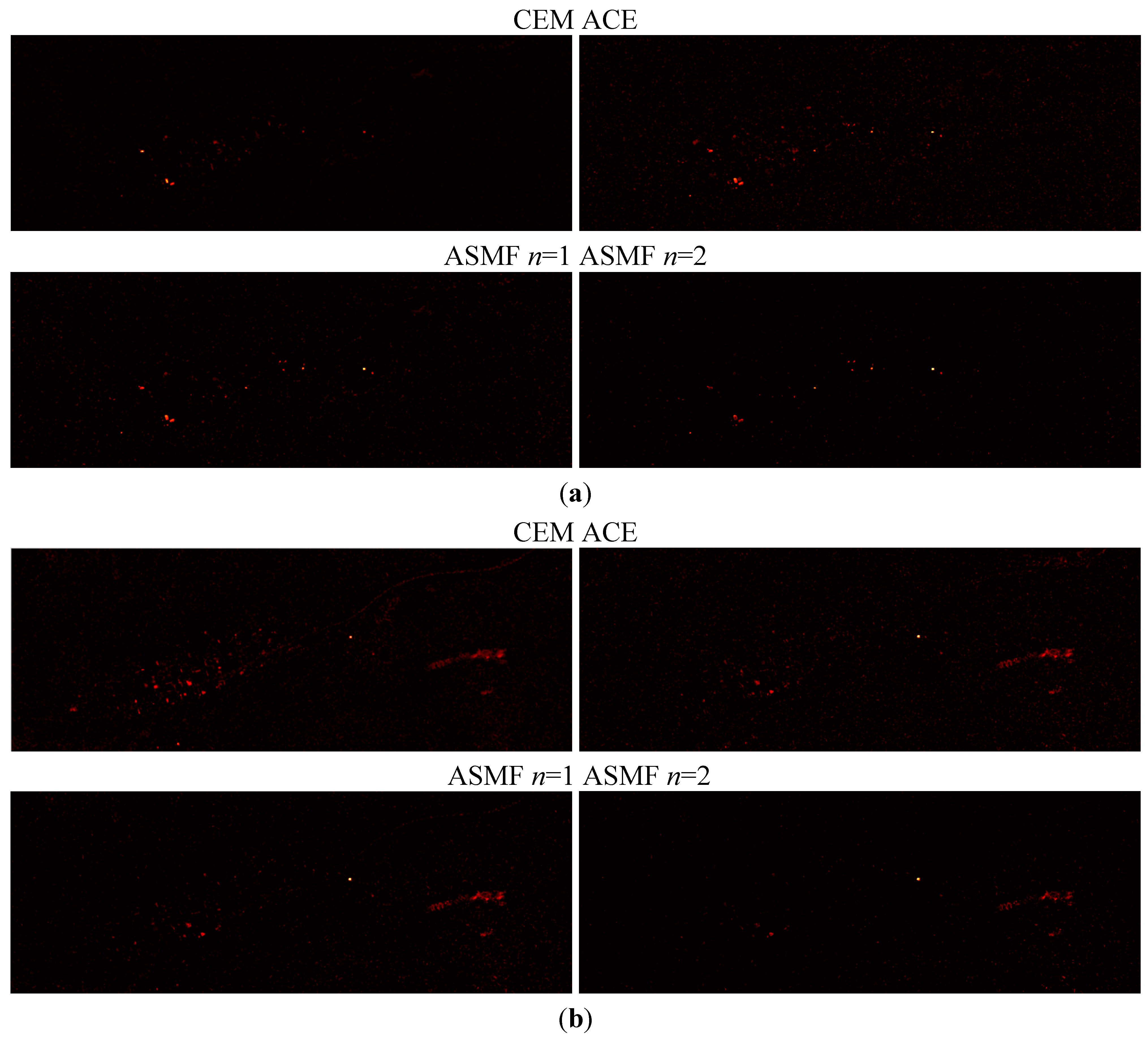
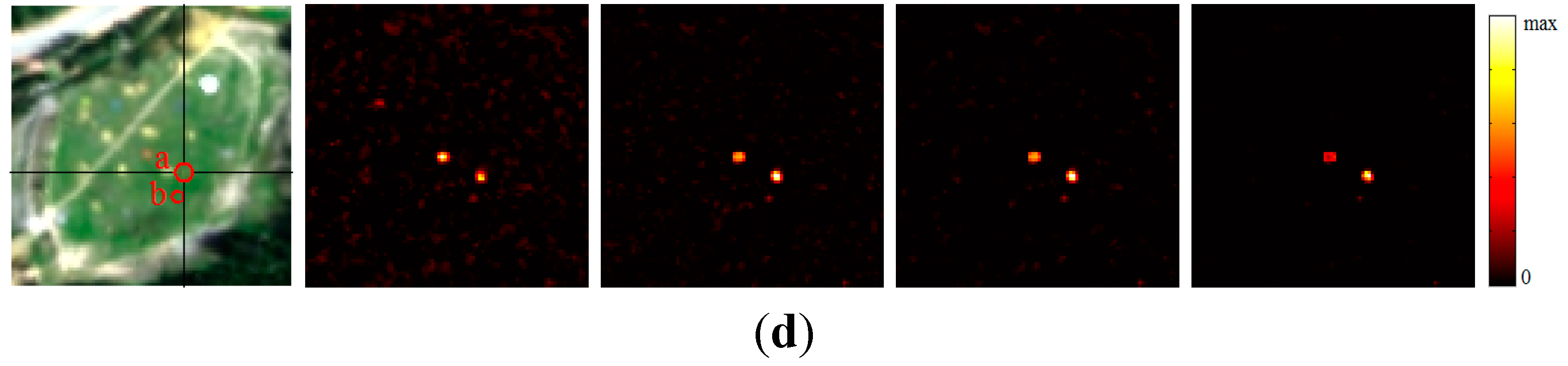
5.2. Experiment Using a Local Image with Homogeneous Background

In the experiment using the local image, the background is relative homogeneous. The detection results are reported in Figure 15. The left column lists the locations of F1–F4 in this grass region, then, the 2-D plots of the detection results of CEM, ACE, ASMF with n = 1, and ASMF with n = 2 are shown from left to right, respectively. In order to show the detection results more clearly, all the 2-D plots are simply linearly enhanced from 0 to the max. We can observe that all the compared algorithms can detect the targets. The difference is that the proposed ASMF method provided brighter target pixels and less isolated pixels as false alarms, especially when n = 2. For quantitative evaluation purposes, Figure 16 presents the ROC curves corresponding to the detection results reported in Figure 15. Further, we compare the target detection FARs under 100% detection of the four algorithms in Table 3. In the detection of target F2, all the algorithms detected the target effectively with no false alarm. In the detection of target F1, F3 and F4, these curves and the FAR scores reveal that our proposed ASMF offers a lower FAR, which is more superior to the conventional CEM algorithm. It should be pointed out that, in this considered dataset, the ACE and ASMF with n = 1 exhibit the same detection performance.
Figure 15. Locations and detection results obtained by the compared algorithms of (a) F1, (b) F2, (c) F3, and (d) F4, where results of CEM, ACE, ASMF with n = 1, and ASMF with n = 2 are shown from left to right in each row.
Remotesensing 07 06611 g015aRemotesensing 07 06611 g015b
Figure 16. ROC curves corresponding to the detection results reported in Figure 15. (a) F1, (b) F2, (c) F3, and (d) F4.
Remotesensing 07 06611 g016
Table 3. FARs under 100% detection.
AlgorithmsCEMACEASMF n = 1ASMF n = 2
F14.95 × 10−46.18 × 10−46.18 × 10−42.47 × 10⁻⁴
F20000
F31.24 × 10−4000
F42.30 × 10−32.00 × 10−32.00 × 10−32.00 × 10⁻³

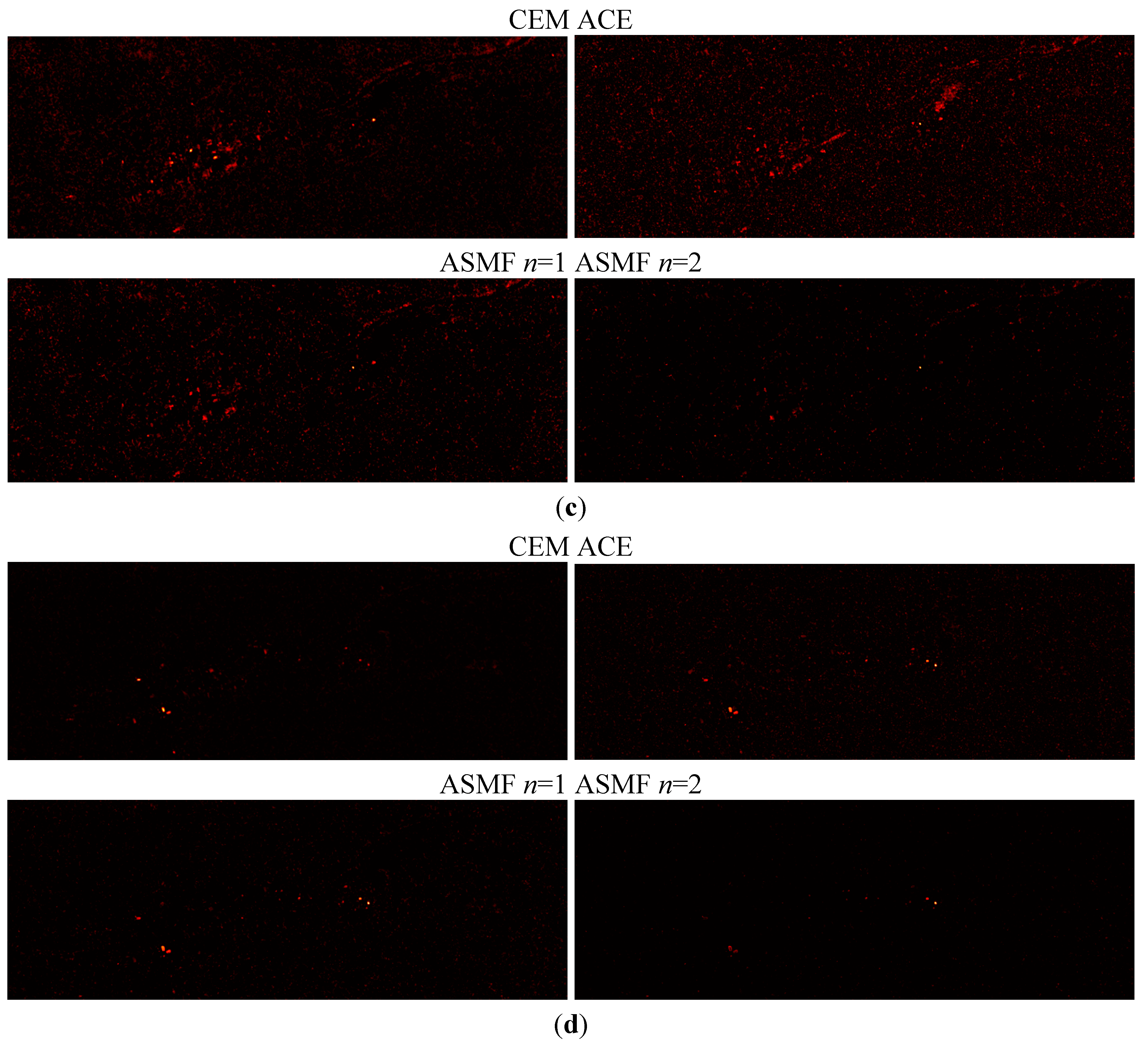
5.3. Experiment Using the Entire Image with Heterogeneous Background
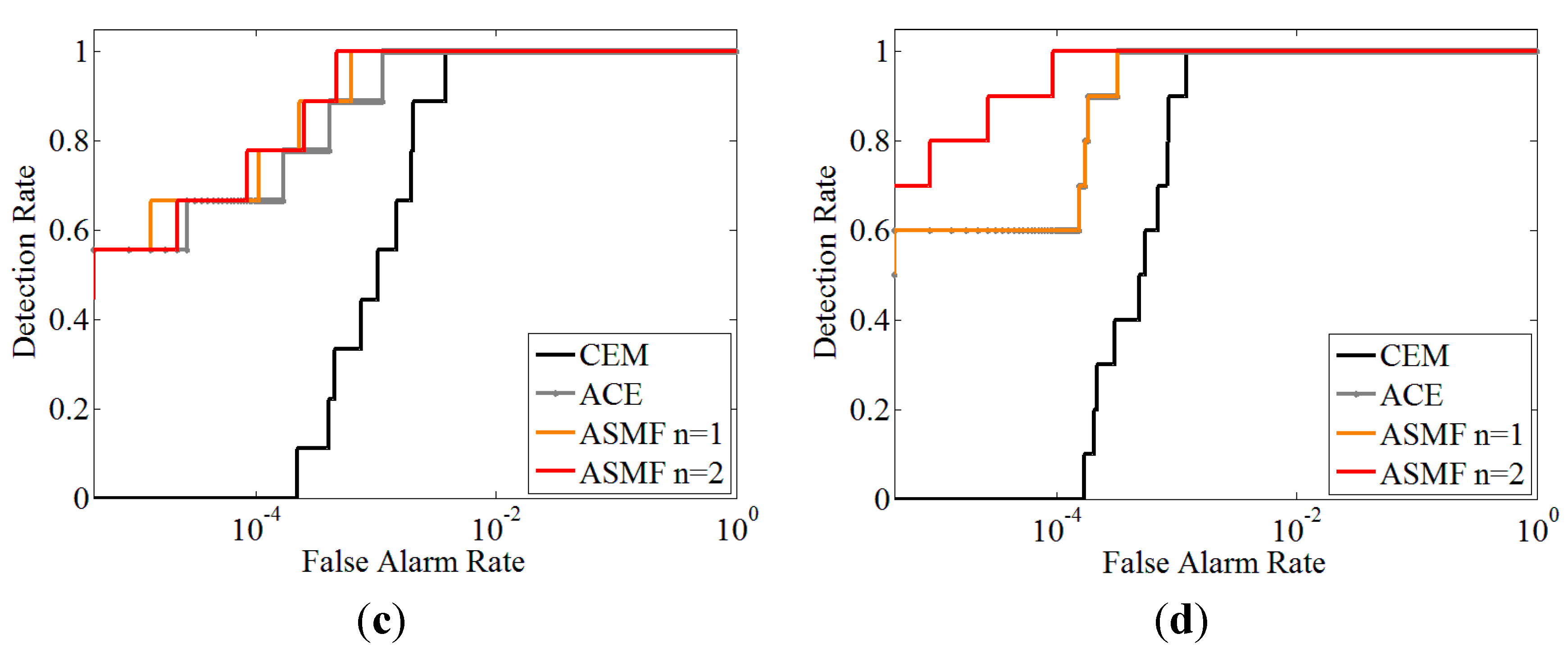
In the experiment of using the global image, the 2-D plots of the detection results of all the compared algorithms for different targets are shown in Figure 17a–d. Obviously, the added pixels, especially the abnormal pixels in the city region, greatly interrupt target detection. In the outputs of the CEM, the brightest pixels are distributed in the city region (as shown in the detection of F1, F3 and F4), which are conspicuous false alarms. By using our proposed ASMF method, the false alarms are partly suppressed while the real targets are enhanced. In particular, the ASMF with n = 2 produces the fewest false alarms and the largest target outputs.
Based on these detection results, the ROC curves are shown in Figure 18, and Table 4 lists the FARs by each algorithm under 100% detection rate. In the comparison, we can see that our proposed ASMF method greatly improved the detection performance. In the detection of F1, F2, and F4, ASMF with n = 1 has the same performance as ACE and is better than CEM. However, in the detection of F3, the ASMF with n = 1 performs more excellently than ACE. In this work, the ASMF with n = 2 generates the best performance. As shown in Table 4, it is remarkable that the proposed ASMF with n = 2 provided the lowest FAR than other compared methods.
Figure 17. 2-D plots of the detection results using the whole HyMap dataset by all the comparison algorithms of (a) F1, (b) F2, (c) F3, and (d) F4.
Remotesensing 07 06611 g017aRemotesensing 07 06611 g017b
Figure 18. ROC curves corresponding to Figure 17 of (a) F1, (b) F2, (c) F3, and (d) F4.
Remotesensing 07 06611 g018aRemotesensing 07 06611 g018b
Table 4. FARs under 100% detection.
AlgorithmsCEMACEASMF n = 1ASMF n = 2
F18.08 × 10−43.3 × 10−43.3 × 10−41.25 × 10⁻⁴
F24.91 × 10−5000
F33.83 × 10−31.14 × 10−36.29 × 10−44.69 × 10⁻⁴
F41.20 × 10−33.21 × 10−43.21 × 10−49.38 × 10⁻⁵
In summary, the experiments conducted using both local and global real datasets indicate satisfactory performance of the proposed ASMF method. Although the original CEM algorithm can detect targets effectively in many circumstances, the ASMF can be more adaptive in a complex environment where there exist strong abnormal pixels. We believe that the ASMF is a simple yet powerful method to improve the original target detection performance.

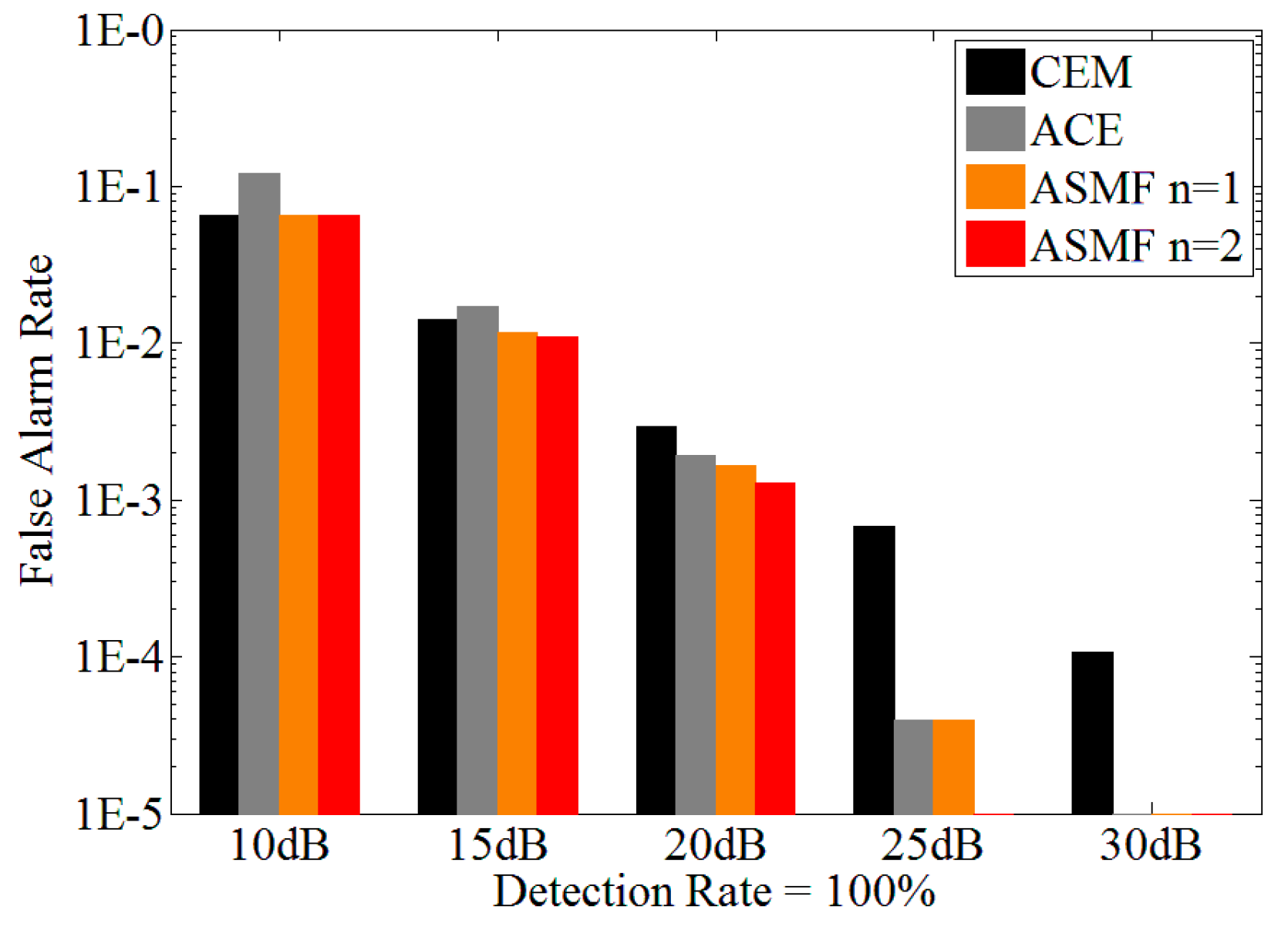
5.4. Analysis of Using Covariance Matrix

All the algorithms can be implemented using the covariance matrix. Thus, in this subsection, we further investigate the performance difference between the algorithms with the covariance matrix. The ROC curves are shown in Figure 19, where the correlation-based algorithms (RX-R, CEM-R, ACE-R and ASMF-R) marked by the thin lines are compared to the standard covariance-based algorithms (RX-C, CEM-C, ACE-C and ASMF-C) marked by the thick lines.
We can see that, in the detection of target F1–F3 (Figure 19a–c), the results of covariance-based algorithms are slightly better than those algorithms with correlation matrix, but in the detection of target F4 (Figure 19d), the situation is reversed. In fact, these two kinds of algorithms have similar detection performance in our experiments, and both of them are improved by the proposed ASMF method, especially when n = 2. It is worth mentioning that, although in most situations the ROC curve of ASMF with n = 1 coincides with the curve of ACE (using correlation or covariance matrix), it offers better performance than ACE in the detection of target F3, as shown in Figure 19c. For clearer demonstration, the 3-D detection results of target F3 by ASMF with n = 1 and ACE are shown in Figure 20. Obviously, the performance improvement is owed to keeping the sign of the detection results.
Figure 19. ROC curves of the HyMap real hyperspectral datasets according to the correlation-based and covariance-based algorithms when the target is (a) F1, (b) F2, (c) F3, and (d) F4.
Remotesensing 07 06611 g019
Figure 20. 3-D plots of the detection results of target F3. (a) ACE-R; (b) ACE-C; (c) ASMF-R (n = 1); (d) ASMF-C (n = 2).
Remotesensing 07 06611 g020

6. Conclusions

In this paper, we presented a novel ASMF method based on the combination of supervised target detection and anomaly detection. A typical case was demonstrated by fusing CEM and RX algorithms, in which, RX detection result was used to adjust the output of CEM. Meanwhile, to pursue the effective adjustment and avoid over-amplification of background signals, a tunable factor was arranged to control the strength of the adjustment. Experimental results on synthetic and real data show that the proposed method significantly improved the target detection precision in comparison with the original method.

Acknowledgments

The authors would like to thank the Digital Imaging and Remote Sensing Group, Center for Imaging Science, Rochester Institute of Technology, for providing the HyMap datasets used in our experiments. This research was supported by the Key Research Program of the Chinese Academy of Sciences under Grant No. KZZD-EW-TZ-18, and by the National Natural Science Foundation of China under Grant No. 41325004.

Author Contributions

Lianru Gao mainly was responsible for mathematics modeling, experiments designing, and structure organizing. Bin Yang finished most of the experimental and analytical works. Qian Du helped to complete the theoretical framework and improve the quality of the paper. Bing Zhang provided the original ideas on the proposed method.

Conflicts of Interest

The authors declare no conflict of interest.

References

  1. Goetz, A.F.; Vane, G.; Solomon, J.E.; Rock, B.N. Imaging spectrometry for Earth remote sensing. Science 1985, 228, 1147–1153. [Google Scholar] [CrossRef] [PubMed]
  2. Manolakis, D.; Shaw, G. Detection algorithms for hyperspectral imaging applications. IEEE Signal. Proc. Mag. 2002, 19, 29–43. [Google Scholar] [CrossRef]
  3. Kerekes, J.P.; Baum, J.E. Spectral imaging system analytical model for subpixel object detection. IEEE Trans. Geosci. Remote Sens. 2002, 40, 1088–1101. [Google Scholar] [CrossRef]
  4. Plaza, A.; Benediktsson, J.A.; Boardman, J.; Brazile, J.; Bruzzone, L.; Camps-Valls, G.; Chanussot, J.; Fauvel, M.; Gamba, P.; Gualtieri, J.; et al. Recent advances in techniques for hyperspectral image processing. Remote Sens. Environ. 2009, 113, 110–122. [Google Scholar] [CrossRef]
  5. Fauvel, M.; Tarabalka, Y.; Benediktsson, J.A.; Chanussot, J.; Tilton, J.C. Advances in spectral-spatial classification of hyperspectral images. Proc. IEEE 2013, 101, 652–675. [Google Scholar] [CrossRef]
  6. Bioucas-Dias, J.M.; Plaza, A.; Camps-Valls, G.; Scheunders, P.; Nasrabadi, N.M.; Chanussot, J. Hyperspectral remote sensing data analysis and future challenges. IEEE Geosci. Remote Sens. Mag. 2013, 1, 6–36. [Google Scholar] [CrossRef]
  7. Nasrabadi, N.M. Hyperspectral target detection: An overview of current and future challenges. IEEE Signal Process. Mag. 2014, 31, 34–44. [Google Scholar] [CrossRef]
  8. Eismann, M.T.; Stocker, A.D.; Nasrabadi, N.M. Automated hyperspectral cueing for civilian search and rescue. Proc. IEEE 2009, 97, 1031–1055. [Google Scholar] [CrossRef]
  9. Averbuch, A.; Zheludev, M. Two linear unmixing algorithms to recognize targets using supervised classification and orthogonal rotation in airborne hyperspectral images. Remote Sens. 2012, 4, 532–560. [Google Scholar] [CrossRef]
  10. Scharf, L.L.; Friedlander, B. Matched subspace detectors. IEEE Trans. Signal Process. 1994, 42, 2146–2157. [Google Scholar] [CrossRef]
  11. Robey, F.C.; Fuhrmann, D.R.; Kelly, E.J. A CFAR adaptive matchedfilter detector. IEEE Trans. Aerosp. Electron. Syst. 1992, 28, 208–216. [Google Scholar] [CrossRef]
  12. Chang, C.I.; Ren, H.; Chiang, S.S. Real-time processing algorithms for target detection and classification in hyperspectral imagery. IEEE Trans. Geosci. Remote Sens. 2001, 39, 760–768. [Google Scholar] [CrossRef]
  13. Du, Q.; Nekovei, R. Fast real-time onboard processing of hyperspectral imagery for detection and classification. J. Real-Time Image Process. 2009, 4, 273–286. [Google Scholar] [CrossRef]
  14. Harsanyi, J.C.; Chang, C.I. Hyperspectral image classification and dimensionality reduction: An orthogonal subspace projection approach. IEEE Trans. Geosci. Remote Sens. 1994, 32, 779–785. [Google Scholar] [CrossRef]
  15. Chang, C.I. Orthogonal subspace projection (OSP) revisited: A comprehensive study and analysis. IEEE Trans. Geosci. Remote Sens. 2005, 43, 502–518. [Google Scholar] [CrossRef]
  16. Kelly, E.J. An adaptive detection algorithm. IEEE Trans. Aerosp. Electron. Syst. 1986, AES-22, 115–127. [Google Scholar] [CrossRef]
  17. Chen, Y.; Nasrabadi, N.M.; Tran, T.D. Effects of linear projections on the performance of target detection and classification in hyperspectral imagery. J. Appl. Remote Sens. 2011, 5. [Google Scholar] [CrossRef]
  18. Du, Q.; Chang, C.-I. A signal-decomposed and interference-annihilated approach to hyperspectral target detection. IEEE Trans. Geosci. Remote Sens. 2004, 42, 892–906. [Google Scholar]
  19. Banerjee, A.; Burlina, P.; Diehl, C. A support vector method for anomaly detection in hyperspectral imagery. IEEE Trans. Geosci. Remote Sens. 2006, 44, 2282–2291. [Google Scholar] [CrossRef]
  20. Kwon, H.; Nasrabadi, N.M. A comparative analysis of kernel subspace target detectors for hyperspectral imagery. EURASIP J. Adv. Signal Process. 2007, 2007. [Google Scholar] [CrossRef]
  21. Reed, S.; Yu, X. Adaptive multiple-band CFAR detection of an optical pattern with unknown spectral distribution. IEEE Trans. Acoust. Speech Signal Process. 1990, 38, 1760–1770. [Google Scholar] [CrossRef]
  22. Matteoli, S.; Diani, M.; Corsini, G. A tutorial overview of anomaly detection in hyperspectral images. IEEE Aerosp. Electron. Syst. Mag. 2010, 25, 5–27. [Google Scholar] [CrossRef]
  23. Stein, D.W.J.; Beaven, S.G.; Hoff, L.E.; Winter, E.M.; Schaum, A.P.; Stocker, A.D. Anomaly detection from hyperspectral imagery. IEEE Signal Process. Mag. 2002, 19, 58–69. [Google Scholar] [CrossRef]
  24. Schaum, A. Joint subspace detection of hyperspectral targets. In Proceeding of 2004 IEEE Aerospace Conference Proceedings, Big Sky, MT, USA, 6–13 March 2004; Volume 3, pp. 1818–1824.
  25. Schaum, A. Hyperspectral anomaly detection beyond RX. Proc. SPIE 2007, 6565. [Google Scholar] [CrossRef]
  26. Matteoli, S.; Diani, M.; Corsini, G. Different approaches for improved covariance matrix estimation in hyperspectral anomaly detection. In Proceedings of the Annual Meeting of the Italian National Telecommunications and Information Theory Group (GTTI’09), Parma, Italy, 23–25 June 2009; pp. 1–8.
  27. Hansen, P.C. Rank-Deficient and Discrete III-Posed Problems: Numerical Aspects of Linear Inversion; Society for Industrial and Applied Mathematics: Philadelphia, PA, USA, 1998. [Google Scholar]
  28. Goldberg, H.; Nasrabadi, N.M. A comparative study of linear and nonlinear anomaly detectors for hyperspectral imagery. Proc. SPIE 2007, 6565. [Google Scholar] [CrossRef]
  29. Kwon, H.; Nasrabadi, N.M. Kernel RX-algorithm: A nonlinear anomaly detector for hyperspectral imagery. IEEE Trans. Geosci. Remote Sens. 2005, 43, 388–397. [Google Scholar] [CrossRef]
  30. Manolakis, D.; Siracusa, C.; Shaw, G. Hyperspectral subpixel target detection using the linear mixing model. IEEE Trans. Geosci. Remote Sens. 2001, 39, 1392–1409. [Google Scholar] [CrossRef]
  31. Du, Q.; Kopriva, I. Automated target detection and discrimination using constrained kurtosis maximization. IEEE Geosci. Remote Sens. Lett. 2008, 5, 38–42. [Google Scholar] [CrossRef]
  32. Chang, C.I.; Chiang, S.S. Anomaly detection and classification for hyperspectral imagery. IEEE Trans. Geosci. Remote Sens. 2002, 40, 1314–1325. [Google Scholar] [CrossRef]
  33. Scharf, L.L.; McWhorter, L.T. Adaptive matched subspace detectors and adaptive coherence estimators. In Proceedings of the Thirtieth Asilomar Conference on Signals, Systems and Computers, Pacific Grove, CA, USA, 3–6 November 1996; Volume 2, pp. 1114–1117.
  34. Zhang, L.; Du, B.; Zhong, Y. Hybrid detectors based on selective endmembers. IEEE Trans. Geosci. Remote Sens. 2010, 48, 2633–2646. [Google Scholar] [CrossRef]
  35. Matteoli, S.; Acito, N.; Diani, M.; Corsini, G. An automatic approach to adaptive local background estimation and suppression in hyperspectral target detection. IEEE Trans. Geosci. Remote Sens. 2011, 49, 790–899. [Google Scholar]
  36. Snyder, D.; Kerekes, J.; Fairweather, I.; Crabtree, R.; Shive, J.; Hager, S. Development of a web-based application to evaluate target finding algorithms. In Proceedings of IEEE International Geoscience and Remote Sensing Symposium (IGARSS), Boston, MA, USA, 7–11 July 2008; Volume 2, pp. 915–918.
  37. Eismann, M.T. Hyperspectral Remote Sensing; SPIE Press: Washington, DC, USA, 2012; pp. 620–624. [Google Scholar]
  38. Green, R.O.; Eastwood, M.L.; Sarture, C.M.; Chrien, T.G.; Aronsson, M.; Chippendale, B.J.; Faust, J.A.; Pavri, B.E.; Chovit, C.J.; Solis, M.; Olah, M.R.; Williams, O. Imaging spectroscopy and the Airborne Visible/Infrared Imaging Spectrometer (AVIRIS). Remote Sens. Environ. 1998, 65, 227–248. [Google Scholar] [CrossRef]
  39. Stefanou, M.S.; Kerekes, J.P. A method for assessing spectral image utility. IEEE Trans. Geosci. Remote Sens. 2009, 47, 1698–1706. [Google Scholar] [CrossRef]
  40. Chen, G.; Qian, S.E. Denoising of hyperspectral imagery using principal component analysis and wavelet shrinkage. IEEE Trans. Geosci. Remote Sens. 2011, 49, 973–980. [Google Scholar] [CrossRef]
  41. Zhang, L.; Zhang, L.; Tao, D.; Huang, X. Sparse transfer manifold embedding for hyperspectral target detection. IEEE Trans. Geosci. Remote Sens. 2014, 52, 1030–1043. [Google Scholar] [CrossRef]
  42. Zhang, L.; Zhang, L.; Tao, D.; Huang, X.; Du, B. Hyperspectral remote sensing image subpixel target detection based on supervised metric learning. IEEE Trans. Geosci. Remote Sens. 2014, 52, 4955–4965. [Google Scholar] [CrossRef]
  43. Khazai, S.; Homayouni, S.; Safari, A.; Mojaradi, B. Anomaly detection in hyperspectral images based on an adaptive support vector method. IEEE Geosci. Remote Sens. Lett. 2011, 8, 646–650. [Google Scholar] [CrossRef]
  44. Khazai, S.; Safari, A.; mojaradi, B.; Homayouni, S. An approach for subpixel anomaly detection in hyperspectral images. IEEE J. Sel. Top. Appl. Earth Obs. Remote Sens. 2013, 6, 769–778. [Google Scholar] [CrossRef]
  45. Cocks, T.; Jenssen, R.; Stewart, A.; Wilson, I.; Shields, T. The HyMap airborne hyperspectral sensor: The system, calibration and performance. In Proceedings of 1st EARSEL Workshop on Imaging Spectroscopy, Zurich, Switzerland, October 1998; pp. 37–42.

