
A Revised Temporal Scaling Method to Yield Better ET Estimates at a Regional Scale


Abstract
:
1. Introduction
2. Data
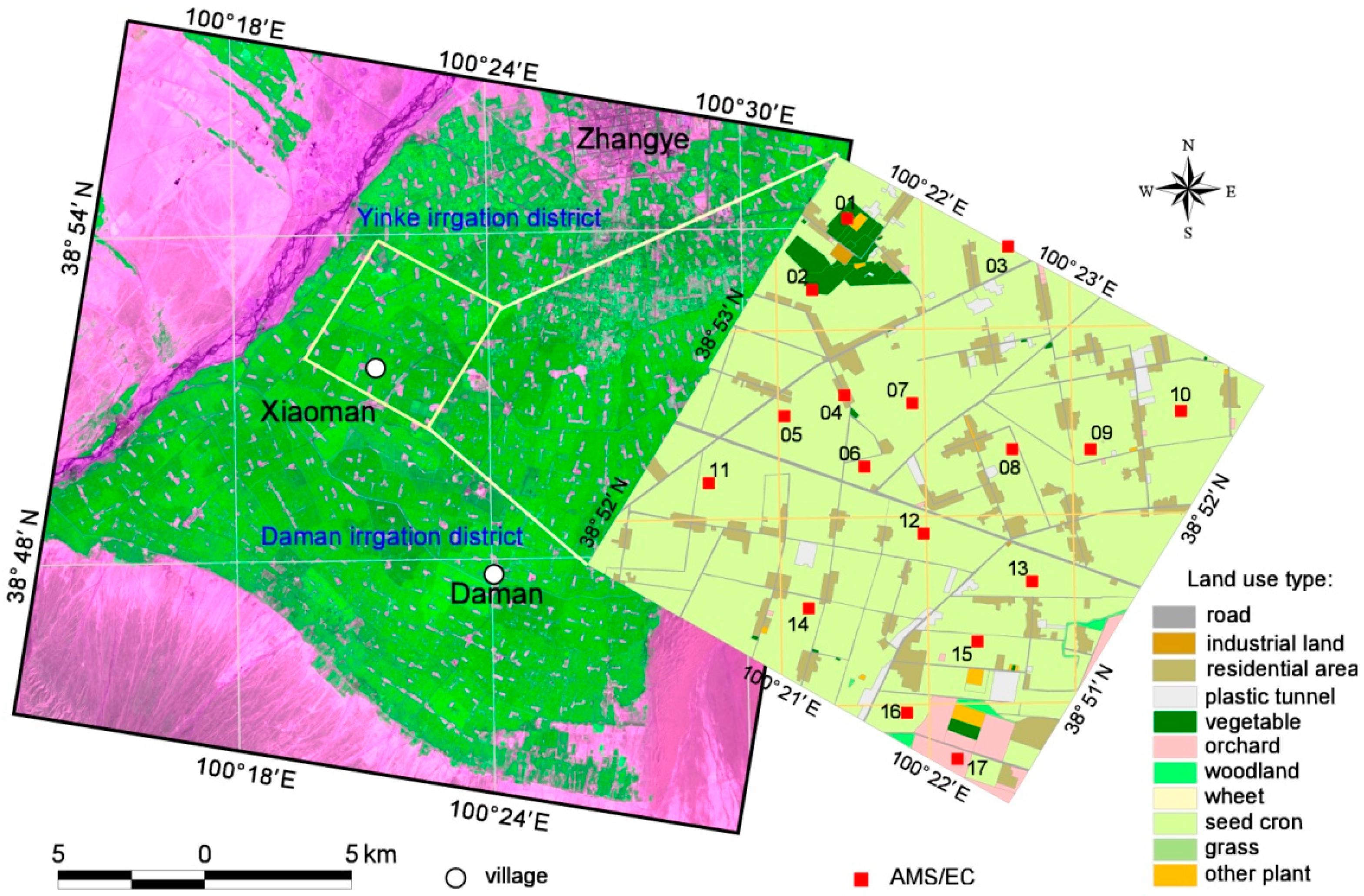
2.1. Field Observations

2.2. Satellite Images
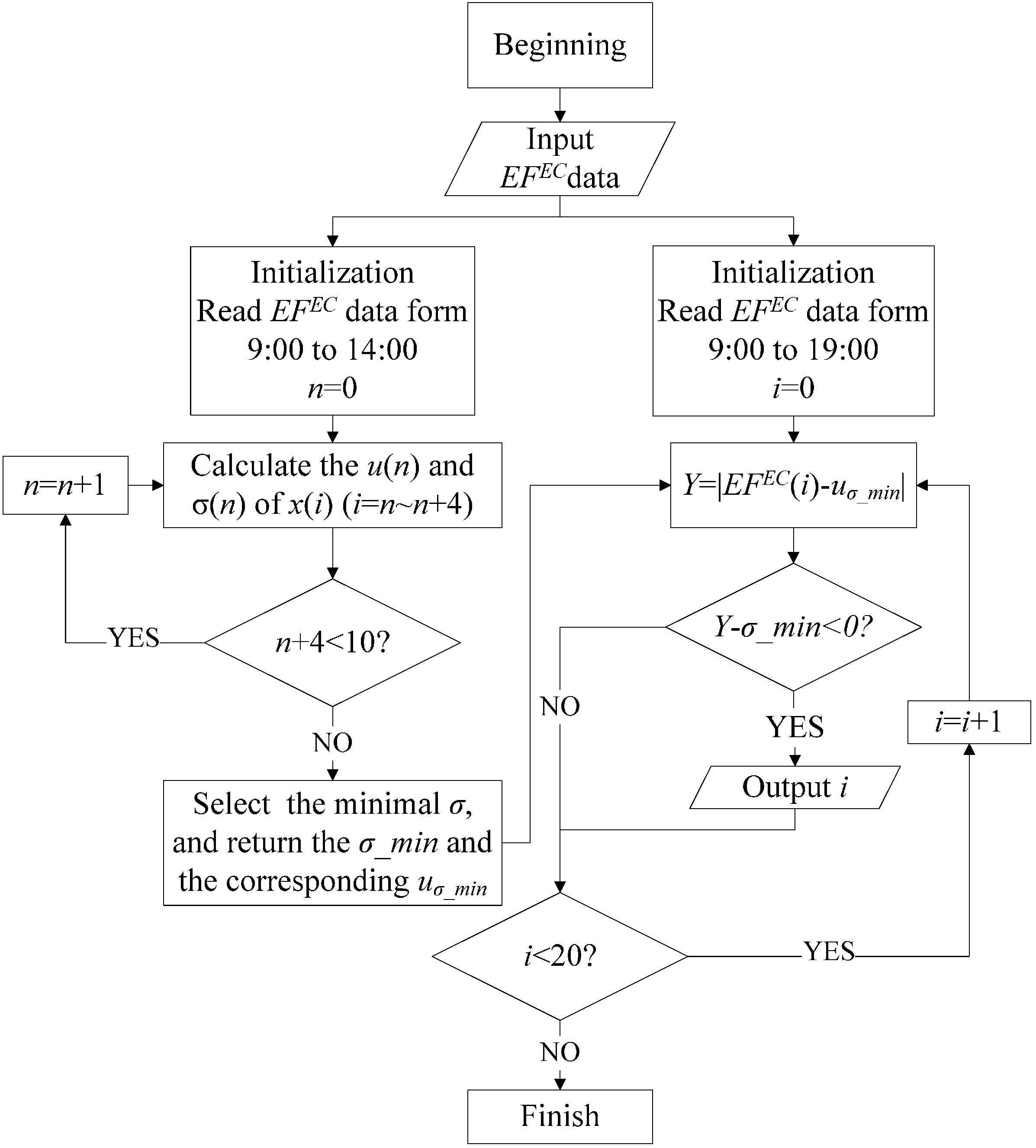
3. Methods
3.1. Constant EF Method (cEF)
3.2. Variable EF Method (vEF)
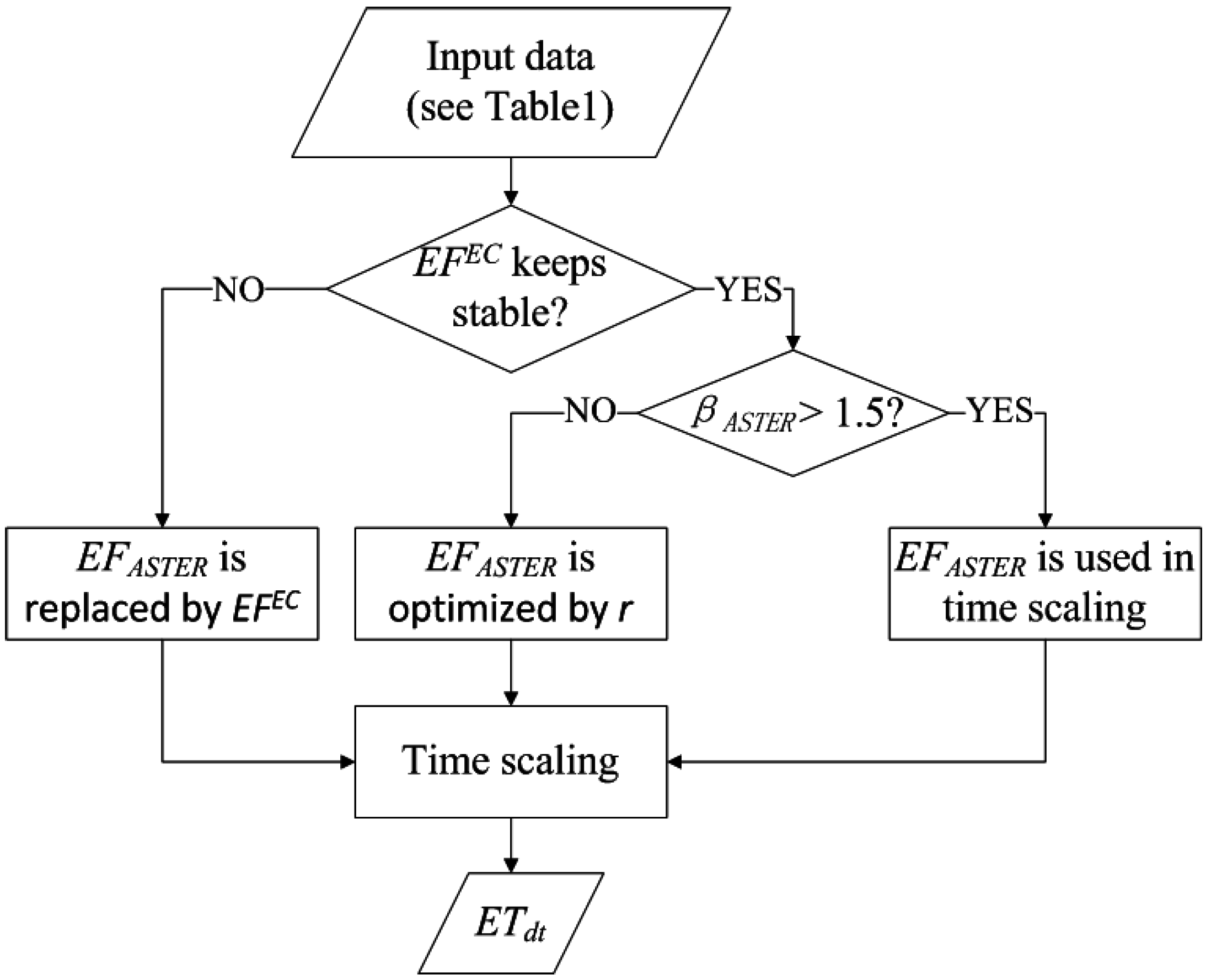
3.3. Revised Variable EF Method (vEFr)

| Methods | Spatial Input | Common Input |
|---|---|---|
| cEF | None | Midday constant EFASTER Half-hourly total solar radiation and half-hourly atmospheric long wave radiation Remotely sensed land surface emissivity Remotely sensed surface albedo Remotely sensed fc |
| vEF | Remotely sensed βASTER | |
| Adjustment factor calculated from meteorological observations | ||
| vEFr | Remotely sensed βASTER | |
| Adjustment factor calculated from meteorological observations | ||
| Half-hourly EFEC values |

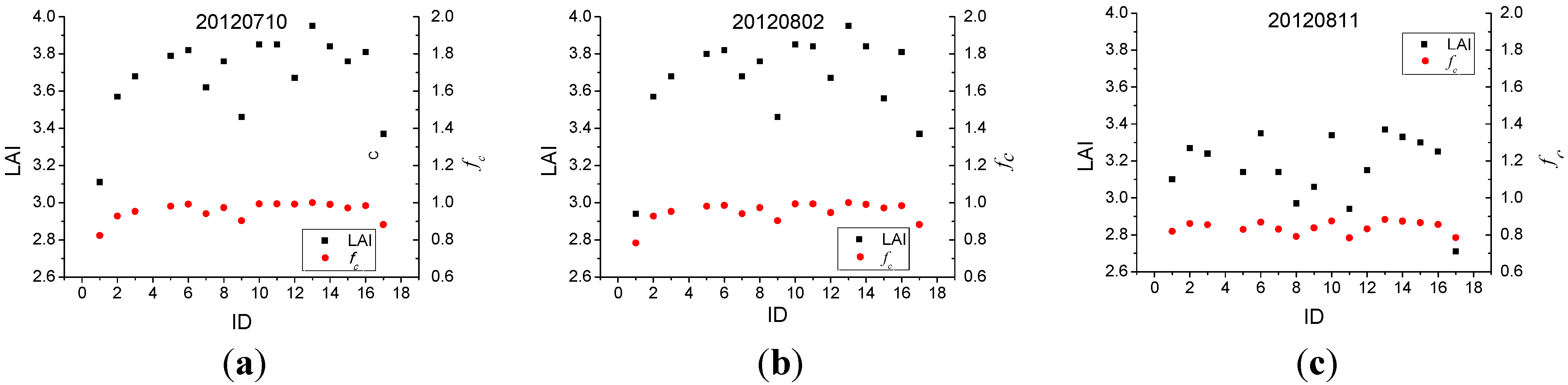
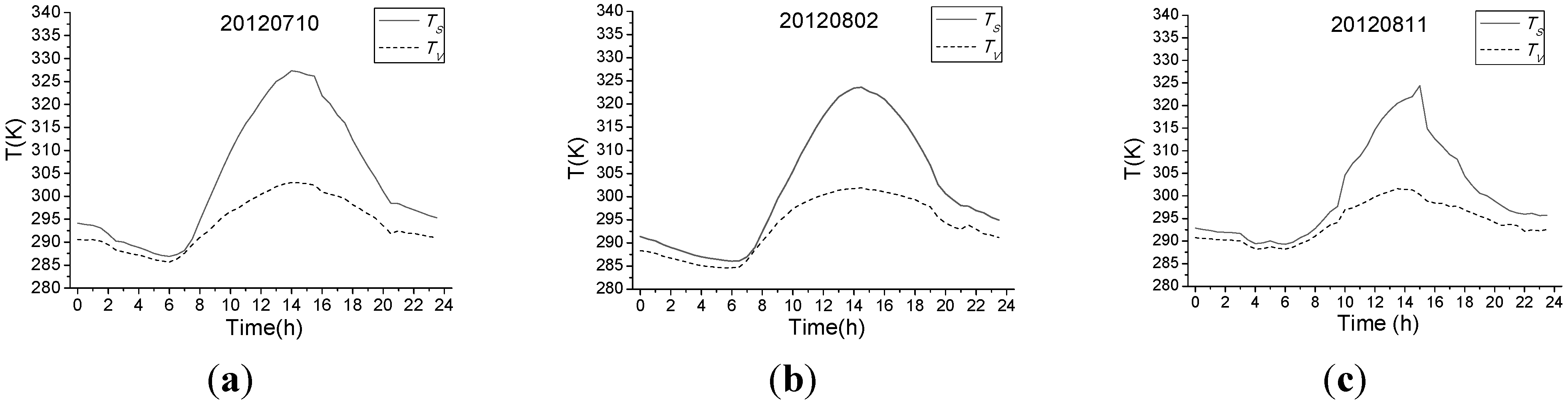
3.4. Remotely Sensed Estimation for Land Surface Variables
| Date (yyyy/mm/dd) | (K) | (K) | RMSE (K) | (K) | (K) | RMSE (K) |
|---|---|---|---|---|---|---|
| 20120710 | 300.48 | 26.67 | 1.87 | 296.88 | 4.81 | 1.12 |
| 20120802 | 300.62 | 23.90 | 1.37 | 293.60 | 8.94 | 1.45 |
| 20120811 | 300.91 | 15.44 | 3.64 | 294.14 | 6.50 | 1.52 |
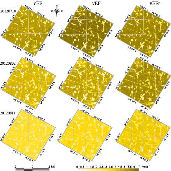
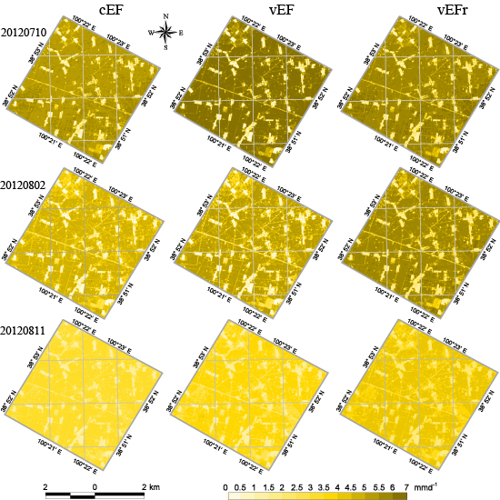
4. Results and Validation
| Date (yyyy/mm/dd) | Stable Time (In Hours on A 24-Hour Basis) |
|---|---|
| 20120710 | 11–16, 17.5 |
| 20120802 | 9–16, 17.5 |
| 20120811 | 9, 10–14.5 |


| EC ID | fc | EC | cEF | vEF | vEFr |
|---|---|---|---|---|---|
| EC01 | 0.8236 | 5.71 | 4.96 | 5.33 | 5.26 |
| EC02 | 0.9278 | 5.76 | 5.39 | 6.01 | 5.79 |
| EC03 | 0.9532 | 6.44 | 5.43 | 6.31 | 5.98 |
| EC04 | 0.0000 | 2.82 | 2.08 | 2.51 | 2.78 |
| EC05 | 0.9805 | 5.26 | 5.44 | 6.12 | 5.47 |
| EC06 | 0.9916 | 6.37 | 5.43 | 6.35 | 5.97 |
| EC07 | 0.9406 | 5.78 | 5.44 | 6.26 | 5.86 |
| EC08 | 0.9732 | 6.72 | 5.46 | 6.36 | 6.03 |
| EC09 | 0.9035 | 4.65 | 5.21 | 6.18 | 5.58 |
| EC10 | 0.9935 | 6.19 | 5.45 | 6.31 | 5.95 |
| EC11 | 0.9933 | 5.66 | 5.29 | 6.33 | 5.82 |
| EC12 | 0.9922 | 6.41 | 5.43 | 6.39 | 6.01 |
| EC13 | 1.0000 | 6.76 | 5.46 | 6.38 | 6.02 |
| EC14 | 0.9905 | 7.04 | 5.02 | 6.46 | 6.04 |
| EC15 | 0.9717 | 5.69 | 5.36 | 6.16 | 5.78 |
| EC16 | 0.9839 | 6.36 | 5.42 | 6.32 | 6.00 |
| EC17 | 0.8816 | 5.98 | 5.28 | 5.75 | 5.73 |
| EC ID | fc | EC | cEF | vEF | vEFr |
|---|---|---|---|---|---|
| EC01 | 0.7836 | 5.53 | 3.67 | 3.91 | 4.61 |
| EC02 | 0.9278 | 5.00 | 4.57 | 4.88 | 5.41 |
| EC03 | 0.9532 | 5.86 | 4.62 | 4.93 | 5.73 |
| EC04 | 0.0000 | 2.45 | 1.51 | 1.86 | 2.04 |
| EC05 | 0.9805 | 4.95 | 4.58 | 5.09 | 5.28 |
| EC06 | 0.9851 | 5.71 | 4.74 | 5.13 | 5.52 |
| EC07 | 0.9406 | 5.73 | 4.62 | 4.98 | 5.70 |
| EC08 | 0.9732 | 5.85 | 4.66 | 5.01 | 5.80 |
| EC09 | 0.9035 | 5.42 | 4.54 | 4.96 | 5.44 |
| EC10 | 0.9935 | 6.24 | 4.75 | 5.15 | 5.91 |
| EC11 | 0.9933 | 5.43 | 4.76 | 4.94 | 5.67 |
| EC12 | 0.9465 | 5.67 | 4.47 | 4.93 | 5.44 |
| EC13 | 1.0000 | 5.61 | 4.74 | 5.14 | 5.84 |
| EC14 | 0.9905 | 6.27 | 4.62 | 5.06 | 5.92 |
| EC15 | 0.9717 | 5.69 | 4.77 | 5.14 | 5.45 |
| EC16 | 0.9839 | 7.56 | 4.67 | 5.14 | 5.78 |
| EC17 | 0.8816 | 5.59 | 4.36 | 4.66 | 5.41 |
| EC ID | fc | EC | cEF | vEF | vEFr |
|---|---|---|---|---|---|
| EC01 | 0.8193 | 4.62 | 2.98 | 3.58 | 3.92 |
| EC02 | 0.8604 | 4.21 | 3.11 | 3.35 | 4.04 |
| EC03 | 0.8551 | 4.38 | 3.21 | 3.78 | 4.12 |
| EC04 | 0.0000 | 1.54 | 1.38 | 1.41 | 1.82 |
| EC05 | 0.8289 | 3.76 | 3.15 | 3.44 | 3.80 |
| EC06 | 0.8677 | 3.93 | 3.15 | 3.48 | 3.89 |
| EC07 | 0.8303 | 4.27 | 3.17 | 3.71 | 4.14 |
| EC08 | 0.7912 | 3.91 | 3.05 | 3.58 | 3.85 |
| EC09 | 0.8381 | 3.44 | 3.16 | 3.33 | 3.82 |
| EC10 | 0.8747 | 4.52 | 3.23 | 3.75 | 4.24 |
| EC11 | 0.7830 | 3.97 | 3.08 | 3.04 | 3.84 |
| EC12 | 0.8320 | 4.74 | 3.19 | 3.65 | 4.18 |
| EC13 | 0.8831 | 4.87 | 3.29 | 3.83 | 4.20 |
| EC14 | 0.8734 | 4.83 | 3.33 | 3.77 | 4.18 |
| EC15 | 0.8654 | 4.12 | 3.25 | 3.89 | 4.16 |
| EC16 | 0.8556 | 6.10 | 3.09 | 3.68 | 4.13 |
| EC17 | 0.7849 | 4.08 | 2.91 | 2.89 | 3.81 |
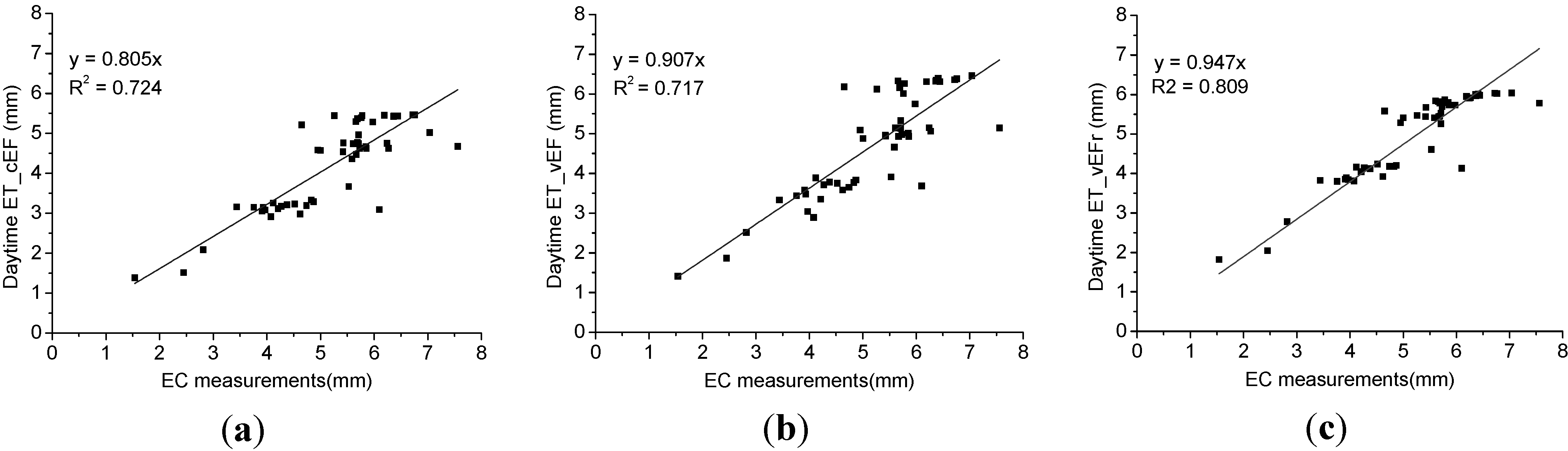
| cEF | vEF | vEFr | |
|---|---|---|---|
| RMSE (mm d−1) | 1.19 | 0.85 | 0.54 |
| MRE (%) | 19.97 | 12.77 | 7.26 |
| Corr. | 0.72 | 0.72 | 0.81 |
5. Discussion
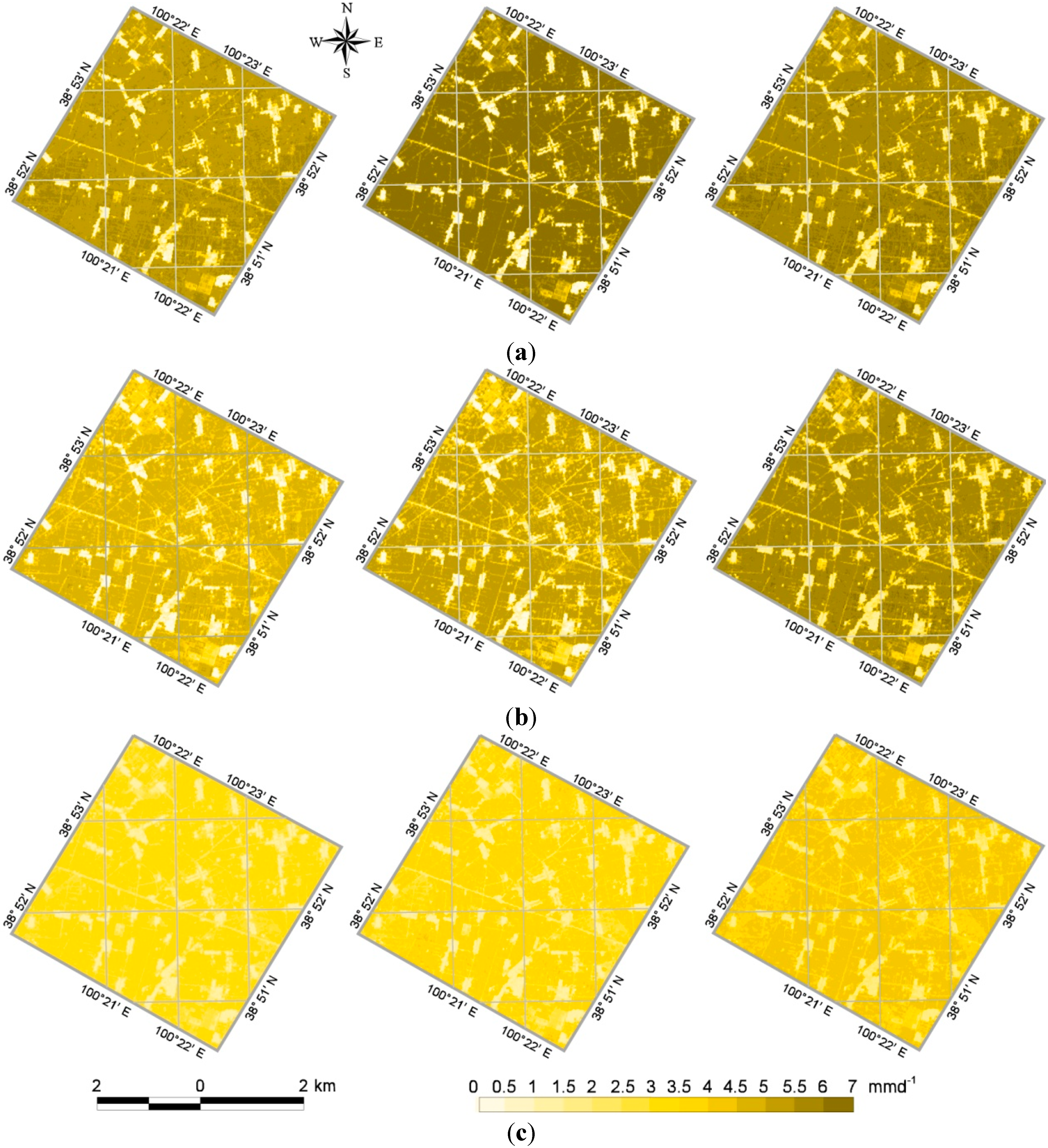
5.1. Spatial Heterogeneity of the EF
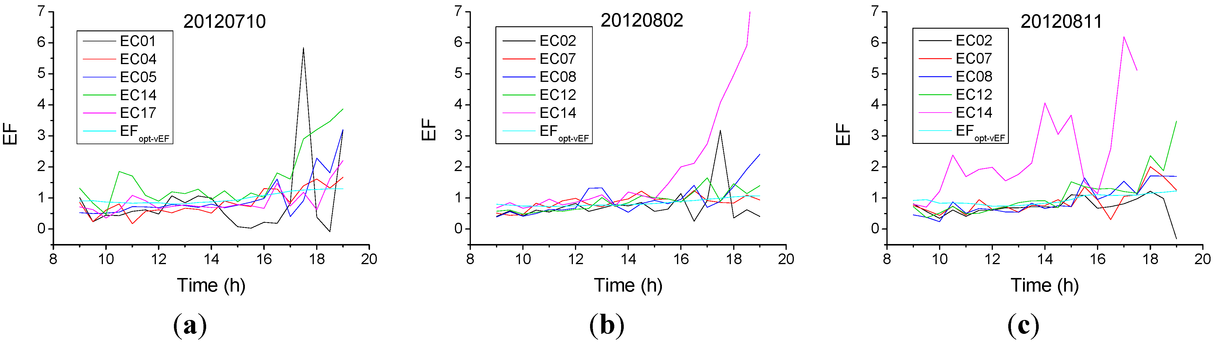
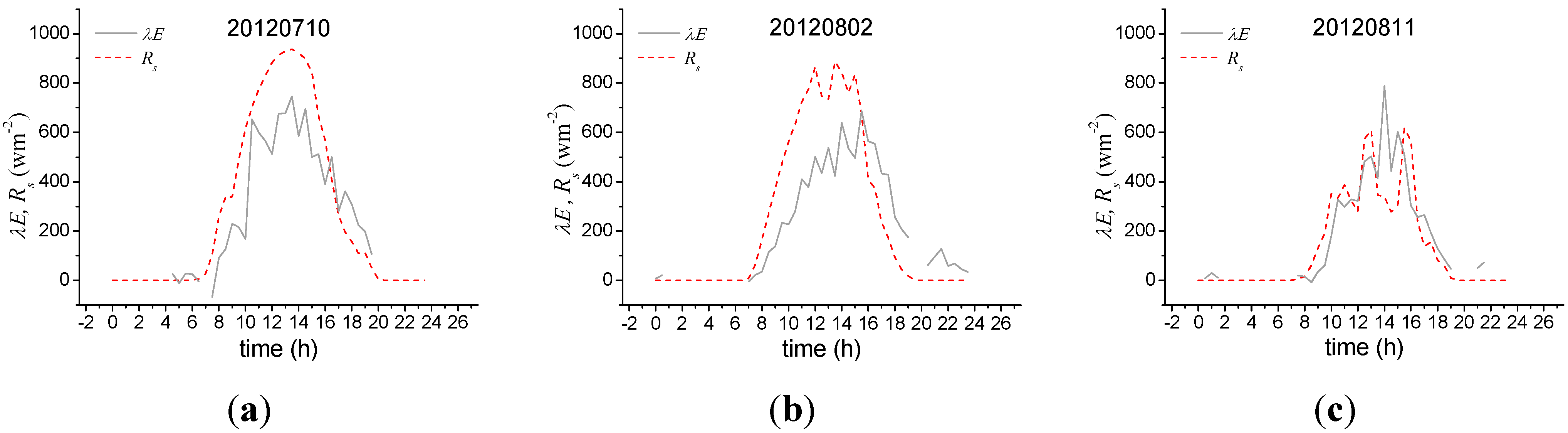
5.2. Temporal Heterogeneity of the EF

5.3. The Uncertainty in Input
5.4. The Saturation of fc

5.5. The Transferability and Limitations of vEFr
6. Conclusions
Acknowledgements
Author Contributions
Conflicts of Interest
References
- Bastiaanssen, W.G.M.; Molden, D.J.; Makin, I.W. Remote sensing for irrigated agriculture: Examples from research and possible applications. Agric. Water Manag. 2000, 46, 137–155. [Google Scholar] [CrossRef]
- Su, Z. Remote sensing of land use and vegetation for mesoscale hydrological studies. Int. J. Remote Sens. 2000, 21, 213–233. [Google Scholar] [CrossRef]
- Li, Z.; Tang, R.; Wan, Z.; Bi, Y.; Zhou, C.; Tang, B.; Yan, G.; Zhang, X. A review of current methodologies for regional evapotranspiration estimation from remotely sensed data. Sensors 2009, 9, 3801–3853. [Google Scholar] [CrossRef] [PubMed]
- Allen, R.G. Using the FAO-56 dual crop coefficient method over an irrigated region as part of an evapotranspiration intercomparison study. J. Hydrol. 2000, 229, 27–41. [Google Scholar] [CrossRef]
- Porporato, A.; Daly, E.; Rodriguez-Iturbe, I. Soil water balance and ecosystem response to climate change. Am. Nat. 2004, 164, 625–632. [Google Scholar] [CrossRef] [PubMed]
- Myneni, R.B.; Hoffman, S.; Knyazikhin, Y.; Privette, J.L.; Glassy, J.; Tian, Y.; Wang, Y.; Song, X.; Zhang, Y.; Smith, G.R.; et al. Global products of vegetation leaf area and fraction absorbed PAR from year one of MODIS data. Remote Sens. Environ. 2002, 83, 214–231. [Google Scholar] [CrossRef]
- Huete, A.; Didan, K.; Miura, T.; Rodriguez, E.P.; Gao, X.; Ferreira, L.G. Overview of the radiometric and biophysical performance of the MODIS vegetation indices. Remote Sens. Environ. 2002, 83, 195–213. [Google Scholar] [CrossRef]
- Chen, Y.; Xia, J.; Liang, S.; Feng, J.; Fisher, J.B.; Li, X.; Li, X.L.; Liu, S.; Ma, Z.; Miyata, A.; et al. Comparison of satellite-based evapotranspiration models over terrestrial ecosystems in China. Remote Sens. Environ. 2014, 140, 279–293. [Google Scholar] [CrossRef]
- Su, Z. The Surface Energy Balance System (SEBS) for estimation of turbulent heat fluxes. Hydrol. Earth Syst. Sci. 2002, 6, 85–99. [Google Scholar] [CrossRef]
- Bastiaanssen, W.G.M.; Menenti, M.; Feddes, R.A.; Holtslag, A.A. A remote sensing surface energy balance algorithm for land (SEBAL): I. Formulation. J. Hydrol. 1998, 212–213; 198–212. [Google Scholar] [CrossRef]
- Long, D.; Singh, V.P. A two-source trapezoid model for evapotranspiration (TTME) from satellite imagery. Remote Sens. Environ. 2012, 121, 370–388. [Google Scholar] [CrossRef]
- Xin, X.; Liu, Q. The Two-layer Surface Energy Balance Parameterization Scheme (TSEBPS) for estimation of land surface heat fluxes. Hydrol. Earth Syst. Sci. 2010, 14, 491–504. [Google Scholar] [CrossRef]
- Jackson, R.D.; Hatfield, J.L.; Reginato, R.J.; Idso, S.B.; Pinter, P.J. Estimation of daily evapotranspiration from one time of day measurements. Agric. Water Manag. 1983, 7, 351–362. [Google Scholar] [CrossRef]
- Sugita, M.; Brutsaert, W. Daily evaporation over a region from lower boundary layer profiles measured with radiosondes. Water Resour. Res. 1991, 27, 747–752. [Google Scholar] [CrossRef]
- Zhang, L.; Lemeur, R. Evaluation of daily evapotranspiration estimates from instantaneous measurements. Agric. For. Meteorol. 1995, 74, 139–154. [Google Scholar] [CrossRef]
- Allen, R.G.; Tasumi, M.; Trezza, R. Satellite-based energy balance for mapping evapotranspiration with internalized calibration (METRIC)-model. J. Irrig. Drain. Eng. 2007, 133, 380–394. [Google Scholar] [CrossRef]
- Tomás, A.; Nieto, H.; Guzinski, R.; Salas, J.; Sandholt, I.; Berliner, P. Validation and scale dependencies of the triangle method for the evaporative fraction estimation over heterogeneous areas. Remote Sens. Environ. 2014, 152, 493–511. [Google Scholar] [CrossRef]
- Crago, R.D. Conservation and variability of the evaporative fraction during the daytime. J. Hydrol. 1996, 180, 173–194. [Google Scholar] [CrossRef]
- Hoedjes, J.C.B.; Chehbouni, A.; Jacob, F.; Ezzahar, J.; Boulet, G. Deriving daily evapotranspiration from remotely sensed instantaneous evaporative fraction over olive orchard in semi-arid Morocco. J. Hydrol. 2008, 354, 53–64. [Google Scholar] [CrossRef]
- Gentine, P.; Entekhabi, D.; Chehbouni, A.; Boulet, G.; Duchemin, B. Analysis of evaporative fraction diurnal behavior. Agric. For. Meteorol. 2007, 143, 13–29. [Google Scholar] [CrossRef] [Green Version]
- Gentine, P.; Entekhabi, D.; Polcher, J. The diurnal behavior of evaporative fraction in the soil-vegetation-atmospheric boundary layer continuum. J. Hydrometeorol. 2011, 12, 1530–1546. [Google Scholar] [CrossRef]
- Lu, J.; Tang, R.; Tang, H.; Li, Z. Derivation of daily evaporative fraction based on temporal variations in surface temperature, air temperature, and net radiation. Remote Sens. 2013, 5, 5369–5396. [Google Scholar] [CrossRef]
- Suleiman, A.; Crago, R.D. Hourly and daytime evapotranspiration from grassland using radiometric surface temperatures. Agron. J. 2004, 96, 384–390. [Google Scholar] [CrossRef]
- Cheng, G.; Li, X.; Zhao, W.; Xu, Z.; Feng, Q.; Xiao, S.; Xiao, H. Integrated study of the water-ecosystem-economy in the Heihe River Basin. Natl. Sci. Rev. 2014, 1, 413–428. [Google Scholar] [CrossRef]
- Yang, D.; Chen, H.; Lei, M. Analysis of the diurnal pattern of evaporative fraction and its controlling factors over croplands in the Northern China. J. Integr. Agric. 2013, 12, 1316–1329. [Google Scholar] [CrossRef]
- Li, X.; Cheng, G.; Liu, S.; Xiao, Q.; Ma, M.; Jin, R.; Che, T.; Liu, Q.; Wang, W.; Qi, Y.; et al. Heihe Watershed Allied Telemetry Experimental Research (HiWATER): Scientific objectives and experimental design. Bull. Am. Meteorol. Soc. 2013, 94, 1145–1160. [Google Scholar] [CrossRef]
- Xu, Z.; Liu, S.; Li, X.; Shi, S.; Wang, J.; Zhu, Z.; Xu, T.; Wang, W.; Ma, M. Intercomparison of surface energy flux measurement systems used during the HiWATER-MUSOEXE. J. Geophys. Res. 2013, 118, 13140–13157. [Google Scholar]
- Vickers, D.; Mahrt, L. Quality control and flux sampling problems for tower and aircraft data. J. Atmos. Ocean. Technol. 1997, 14, 512–526. [Google Scholar] [CrossRef]
- Wilczak, J.M.; Oncley, S.P.; Stage, S.A. Sonic anemometer tilt correction algorithms. Bound.-Layer Meteorol. 2001, 99, 127–150. [Google Scholar] [CrossRef]
- Schotanus, P.; Nieuwstadt, F.T.M.; DeBruin, H.A.R. Temperature measurementwith a sonic anemometer and its application to heat and moisture fluctuations. Bound.-Layer Meteorol. 1983, 26, 81–93. [Google Scholar] [CrossRef]
- Moore, C.J. Frequency response corrections for eddy correlation systems. Bound.-Layer Meteorol. 1986, 37, 17–35. [Google Scholar] [CrossRef]
- Webb, E.K.; Pearman, G.I.; Leuning, R. Correction of the flux measurements for density effects due to heat and water vapour transfer. Q. J. R. Meteorol. Soc. 1980, 106, 85–100. [Google Scholar] [CrossRef]
- Liu, S.; Xu, Z.; Wang, W.; Bai, J.; Jia, Z.; Zhu, M.; Wang, J. A comparison of eddy-covariance and large aperture scintillometer measurements with respect to the energy balance closure problem. Hydrol. Earth Syst. Sci. 2011, 15, 1291–1306. [Google Scholar] [CrossRef]
- Colaizzi, P.D.; Evett, S.R.; Howell, T.A.; Tolk, J.A. Comparison of five models to scale daily evapotranspiration from one-time-of-day measurements. Trans. ASAE 2006, 49, 1409–1417. [Google Scholar] [CrossRef]
- Song, Y.; Wang, J.; Yang, K.; Ma, M.; Li, X.; Zhang, Z.; Wang, X. A revised surface resistance parameterisation for estimating latent heat flux from remotely sensed data. Int. J. Appl. Earth Obs. Geoinf. 2012, 17, 76–84. [Google Scholar] [CrossRef]
- Yang, K.; Wang, J. A temperature prediction–correction method for estimating surface soil heat flux from soil temperature and moisture data. Sci. China Series D: Earth Sci. 2008, 51, 721–729. [Google Scholar] [CrossRef]
- Jia, Z.; Liu, S.; Xu, Z.; Chen, Y.; Zhu, M. Validation of remotely sensed evapotranspiration over the Hai River Basin, China. J. Geophys. Res. 2012, 117. [Google Scholar] [CrossRef]
- Kormann, R.; Meixner, F. An analytical footprint model for non-neutral stratification. Bound.-Layer Meteorol. 2001, 99, 207–224. [Google Scholar] [CrossRef]
- Jacob, F.; Olioso, A. Derivation of diurnal courses of albedo and reflected solar irradiance from airborne POLDER data acquired near solar noon. J. Geophys. Res. 2005, 110. [Google Scholar] [CrossRef]
- Liang, S. Narrowband to broadband conversions of land surface albedo: I Algorithms. Remote Sens. Environ. 2001, 76, 213–238. [Google Scholar] [CrossRef]
- Sobrino, J.A.; Jimenez-Munoz, J.C.; Soria, G.; Romaguera, M.; Guanter, L.; Moreno, J.; Plaza, A.; Martinez, P. Land surface emissivity retrieval from different VNIR and TIR sensors. IEEE Trans. Geosci. Remote Sens. 2008, 46, 316–327. [Google Scholar] [CrossRef]
- Qin, Z.; Karnieli, A. A mono-window algorithm for retrieving land surface temperature from Landsat TM data and its application to the Israel-Egypt border region. Int. J. Remote Sens. 2001, 22, 3719–3746. [Google Scholar] [CrossRef]
- Carlson, T.N.; Ripley, D.A. On the relation between NDVI, fractional vegetation cover and leaf area index. Remote Sens. Environ. 1997, 62, 241–252. [Google Scholar] [CrossRef]
- Wan, Z.; Zhang, Y.; Zhang, Q.; Li, Z. Validation of the landsurface temperature products retrieved from Terra Moderate Resolution Imaging Spectroradiometer data. Remote Sens. Environ. 2002, 83, 163–180. [Google Scholar] [CrossRef]
- Monteith, J.L. Principles of Environmental Physics; Edward Arnold: London, UK, 1973; p. 241. [Google Scholar]
- Kustas, W.P.; Daughtry, C.S.T. Estimation of the soil heat flux/net radiation ratio from spectral data. Agric. For. Meteorol. 1989, 49, 205–223. [Google Scholar] [CrossRef]
- Wu, B.; Yan, N.; Xiong, J.; Bastiaanssen, W.G.M.; Zhu, W.; Stein, A. Validation of ETWatch using field measurements at diverse landscapes: A case study in Hai Basin of China. J. Hydrometeorol. 2012, 436–437, 67–80. [Google Scholar]
- Wang, J.; Zhuang, J.; Wang, W.; Liu, S.; Xu, Z. Assessment of uncertainties in eddy covariance flux measurement based on intensive flux matrix of HiWATER-MUSOEXE. IEEE Geosci. Remote Sens. Lett. 2014, 12, 259–263. [Google Scholar] [CrossRef]
- Kohsiek, W.; Liebethal, C.; Foken, T.; Vogt, R.; Oncley, S.P.; Bernhofer, C.; Debruin, H.A.R. The energy balance experiment EBEX-2000. Part III: Behaviour and quality of the radiation measurements. Bound.-Layer Meteorol. 2007, 123, 55–75. [Google Scholar] [CrossRef]
- Wen, X.; Lee, X.; Sun, X.; Wang, J.; Hu, Z.; Li, S.; Yu, G. Dew water isotopicratios and their relations to ecosystem water pools and fluxes in a cropland and a grassland in China. Oecologia. 2012, 168, 549–561. [Google Scholar] [CrossRef] [PubMed]
- Swinbank, W.C. Measurement of vertical transfer of heat and water vapour by eddies in the low atmosphere. J. Meteorol. 1951, 8, 135–145. [Google Scholar] [CrossRef]
- Thornthwait, C.W.; Holzman, A. Report of the commutation on transpiration and evaporation. Trans. Am. Geophys. Union 1944, 25, 683–693. [Google Scholar] [CrossRef]
© 2015 by the authors; licensee MDPI, Basel, Switzerland. This article is an open access article distributed under the terms and conditions of the Creative Commons Attribution license (http://creativecommons.org/licenses/by/4.0/).
Share and Cite
Song, Y.; Ma, M.; Jin, L.; Wang, X. A Revised Temporal Scaling Method to Yield Better ET Estimates at a Regional Scale. Remote Sens. 2015, 7, 6433-6453. https://doi.org/10.3390/rs70506433
Song Y, Ma M, Jin L, Wang X. A Revised Temporal Scaling Method to Yield Better ET Estimates at a Regional Scale. Remote Sensing. 2015; 7(5):6433-6453. https://doi.org/10.3390/rs70506433
Chicago/Turabian StyleSong, Yi, Mingguo Ma, Long Jin, and Xufeng Wang. 2015. "A Revised Temporal Scaling Method to Yield Better ET Estimates at a Regional Scale" Remote Sensing 7, no. 5: 6433-6453. https://doi.org/10.3390/rs70506433