Image Segmentation Based on Constrained Spectral Variance Difference and Edge Penalty

Abstract

Segmentation, which is usually the first step in object-based image analysis (OBIA), greatly influences the quality of final OBIA results. In many existing multi-scale segmentation algorithms, a common problem is that under-segmentation and over-segmentation always coexist at any scale. To address this issue, we propose a new method that integrates the newly developed constrained spectral variance difference (CSVD) and the edge penalty (EP). First, initial segments are produced by a fast scan. Second, the generated segments are merged via a global mutual best-fitting strategy using the CSVD and EP as merging criteria. Finally, very small objects are merged with their nearest neighbors to eliminate the remaining noise. A series of experiments based on three sets of remote sensing images, each with different spatial resolutions, were conducted to evaluate the effectiveness of the proposed method. Both visual and quantitative assessments were performed, and the results show that large objects were better preserved as integral entities while small objects were also still effectively delineated. The results were also found to be superior to those from eCongnition’s multi-scale segmentation.

1. Introduction

The launch of a number of commercial satellites such as IKONOS, GeoEye and WorldView-1, 2, and 3 in the late 1990s has been an exciting development in the field of remote sensing. These satellites provide improved capability to acquire high spatial resolution images. Compared with low and medium resolution images, high spatial resolution images are endowed with more detailed spatial information; however, this detail poses great challenges for traditional image processing approaches, such as pixel-based image classification. Although successfully applied to low and moderate spatial resolution data, pixel-based classification schemes, which treat single pixels as processing units without considering contextual relationships with neighboring pixels, are not sufficient for high spatial resolution data. Because of the well-known issues of spectral and spatial heterogeneity, pixel-based classification often results in a large amount of misclassified noise. As an alternative, object-based image analysis (OBIA or GEOBIA) approaches were developed to classify high spatial resolution data [1,2,3,4,5]. OBIA first partitions imagery into segments, which are homogeneous groups of pixels (often referred to as objects). Then the image classification is performed on the objects (rather than pixels) using various types of information extracted from the objects, such as mean spectral values, shapes, textures and other object-level summary statistics. Since it is the image segmentation process that generates image objects and determines the attributes of the objects, the quality of the segmentation significantly influences the final results of OBIA.

Image segmentation has long been studied in the field of computer vision, and has been widely applied in industrial and medical image processing [6,7]. In the field of remote sensing, image segmentation gained popularity in the late 1990s [8], and numerous segmentation algorithms have since been developed. Generally, segmentation algorithms applied in remote sensing can be classified as point-based, edge-based, region-based or hybrids [9,10,11].

Point-based algorithms usually apply global information of entire image to search and label homogeneous pixels without considering neighborhood [10]. The most well-known point-based algorithm is histogram thresholding segmentation, which assumes, that valleys exist in histogram between different classes. Generally, histogram thresholding includes three steps: histogram modes recognizing, valleys (thresholds) between modes searching and thresholds applying [12]. Point-based methods are simple and quick, but require that different classes have evidently different values in the images. This method may encounter difficulty when processing remotely sensed imagery of a large coverage that exhibits inter-class spectral similarity and intra-class heterogeneity, which may severely deform the histogram modes. Therefore, the histogram thresholding segmentation method is usually applied in the delineation of local objects [12].

Edge-based algorithms exploit the possible existence of a perceivable edge between objects. The two best known algorithms are optimal edge detector [12,13] and watershed segmentation [14,15]. The optimal edge detector first uses the Canny operator [16] to detect edges and then the “best count” method is utilized to close the edge contours [17]. Watershed segmentation first extracts the gradient information from the original image, and the watershed transformation is then applied to the gradients to generate basins and watersheds. The basins represent the segments and the watersheds the division between them. Edge-based algorithms can quickly partition images; the process is highly accurate for images with obvious edges. However, because edge-based algorithms are primarily based on local contrasts, they are particularly sensitive to noise, which may lead to over-segmentation where a real world object is incorrectly partitioned into several small objects. Additionally, because most edge-based algorithms rely on the step edge model [12,18,19], they are less sensitive to “blurry” boundaries, which may lead to under-segmentation where all or part of a real world object is incorrectly combined with another object.

Because of these defects with edge-based segmentation algorithms, region-based approaches were developed and are widely used. Region-based approaches use regions as the basic unit. Attributes of regions are extracted to represent heterogeneity or homogeneity. Heterogeneous regions are then separated and homogeneous regions are merged to form segments. Two major region-based algorithms are the split-and-merge algorithm [20] and the region-growing algorithm [21,22]. The split-and-merge algorithm begins by treating the entire image as a single region. Regions are then iteratively split into sub-regions (usually 4 regions via a quad tree) according to a homogeneity/heterogeneity criterion. The splitting continues until all the regions become homogeneous. A final stage merges homogeneous regions and ensures that neighboring objects are heterogeneous. The region-growing algorithm begins from a set of seed pixels that are successively merged with neighboring pixels according to a heterogeneity/homogeneity criterion. The merging ends when all the pixels are merged and all neighboring objects are heterogeneous. The most significant problem of region-based algorithm is that segmentation errors often occur along the boundaries between regions.

To combine the advantages of edge-based and region-based methods, increasingly more researchers have developed hybrid approaches. For example, Pavlidis and Liow [23] and Cortez et al. [24] used the edges generated by edge detection to refine the boundary of split-and-merging segmentation to improve the results. Haris et al. [25] and Castilla, Hay and Ruiz [26] used watersheds for initial segmentation and then merged these initial segments via a region-merging algorithm. Yu and Clausi [27] and Zhang et al. [28,29] added edge information as part of the merging criterion (MC) of a region growing algorithm. These hybrid methods generally provide superior results when compared with those of edge-based or region-based methods.

Among existing algorithms, multi-scale segmentation, used by the eCognition software, has been the most widely employed. For example, Baatz and Schäpe [22] adopted a region-growing method using spectral and form heterogeneity changes as merging criteria to generate multi-resolution results. Robinson, Redding and Crisp [30] employed a similar approach by combining spectral variance difference (SVD) and common boundary length as the MC. Zhang et al. [28,29] employed a hybrid method that integrated edge penalty (EP) and standard deviation changes as merging criteria to generate multi-scale segmentation. In these multi-scale segmentation algorithms, the concept of scale plays a key role. However, scale as a threshold for MC often leads to similarly sized segments [22], but the real world is more complicated and contains objects with a large variation in size. Partitioning the image into segments similar in size may simultaneously cause over-segmentation and under-segmentation at a specific scale [31]. The solution to this problem, as offered by the multi-scale approach, is to segment images into differently scaled segmented layers that are linked by an object relation tree; this technique is known as the Fractal Net Evaluation Approach (FNEA) [32]. In FNEA, a layer of segments generated by a specific scale parameter is called an image-object level. Objects at a higher image-object level, in which the scale parameter is larger, are merged from the objects derived from a lower level. Consequently, the same real world objects may have a number of representations at different scale levels. To utilize the information at different scales, multi-scale classification must analyze the attributes of various objects at different scales and construct corresponding classification rules. As a result, the analysis in multi-scale segmentation can become formidably complicated.

The goal of this study is to develop a new segmentation algorithm that can generate various-sized image objects that are close to their real world counterparts using a single scale parameter. Many existing algorithms [22,30,32,33,34,35,36,37] use SVD as a MC to describe changes in spectral heterogeneity. However, the SVD is excessively influenced by the object sizes, which is the main cause for the simultaneous over-segmentation and under-segmentation. To address this problem, the proposed approach devises a constrained SVD (CSVD) in the MC to limit the influence of the segment size. Additionally, an EP is incorporated into the MC to increase boundary accuracy. Given these characteristics, the proposed algorithm can be categorized as a hybrid segmentation method.

Similar to some other region-based approaches, the proposed approach adopted a three-step strategy. Firstly, a fast scan [37] was applied to produce an over-segmented result. In this stage, every pixel was first treated as a segment, and then the SVD was used as a simple MC to quickly partition the image. In the second stage, a more complex MC based on CSVD and EP was employed to continue the merging process. Region adjacent graph (RAG) [38,39] and nearest neighbor graph (NNG) [25] were used to expedite the merging process. Moreover, the global mutual best-fitting [22] strategy was employed to optimize the merging process. In the third and final stage, minor objects with size smaller than a pre-defined threshold were merged into their most similar neighboring objects to eliminate remaining noise.

In order to assess the performance of the proposed method, we performed two groups of experiments. In the first experiment, different parameters of the proposed algorithm were tested to analyze their effects on segmentation performance. For the key parameters, both visual and quantitative assessments were provided. In the second experiment, the results of the proposed method were compared to those from eCognition based on both visual and quantitative assessments. In those quantitative assessments, the rate of over-, under- and well-segmentation was used to evaluate the segmentation quality on small, medium and large objects. Results showed that the proposed algorithm was able to segment the objects properly well regardless of their size using single scale parameter, meanwhile, achieved higher accuracy compared to eCognition multi-scale segmentation.

Section 2 presents the study area and data, followed by Section 3 where the proposed method is described in detail. Section 4 shows the experimental results. Finally, conclusions and discussions are provided in Section 5.

2. Study Area and Data

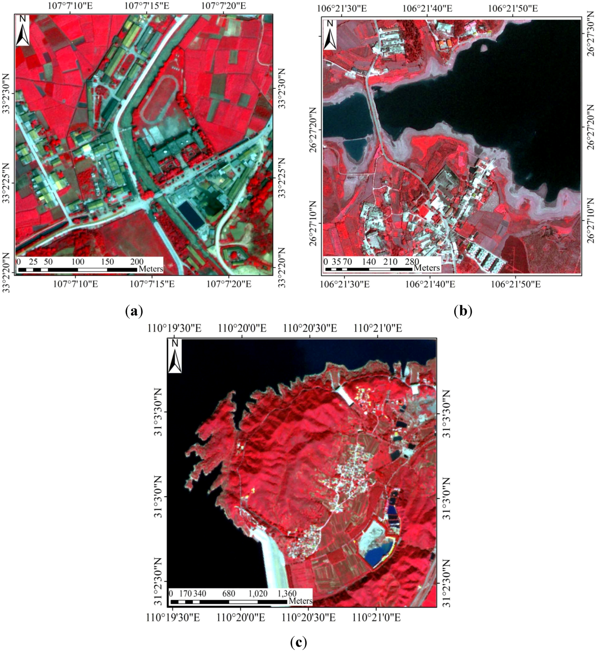
Three sets of images with different spatial resolutions, WorldView 2, an aerial image and RapidEye (Figure 1), were chosen as test datasets. Table 1 gives the basic information for these images. Figure 1a shows a pan-sharpened WorldView-2 image with a resolution of 0.6 m; the image covers an area in Hanzhong, China, where the main land cover types are farmland, road and buildings. Figure 1b is an aerial image with a resolution of 1 m covering part of the Three Gorges area, China, containing a small village, farmland and part of a river. Figure 1c is a subset of a RapidEye image for Miyun, China with a spatial resolution of 5 m. A residential area and farmland are located in the center of the image. The upper-left area (colored black in Figure 1c) is a reservoir, and the remainder is mainly forest. For convenience, Figure 1a–c are hereafter referred to as R1, R2 and R3, respectively. All have 4 bands (blue, green, red and NIR), stretched to the 0–255 gray scale for parameter comparability.

Figure 1. Images of test data. (a) A WorldView-2 image; (b) An aerial image; (c) A RapidEye image. The specific parameters of these images are listed in Table 1.

Figure 1. Images of test data. (a) A WorldView-2 image; (b) An aerial image; (c) A RapidEye image. The specific parameters of these images are listed in Table 1.

Table 1. Specific parameters of the test images.

Image	Platform	Size	Spatial Resolution	Position	Code
a	WorldView-2	872 × 896	0.6 m	Hanzhong	R1
b	Aerial plane	835 × 835	1 m	Three Gorges	R2
c	RapidEye	622 × 597	5 m	Miyun	R3

Table 1. Specific parameters of the test images.

Image	Platform	Size	Spatial Resolution	Position	Code
a	WorldView-2	872 × 896	0.6 m	Hanzhong	R1
b	Aerial plane	835 × 835	1 m	Three Gorges	R2
c	RapidEye	622 × 597	5 m	Miyun	R3

3. Methodology

The proposed method comprises the following general steps (Figure 2). Initial segments are first produced by a fast scan method. The RAG and NNG are then built based on the initial segmentation. Region merging is applied to the RAG and NNG by using CSVD and EP. Finally, minor objects are eliminated to generate the final result. The segmentation results are quantitatively assessed by an empirical discrepancy method.

Figure 2. General steps of the proposed method.

Figure 2. General steps of the proposed method.

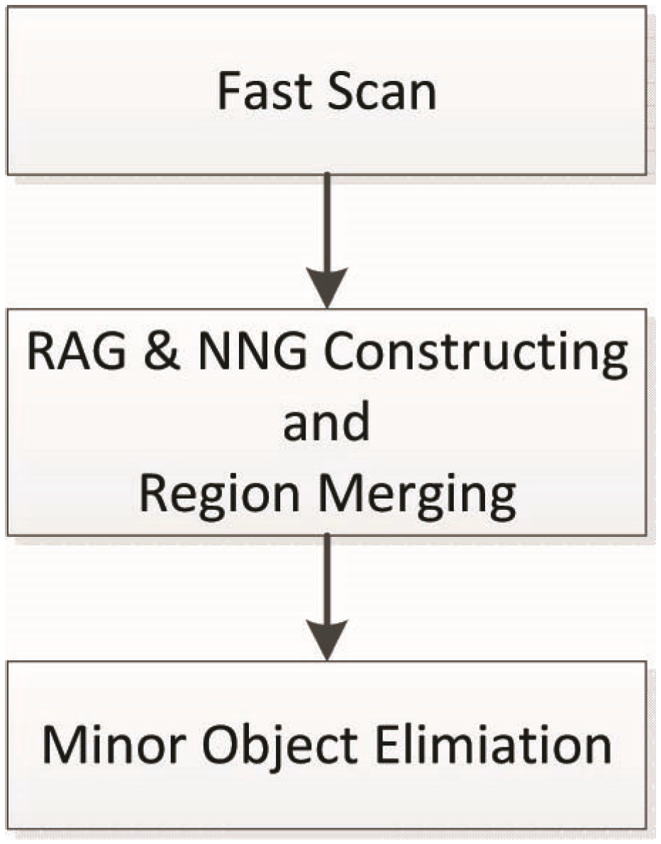
3.1. Initial Segmentation

The objective of initial segmentation is to quickly generate segments for the subsequent region-merging step. In this stage, over-segmentation is allowed, but under-segmentation should be avoided.

The initial segmentation is conducted by a quick scan of every pixel from the top-left to the bottom-right of the image. During the scan, each pixel is considered an image object and is compared to its upper-left neighboring objects. If the calculated MC is smaller than a given threshold, then the pixel object is merged with its neighboring object. In this step, only the spectral heterogeneity difference is used as the MC, formulated as follows [22]:

$$h_{diff}=(n_1+n_2)h_m-(n_1{h}_1+n_2{h}_2)$$

(1)

where h₁, h₂ are the heterogeneity of two adjacent objects before merging, h_m is the heterogeneity after h₁ and h₂ are merged, and n represents the object size.

The heterogeneity h can be computed as the variance of the object:

$$h=\frac{{\displaystyle \sum _{i=1}^n{(x_i-\mu )}^2}}{n}=\frac{{\displaystyle \sum _{i=1}^n{x_i}^2-n{\mu }^2}}{n}=\frac{SS-n{\mu }^2}{n}$$

(2)

where x is the spectral value of each pixel in an object, μ is the mean spectral value of the object, and SS represents the sum of squares of the pixel values.

Applying Equation (2) to Equation (1), we obtain the following:

$$h_{diff}=S{S}_m-(n_1+n_2){{\mu }_m}^2-(S{S}_1-n_1{{\mu }_1}^2)-(S{S}_2-n_2{{\mu }_2}^2)$$

(3)

where SS₁, SS₂ is sum of squares before merging, SS_m is sum of squares after merging.

Two hidden relationships exist:

$$(n_1+n_2){\mu }_m=n_1{\mu }_1+n_2{\mu }_2$$

(4)

$$S{S}_m=S{S}_1+S{S}_2$$

(5)

By applying Equations (4) and (5) to Equation (3), we obtain the final spectral heterogeneity difference, which is also referred to as SVD:

$$h_{diff}=SVD=\frac{n_1{n}_2}{n_1+n_2}{({\mu }_1-{\mu }_2)}^2=f(n_1,n_2)\cdot {({\mu }_1-{\mu }_2)}^2$$

(6)

where f(n₁,n₂) denotes $\frac{n_1{n}_2}{n_1+n_2}$.

For an image with b bands, the final SVD is the following:

$$SVD=\frac{{\displaystyle \sum _{i=1}^{b}SV{D}_i}}{b}=f(n_1,n_2)\cdot \frac{{\displaystyle \sum _{i=1}^b{({\mu }_1-{\mu }_2)}^2}}{b}$$

(7)

3.2. RAG and NNG Constructing and Region Merging

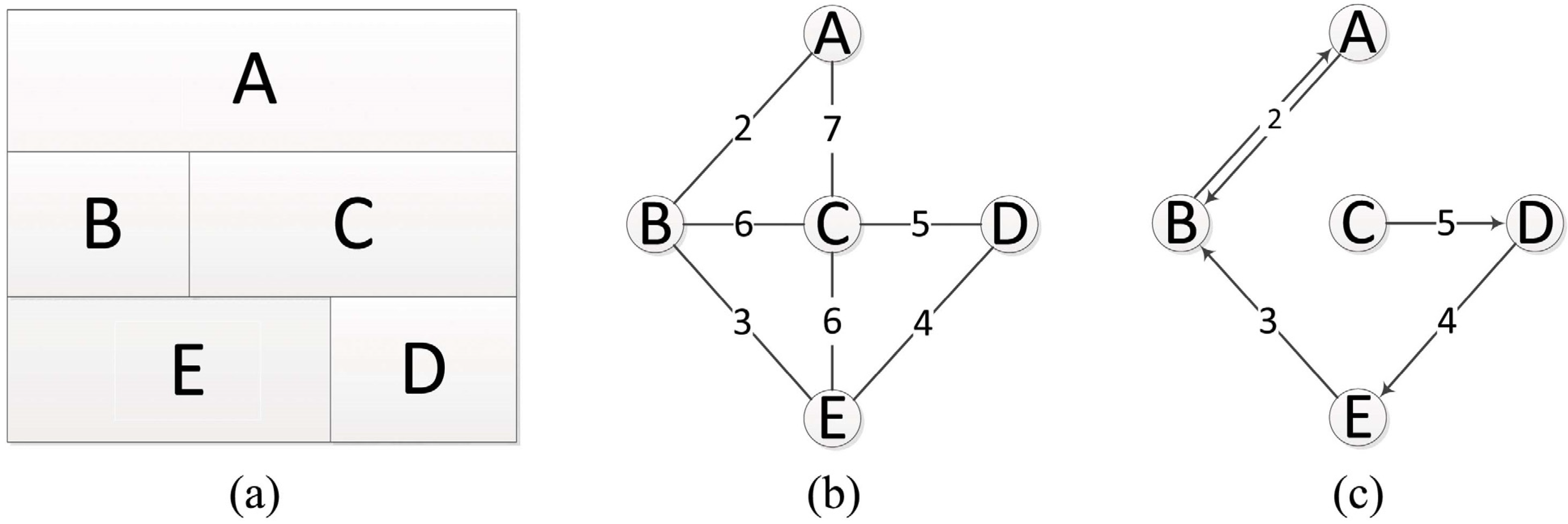
3.2.1. RAG and NNG Construction

RAG is a data structure which describes the segments and their relationships, defined as:

G = (V, E)

(8)

where V is the set of segments, called nodes, and E is the set of edges each of which stands for a neighborhood of two adjacent nodes. Each node carries particular object-level information, including the object ID, size, mean spectral value, and location. Each edge contains information, such as the IDs of adjacent objects, their dissimilarity, and common edge length and strength. Once RAG is established, all information necessary for the merging process, such as the mean spectral value and number of pixels, is stored with the nodes thus the original image is no longer needed. All subsequent processes, including region merging, minor objects elimination and the output of results occur solely on the basis of RAG.

The NNG is implemented to accelerate the global mutual best-fitting strategy (see Section 3.2.2) in our algorithm. The NNG is a directed graph that can be described as follows:

G_m = (V_m, E_m)

(9)

where V_m represents the set of nodes as in RAG, but E_m here represents the directed edges of the nodes, which differs from those in RAG because every edge is directed toward only the neighboring node with the minimum MC in NNG.

Figure 3 shows a simple example of RAG and NNG. Figure 3a illustrates the location of the objects, and its corresponding RAG is shown in Figure 3b. Every edge in the RAG represents the neighborhood of two objects, and the number on every edge indicates the MC. Figure 3c shows the NNG that was built based upon the RAG. In the NNG, each node is only linked to its nearest neighbor, which has the minimum MC among its neighbors. Taking node C as an example, C’s nearest neighbor is D because D has the minimum MC with C among all of C’s neighbor nodes. Thus, an edge is built starting from C to D.

There is a special case for the edges in NNG, where bidirectional edges exist between two nodes, such as the two edges between A and B in Figure 3c. This is called a cycle. A global best-fitting object pair must be a cycle. Consequently the global best-fitting merging procedure can be described as follows. First, a cycle heap is constructed by storing all the cycles in the heap. The process of searching for global best-fitting node pairs is actually a search for a cycle with the smallest MC value among all the cycles. Merging is then performed on the object pair that is connected by the cycle with the smallest MC. As the merging continues, the RAG, NNG and cycle heap are updated synchronously to ensure the MC between every object pair is correct each time. Since a cycle is composed of two edges, the worst case would be that the size of the cycle heap is half of the edge number. In other words, all edges are cyclic. Consequently, using a NNG to implement global mutual best-fitting can significantly reduce the merging time.

Figure 3. An Example of region adjacent graph (RAG) and nearest neighbor graph (NNG). (a) The location of objects; (b) The RAG and (c) The NNG.

Figure 3. An Example of region adjacent graph (RAG) and nearest neighbor graph (NNG). (a) The location of objects; (b) The RAG and (c) The NNG.

3.2.2. Region Merging

For a given set of initial segments, the merging result depends on the merging order and termination condition. The merging order is decided by the MC and merging strategy. The termination condition is also related to the MC.

Merging Criterion

The aim of region merging is to integrate homogeneous partitions into larger segments and keep heterogeneous segments separate. Therefore, the MC can be based on either homogeneity or heterogeneity between two objects. In this research, MC is based on heterogeneity; therefore, object pairs with a smaller MC will be preferentially merged.

Many region-merging segmentation algorithms use SVD as part of the MC. SVD includes two parts: f(n₁,n₂) and (μ₁-μ₂)². The former represents the influence of object size, and the latter reflects the impacts of spectral difference. The formula for f(n₁,n₂), infers that it is a monotonically increasing function given that n₁ and n₂ are never less than 1. However, when objects in the image vary greatly in size, segmentation using SVD as part of the criterion may cause problems. For example, consider two pairs of objects: one pair has a size of 100 pixels for each object and a spectral difference of 100 gray scales; the other pair consists of two objects that are 10,000 times larger in size but with a spectral difference of 1.01. According to Equation (6), the SVD of the first pair is 500,000, and that of the second pair is 510,050. Therefore, the former pair has a higher merge priority due to its smaller SVD, even though it has a much greater spectral difference. That means smaller objects are more prone to be merged to their neighbor than larger objects using SVD as part of MC. As a result, many small objects are often incorrectly merged (i.e., under-segmented) due to their higher merge priority, whereas many large objects are often partitioned into small objects (i.e., over-segmented) because of their lower merge priority. Consequently, under-segmentation and over-segmentation can simultaneously exist in the results of SVD-based segmentation if the real world objects vary greatly in size.

To address this problem, we devised a CSVD to evaluate the spectral heterogeneity difference of two neighboring objects, defined as:

$$CSVD=\frac{C{N}_{1}C{N}_2}{C{N}_1+C{N}_2}\cdot \frac{{\displaystyle \sum _{i=1}^b{({\mu }_1-{\mu }_2)}^2}}{b}$$

(10)

$$CN=\{\begin{array}{l}\begin{array}{cc}n,& if\begin{array}{cc}n<T& \end{array}\end{array}\\ \begin{array}{cc}T,& if\begin{array}{cc}n>T& \end{array}\end{array}\end{array}(T=1,2,3\dots )$$

(11)

where n is the object size in the unit of number of pixels, and T is a threshold for object size determined by users.

Figure 4. Comparison of f(n₁,n₂) and f(CN₁,CN₂). The black contour is the plot for f(n₁,n₂). The colorful surface is the plot for f(CN₁,CN₂), in which T equals 200.

Figure 4. Comparison of f(n₁,n₂) and f(CN₁,CN₂). The black contour is the plot for f(n₁,n₂). The colorful surface is the plot for f(CN₁,CN₂), in which T equals 200.

Figure 4 shows a contour plot of f(n₁,n₂) and surface plot of f(CN₁,CN₂). It can be seen that, as n₁, and n₂ increase, the corresponding f(n₁,n₂) always becomes larger. While the introduction of threshold T for the f(n₁,n₂) component in CSVD significantly constrains the effects of the object size (see the surface plot in Figure 4). For an object pair in which both objects are larger than T in size, the f(CN₁,CN₂) is the same as f(T, T). Therefore, spectral difference will be the main factor that determines the MC because their size factor, denoted by f(CN₁,CN₂), is the same and will not increase further with object size increases. For a pair in which both objects are smaller than T in size, both the spectral difference and object size exert their full influence on the MC. For a pair in which one object is larger than T and the other is smaller than T, the spectral difference can exert its full influence on the MC, but the object size only partially impacts the MC. The concept is similar to that of human recognition, where both the size of an object and its difference in color relative to the background may jointly determine whether it is detected or missed. When two neighboring objects are small, a person may not be able differentiate them, even though the objects have very different colors (similar to being merged together). When two neighboring objects are both larger than a particular size, we can usually differentiate them if their color is sufficiently different (similar to being kept separated). When a small object is next to a large object, the size of the smaller object and the color difference between the small and large objects codetermine whether the small object can be detected by human perception.

In order to enhance boundary delineation, an EP [27,29] is also introduced as part of the MC. An EP is a function of edge strength (ES). ES refers to the mean spectral difference between two objects that share a common edge. The formulas for EP and ES are given in Equations (12) and (13), respectively:

$$EP=\exp (\frac{-\text{ε}\cdot E{S}_{\max }}{ES})$$

(12)

$$ES=\frac{{\displaystyle \sum _{i=1}^{n}ESP}}{n}$$

(13)

where ε is a variable used to adjust the effect of EP, ES_max is the maximum ES of the initial segmentation, ESP is the pixel spectral difference between the two sides of the common edge, with each side 2 pixels in width, and n is the length of their common edge in pixels. A smaller ES of an object pair corresponds to a greater possibility that merging will occur because the objects’ EP values are small.

The proposed algorithm combines CSVD and EP to generate the final MC. Most previous studies [40,41,42] integrated various kinds of normalized values in the MC via addition. However, Xiao et al. [43] found that this practice would desensitize particular important components. Sakar, Biswas and Sharma [44] suggested using multiplication to combine area, spectral difference and variance to obtain the final MC; the authors produced good results. To sensitize both CSVD and EP, our algorithm adopts a multiplication strategy to calculate the final MC:

MC = CSVD · EP

(14)

To re-scale MC to its original order of magnitude, we use the geometric mean to compute the final MC:

$$MC=\sqrt{CSVD\cdot EP}$$

(15)

According to Equation (15), if either CSVD or EP equals 0, then the value of MC will be 0, which leads to merging of the object pair.

Merging Strategy

Baatz and Schäpe [22] listed four potential merging strategies for merging object A with its neighboring object B: fitting (if their MC is smaller than a threshold); best-fitting (if their MC is smaller than a threshold while the MC of A and B is the smallest among those between A and A’s neighboring objects); local mutual best-fitting (if their MC is smaller than a threshold and A is the best-fitting neighboring object of B and B is the best-fitting neighboring object of A); and global mutual best-fitting (if A and B are a pair of mutual best-fitting objects and their MC is smallest among all pairs in the image and also smaller than a threshold).

Among these four strategies, the latter two are adopted in most region-merging methods because the first two are too simple to work well. Local mutual best-fitting tends to result in segments with similar size [22]. In our algorithm, global mutual best-fitting is adopted to determine the order of object merging for objects with similar spectral values.

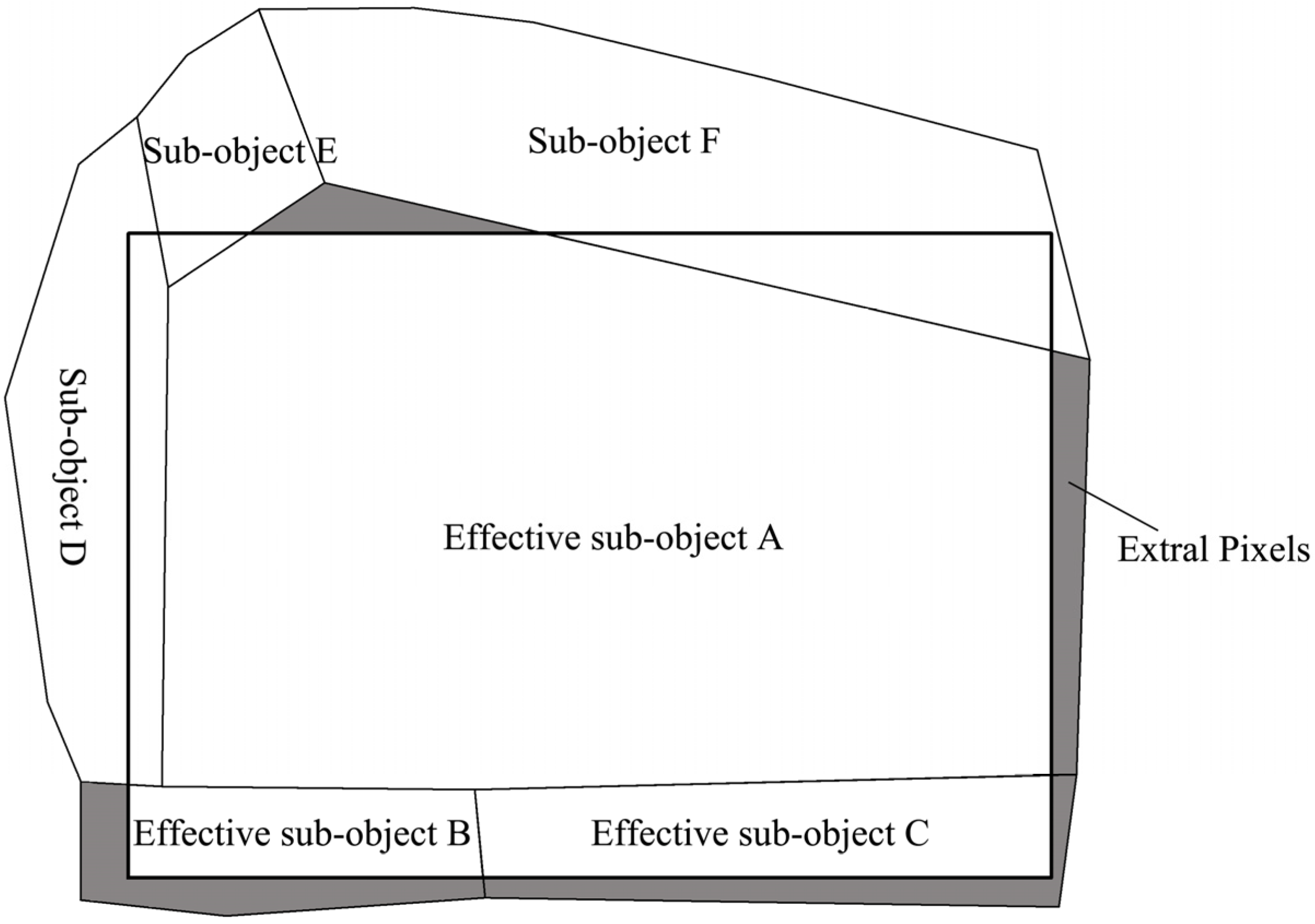
3.3. Minor Object Elimination

After the above steps are performed, minor object elimination is conducted by merging the minor objects, whose sizes are smaller than a threshold, with their most similar neighboring object.

3.4. Quantitative Assessment Method

An empirical discrepancy method [31,45], which uses manually identified regions as reference objects, was adopted to quantitatively assess segmentation quality. First, clearly separable areas were manually segmented as the reference objects. Then, over-segmentation and under-segmentation were evaluated by two criteria, the AFI [46] and the EPR [31].

The AFI is defined as follows:

$$AFI=\frac{A_{refer}-A_{largest}}{A_{refer}}$$

(16)

where A_refer and A_largest, are, respectively, the areas of the reference object and the largest segment within it. A larger AFI value corresponds to more over-segmentation of the object.

To understand EPR, we need to introduce the term effective sub-object, which represents objects “consisting of more than 55 percent of the pixels from the reference area” [31]. The extra pixels are those pixels included in the effective sub-objects but not included in the reference area. The definition of an effective sub-object and extra pixels are illustrated in Figure 5. The bold black rectangle is the reference area which includes 6 sub-objects. Other polygons are the sub-objects of the reference area, which are produced by segmentation. Sub-object A, B and C are effective sub-objects and the gray areas are the extra pixels.

Figure 5. A schematic representation of segmentation illustrating “effective sub-objects” and “extra pixels”. The bold black rectangle is the reference area which includes 6 sub-objects. Sub-object A, B and C are effective sub-objects and the gray areas are the extra pixels.

Figure 5. A schematic representation of segmentation illustrating “effective sub-objects” and “extra pixels”. The bold black rectangle is the reference area which includes 6 sub-objects. Sub-object A, B and C are effective sub-objects and the gray areas are the extra pixels.

The EPR is defined as follows:

$$EPR=\frac{A_{extra}}{A_{refer}}$$

(17)

where A_extra is the area of extra pixels and A_refer is the areas of the reference object. EPR indicates the degree of under-segmentation. A larger EPR value corresponds to more under-segmentation of the object. In special cases, no effective sub-object exists, or the area of effective sub-objects in the reference area is too small (less than 55 percent of the reference area in this research). In this situation, we set the EPR to 1, which means that the object is completely under-segmented.

In this research, an object is considered over-segmented if the AFI of the object is greater than a given threshold (we used 0.25 as an empirical number in this research). In contrast, when the EPR of an object is greater than a threshold (also 0.25 in this research), the object is considered under-segmented. An objects is regarded as being well-segmented when its EPR and AFI are both smaller than 0.25. The rates of over-, under- and well-segmented objects are used to assess the accuracy. To assess its performance on objects of varied sizes, all the objects are divided into 3 groups, including small, medium and large objects. The rates of over-, under- and well-segmented objects are calculated for each of these 3 groups.

4. Results and Discussion

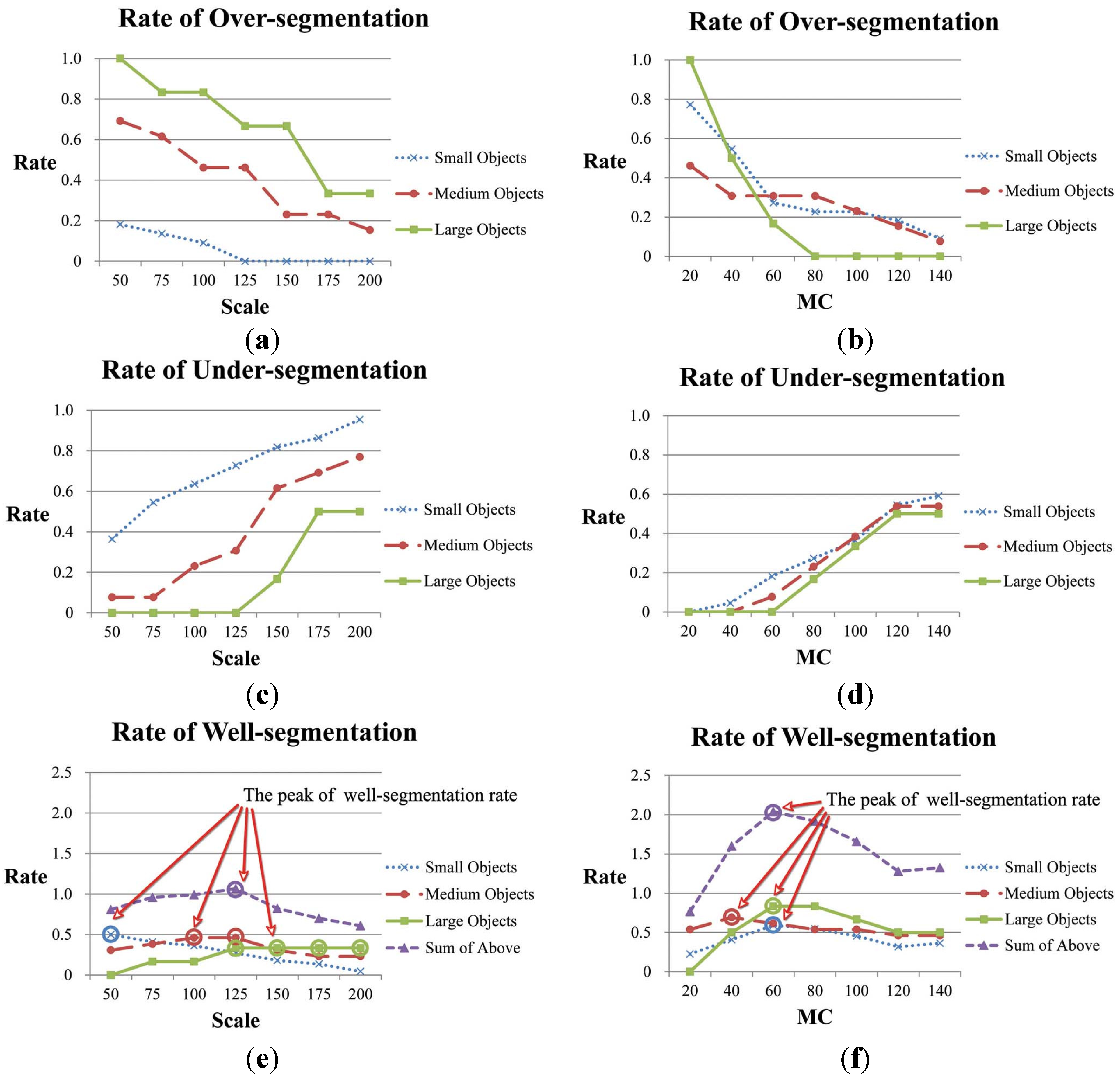
4.1. The Effect of Algorithm Parameters

In the proposed method, five parameters control the quality of the final segments: the initial segmentation scale, T (the constraining threshold for the object size in CSVD), ε (the control variable in the EP), the scale parameter of MC for region merging, and lastly the minimum object size in the minor object elimination process. Since minor object elimination is a simple process, the effect of the minimum object size on the segmentation results was not evaluated.

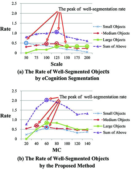
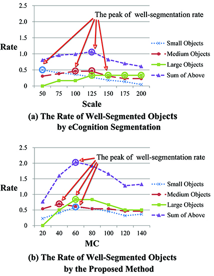
4.1.1. Scale of Initial Segmentation

Different SVD thresholds were tested as initial segmentation scales for all three study areas. Since the initial segmentation results were similar, R1 is used as an example for analysis. In Figure 6a, a threshold of 10 was used, and the image was partitioned into 202,608 segments. Figure 6c shows a zoomed-in area of (a). The pixels in the same object have similar values. When the threshold reached 50 (see Figure 6b,d), each object becomes less homogenous and the number of objects dramatically decreases to 22,043.

Generally, smaller scales produce segments with higher homogeneity but results in too many partitions (over-segmentation), which may increase the computing time in subsequent steps. In contrast, larger scales generate fewer segments but lead to under-segmentation of particular objects, which cannot be fixed by the subsequent region-merging process. Consequently, a reasonable threshold must be chosen to strike a balance between segmentation quality and processing speed. Our experiments used SVD thresholds for the scale of initial segmentation between 20 and 30, which determined on trials and error using the test images. For the initial segmentation, a small scale is preferred because over-segmentation is allowed in this stage.

Figure 6. Initial segments of R1. (a) Threshold of 10 with 202,608 objects. (b) Threshold of 50 with 22,043 objects. Images (c,d) are zoomed-in area of (a,b), respectively.

Figure 6. Initial segments of R1. (a) Threshold of 10 with 202,608 objects. (b) Threshold of 50 with 22,043 objects. Images (c,d) are zoomed-in area of (a,b), respectively.

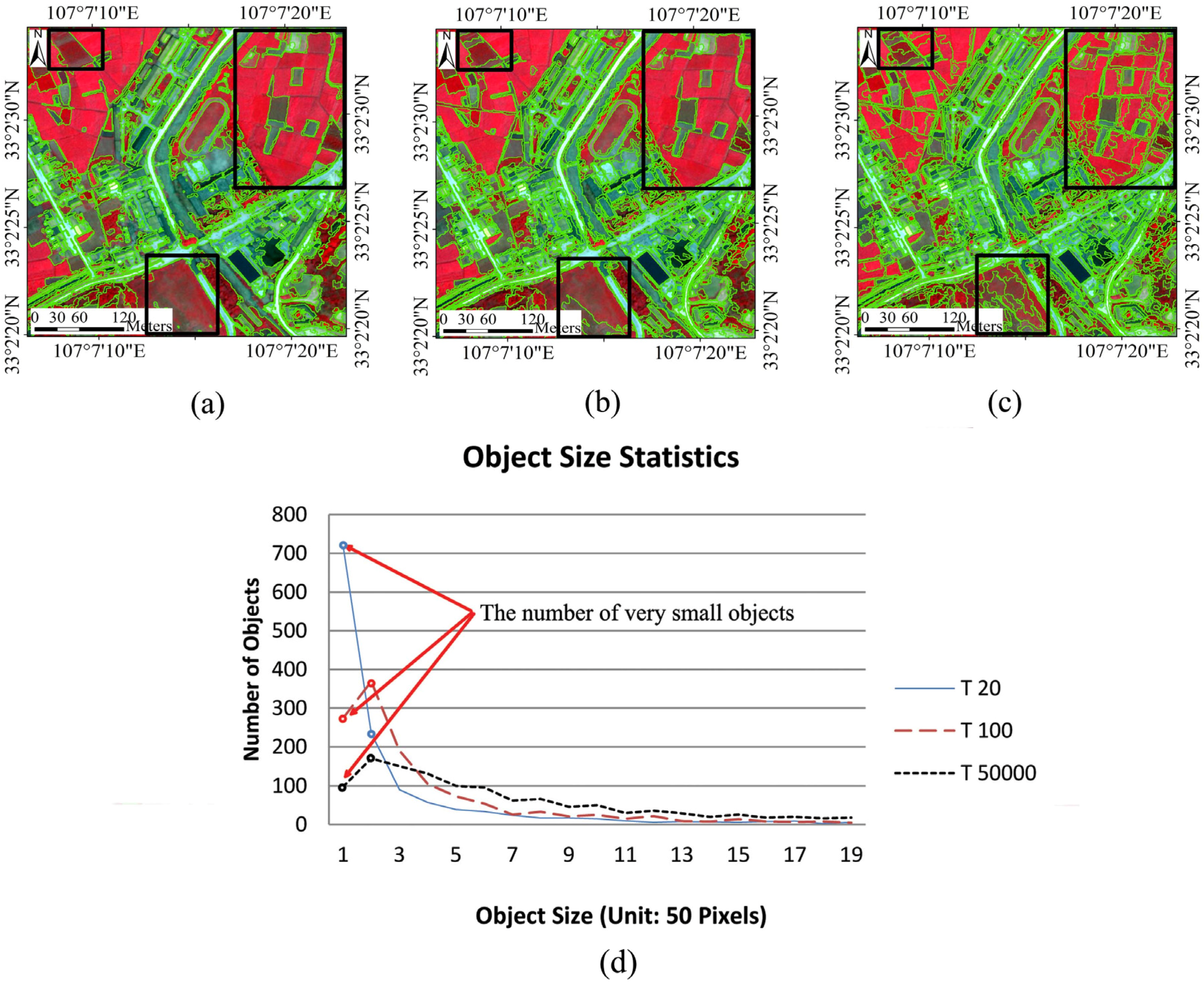
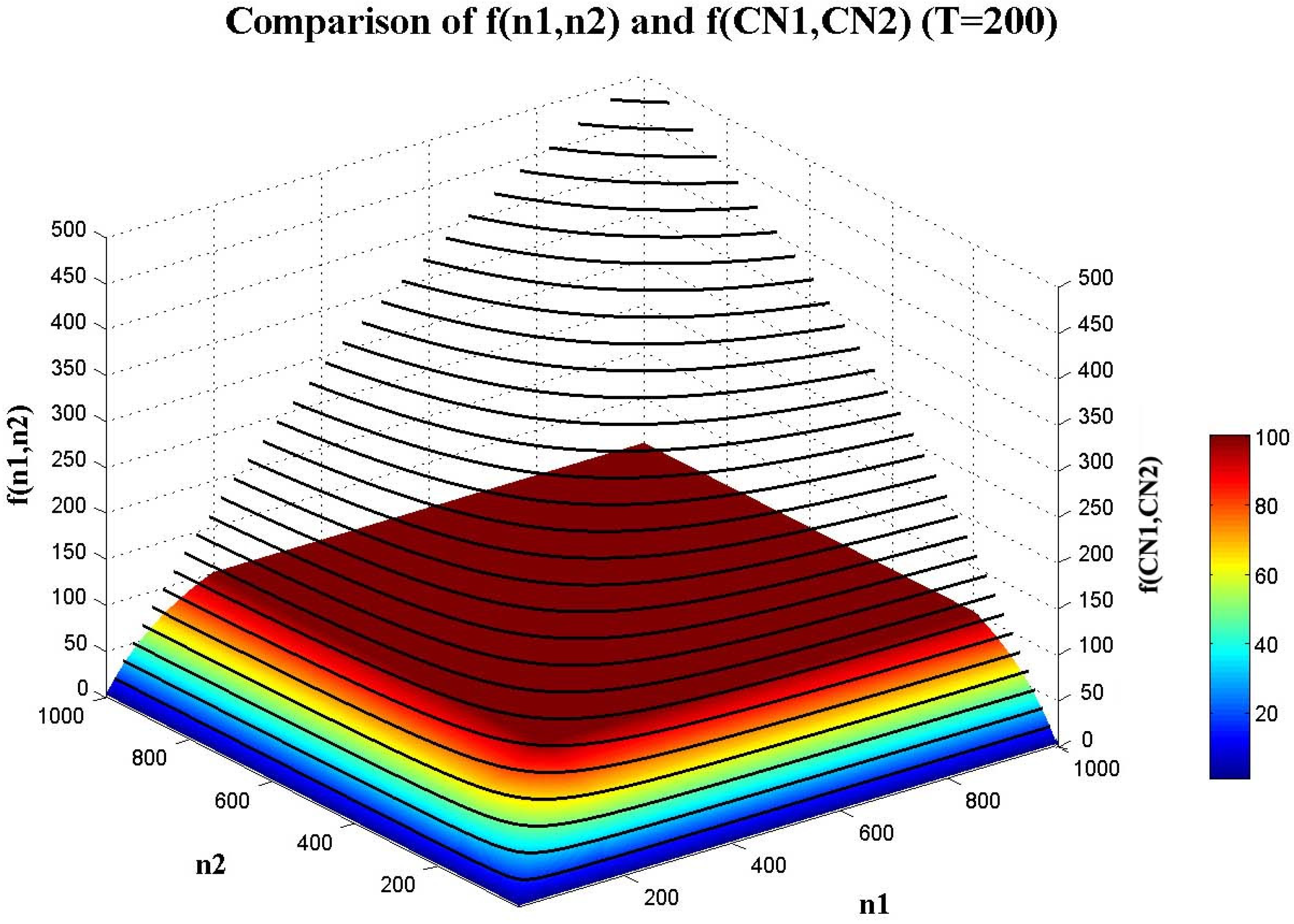
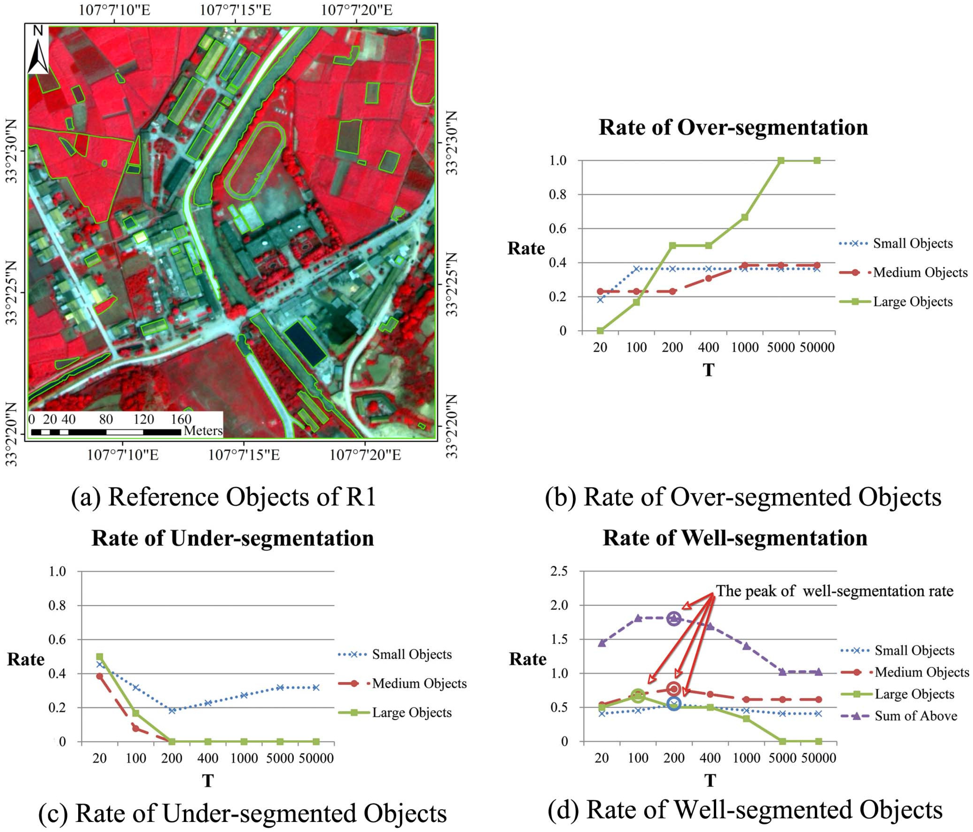
4.1.2. The Constraining Threshold for Object Size in CSVD: T

Different T values of 20, 100 and 50,000 were tested in R1, all other parameters remaining the same with initial scale set to 20 and ε to 0. The results are shown in Figure 7a–c, respectively. All three tests partitioned the image into 1400 segments. The influence of T can be seen in two aspects.

First, large objects tend to merge with their neighbor objects when T is smaller. In Figure 7a, a very small T (20) caused the large objects within the upper-left rectangle to become under-segmented; when T was increased to 100 (Figure 7b), segmentation improved. Different types of farmland with different spectral values were separated, and over-segmentation did not occur. When T was further increased to 50,000 (Figure 7c), this area became over-segmented. Similar outcomes can be observed in the other two rectangles in Figure 7. As T increased, the areas in the two rectangles became increasingly more fragmented. For large objects, a small T can keep them integrated, but too small a T may cause particular large objects to be under-segmented. It is worth mentioning that when T was set as 50,000, CSVD was equivalent to SVD, because the largest object in Figure 7c has a size of 11,071 pixels.

Second, a smaller T, on the other hand, can also better preserve small objects. Figure 7d is a graph showing statistics for the number of objects with sizes smaller than 1000 pixels in Figure 7a–c. In Figure 7d, when T was set to the very small value of 20, approximately 900 objects had sizes smaller than 100 pixels. Among these 900 objects, approximately 700 were smaller than 50 pixels, most of which were noise or minor objects that can be ignored. When T was increased to 100 and 50,000, the number of objects smaller than 100 pixels drastically decreased to approximately 600 and 300, including 300 and 100 objects smaller than 50 pixels, respectively. Therefore, a small T helps maintain small objects; however, a T that is too small will produce too many minor objects and noise.

Figure 7. The influence of T in constrained spectral variance difference (CSVD). Images (a–c) are the segmentation results of R1. All three tests feature an initial scale of 20, an ε of 0 and 1400 segments. However, in (a–c), T was set to 20, 100 and 50,000, respectively. Panel (d) is a statistical graph of the number of objects with sizes smaller than 1000 pixels in (a–c).

Figure 7. The influence of T in constrained spectral variance difference (CSVD). Images (a–c) are the segmentation results of R1. All three tests feature an initial scale of 20, an ε of 0 and 1400 segments. However, in (a–c), T was set to 20, 100 and 50,000, respectively. Panel (d) is a statistical graph of the number of objects with sizes smaller than 1000 pixels in (a–c).

To better assess the effect of T, quantitative assessment was performed on different segmentation results generated by different T values, including 20, 100, 200, 400, 800, 5000 and 50,000, and other parameters were kept the same with those in Figure 7. Figure 8a shows the reference data of R1, which include 22 small objects (100–999 pixels), 13 medium size objects (1000–4999 pixels) and 6 large objects (more than 5000 pixels). Figure 8b–d displays the plots of over-, under- and well-segmentation rate, respectively. In Figure 8b, all the over-segmentation rates of small, medium and large objects increase with T. That is because a larger T value makes the f(CN₁,CN₂) between large objects and their neighbor greater, and thus results in higher priority for small objects to be merged, especially those smaller than 100 pixels. When T was further increased over 800, the rate of over-segmentation for small objects showed a slight decrease, because some of the originally over-segmented small objects became well-segmented or under-segmented. In Figure 8c, when T was set to 20, all objects in the 3 size groups were seriously under-segmented because a large number of minor objects were generated with such a small T (Figure 7d). Since the total number of objects was kept to 1400, the numbers of small, medium, objects resulted were less than they should be due to the number of objects were used up by minor objects. When T was increased to 100 and 200, the number of minor objects sharply decreased (Figure 7d). As a result, the rates of under-segmentation decreased for all object types. However, when T was increased to be larger than 200, some of the small objects were merged to their neighbors and became under-segmented. Figure 8d shows the well-segmentation rates of small, medium, large objects and, additionally their sums. These rates reached their peaks when T was set to 100 or 200.

Figure 8. (a) The reference objects of R1, including 22 small objects (100–999 pixels), 13 medium size objects (1000–4999 pixels) and 6 large objects (more than 5000 pixels); (b–d) display the rates of over-segmented, under-segmented and well-segmented objects, respectively.

Figure 8. (a) The reference objects of R1, including 22 small objects (100–999 pixels), 13 medium size objects (1000–4999 pixels) and 6 large objects (more than 5000 pixels); (b–d) display the rates of over-segmented, under-segmented and well-segmented objects, respectively.

4.1.3. The Edge Penalty Control Variable ε

An experiment was also performed with different ε values to evaluate the effects of the EP on segmentation. In this test, the initial scale and T were set to 20 and 300, respectively, and the number of segments was forced to 360. Figure 9a–c show the results when ε was set to 0, 0.1 and 0.5, respectively. When ε was set to 0, i.e., no EP was included in the merging process (Figure 9a), the CSVD was able to generate an acceptable result, particularly for objects with obvious spectral value differences. Therefore, CSVD alone had the ability to produce good segmentation results. However, inaccurate boundaries appeared between some objects that didn’t have perceptible spectral difference along their common boundary. When ε was set to 0.1 (Figure 9b), particular object pairs without clearly defined boundaries merged. This merging is especially obvious in the northern vegetated area. In contrast, many buildings with high edge strength in the settlement area remained partitioned. Figure 9d–f show the zoomed-in areas of Figure 9a–c. In the white rectangles (Figure 9d,e), the boundary accuracy is significantly improved through the use of the EP. Within the black rectangle of Figure 9f, the edge strength between the farmland and its neighboring vegetated area was not very high. When the edge penalty was given the higher weight of 0.5, the farmland was merged with its neighboring object, although the average spectral difference between the two objects was evident. Therefore, a ε value that is too large may introduce undesired under-segmentation.

Figure 9. The influence of edge penalty. Images (a–c) are segmentation results of R3. All three tests feature an initial scale of 20, a T of 300 and 360 segments. Only ε varies and was set to 0, 0.1 and 0.5 in (a–c), respectively. (d–f) are zoomed-in areas of (a–c), respectively.

Figure 9. The influence of edge penalty. Images (a–c) are segmentation results of R3. All three tests feature an initial scale of 20, a T of 300 and 360 segments. Only ε varies and was set to 0, 0.1 and 0.5 in (a–c), respectively. (d–f) are zoomed-in areas of (a–c), respectively.

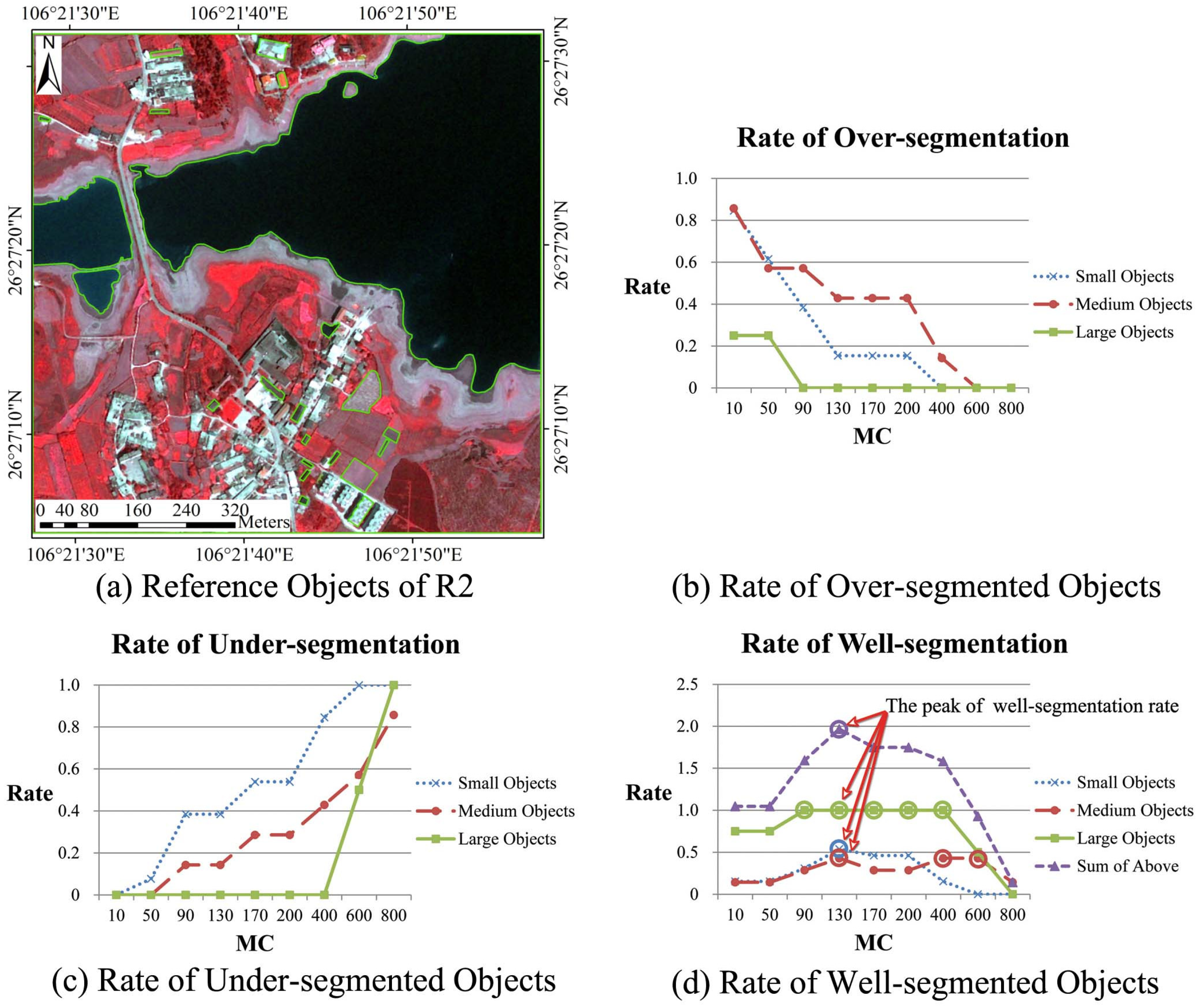
4.1.4. The Scale Parameter for MC

In this test, different MC thresholds that represented segmentation scale parameters were tested on R2, and the results are shown in Figure 10. The MC scale parameter was set to 30, 130 and 200 in Figure 10a–c respectively. The other parameters (initial scale, ε, and T) remained the same, and were set to 20, 0.1 and 300 respectively. To illustrate more detail in the results, Figure 10d–f show zoomed-in areas of Figure 10a–c. The MC scale parameter of 10 partitioned the image into 1213 fragments (Figure 10a,d). The objects with minor spectral differences were separated (note the farmland in Figure 10d). When the MC was increased to 130 (Figure 10b,e), the objects with similar spectral values were merged. When the MC reached 200 (Figure 10c,f), more objects were merged, and only those with a significant spectral difference from their neighbors were preserved.

Figure 10. The influence of different MC values. All three tests set initial scale to 20, T to 300, and ε to 0.1. Only MC varied and was set to 30, 130 and 200 in (a–c), respectively. Images (d–f) are zoomed-in areas of (a–c), respectively.

Figure 10. The influence of different MC values. All three tests set initial scale to 20, T to 300, and ε to 0.1. Only MC varied and was set to 30, 130 and 200 in (a–c), respectively. Images (d–f) are zoomed-in areas of (a–c), respectively.

Like Section 4.1.2, a group of segmentation results were generated by different MC values ranged from 10 to 800, and other parameters remained the same with those in Figure 10. Figure 11a shows the reference data of R2, which include 13 small objects (100–399 pixels), 7 medium size objects (400–1999 pixels) and 4 large objects (more than 2000 pixels). Figure 11b–d display the plots of over-, under- and well-segmentation rate, respectively. With the increasing of MC value, more and more objects were merged. Therefore, their over-segmentation rates decreased (Figure 11b) while their under-segmentation rates increased (Figure 11c). Figure 11d shows the well-segmentation rates of small, medium, large objects and their sums. It can be seen that all the 3 groups of objects were best-segmented (highest well-segmentation rate) when the same MC value of 130 is used.

Figure 11. Quantitative assessment results by different MC values in R2. (a) is the reference objects of R2, including 13 small objects (100–399 pixels), 7 medium size objects (400–1999 pixels) and 4 large objects (more than 2000 pixels); (b–d) display the rates of over-segmented, under-segmented and well-segmented, respectively.

Figure 11. Quantitative assessment results by different MC values in R2. (a) is the reference objects of R2, including 13 small objects (100–399 pixels), 7 medium size objects (400–1999 pixels) and 4 large objects (more than 2000 pixels); (b–d) display the rates of over-segmented, under-segmented and well-segmented, respectively.

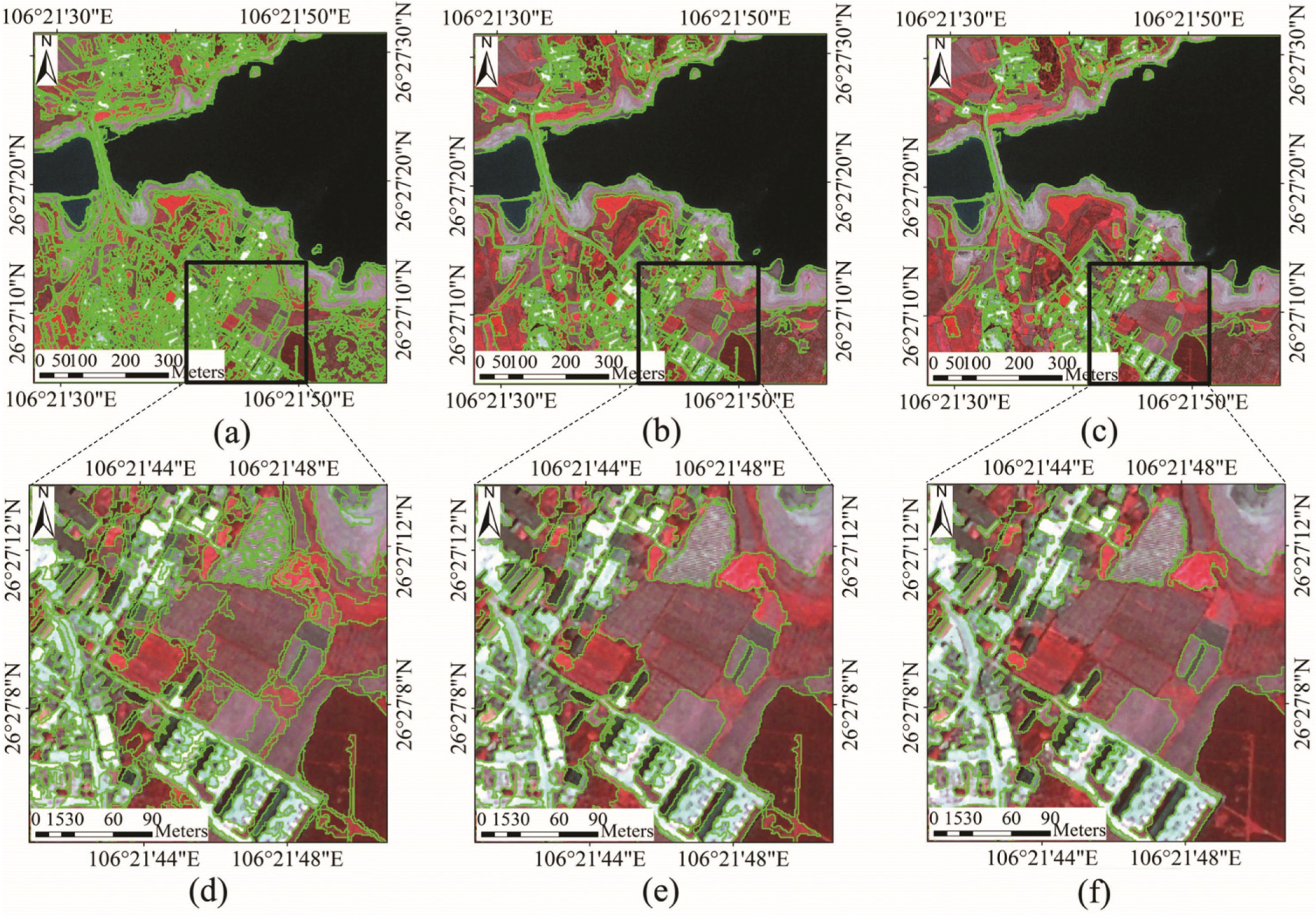
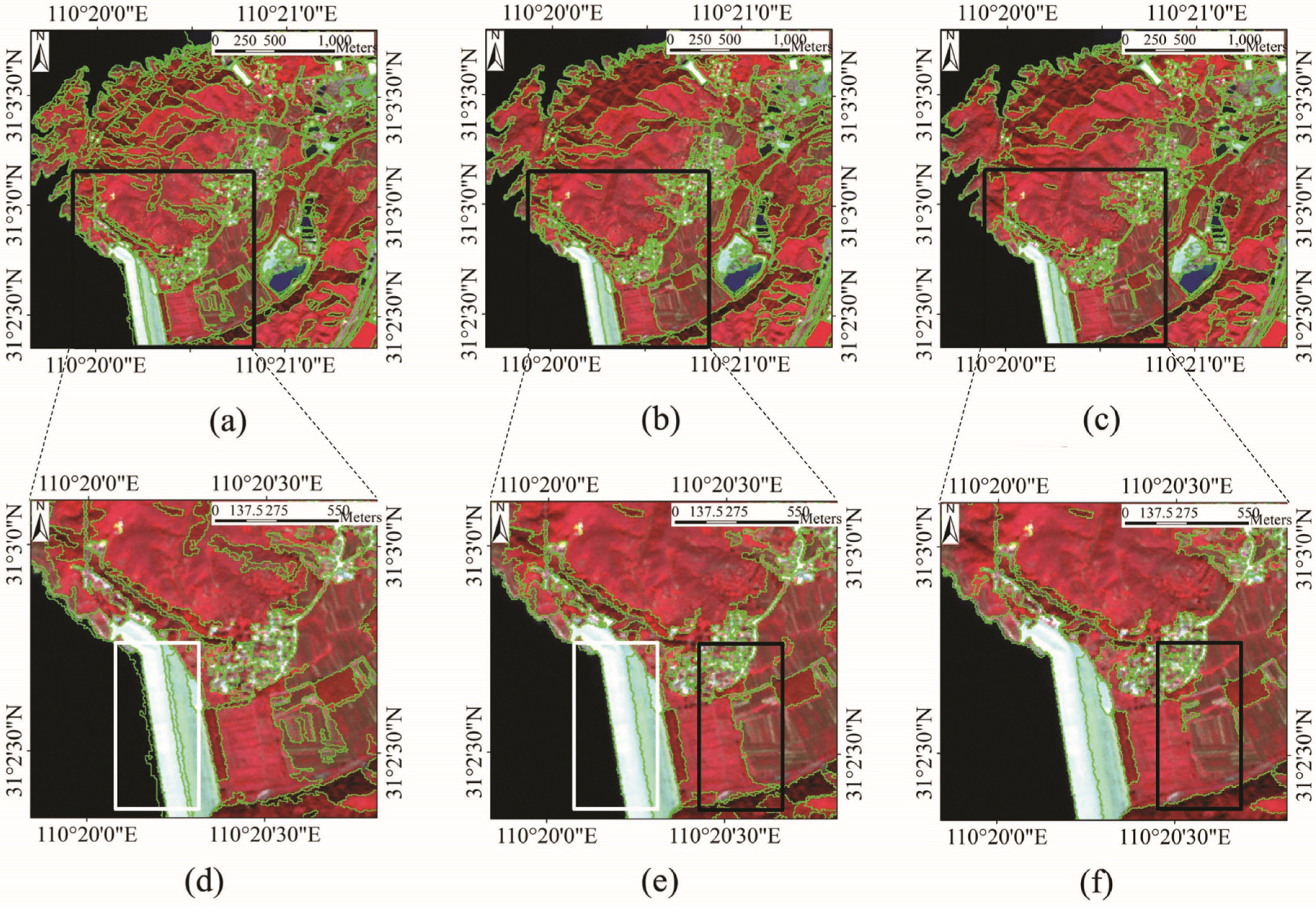
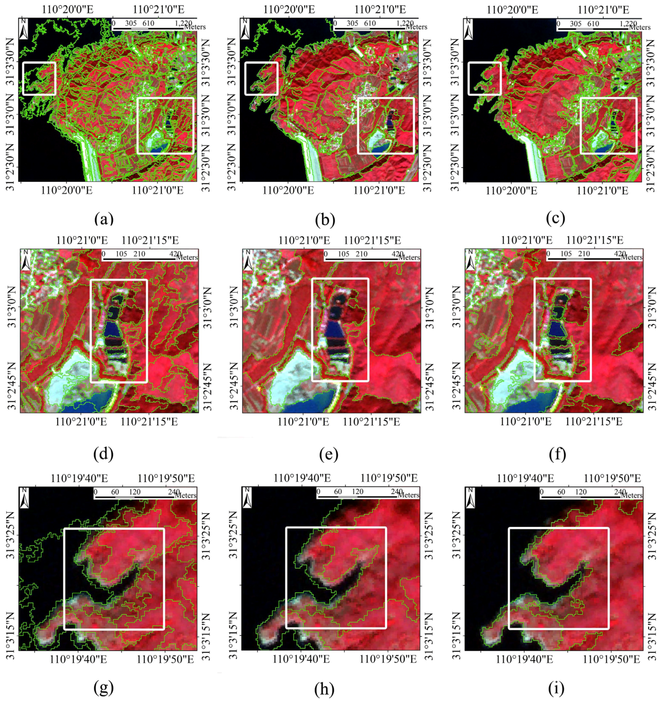
4.2. Comparison with eCognition Software Segmentation

eCognition is one of the most widely used commercial OBIA software in remote sensing. The multi-resolution segmentation algorithm in eCognition employs the local mutual best-fitting strategy and uses spectral and shape heterogeneity differences as merging criteria. For spectral heterogeneity, the eCognition segmentation applied a SVD-based criterion [22]. For shape heterogeneity, the eCognition segmentation used compactness and smoothness. In the proposed algorithm, shape heterogeneity could also be incorporated into the merging criterion to make objects compact and smooth. However, this could also jeopardize boundary accuracy [28] and fragment some elongated objects. Since this research focuses primarily on the improvement of spectral heterogeneity differences, the shape weight parameters for eCognition and our algorithm were both set to 0 for our comparison tests.

Figure 12 shows the results of the two algorithms applied to R3. Figure 12a,b are the results of eCognition segmentation with the MC scale parameter set to 200 and 700, respectively. Figure 12d–h are two zoomed-in areas of Figure 12a,b. In Figure 12a, the upper-left reservoir (black area) was over-segmented but the pools in the rectangle of (d) were correctly segmented. When the scale parameter was increased to 700, the pools became under-segmented, and the reservoir remained over-segmented (see Figure 12b,e). Therefore, it is impossible to simultaneously segment both the reservoir and the pools correctly using a single scale parameter in eCognition. However, this was not a problem for our algorithm. Figure 12c shows our segmentation results with ε, T and the MC scale parameter set to 0.1, 100 and 55, respectively. Figure 12f,i are the zoomed-in areas of Figure 12c. The proposed method is able to correctly segment both medium and large size objects, while also preserving the small objects. The eCognition segmentation also generated incorrect merges when the scale parameter was raised to 700. In Figure 12h, a small portion of the water body was incorrectly merged with the bank by eCognition, whereas the proposed algorithm correctly segments the entire water body (Figure 12i). Consequently, the incorporation of EP improved the accuracy of boundary delineation.

Figure 12. Comparison of the proposed algorithm and eCognition segmentation applied to R3. Images (a,b) are the results of the eCognition segmentation with scale parameters set to 200 and 700, respectively. Image (c) is the result of the proposed segmentation with ε, T and MC set to 0.1, 100 and 55, respectively. Images (d–f) show a zoomed-in area of (a–c). Images (g–i) show another zoomed-in area of (a–c). Their corresponding areas are showed in the white rectangles in (a–c).

Figure 12. Comparison of the proposed algorithm and eCognition segmentation applied to R3. Images (a,b) are the results of the eCognition segmentation with scale parameters set to 200 and 700, respectively. Image (c) is the result of the proposed segmentation with ε, T and MC set to 0.1, 100 and 55, respectively. Images (d–f) show a zoomed-in area of (a–c). Images (g–i) show another zoomed-in area of (a–c). Their corresponding areas are showed in the white rectangles in (a–c).

For quantitative comparison, the same assessment method used in Section 4.1 was employed. Because the quantitative evaluation of R1, R2 and R3 are similar, we only show the results of R1 here. The reference objects are the same with those used in Section 4.1.2. Figure 13a,c,e display the plots of over-, under- and well-segmentation rate of the eCognition segmentation results using different scales. For comparison, the corresponding plots of the segmentation results generated by the proposed algorithm with different MC scales were showed in Figure 13b,d,f. Other parameters (initial scale, ε, and T) remained the same, and were set to 20, 0.1 and 100 respectively. Since both eCognition segmentation and the proposed algorithm are region-merging methods, their over-segmentation rates decrease with the increase of scale parameter (Figure 13a,b). However, their difference is also obvious. In eCognition segmentation, the over-segmentation rate of larger objects is always greater than that of smaller objects (Figure 13a). Similar phenomenon can also be found for the under-segmentation rate (Figure 13c,d). This is because the f(n₁,n₂) in SVD of smaller objects is smaller, which gives smaller objects higher priority to be merged, while larger objects are prone to be over-segmented. Figure 13e shows the well-segmentation rates of eCognition segmentation. It can be seen that the well-segmentation rate of small objects get its highest value when the scale parameter is small, i.e., 50. Whereas, the well-segmentation rates of the medium and large objects need a higher scale parameter to reach their peaks. Therefore, it is impossible for eCognition segmentation to partition small-, medium- and large-sized objects well simultaneously by using one scale parameter. However, the proposed algorithm can strike good balance among varied-size objects by one scale parameter (around 60). When the MC scale parameter of the proposed algorithm was set to 60, the well-segmentation rate of each group objects is also much higher than the highest = well-segmentation rate of eCognition segmentation. For example, the well-segmentation rate of medium objects by scale 60 using the proposed algorithm (Figure 13f) is about 0.62, which is higher than that in eCognition segmentation by any scale (highest rate is 0.46).

The most significant difference between our method and other algorithms is that we used CSVD instead of SVD for MC. The CSVD reduces the influence of object size in the merging process compared with the SVD. In SVD-based algorithms, the MC of large objects pairs with similar spectral values can be enormous, because the corresponding f(n₁,n₂) can be very large. In CSVD, the influence of f(n₁,n₂) is constrained. The MC of large objects pairs with similar spectral values can be limited to a small value, thus merging can still be conducted on these objects pairs. Therefore, the proposed algorithm can prevent large objects from being over-segmented. Likewise, the MC of small objects pairs with distinct spectral differences can also be large enough to prevent them from being merged. Additionally, the introduction of an EP, if properly weighted, also improves the accuracy of object boundaries, although an over-weighted edge penalty may jeopardized the merging process.

In our experiments, the parameter of minimum object size for minor objects elimination was set to small values (20–50). It was observed that these values of the parameter barely had any influence on the final results. A minimum object size parameter that is too large should be avoided because they may jeopardize the segmentation accuracy.

Compared to SVD based method such as eCognition segmentation, the proposed algorithm only involves two extra steps (the calculation of CN and EP), which didn’t increase much computational complexity. For example, in a speed test using R2, the proposed method took 6.63 second to partition R2 into 4800 segments, which cost only 0.99 second more than that of the pure SVD based method.

Figure 13. Quantitative assessment results by different MC values in R2. Plots on the left side of the figure display the over-, under- and well-segmentation rate of eCognition segmentation using different scale parameters. The corresponding plots of the proposed method are displayed on the right part. (a) Rate of over-segmented objects by eCognition segmentation; (b) Rate of over-segmented objects by the proposed method; (c) Rate of under-segmented objects by eCognition segmentation; (d) Rate of under-segmented objects by the proposed method; (e) Rate of well-segmented objects by eCognition segmentation; (f) Rate of well-segmented objects by the proposed method.

Figure 13. Quantitative assessment results by different MC values in R2. Plots on the left side of the figure display the over-, under- and well-segmentation rate of eCognition segmentation using different scale parameters. The corresponding plots of the proposed method are displayed on the right part. (a) Rate of over-segmented objects by eCognition segmentation; (b) Rate of over-segmented objects by the proposed method; (c) Rate of under-segmented objects by eCognition segmentation; (d) Rate of under-segmented objects by the proposed method; (e) Rate of well-segmented objects by eCognition segmentation; (f) Rate of well-segmented objects by the proposed method.

In the proposed method, five parameters must be set manually. While it is also a common challenge that most commercial segmentation software such as eCognition, and ENVI are facing, because these parameters are often data dependent. However, ideally image segmentation software should provide the automatic configuration and optimization of the parameters and this will be significant part of our future research. Additionally, because the top-to-bottom and left-to-right fast scan method for initial segmentation is relatively simple, a small initial scale is needed to achieve a good accuracy. Unfortunately, a small initial scale leads to excessive initial segments, which substantially increases the computational burden. Therefore, a superior initial segmentation method may be explored in further research.

5. Conclusions

This research proposes a new algorithm for image segmentation. The goal of the proposed method was to generate objects of varied size which are close to their real-world counterparts in a single scale layer. We introduced constrained spectral variance difference (CSVD) and Edge Penalty (EP) to generate Merging Criterion (MC), and adopted a global mutual best-fitting strategy implemented through region adjacent graphs (RAG) and nearest neighbor graphs (NNG) to achieve this objective.

The significant novelty of the proposed algorithm is the devise of CSVD, which largely reduce the influence of size. Based on both visual and quantitative evaluations, we demonstrated that the proposed algorithm was able to segment the objects properly regardless of their size. When compared with results from the commercial eCognition software, the proposed method better preserves the entirety of large objects, while also prevents small objects from mingling with other objects. It can strike a good balance when partitioning varied-size objects using one MC scale parameter. Additionally, in a quantitative comparison, the highest sum of the well-segmentation rate of small-, medium- and large-sized objects using the proposed algorithm reached 2.04 which was much higher than that of the eCognition segmentation (1.07) using one scale parameter. Besides, the proposed method improved the accuracy of boundary delineation. Finally, compared to a pure SVD based method, the proposed algorithm incurs less than 20 percent extra computational burden.

References

1. Cracknell, A.P. Synergy in remote sensing—What’s in a pixel? Int. J. Remote Sens. 1998, 19, 2025–2047. [Google Scholar]
2. Blaschke, T.; Strobl, J. What’s wrong with pixels? Some recent developments interfacing remote sensing and GIS. GeoBIT/GIS 2001, 6, 12–17. [Google Scholar]
3. Burnett, C.; Blaschke, T. A multi-scale segmentation/object relationship modelling methodology for landscape analysis. Ecol. Model. 2003, 168, 233–249. [Google Scholar] [CrossRef]
4. Hay, G.J.; Castilla, G. Geographic Object-Based Image Analysis (GEOBIA): A new name for a new discipline. In Object Based Image Analysis: Spatial Concepts for Knowledge-Driven Remote Sensing Applications; 1st ed.; Blaschke, T., Lang, S., Hay, G., Eds.; Springer: Heidelberg/Berlin, Germany; New York, NY, USA, 2008; pp. 93–112. [Google Scholar]
5. Blaschke, T. Object based image analysis for remote sensing. ISPRS J. Photogramm. Remote Sens. 2010, 63, 2–16. [Google Scholar] [CrossRef]
6. Haralick, R.M.; Shapiro, L. Survey: Image segmentation techniques. Comput. Vis. Graph. Image Process. 1985, 29, 100–132. [Google Scholar] [CrossRef]
7. Pal, R.; Pal, K. A review on image segmentation techniques. Pattern Recognit. 1993, 26, 1277–1294. [Google Scholar] [CrossRef]
8. Blaschke, T.; Burnett, C.; Pekkarinen, A. New contextual approaches using image segmentation for object-based classification. In Remote Sensing Image Analysis: Including the Spatial Domain, 1st ed.; de Meer, F., de Jong, S., Eds.; Kluver Academic Publishers: Dordrecht, The Netherland, 2004; Volume 5, pp. 211–236. [Google Scholar]
9. Reed, T.R.; Buf, J.M.H.D. A review of recent texture segmentation and feature extraction techniques. Comput. Vis. Graph. Image Process. 1993, 57, 359–372. [Google Scholar] [CrossRef]
10. Schiewe, J. Segmentation of high-resolution remotely sensed data- concepts, applications and problems. Int. Arch. Photogramm. Remote Sens. Spat. Inf. Sci. 2002, 34, 380–385. [Google Scholar]
11. Dey, V.; Zhang, Y.; Zhong, M. A review on image segmentation techniques with remote sensing perspective. In Proceedings of the ISPRS TC VII Symposium—100 Years ISPRS, Vienna, Austria, 5–7 July 2010; Wagner, W., Székely, B., Eds.; ISPRS: Vienna, Austria, 2010. [Google Scholar]
12. Gonçalves, H.; Gonçalves, J.A.; Corte-Real, L. HAIRIS: A method for automatic image registration through histogram-based image segmentation. IEEE Trans. Image Process. 2011, 20, 776–789. [Google Scholar] [CrossRef] [PubMed]
13. Cocquerez, J.P.; Philipp, S. Analyse D’images: Filtrage et Segmentation; Masson: Paris, France, 1995; p. 457. [Google Scholar]
14. Vincent, L.; Soille, P. Watershed in digital spaces: An efficient algorithm based on immersion simulations. IEEE Trans. Pattern Anal. Mach. Intell. 1991, 13, 583–598. [Google Scholar] [CrossRef]
15. Debeir, O. Segmentation Supervisée d’Images. Ph.D. Thesis, Faculté des Sciences Appliquées, Université Libre de Bruxelles, Brussels, Belgium, 2001. [Google Scholar]
16. Canny, J. A computational approach to edge detection. IEEE Trans. Pattern Anal. Mach. Intell. 1986, 6, 679–698. [Google Scholar] [CrossRef]
17. Carleer, A.P.; Debeir, O.; Wolff, E. Assessment of very high spatial resolution satellite image segmentations. Photogramm. Eng. Remote Sens. 2005, 71, 1285–1294. [Google Scholar] [CrossRef]
18. Jain, A.K. Fundamentals of Digital Image Processing; Prentice-Hall: Upper Saddle River, NJ, USA, 1989; pp. 347–356. [Google Scholar]
19. Wang, D. A multiscale gradient algorithm for image segmentation using watersheds. Pattern Recognit. 1997, 30, 2043–2052. [Google Scholar] [CrossRef]
20. Horowitz, S.L.; Pavlidis, T. Picture segmentation by a tree traversal algorithm. J. ACM 1976, 23, 368–388. [Google Scholar] [CrossRef]
21. Adams, R.; Bischof, L. Seeded Region Growing. IEEE Trans. Pattern Anal. Mach. Intell. 1994, 16, 641–647. [Google Scholar] [CrossRef]
22. Baatz, M.; Schäpe, M. Multiresolution segmentation—An optimization approach for high quality multi-scale image segmentation. In Angewandte Geographische Informations-Verarbeitung XII, Beiträge zum AGIT-Symposium Salzbug, Salzbug, Austria; Strobl, J., Blaschke, T., Griesebner, G., Eds.; Herbert Wichmann Verlag: Karlsruhe, Germany, 2000; pp. 12–23. [Google Scholar]
23. Pavlidis, T.; Liow, Y.T. Integrating region growing and edge detection. IEEE Trans. Pattern Anal. Mach. Intell. 1990, 12, 225–233. [Google Scholar] [CrossRef]
24. Cortez, D.; Nunes, P.; Sequeira, M.M.; Pereira, F. Image segmentation towards new image representation methods. Signal Process. 1995, 6, 485–498. [Google Scholar]
25. Haris, K.; Efstratiadis, S.N.; Maglaveras, N.; Katsaggelos, A.K. Hybrid image segmentation using watersheds and fast region merging. IEEE Trans. Image Process. 1998, 7, 1684–1699. [Google Scholar] [CrossRef] [PubMed]
26. Castilla, G.; Hay, G.J.; Ruiz, J.R. Size-constrained region merging (SCRM): An automated delineation tool for assisted photointerpretation. Photogramm. Eng. Remote Sens. 2008, 74, 409–419. [Google Scholar] [CrossRef]
27. Yu, Q.; Clausi, D.A. IRGS: Image segmentation using edge penalties and region growing. IEEE Trans. Pattern Anal. Mach. Intell. 2008, 30, 2126–2139. [Google Scholar] [CrossRef] [PubMed]
28. Zhang, X.; Xiao, P.; Song, X.; She, J. Boundary-constrained multi-scale segmentation method for remote sensing images. ISPRS J. Photogramm. Remote Sens. 2013, 78, 15–25. [Google Scholar] [CrossRef]
29. Zhang, X.; Xiao, P.; Feng, X. Fast hierarchical segmentation of high-resolution remote sensing image with adaptive edge penalty. Photogramm. Eng. Remote Sens. 2014, 80, 71–80. [Google Scholar] [CrossRef]
30. Robinson, D.J.; Redding, N.J.; Crisp, D.J. Implementation of a fast algorithm for segmenting SAR imagery. In Scientific and Technical Report; Defense Science and Technology Organization: Canberra, Australia, 2002. [Google Scholar]
31. Marpu, P.R.; Neubert, M.; Herold, H.; Niemeyer, I. Enhanced evaluation of image segmentation results. J. Spat. Sci. 2010, 55, 55–68. [Google Scholar] [CrossRef]
32. Benz, U.C.; Hofmann, P.; Willhauck, G.; Lingenfelder, I.; Heynen, M. Multiresolution, object-oriented fuzzy analysis of remote sensing data for GIS-ready information. ISPRS J. Photogramm. Remote Sens. 2004, 58, 239–258. [Google Scholar] [CrossRef]
33. Beaulieu, J.M.; Goldberg, M. Hierarchy in picture segmentation: A stepwise optimization approach. IEEE Trans. Pattern Anal. Mach. Intell. 1989, 11, 150–163. [Google Scholar] [CrossRef]
34. Saarinen, K. Color image segmentation by a watershed algorithm and region adjacency graph processing. In Proceedings of the IEEE International Conference on Image Processing, Austin, TX, USA, 13–16 November 1994; Volume 3, pp. 1021–1025.
35. Chen, Z.; Zhao, Z.M.; Yan, D.M.; Chen, R.X. Multi-scale segmentation of the high resolution remote sensing image. In Proceedings of the 2005 IEEE International Geoscience and Remote Sensing Symposium, 2005, (IGARSS’05), Seoul, South Korea, 29 July 2005; Volume 5, pp. 3682–3684.
36. Tan, Y.M.; Huai, J.Z.; Tan, Z.S. Edge-guided segmentation method for multiscale and high resolution remote sensing image. J. Infrared Millim. Waves 2010, 29, 312–316. [Google Scholar]
37. Deng, F.L.; Tang, P.; Liu, Y.; Yang, C.J. Automated hierarchical segmentation of high-resolution remote sensing imagery with introduced relaxation factors. J. Remote Sens. 2013, 17, 1492–1499. [Google Scholar]
38. Ballard, D.; Brown, C. Computer Vision, 1st ed.; Prentice-Hall: Englewood Cliffs, NJ, USA, 1982; pp. 159–164. [Google Scholar]
39. Wu, X. Adaptive split-and-merge segmentation based on piecewise least-square approximation. IEEE Trans. Pattern Anal. Mach. Intell. 1993, 15, 808–815. [Google Scholar]
40. Kanungo, T.; Dom, B.; Niblack, W.; Steele, D. A fast algorithm for MDL-based multi-band image segmentation. In Proceedings of the IEEE Computer Society Conference on Computer Vision and Pattern Recognition, Seattle, WA, USA, 21–23 June 1994; pp. 609–616.
41. Luo, J.B.; Guo, C.E. Perceptual grouping of segmented regions in color images. Pattern Recognit. 2003, 36, 2781–2792. [Google Scholar] [CrossRef]
42. Tupin, F.; Roux, M. Markov random field on region adjacency graph for the fusion of SAR and optical data in radar grammetric applications. IEEE Trans. Geosci. Remote Sens. 2005, 43, 1920–1928. [Google Scholar] [CrossRef]
43. Xiao, P.; Feng, X.Z.; Wang, P.; Ye, S.; Wu, G.; Wang, K.; Feng, X.L. High Resolution Remote Sensing Image Segmentation and Information Extraction, 1st ed.; Science Press: Beijing, China, 2012; pp. 167–168. [Google Scholar]
44. Sarkar, A.; Biswas, M.K.; Sharma, K.M. A simple unsupervised MRF model based image segmentation approach. IEEE Trans. Image Process. 2000, 9, 801–812. [Google Scholar] [CrossRef] [PubMed]
45. Zhang, Y.J. A survey on evaluation methods for image segmentation. Pattern Recognit. 1996, 29, 1335–1346. [Google Scholar] [CrossRef]
46. Lucieer, A. Uncertainties in Segmentation and Their Visualization. Ph.D. Thesis, Utrecht University, Utrecht, The Netherlands, 2004. [Google Scholar]