
Ship Detection with Spectral Analysis of Synthetic Aperture Radar: A Comparison of New and Well-Known Algorithms

Abstract
:
1. Introduction
- The paper proposes the first comparison of four sub-look detectors exploiting a large dataset composed of TerraSAR-X, RADARSAT-2 and ALOS-PALSAR (with diversity in frequency, polarization channels and incidence angles).
2. Spectral Analysis of SAR Data
- Sub-looking in the range: In this case, the stability of the targets is tested with respect to variations of frequency. This is due to the fact that, after removal of windowing, the spectrum pixels in range contain the backscattering values when the frequency of the chirp is varied. An ideal point target and (generally) corner reflectors have a response that stays coherent when changing the frequency slightly. By definition, this is the reason why such targets can be focused as single points in an SAR image [34,37].
- Sub-looking in the azimuth (or Doppler): The stability of targets is now tested when they are observed by different angles in the azimuth footprint of the SAR acquisition (i.e., looking fore or aft). Again, a theoretical point target is perfectly isotropic, while static corners mostly stay coherent (even though their amplitude can change significantly along the synthetic antenna). Unfortunately, the Doppler analysis becomes more complicated when the targets are not stationary. Targets that move along the range direction have a different Doppler history compared with static targets. This circumstance has two main effects: firstly, the zero Doppler will be located in a different position, translating the target along the azimuth direction; secondly, the focusing cannot be done optimally (since the Doppler history does not match the reference one), which means that the target will present smearing (i.e., de-focusing). In the framework of ship detection, smearing leads to not having a point target anymore, and therefore, a coherent detector may fail. As a final remark, the Doppler analysis may be performed keeping in mind the possibility of miss detections due to vessel movements [37,38].

3. Target Detectors with Spectral Analysis
3.1. Sub-Look Coherence
3.2. Sub-Look Cross-Correlation
3.3. Sub-Look Entropy
3.4. GLRT
4. Methodology Employed for the Algorithm Comparison
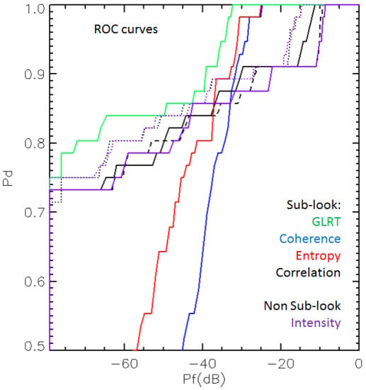
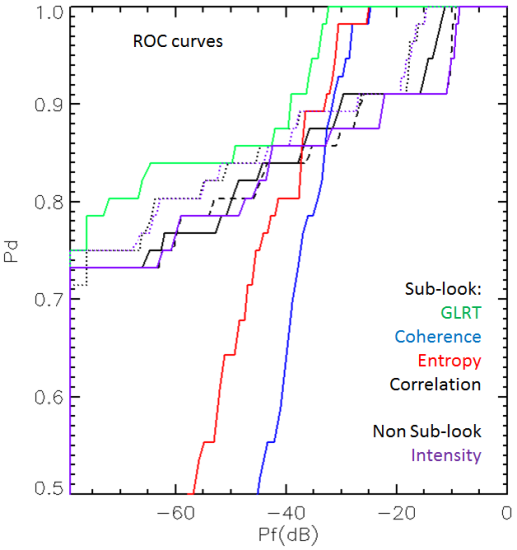
4.1. Receiver Operating Characteristic Curves
4.1.1. Computation of Pd
4.1.2. Computation of Pf
4.2. Detector Parameters
- The first one is related to the process of splitting the image spectrum: the number of sub-images and their overlap in frequency.
- The second one corresponds to the size of windows for eventual boxcar filtering. In this work, the window size of the boxcar filter is never squared, since the resolution in the ground range and azimuth are not the same. In addition, it is assumed that vessels do not have preferential orientations in the horizontal plane (direction of travel).

| Detector | ♯ Sub-Images | Band Overlap |
|---|---|---|
| GLRT | 30 | 96% |
| Entropy | 3 | 50% |
| Correlation | 2 | 0% or 50% |
| Coherence | 2 | 0% |
| Intensity | None | None |
| Detector | RADARSAT-2 (Range × Azimuth) Pixels | TerraSAR-X (Range × Azimuth) Pixels | ALOS-PALSAR (Range × Azimuth) Pixels |
|---|---|---|---|
| GLRT | None | None | None |
| Entropy | (5 × 9) or (3 × 5) | (13 × 5) or (7 × 3) | (3 × 15) or (5 × 25) |
| Correlation | (5 × 9) or (3 × 5) | (13 × 5) or (7 × 3) | (3 × 15) or (5 × 25) |
| Coherence | (5 × 9) or (3 × 5) | (13 × 5) or (7 × 3) | (3 × 15) or (5 × 25) |
| Intensity | None or (5 × 9) or (3 × 5) | None or (13 × 5) or (7 × 3) | None or (3 × 15) or (5 × 25) |
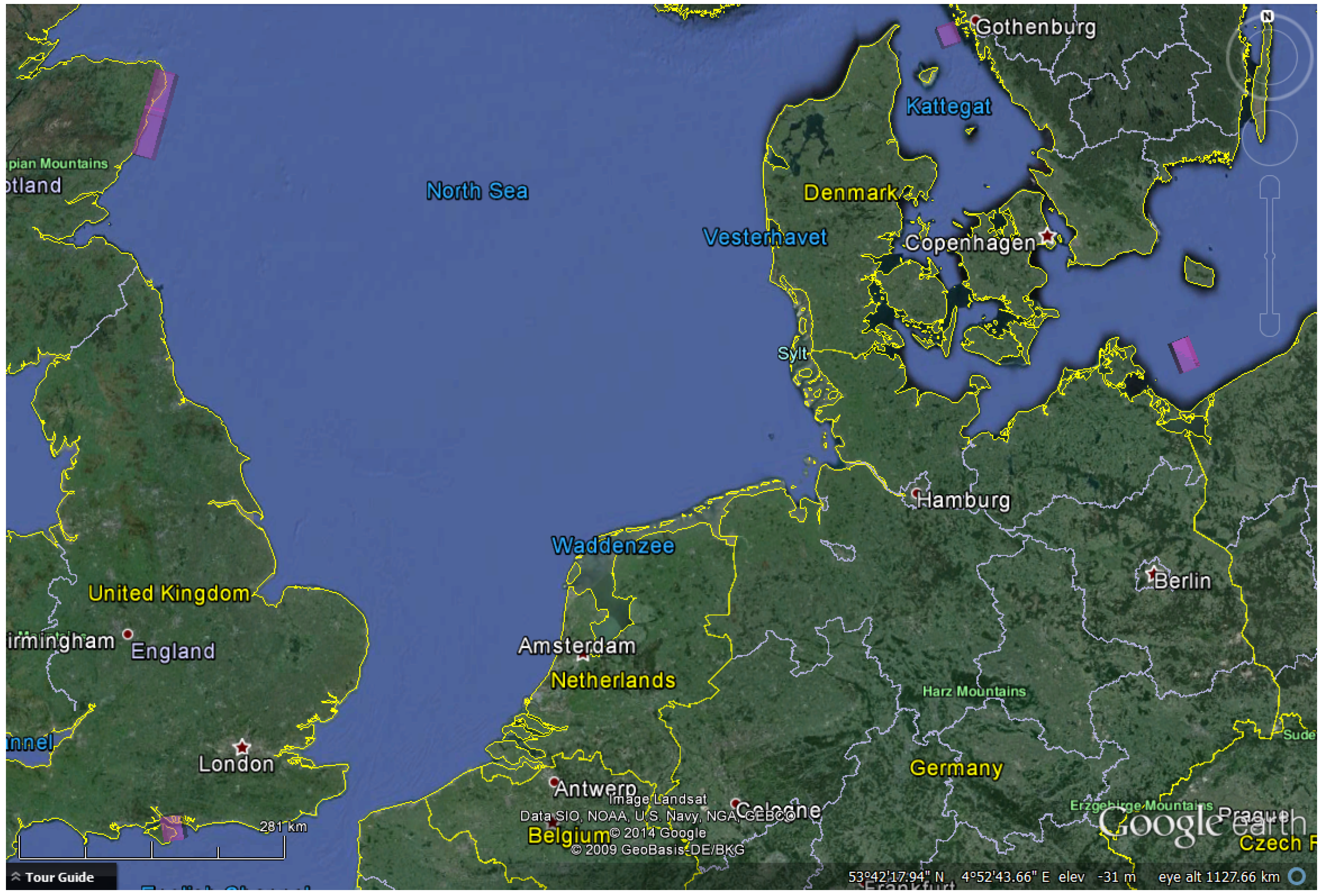
5. Experimental Data
5.1. RADARSAT-2

| Date (Time) | Location | Beam | Incidence Angle | Ground Range Res. | Wind Speed (m/s) | Ships with AIS |
|---|---|---|---|---|---|---|
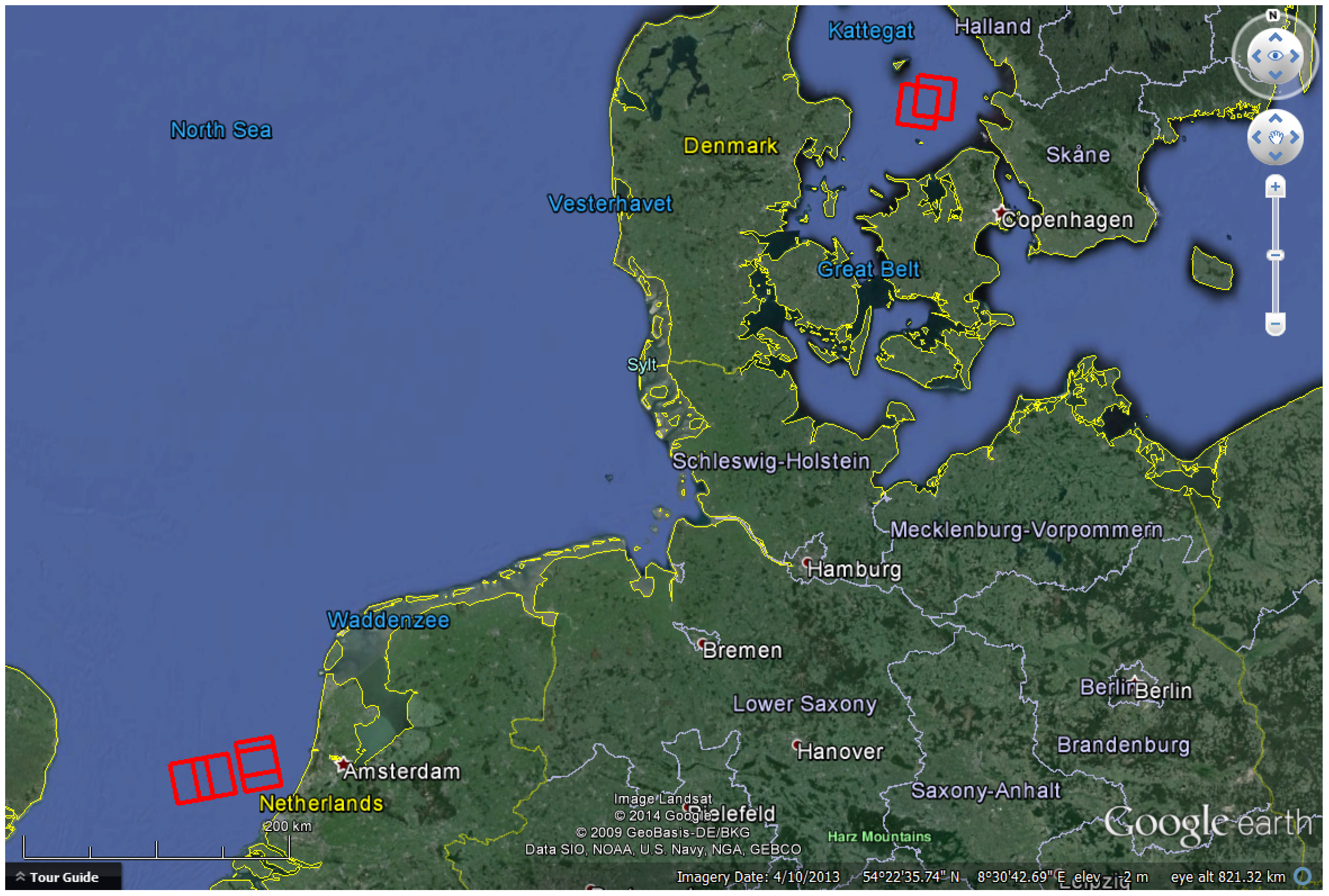
| 29 November 2013 (17:30) | North Sea | FQ12 | ∼ 32° | 10.0 m to 9.5 m | 16.5 (NW) | 12 |
| 3 December 2013 (05:48) | Kattegat | FQ3 | ∼ 21.5° | 14.6 m to 13.4 m | 10.8 (SW) | 6 |
| 23 December 2013 (17:30) | North Sea | FQ13 | ∼ 34° | 9.7 m to 9.3 m | 18.5 (S) | 13 |
| 10 December 2013 (05:43) | Kattegat | FQ6 | ∼ 25° | 13.1 m to 12.2 m | 6.7 (SW) | 9 |
| 16 January 2014 (17:30) | North Sea | FQ15 | ∼ 35° | 9.2 m to 8.8 m | 9.8 (S) | 9 |
| 9 February 2014 (17:30) | North Sea | FQ15 | ∼ 35° | 9.2 m to 8.8 m | 18 (SW) | 20 |
5.2. TerraSAR-X
| Date (Time) | Location | Beam | Incidence Angle | Ground Range Res. | Wind Speed (m/s) | Ships with AIS |
|---|---|---|---|---|---|---|
| 03 December 2012 (06:33) | Aberdeen | stripFar_008 | ∼ 33.5° | 2.1 m | 6.7 (SE) | 16 |
| 11 December 2012 (16:36) | Baltic Sea | stripFar_005 | ∼ 27° | 2.6 m | 11.8 (N) | 8 |
| 05 December 2013 (16:45) | Goteborg | stripFar_006 | ∼ 29° | 2.4 m | Not Recorded | 6 |
| 18 December 2013 (17:45) | Portsmouth | stripNear_007 | ∼ 30° | 2.3 m | Not Recorded | 7 |
| 29 December 2013 (17:45) | Portsmouth | stripNear_007 | ∼ 30° | 2.3 m | Not Recorded | 12 |
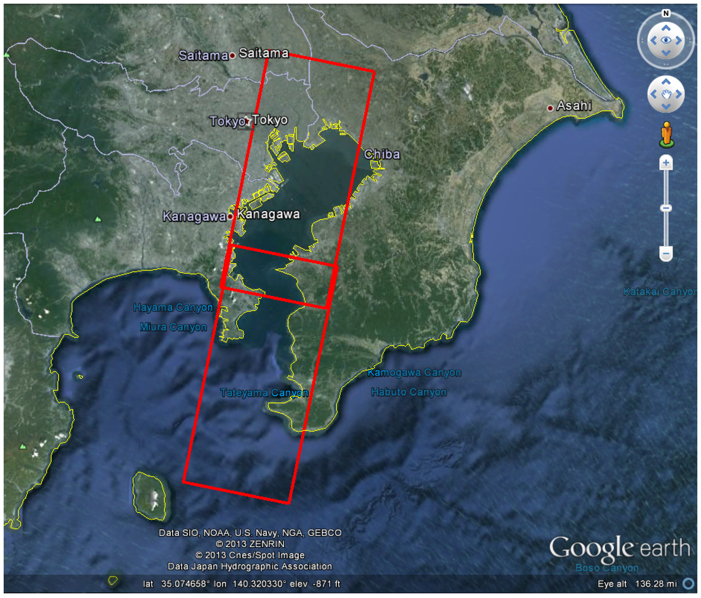
5.3. ALOS-POLSAR

6. Detectors Comparison
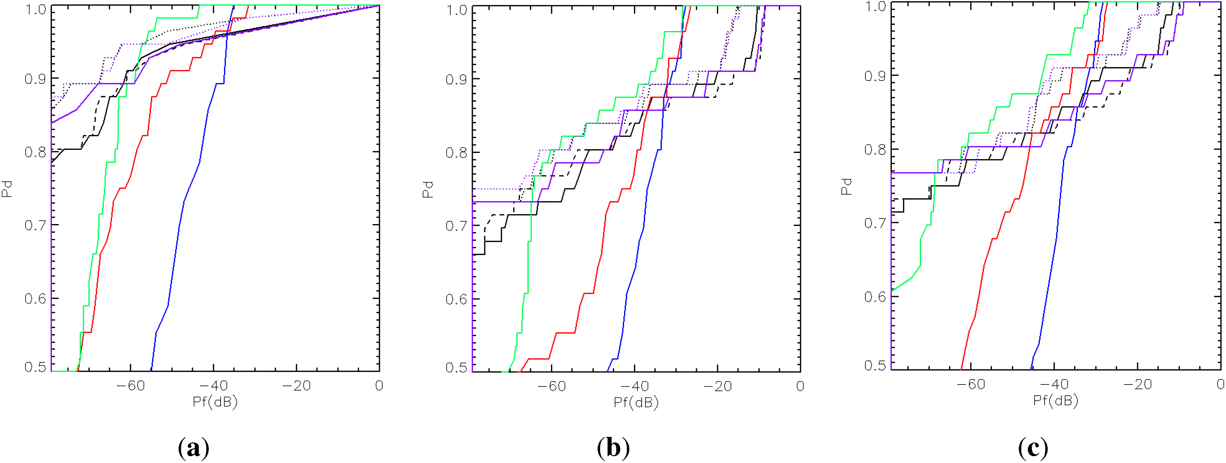
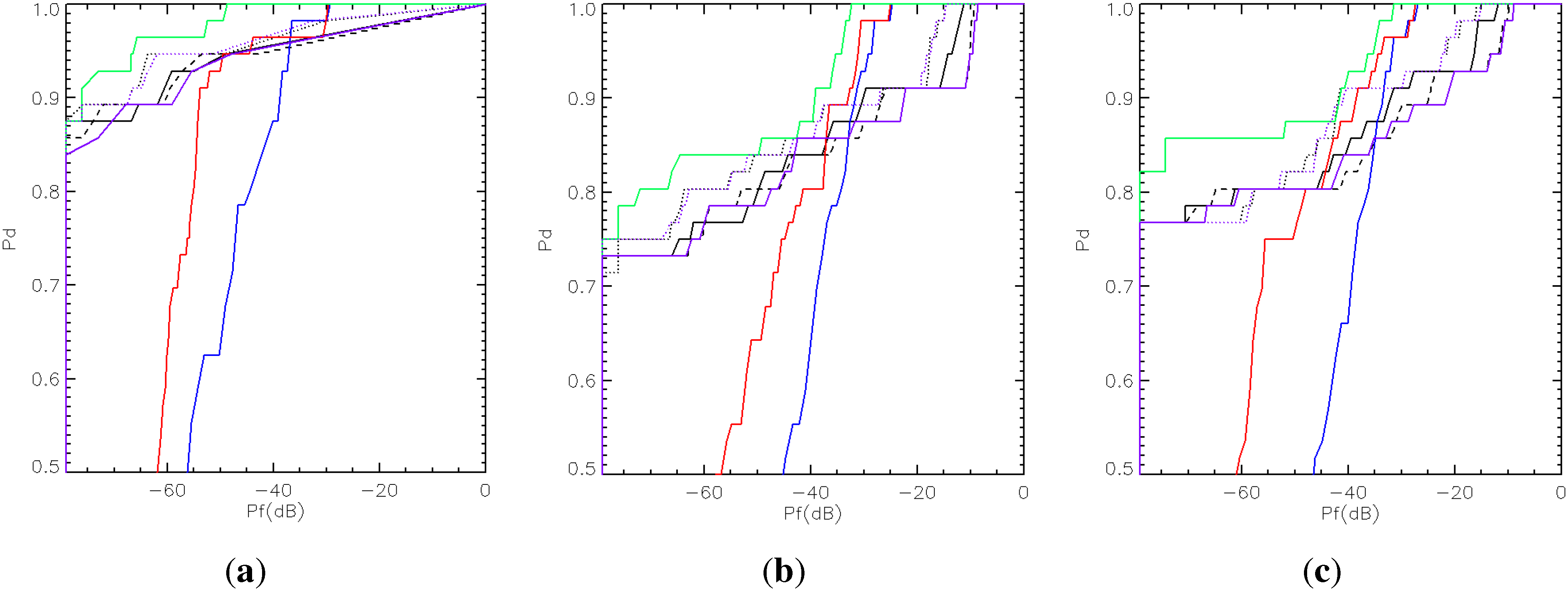
6.1. Comparison with RADARSAT-2 Data
6.1.1. Sub-Look Processing in the Range
6.1.2. Sub-Look Processing in the Azimuth

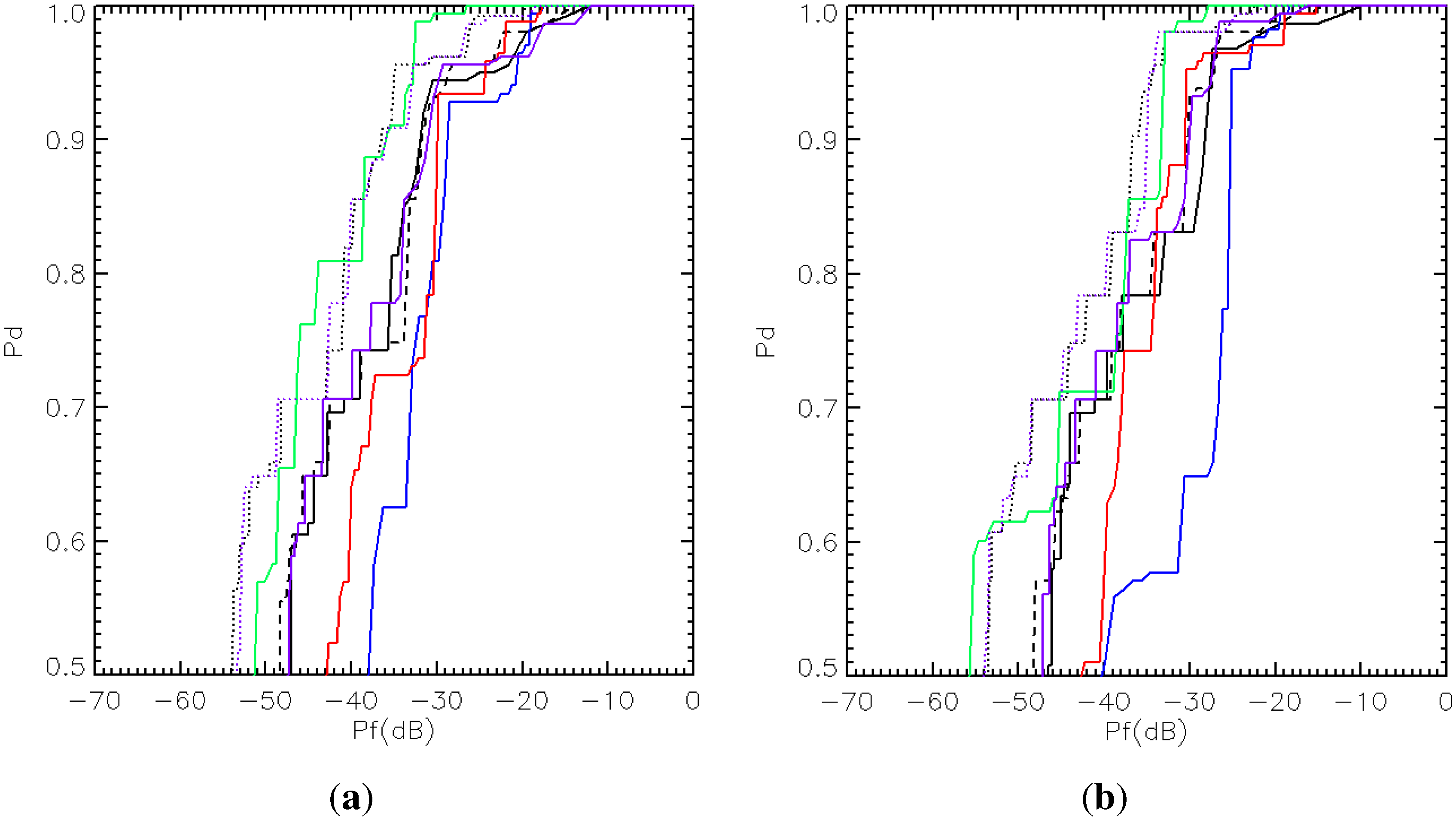
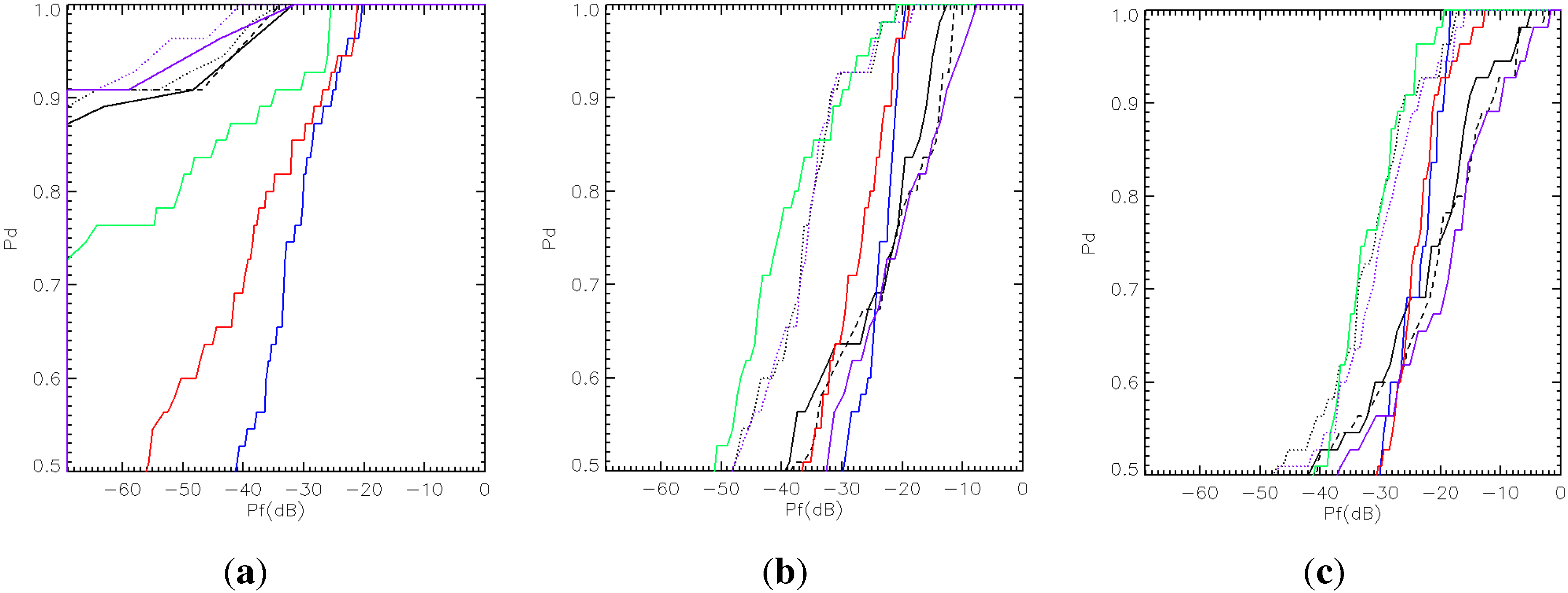
6.2. Comparison with TerraSAR-X Data
6.2.1. Sub-Look Processing in the Range

6.2.2. Sub-Look Processing in Azimuth
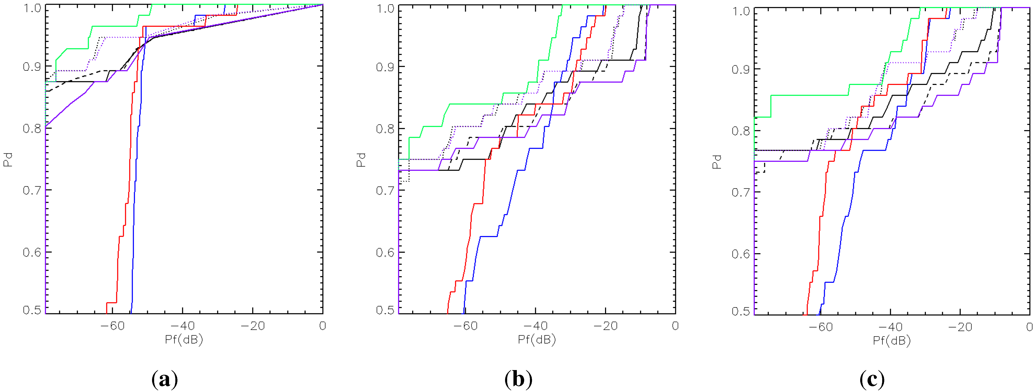
6.3. Comparison with ALOS-PALSAR Data
6.3.1. Sub-Look Processing in the Range
6.3.2. Sub-Look Processing in the Azimuth
7. Discussions
- Polarization channels: The images acquired for the comparison consider different polarization channels. RADARSAT-2 and ALOS-PALSAR are both quad polarimetric, while TerraSAR-X is HH/VV dual polarimetric. In the performed test, it seems that the cross-polarization (HV) provides the best ROC curves for all of the experiments. This has been also reported by several researchers [3,40]. Additionally, this result is in line with the assumption that the sea can be modeled as a Bragg surface [9,51], which assumes a null cross-polarization. It has to be considered, as well, that vessels may scatter less in the cross-channel. However, such a reduction is not as large as for the sea, leading to a higher vessel-sea contrast. Certainly, this is mostly evident in situations where sea clutter is strong (as for harsh weather conditions). Regarding the two co-polarization channels (HH and VV), their performance is comparable, but, in some instances, the results for HH seem to be slightly better [45]. Besides the scattering from the sea (which is, on average, stronger in VV compared to HH), this fact may be due to the effect of dihedral scattering (e.g., double-bounce) between sea and vessel, especially if the vessel has one axis oriented along the azimuth direction. Indeed, horizontal dihedral scattering is stronger in the HH channel compared to the VV channel. As a final remark, we could say that the use of the cross-polarization would be preferred, and the importance of sub-look processing will reveal more when the cross-polarization cannot be acquired, because only single-polarimetric data co-polarized channels are available.
- Central frequency and resolution: The possibility of comparing three different SAR systems allows some analysis concerning the frequency providing the best ROC curves. Three frequencies have been exploited, L-, C- and X-band. Clearly, the ROC curves for the different sensors are not utterly comparable, since the images were not acquired at the same time, and the sensors’ resolution and incidence angle are different. Therefore, the following conclusions are only indicative. Firstly, the results obtained with RADARSAT-2 and TerraSAR-X are compared, without considering the cross-polarization channel. From the analysis, it seems that RADARSAT-2 and TerraSAR-X provide similar ROC curves for values of Pd > 0.8, and RADARSAT-2 generally has better ROCs for Pd < 0.8. Even if TerraSAR-X offers a higher resolution (about 2.5 × 6.5 m compared with 5.2 × 10 m of RADARSAT-2), the performance of RADARSAT-2 is as good as the one of TerraSAR-X (or even better for lower values of Pd). An explanation for this could be related to the fact that the sea states captured by the images were particularly high, and sea clutter appears stronger in the X-band. For this reason, if the spatial resolution were the same, the C-band could be advantageous when weather conditions are expected to be rough. Secondly, the ALOS dataset shows a detection performance comparable to the one of RADARSAT-2 in the cross-polarization. Following the previous rationale, the L-band should provide an even lower sea clutter. On the contrary, vessels at the L-band may have a lower backscattering, as well (unless they are very large), and the resolution of ALOS is poorer than RADARSAT-2. These two drawbacks may be causing the lower performance of ALOS at the co-polarization channels.
- Comparison with the intensity detector: The intensity detector is tested in order to understand if the sub-look analysis provides noticeable benefits. In general, such sub-look analysis requires images in the SLC format and not detected by multi-look. In this work, the intensity detector has been also used as a reference for the other algorithms, since it is a well-known and standard method. Looking at the obtained results, the ROC curves clearly show that the sub-look analysis generally provides an improved performance. However, such enhancement is in some situations very small, as for the ALOS cross-polarization. It can be also observed that the main advantages of the sub-look analysis are more evident when the co-polarizations are used and the clutter is stronger. Per contra, in situations where the clutter contribution is low, a simple threshold on the cross-polarization backscattering may be satisfactory.
- Best detector: For our analyses (with the exception of the ALOS cross-polarization), the GLRT detector provides the best ROC curves, even though the improvement on TerraSAR-X data is not very large. The GLRT is the only sub-look detector that does not require spatial averaging (i.e., it works on single pixels), and that is the most likely reason for the better performance. The only loss of resolution experienced by this detector is because of the spectrum splitting (i.e., the generation of the sub-images), which corresponds to 50% in these experiments.
- Dimensions of averaging windows: Speckle filtering is another source of resolution loss, and therefore, it is valuable to consider its effect on the performance. In this work, the boxcar windows are always rectangular and not squared, in order to finally obtain areas on the ground that are approximately squared. For the intensity detector, it can be observed that omitting speckle filtering provides better ROC curves. Therefore, the loss of resolution due to the spatial averaging is not compensated by the reduction of speckle variation. Similarly, if the averaging window of the sub-look coherence or entropy detectors is reduced, their performances improve, even if not very largely. Nevertheless, there is a threshold value for the averaging window size when the performance is optimized and any smaller window returns worse results. In the limit, a window of (1 × 1) pixels produces always Pd = Pf = 1. The reason for this result is that the estimation of these detectors’ outputs is more critical than the one of the intensity detector, and the use of a few pixels provides strongly biased results. Therefore, this counterbalances the improvement of having higher resolution. Likewise, the sub-look correlation has an optimal dimension of the averaging window, but when the window is reduced to (1 × 1) pixels, the obtained ROC becomes very similar to the one of the SLC (unfiltered) intensity. The explanation for this is because the product of the two sub-looks is not completely canceling the sea clutter out, since this may happen only after averaging (the output has the same information content as the intensity image, except for a loss of resolution due to the spectrum splitting and the absence of a square). As a final remark regarding the exploitation of small averaging windows, a minor speckle reduction may have some disadvantages when a statistical test is exploited for setting the detection threshold. This rationale is mostly true if the pdf is well-known. A reduction of variance may have the opposite effect of having a test that sets the threshold very close to the mean, neglecting heavier tails and providing, then, more false alarms than expected.
8. Conclusions
- Initially, two algorithms previously used for the detection of coherent targets on land and natural areas were tested for the first time ever on ship detection. These approaches are the GLRT and the sub-look entropy [6,33]. The sub-look entropy detector allows one to split the spectrum into several sections (also with large overlap), providing that vessels that are not stable in a few sections can still be detected. The GLRT detector, in addition, does not require spatial averaging (apart from the initial sub-looking), and therefore, the resolution is only slightly reduced.
- Secondly, there are no similar studies that compare the same amount of sub-look ship detectors over such a large and variable dataset. The main idea behind this study is to understand if sub-look analysis provides benefits compared with ordinary backscattering analysis. In other words, the benefits of acquiring and exploiting the phase of the SAR image compared to only the detected images is investigated.
Acknowledgments
Author Contributions
Conflicts of Interest
References
- Barele, V.; Gade, M. Remote Sensing of the European Seas; Springer: Berlin, Germany, 2008. [Google Scholar]
- Franceschetti, G.; Lanari, R. Synthetic Aperture Radar Processing; CRC Press: Boca Raton, FL, USA, 1999. [Google Scholar]
- Crisp, D.J. The State-of-the-Art in ship detection in Synthetic Aperture Radar imagery. Available online: http://oai.dtic.mil/oai/oai?verb=getRecord&metadataPrefix=html&identifier=ADA426096 (accessed on 9 April 2015).
- Sanjuan-Ferrer, M.J. Detection of Coherent Scatterers in SAR Data: Algorithms and Applications. Ph.D. Thesis, ETH Zurich, Zurich, Switzerland, 2013. [Google Scholar]
- Sanjuan-Ferrer, M.; Hajnsek, I.; Papathanassiou, K.; Moreira, A. A new detection algorithm for coherent scatterers in SAR data. IEEE Trans. Geosci. Remote Sens. 2015. submitted. [Google Scholar]
- Schneider, R.Z.; Papathanassiou, K.P.; Hajnsek, I.; Moreira, A. Polarimetric and interferometric characterization of coherent scatterers in urban areas. IEEE Trans. Geosci. Remote Sens. 2006, 44, 971–984. [Google Scholar] [CrossRef]
- Arnaud, A. Ship detection by SAR interferometry. In Proceedings of the IEEE 1999 International Geoscience and Remote Sensing Symposium, Hamburg, Germany, 28 June–2 July 1999; Volume 5, pp. 2616–2618.
- Ouchi, K.; Tamaki, S.; Yaguchi, H.; Iehara, M. Ship detection based on coherence images derived from cross correlation of multilook SAR images. IEEE Geosci. Remote Sens. Lett. 2004, 1, 184–187. [Google Scholar] [CrossRef]
- Jackson, C.R.; Apel, J.R. Synthetic Aperture Radar Marine Users Manual; U.S. DEPARTMENT OF COMMERCE, National Oceanic and Atmospheric Administration (NOAA). Available online: http://www.sarusersmanual.com/ (accessed on 23 April 2015).
- Cloude, S.R. Polarisation: Applications in Remote Sensing; Oxford University Press: Oxford, UK, 2009. [Google Scholar]
- Alpers, W. Imaging Ocean Surface Waves by Synthetic Aperture Radar: A Review; Ellis Horwood Ltd.: Cambridge, UK, 1983. [Google Scholar]
- Elfouhaily, T.B.; Chapron, K.K.; Vandemark, D. A unified directional spectrum for long and short wind-driven waves. J. Geophys. Res. 1997, 102, 15781–15796. [Google Scholar] [CrossRef]
- Plant, W.J. Surfaces, Waves and Fluxes: Bragg Scattering of Electromagnetic Waves from the Air/Sea Interface; Kluwer Academic: Dordrecht, The Netherlands, 1990. [Google Scholar]
- Thompson, D.R. Radar Scattering from Modulated Wind Waves: Calculation of Microwave Doppler Spectra from the Ocean Surface with a Time-Dependent Composite Model; Kluwer Academic: Dordrecht, The Netherlands, 1989. [Google Scholar]
- Wackerman, C.; Friedman, K.; Pichel, W.; Clemente-Colon, P.; Li, X. Automatic detection of ships in RADARSAT-1 SAR imagery. Can. J. Remote Sens. 2001, 27, 568–577. [Google Scholar] [CrossRef]
- Brizi, M.; Lombardo, P.; Pastina, D. Exploiting the shadow information to increase the target detection performance in SAR images. In Proceedings of the 5th International Conference on Radar Systems, RADAR’99, Brest, Germany, 17–21 May 1999.
- Campbell, J.; Vachon, P. Optimisation of the Ocean FeaturesWorkstation for ship detection. Canadian Centre of Remote Sensing: Suwanee, GA, USA, 1997. [Google Scholar]
- Marino, A.; Cloude, S.R.; Woodhouse, I.H. A polarimetric target detector using the Huynen Fork. IEEE Trans. Geosci. Remote Sens. 2010, 48, 2357–2366. [Google Scholar] [CrossRef]
- Chapple, P.; Bertilone, D.; Caprari, R.; Newsam, G. Stochastic modelbased processing for detection of small targets in non-Gaussian natural imagery. IEEE Trans. Image Process. 2001, 10, 554–564. [Google Scholar] [CrossRef] [PubMed]
- Conte, E.; Lops, M.; Ricci, G. Asymptotically optimum radar detection in compound-Gaussian clutter. IEEE Trans. Aerospace Electron. Syst. 1995, 31, 617–625. [Google Scholar] [CrossRef]
- Ferrara, G.; Migliaccio, M.; Nunziata, F.; Sorrentino, A. Generalized-K (GK)-based observation of metallic objects at sea in full-resolution Synthetic Aperture Radar (SAR) data: a multipolarization study. IEEE J. Ocean. Eng. 2011, 36, 195–204. [Google Scholar] [CrossRef]
- Friedman, K.; Wackerman, C.; Funk, F.; Pichel, W.; Clemente-Colon, P.; Li, X. Validation of a CFAR vessel detection algorithm using known vessel locations. In Proceedings of the 2001 IEEE International Geoscience and Remote Sensing Symposium (IGARSS’01), Sydney, NSW, Australia, 9–13 July 2001; pp. 1804–1806.
- Johannessen, J. Coastal observing systems: The role of synthetic aperture radar. Johns Hopkins APL Tech. Dig. 2000, 21, 41–48. [Google Scholar]
- Lopes, A.; Nezry, E.; Touzi, R.; Laur, H. Structure detection and statistical adaptive speckle filtering in SAR images. Int. J. Remote Sens. 1993, 14, 1735–1758. [Google Scholar] [CrossRef]
- Olsen, R.; Wahl, T. The ship detection capability of ENVISAT’s ASAR. In Proceedings of the IEEE 2003 International Geoscience and Remote Sensing Symposium (IGARSS’03), Toulouse, France, 21–25 July 2003.
- Schwartz, G.; Alvarez, M.; Varfis, A.; Kourti, N. Elimination of false positives in vessels detection and identification by remote sensing. In Proceedings of the 2002 IEEE International Geoscience and Remote Sensing Symposium (IGARSS-02), Toronto, ON, Canada, 24–28 June 2002; pp. 116–118.
- Wang, C.; Jiang, S.; Zhang, H.; Wu, F.; Zhang, B. Ship detection for high-resolution SAR images based on feature analysis member. IEEE Geosci. Remote Sens. Lett. 2014, 11, 119–123. [Google Scholar] [CrossRef]
- Brusch, S.; Lehner, S.; Fritz, T.; Soccorsi, M.; Soloviev, A.; van Schie, B. Ship surveillance with TerraSAR-X. IEEE Trans. Geosci. Remote Sens. 2011, 49, 1092–1103. [Google Scholar] [CrossRef]
- Iervolino, P.; Guida, R.; Whittaker, P. NovaSAR-S and maritime surveillance. In Proceedings of the 2013 IEEE Geoscience and Remote Sensing Symposium, Melbourne, Australia, 21–26 July 2013.
- Dell Acqua, F.; Gamba, P.; Lisini, G. Rapid mapping of high resolution SAR scenes. ISPRS J. Photogramm. Remote Sens. 2009, 62, 482–489. [Google Scholar] [CrossRef]
- Kay, S.M. Fundamentals of Statistical Signal Processing; Prentice Hall: Upper Saddle River, NJ, USA, 1993. [Google Scholar]
- Riley, K.F.; Hobson, M.P.; Bence, S.J. Mathematical Methods for Physics and Engineering; Cambridge University Press: Cambridge, UK, 2006. [Google Scholar]
- Sanjuan-Ferrer, M.J.; Hajnsek, I.; Papathanassiou, K.P. Analysis of the detection performance of Coherent Scatterers in SAR images. In Proceedings of the 2012 IEEE International Geoscience and Remote Sensing Symposium (IGARSS), Munich, Germany, 22–27 July 2012.
- Souyris, J.C.; Henry, C.; Adragna, F. On the use of complex SAR image spectral analysis for target detection: Assessment of polarimetry. IEEE Trans. Geosci. Remote Sens. 2003, 41, 2725–2734. [Google Scholar] [CrossRef]
- Brekke, C.; Anfinsen, S.N.; Larsen, Y. Subband extraction strategies in ship detection with the subaperture cross-correlation magnitude. IEEE Geosci. Remote Sens. Lett. 2013, 10, 786–790. [Google Scholar] [CrossRef]
- Oliver, C.; Quegan, S. Understanding Synthetic Aperture Radar Images; SciTech Publishing, Inc.: Herndon, VI, USA, 2004. [Google Scholar]
- Cumming, I.; Wong, F. Digital Processing of Synthetic Aperture Radar Data: Algorithms and Implementations; Artech House: Boston, MA, USA, 2005. [Google Scholar]
- Ouchi, K.; Iehara, M.; Morimura, K.; Kumano, S.; Takami, I. Nonuniform azimuth image shift observed in the Radarsat images of ships in motion. IEEE Trans. Geosci. Remote Sens. 2002, 40, 2188–2195. [Google Scholar] [CrossRef]
- Anfinsen, S.N.; Brekke, C. Statistical models for constant false alarm rate ship detection with the sublook correlation magnitude. In Proceedings of 2012 IEEE International Geoscience and Remote Sensing Symposium (IGARSS), Munich, Germany, 22–27 July 2012; pp. 5626–5629.
- Touzi, R. On the use of polarimetric SAR data for ship detection. In Proceedings of the 1999 IEEE International Geoscience and Remote Sensing Symposium, Hamburg, Germany, 28 June–2 July 1999; pp. 812–814.
- Yeremy, M.; Geling, G.; Rey, M.; Plache, B.; Henschel, M. Results from the CRUSADE ship detection trial: Polarimetric SAR. In Proceedings of the 2002 IEEE International Geoscience and Remote Sensing Symposium, Toronto, ON, Canada, 24–28 June 2002.
- Marino, A. A notch filter for ship detection with polarimetric SAR data. IEEE J. Sel. Top. Appl. Earth Obs. Remote Sens. 2013, 6, 1219–1232. [Google Scholar] [CrossRef]
- Marino, A.; Sugimoto, M.; Ouchi, K.; Hajnsek, I. Validating a notch filter for detection of targets at sea with ALOS-PALSAR data: Tokyo bay. IEEE J. Sel. Top. Appl. Earth Obs. Remote Sens. 2013, 7, 4907–4918. [Google Scholar] [CrossRef]
- Marino, A.; Walker, N. Ship detection with quad polarimetric TerraSAR-X data: An adaptive notch filter. In Proceeding of the 2011 IEEE International Geoscience and Remote Sensing Symposium (IGARSS), Vancouver, BC, USA, 24–29 July 2011; pp. 245–248.
- Migliaccio, M.; Nunziata, N.; Montuori, A.; Paes, R. L. Single Look Complex COSMO-SkyMed SAR data to observe metallic targets at sea. IEEE J. Sel. Top. Appl. Earth Obs. Remote Sens. 2012, 5, 893–901. [Google Scholar] [CrossRef]
- Nunziata, F.; Migliaccio, M.; Brown, C. Reflection symmetry for polarimetric observation of man-made metallic targets at sea. IEEE J. Ocean. Eng. 2012, 37, 384–394. [Google Scholar] [CrossRef]
- Velotto, D.; Nunziata, F.; Migliaccio, M.; Lehner, S. Dual-Polarimetric TerraSAR-X SAR data for target at sea observation. IEEE Geosci. Remote Sens. Lett. 2013, 10, 1114–1118. [Google Scholar] [CrossRef]
- Cameron, W.; Youssef, N.; Leung, L. Simulated polarimetric signatures of primitive geometrical shapes. IEEE Trans. Geosci. Remote Sens. 1996, 34, 793–803. [Google Scholar] [CrossRef]
- Tomiyasu, K.; Scheiber, R. Detecting weak targets in a speckled distributed scene by SAR reconfiguration. In Proceedings of the 2009 IEEE Radar Conference (RadarCon), Pasadena, CA, USA, 4–8 May 2009.
- Sugimoto, M.; Ouchi, K.; Nakamura, Y. On the similarity between dual- and quad-eigenvalue analysis in SAR polarimetry. Remote Sens. Lett. 2013, 4, 956–964. [Google Scholar] [CrossRef]
- Elachi, C.; van Zyl, J. Introduction To The Physics and Techniques of Remote Sensing; John Wiley and Sons: Hoboken, NJ, USA, 2006. [Google Scholar]
© 2015 by the authors; licensee MDPI, Basel, Switzerland. This article is an open access article distributed under the terms and conditions of the Creative Commons Attribution license (http://creativecommons.org/licenses/by/4.0/).
Share and Cite
Marino, A.; Sanjuan-Ferrer, M.J.; Hajnsek, I.; Ouchi, K. Ship Detection with Spectral Analysis of Synthetic Aperture Radar: A Comparison of New and Well-Known Algorithms. Remote Sens. 2015, 7, 5416-5439. https://doi.org/10.3390/rs70505416
Marino A, Sanjuan-Ferrer MJ, Hajnsek I, Ouchi K. Ship Detection with Spectral Analysis of Synthetic Aperture Radar: A Comparison of New and Well-Known Algorithms. Remote Sensing. 2015; 7(5):5416-5439. https://doi.org/10.3390/rs70505416
Chicago/Turabian StyleMarino, Armando, Maria J. Sanjuan-Ferrer, Irena Hajnsek, and Kazuo Ouchi. 2015. "Ship Detection with Spectral Analysis of Synthetic Aperture Radar: A Comparison of New and Well-Known Algorithms" Remote Sensing 7, no. 5: 5416-5439. https://doi.org/10.3390/rs70505416