A Semi-Analytical Model for Remote Sensing Retrieval of Suspended Sediment Concentration in the Gulf of Bohai, China

Abstract

Suspended sediment concentration (SSC) is one of the most critical parameters in ocean ecological environment evaluation and it can be determined using ocean color remote sensing (RS). The purpose of this study is to develop a model that provides a reliable and sensitive evaluation of SSC retrieval using RS data. Data were acquired for and gathered from the Gulf of Bohai where SSC levels are relatively low with an average value below 30 mg·L⁻¹. The study indicates that the most sensitive band to SSC levels in the study area is the NIR band of Landsat5 TM images. A quadratic polynomial semi-analytical model appears to be the best retrieval model based on the relationship between the inherent optical properties (IOPs) and apparent optical properties (AOPs) of water as described by the quasi-analytical algorithm (QAA). The model has a higher precision and effectiveness for SSC retrieval than data-driven statistical models, especially when SSC level is relatively high. The average relative error and the root mean square error (RMSE) are 12.32% and 4.53 mg·L⁻¹, respectively, while the correlation coefficient between observed and estimated SSC by the model is 0.95. Using the proposed retrieval model and TM data, SSC levels of the entire study region in the Gulf of Bohai were estimated. These estimates can serve as the baseline for efficient monitoring of the ocean environment in the future.

1. Introduction

Suspended sediment concentration (SSC) is one of the critical parameters in the evaluations of ecological environment and water quality in the coastal zone [1]. Traditional surveys of suspended sediment concentration mainly depend on observations in selected point locations from vessels moving in slow speed, and thus the process overall has low efficiency. Only temporally and spatially discrete data can be acquired. However, aerial and satellite remote sensing methods can be used to efficiently detect the SSC of waters over a relatively large area in real-time and possibly in a continuous manner. Therefore, remote sensing (RS) is an important means to monitor the ocean ecological environment on an extensive spatial scale [2,3,4,5,6,7,8,9].

The monitoring of SSC by RS techniques has a history of 3 to 4 decades, relatively recent as compared to the monitoring of water quality parameters using conventional techniques. RS data have been exploited to produce geographically extensive maps of SSC, including the use of AVHRR in the 80s [7,10], Landsat archive in the 70s [8,11,12,13,14], SeaWiFS imagery after 1997 [9], MERIS imagery after 2003 [5,6] and MODIS data from 2002 up to now [15]. The amount of SSC data that can be retrieved from satellite imagery would be considerably larger than the historical records of SSC obtained by the traditional means. The key to retrieve SSC is to develop a quantitative model between the RS data and SSC. Remote sensing inversion models of SSC can be approximately classified into three categories. The first category are statistical models based on empirical relationships between optical properties and SSC [16,17]. These type of models are simple and easy to implement but lack physical foundation. The empirical relationships are more geographically specific and may not be applied to other areas [18]. The second category are theoretical models that are based strictly on the radiative transfer theory to simulate the spectra at the top-of-atmosphere (TOA) with different SSC and atmospheric conditions [19,20,21,22]. However, these models require accurate profile information of the inherent optical properties (IOPs) of waters and atmosphere. The third are semi-analytical models based on the relationship between the IOPs of sea water and SSC [23,24,25,26]. As the semi-analytical models have higher inversion precision and universality as compared to the statistical models, and are more convenient and flexible than the theoretical models, they are the attractive means for SSC retrieval.

As early as 1993, Manikiam et al. [27] studied the absorption and scattering properties of suspended sediment in the west coast of India. They proposed a simple semi-analytical model for SSC retrieval based upon the radiative transfer theory. Nechad et al. [28] developed a suspended particulate matter (SPM) algorithm using the reflectance model, which was proposed by Park and Ruddick [29], to take into account the bidirectional effects of turbid waters. The relative error in SPM estimation was less than 30% in the spectral range of 670–750 nm. A semi-analytical algorithm was proposed by Shen et al. [30] for SPM retrieval using five ocean-color sensors, which allowed for temporal gaps between sequential pairs of satellite images to be filled in. SPM products derived from three sensors with nearly synchronous transit (e.g., Envisat MERIS, Terra MODIS, and FY-3 MERSI) exhibited excellent accordance with mean differences of 0.056, 0.057 and 0.013 g·L⁻¹ for three fixed field stations, respectively, in the Yangtze estuary.

By analyzing the optical characteristics of waters, Doxaran et al. [31] pointed out that IOPs were the primary factors affecting the reflectance of waters. However, acquire in situ IOPs data is very difficult and controlling the conditions of observation is quite complicated [32,33]. An indirect method to obtain IOPs is to retrieve them from remote sensing reflectance [34]. Lee et al. [35] developed a semi-analytical model that applied total remote sensing reflectance to retrieve the absorption coefficient of waters, which was validated by the measurements obtained from the Gulf of Mexico and Monterey Bay. The total absorption coefficient inversion errors were 13.0%, 14.5%, 13.6% at 440 nm, 448 nm and 550 nm of wavelengths, respectively. Roesler and Perry [36] further developed a semi-analytical algorithm for the retrieval of absorption and scattering coefficients of ocean optical components. The algorithm was tested using 35 reflectance spectral data obtained from irradiance measurements in diverse waters conditions (the concentration of chlorophyll-a ranged from 0.07 to 25.35 µg·L−1). The retrieval error for the absorption coefficient of phytoplankton was less than 35% in most marine environments (when the concentration of chlorophyll-a was below 3 µg·L−1) and the modeled particle backscattering coefficients were linearly correlated to total particles cross section over a twenty-fold range in backscattering coefficient. Hoge and Lyon developed a linear matrix algorithm, which used remote sensing reflectance (Rrs) at three bands (Rrs(410), Rrs(490), Rrs(555)), to retrieve the IOPs of in-water content. The method was first used to calculate 5 × 105 water-leaving spectral radiances for a wide range of normally distributed IOPs values. Then, the spectral radiances were inverted to simultaneously provide the IOPs values of in-water content on a pixel-by-pixel [37,38,39]. Loisel and Stramski et al. [40,41] proposed a semi-analytical method based on the radiative transfer theory. Specifically, they used the irradiance reflectivity R ($\text{λ},0^{-}$) and the average vertical attenuation coefficient K_d (within the first optical depth) just beneath the water surface to retrieve the total absorption, scattering and backscattering coefficients. The inversion results of the total absorption coefficient excluding pure water contribution, a_t and b_b were best in blue and green bands. Smyth et al. [34] developed a semi-analytical model to invert the IOPs through satellite or in situ ocean color data. The model retrieved the total absorption and backscattering coefficients with an assumed spectral slope of the particles backscattering coefficient, b_bp, a_t, and the standard ratios of a_phy and a_dg (a_phy: Phytoplankton absorption, a_dg: Detritus and yellow substance (or gelbstoff) absorption). Compared with over 400 in situ data points, the model produces reasonably accurate retrievals for total absorption and backscatter across the entire spectrum, with regression slopes close to unity, indicating little or no bias, while the RMSE was higher in the logarithmic scale with a range of 0.189 to 0.270 at 412 nm and 555 nm, respectively.

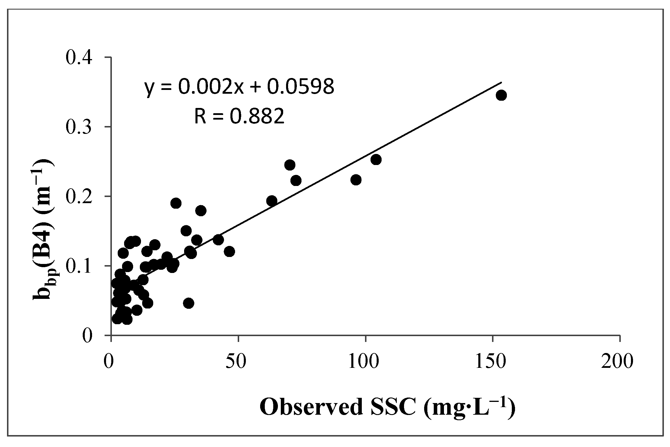
The critical aspect in the semi-analytical models for SSC retrieval is to determine the relationship between SSC and the IOPs of waters. Recently, more research was carried out to study the relationships between IOPs and AOPs [42,43,44,45,46,47]. Among them, the quasi-analytical algorithm (QAA) for the inversion of IOPs developed by Lee et al. [48] based on the reflectance model of Gordon et al. [49] is one of more mature methods with efficient calculation. In the algorithm, only a few empirical relationships were needed [48]. The reflectance model of Gordon et al. [49] used open sea waters and was validated for inland turbid waters by Dekker et al. [50]. It has been used intensively to retrieve SPM in estuarine, coastal and deep waters [28]. The QAA has been used to invert the IOPs of waters off the Chinese coast, e.g., in the Yellow Sea by Hu et al. [51], and in the South Sea coastal area of Fujian by Wang et al. [52]. Nevertheless, further studies are needed to evaluate whether the QAA is generally applicable, especially in coastal regions such as the Gulf of Bohai, China, where large-scale constructions along the coast created varying ocean ecological environments.

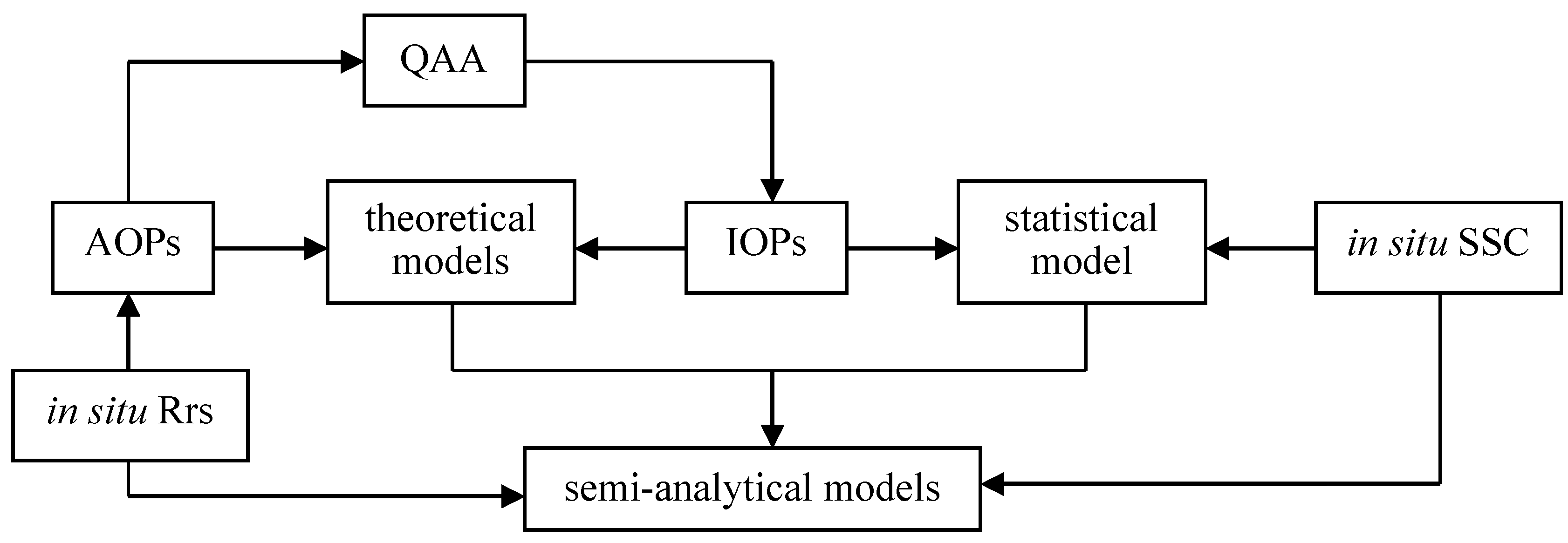
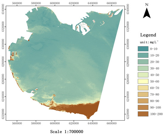
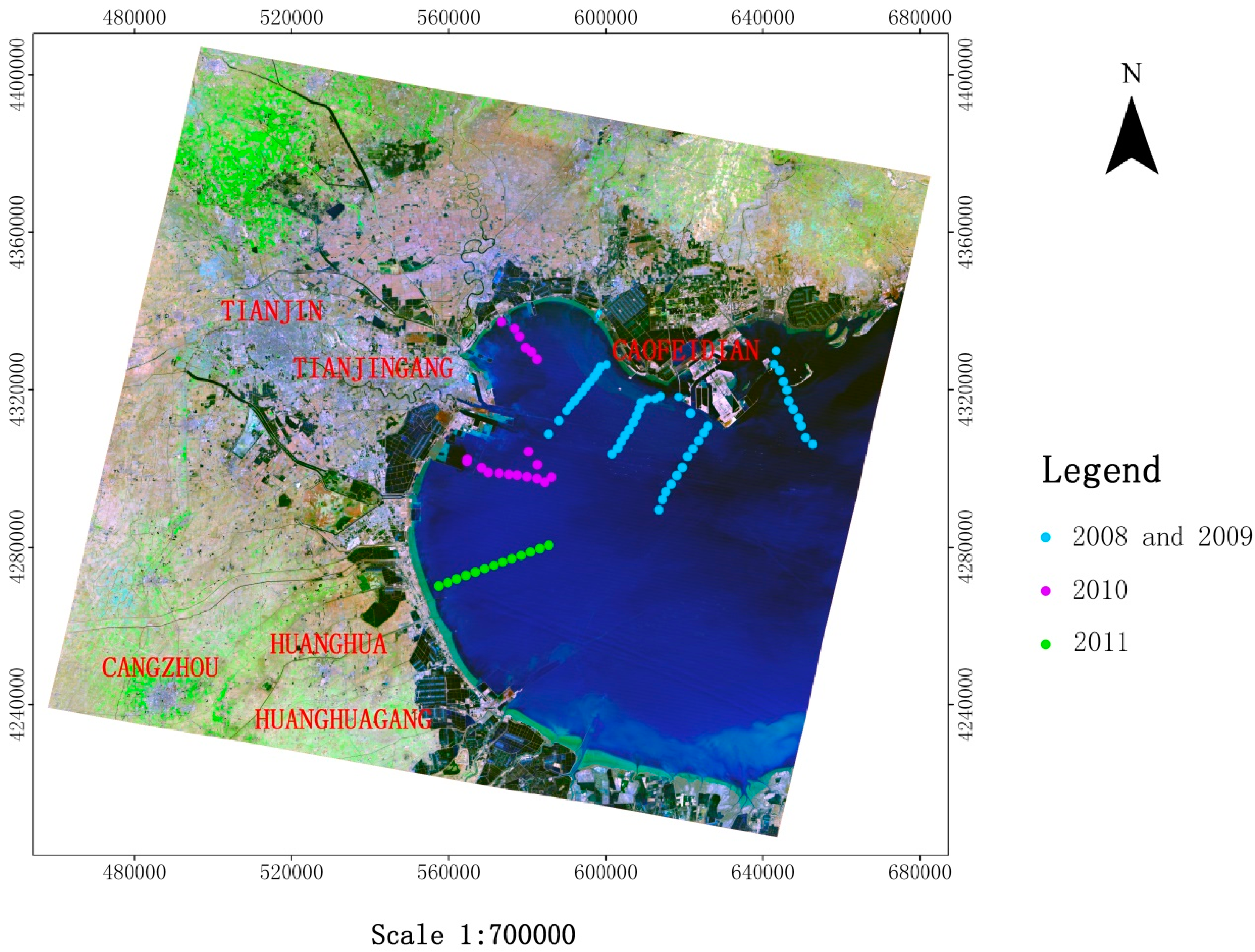
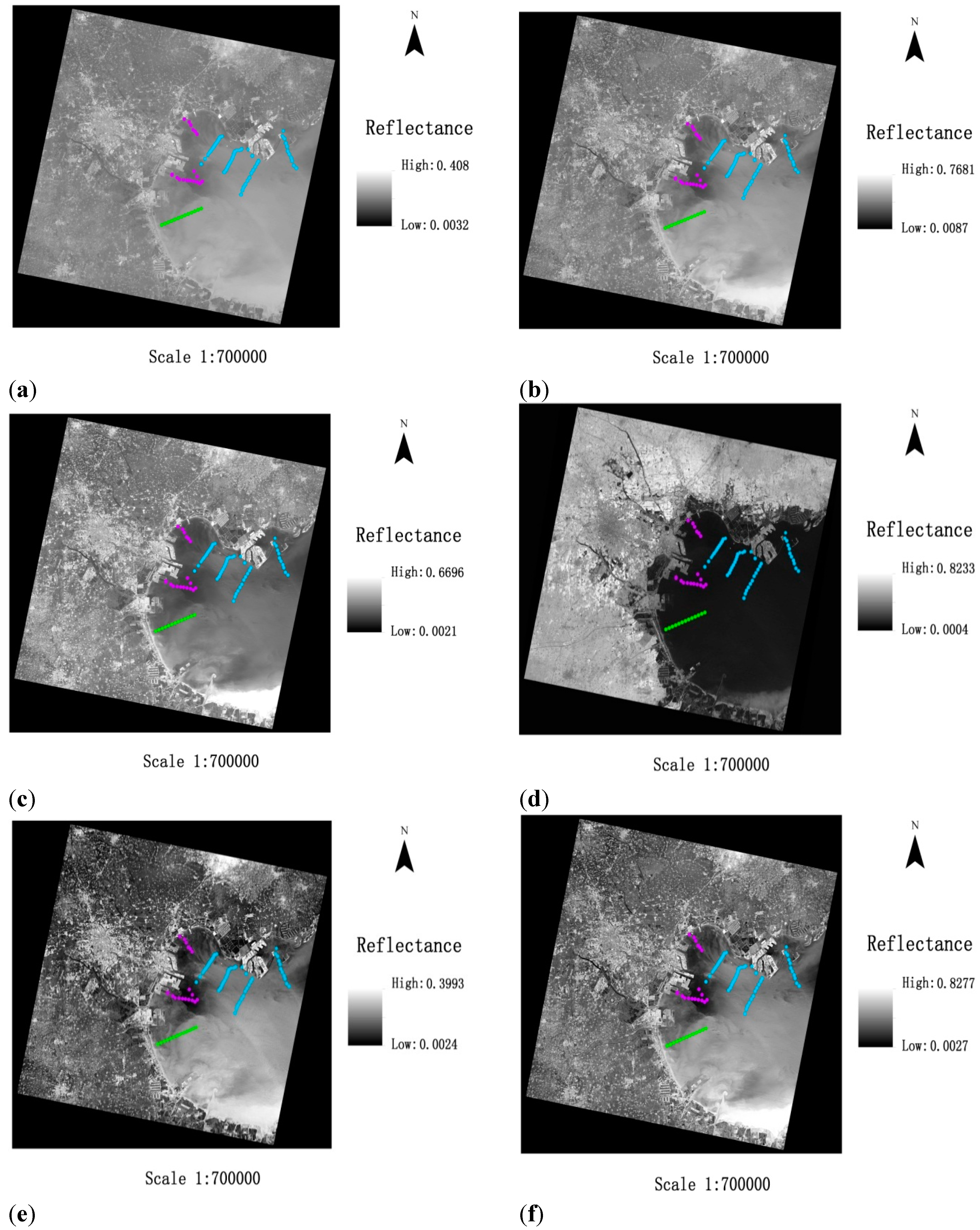
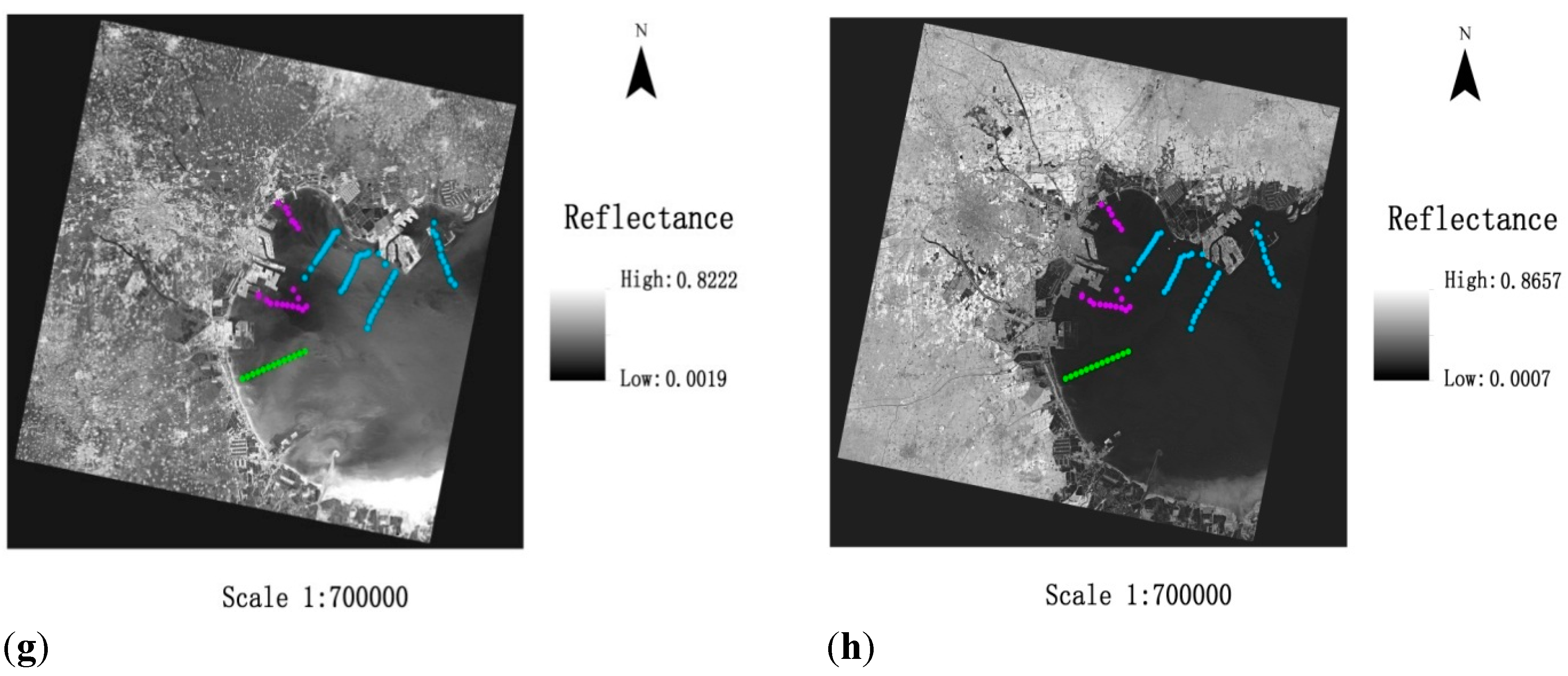
The main objective of this study is to develop a semi-analytical model of remote sensing inversion of SSC for the Gulf of Bohai based on QAA. The algorithm was derived using the information gathered through field observations and from the spectral characteristics of waters in the study area. The semi-analytical model was compared to previous statistical models derived for the Gulf of Bohai, demonstrating its comparatively higher precision and universality. Using the model and TM data, SSC levels of the entire study region were estimated. These estimates can serve as the baseline for a future monitoring of the ocean environment in the Gulf of Bohai in a timely manner.

2. Materials and Methods

2.1. Study Area

The Gulf of Bohai is west of Bohai Sea and is adjacent to the shore of Hebei, Tianjin, and Shandong. It connects Bohai Sea to the Yellow River Estuary. Three large ports are found along the coast of the bay: Tianjin Port, Huanghua Port and Caofeidian Port. The gulf is a sea portal of Beijing-Tianjin and a hub of maritime transport in northern China.

In the Gulf of Bohai, suspended sediment mainly comes from the western end of the region where the southern end is part of the Huanghe (Yellow River) delta region. Sediment deposited at the western end of the bay is transported to the east by tidal waves. Comparing with the Yangtze River estuary and Yellow River estuary [26,53], the study area has in general low SSC, with an average level of 30 mg·L⁻¹.

2.2. Data

The data supporting this study came from two main sources: Space-borne remote sensing data covering the entire study area and its adjacent regions, and a set of in situ data collected from a vessel, including spectral reflectance data measured by a spectrometer and water quality data gathered simultaneously from the field. A total of 107 water samples were collected along 11 transects during the period of 2008 to 2011 (Figure 1). The remote sensing data are one scene of Landsat5 TM images of Bohai Gulf area for 21 September 2011.

2.2.1. In Situ Spectral Reflectance Data and SSC Data

The vessel traversed the region in August 2008, June 2009, August 2010 and September 2011 to collect field data. Among the 11 transects, 4 transects were sampled twice: 2008 and 2009. The distribution of field observations is shown in Figure 1. At each location, radiometric measurements were performed using a double channel spectrometer manufactured by Analytical Spectra Devices (ASD) of the United States. The spectral range covers the spectrum of 350 nm–2500 nm. Spectra measurement of surface waters was taken using the above-water method [54]. The observation geometry is adopted from the International Waters SIMBIOS plans and recommended by Wang et al. (2004) [54], with Φ = 135°, θ = 40° and no shadow effect. Observations were completed under the conditions of wind speed less than 5 m·s⁻¹, cloud coverage less than 10%–20%, and wave height less than 2 m. Survey time was from 9:30 am to 2:30 pm. For each observation, 10 to 20 survey curves were recorded. Based upon the spectral data gathered, spectral curves were derived by the average values. The observed remote sensing reflectance (R_rs) was calculated as:

$$(R_{rs})=\frac{\left(S_{sw}-r\times S_{sky}\right)\times {\rho }_p}{\pi \times S_p}$$

(1)

where, S_sw, S_sky, and S_p are the digital numbers (DNs) when the ASD spectrometer pointed toward the surface waters, the sky and the Lambertian Spectralon plate, respectively; ρ_p is the reflectance of the Lambertian Spectralon plate reported by the system calibration file; r is the reflectance at the interface of water and air, and it is within the range of 0.021 to 0.028. For calm water, r = 0.021. If the wind speed is about 5 m·s⁻¹, r = 0.025. If the wind speed is close to 10 m·s⁻¹, r = 0.028 [55,56].

Figure 1. Sample locations of 11 transects in the Gulf of Bohai from 2008 to 2011. Among the 11 transects, 4 transects in 2008 and 2009 were at the same locations. At each station, radiometric measurements were performed using a double channel spectrometer (ASD). Water samples were also gathered simultaneously.

Figure 1. Sample locations of 11 transects in the Gulf of Bohai from 2008 to 2011. Among the 11 transects, 4 transects in 2008 and 2009 were at the same locations. At each station, radiometric measurements were performed using a double channel spectrometer (ASD). Water samples were also gathered simultaneously.

(R_rs(λ)) was used to derive the equivalent R_rs of Landsat bands via the Landsat spectral response function [57]. The specific formula is:

$$R_{rs}\left({\lambda }_i\right)= {{\displaystyle \int }}_{{\lambda }_s}^{{\lambda }_e}(R_{rs}(\lambda ))F_i(\lambda )d\lambda /{{\displaystyle \int }}_{{\lambda }_s}^{{\lambda }_e}{F}_i(\lambda )d\lambda$$

(2)

where, R_rs(λ_i) is the equivalent R_rs at the central wavelength of Landsat TM band i; F_i(λ) is the spectral response function at band i; and λ_s and λ_e are the start and end wavelengths of band i, respectively.

Table 1. The statistics of the measurements of the study area, including two groups of in situ SSC dataset of 90 locations: One group is the dataset of 70 samples to establish the retrieval model (training data); another group is the dataset of 20 samples to validate the model (testing data); particle size dataset and chlorophyll-a concentration data.

Item	Min	Max	Mean	Samples Number
training data of SSC (mg∙L−1)	2.1	208.7 *	22.5	70
testing data of SSC (mg∙L−1)	6.6	92.2	22.3	20
Particle size (µm)	2.98	72.80	18.56	90
Chlorophyll-a concentration (µg∙L−1)	0.11	1.66	0.57	20

* There is only one sample that SSC is higher than 200 mg∙L⁻¹_.

Table 1. The statistics of the measurements of the study area, including two groups of in situ SSC dataset of 90 locations: One group is the dataset of 70 samples to establish the retrieval model (training data); another group is the dataset of 20 samples to validate the model (testing data); particle size dataset and chlorophyll-a concentration data.

Item	Min	Max	Mean	Samples Number
training data of SSC (mg∙L−1)	2.1	208.7 *	22.5	70
testing data of SSC (mg∙L−1)	6.6	92.2	22.3	20
Particle size (µm)	2.98	72.80	18.56	90
Chlorophyll-a concentration (µg∙L−1)	0.11	1.66	0.57	20

* There is only one sample that SSC is higher than 200 mg∙L⁻¹_.

At each station, water samples were also gathered simultaneously at 0.5 m, 5 m and 10 m below the water surface using special water bottle made of plexiglass. The water bottle was manufactured by Beijing Purity Instrument Company and could sink under water surface up to 30 m for collecting water samples at different depth. Suspended sediment and particle size measurements were obtained from the 107 samples, where SSC levels were determined gravimetrically. Each sample was filtered with a 0.45 μm membrane in a pre-weighted vacuum filter. After drying in a baking oven, the sample was weighed. The particle sizes were measured using the LS-POP (V1) Laser Particle Size Analyzer manufactured by OMEC Company. Chlorophyll-a concentrations were determined for 20 samples, by fluorometry [14,58,59]. Among data gathered from the original 107 sampled locations, data from 90 locations were retained for subsequent analyses since the rest of measurements failed the quality control protocol due to ship waggling, foam in the waters and SSC measurement error. The in situ SSC dataset of 90 locations was divided into two groups: One group is the dataset of 70 samples to establish the retrieval model (training data); another group is the dataset of 20 samples to validate the model (testing data). Along the 11 transects, SSC ranged from 2.1 to 208.7 mg·L⁻¹ (the mean was 20.3 mg·L⁻¹). Particle size measured by the instrument was in the range of 2.98 μm to 72.8 μm (66.27% was between 2 μm and 20 μm, 24.10% was between 20 μm and 50 μm , and 9.63% was larger than 50 μm). According to the observed values, the larger the particle size, the lower were the surface SSC levels and deeper water has larger particle size. Chlorophyll-a concentration spanned from 0.11 to 1.66 µg·L⁻¹ with an average value of 0.57 µg·L⁻¹. The statistics of the measurements are shown in Table 1.

2.2.2. Remote Sensing Data

A scene of Landsat5 TM image (LT51220332011264IKR00) for 21 September 2011 was acquired and processed with atmospheric correction, geometric correction and waters pixels extraction.

(1) Atmospheric correction

For each Landsat5 TM band, the DN values were firstly converted into radiance according to Equation (3) [60]:

$$L_i=GAI{N}_i\times D{N}_i+BIA{S}_i$$

(3)

where, L_i is the at-sensor radiance of TM band i; DN_i is the pixel brightness value; GAIN_i and BIAS_i are the gain coefficient and bias value for the corresponding band i, respectively.

The atmospheric correction for the Landsat data was completed using Fast Line-of-sight Atmospheric Analysis of Spectra Hypercubes (FLAASH), an atmospheric correction module in ENVI^® software [61]. It is based on the non-uniform Lambert surface model within the scope of the solar spectrum (not including thermal radiation) [62]. It can be expressed as:

$$L=\left(\frac{A\rho }{1-{\rho }_{e}s}\right)+\left(\frac{B{\rho }_e}{1-{\rho }_{e}s}\right)+L_{\alpha }$$

(4)

where, L is the radiance received by the sensor; ρ is the reflectance of a pixel; ρ_e is the average reflectance around that pixel; S is the downward hemisphere albedo of the atmosphere; L_α is the atmospheric path radiance including the aerosols and Rayleigh radiances; A and B are the coefficients depending on the atmospheric transmittance and geometric conditions. The difference between ρ and ρ_e is resulted from the neighboring pixels effects caused by atmospheric scattering. The neighboring pixels effects can be corrected using atmospheric point-spread function implemented in the FLAASH module. ρ_e was estimated by:

$${\rho }_e\approx \frac{L_e-L_{\alpha }}{\left[\left(A+B\right)+\left(L_e-L_{\alpha }\right)\times s\right]}$$

(5)

where, L_e is the average radiance of one determined pixel and its surrounding area.

FLAASH directly derives the radiative transfer parameters, which are needed in the atmospheric correction, from the embedded radiative transfer code of MODTRAN4. The surface reflectance is retrieved from the remote sensing image using the standard atmospheric model of MODTRAN4, after selecting the aerosol type. Additional remote sensing inputs are required by the FLAASH model including the location of the area, ground elevation, satellite altitude, flight date, etc. In addition, selections of aerosol model types have a significant influence on the accuracy of atmospheric correction. In this article, mid-latitude summer and maritime types were selected as the parameters of aerosol model type based on the actual situations. Landsat reflectance levels in band 1 to 4 before and after atmospheric correction were shown as Figure 2a–d and e–h, respectively. After atmospheric correction, water reflectance R_w can be obtained.

The remote sensing reflectance spectra, R_rs given at the 4 Landsat central wavelengths (485 nm, 560 nm, 660 nm, 830 nm) for the stations before and after atmospheric correction are shown in Figure 3. The results show that R_rs values of all bands are obviously smaller after atmospheric correction. The variation of R_rs corresponding to the blue band is the most significant, due to the removal of Rayleigh reflectance which is higher in this spectral range. The in situ reflectance and reflectance of Landsat TM band 4 after atmospheric correction (band 4 is the most sensitive band for SSC retrieval) matched well and the correlation coefficient was 0.937.

(2) Geometric correction and water pixels extraction

The image was further geometrically corrected using second-order polynomials. A topographic map of the study area at a scale of 1:50,000 with 35 ground control points was used for the correction. The root-mean-square error (RMSE) for positional accuracy was less than 30 m (1 pixel). A nearest-neighbor re-sampling scheme was used to preserve the DN_s in the original image. A boundary file for the study area was created in GIS (ArcGIS). Using the boundary file, the processed TM image for the study area was identified. To separate water from land pixels, a mask was created using the Normalized Difference Water Index (NDWI) [63].

Figure 2. Landsat reflectance at bands 1 to 4 before (a–d) and after (e–h) the atmospheric correction. The atmospheric correction was completed using Fast Line-of-sight Atmospheric Analysis of Spectra Hypercubes (FLAASH), an atmospheric correction module in ENVI^®.

Figure 2. Landsat reflectance at bands 1 to 4 before (a–d) and after (e–h) the atmospheric correction. The atmospheric correction was completed using Fast Line-of-sight Atmospheric Analysis of Spectra Hypercubes (FLAASH), an atmospheric correction module in ENVI^®.

Figure 3. The graphs of the remote sensing reflectance spectra for the stations before (a) and after (b) atmospheric correction from band 1 to band 4.

Figure 3. The graphs of the remote sensing reflectance spectra for the stations before (a) and after (b) atmospheric correction from band 1 to band 4.

2.3. IOPs Retrieval of the Waters Based on QAA

QAA was originally proposed to retrieve the absorption coefficient $\text{a}(\text{λ})$ and the backscattering coefficient ${\text{b}}_{\text{b}}(\text{λ})$ of waters by Lee et al. [48] based on the model proposed by Gordon et al. [49] that connected the remote sensing reflectance levels with IOPs. According to Gordon et al. 1988 [49]:

$$r_{rs}(\text{λ})=g_0\frac{b_b\left(\lambda \right)}{a\left(\lambda \right)+b_b\left(\lambda \right)}+g_1{\left(\frac{b_b\left(\lambda \right)}{a\left(\lambda \right)+b_b\left(\lambda \right)}\right)}^2$$

(6)

where, $r_{rs}$ represents the remote sensing reflectance just beneath the water surface; $g_0$ and $g_1$ are constants (calculated by Gordon et al. [49] using radiative transfer simulations). In this article, we selected the averaged $g_{0 }$ and $g_1$ values based upon Gordon et al. [49] and Lee et al. [48], i.e., $g_0=0.0895$, $g_1=0.1247 ,$ with a consideration of applying QAA to both coastal and open-ocean waters.

The value of $r_{rs}(\text{λ})$ can be estimated from R_rs, following the model by Lee et al. [48].

$$r_{rs}(\text{λ})=R_{rs}(\text{λ})/(0.52+1.7R_{rs}(\text{λ}))$$

(7)

The total absorption coefficient is generally expressed as the sum of water constituent absorption coefficients

$$a(\text{λ})=a_w(\text{λ})+a_p(\text{λ})+a_g(\text{λ})$$

(8)

where, $a_w$ and $a_p$ stand for the absorption coefficients of pure water and phytoplankton pigments, respectively; and $a_g$ denotes the absorption that is due to the gelbstoff and detritus. The total backscattering coefficient can be expressed as the following:

$$b_b(\text{λ})=b_{bp}(\text{λ})+b_{bw}(\text{λ})$$

(9)

where, $b_{bp}$ and $b_{bw}$ represent the backscattering coefficients of particulates and pure sea waters separately.

In respect to each wavelength, the total absorption coefficient can be expressed as

$$a\left(\lambda \right)=a_w\left(\lambda \right)+\Delta a\left(\lambda \right)$$

(10)

where, $\Delta a\left(\lambda \right)$ stands for the contribution of dissolved and suspended constituents. Lee et al. [35] noted that the value of$\Delta a\left(\lambda \right)$ was quite small at longer wavelengths (>550 nm) with $a\left(\lambda \right)$ mainly determined by the value of $a_w\left(\lambda \right)$, especially in oligotrophic and mesotrophic waters. These facts suggest that, if a reference wavelength ${\lambda }_0$ is found where ${\text{r}}_{\text{rs}}\left({\text{λ}}_0\right)$ from elastic scattering can be accurately measured, then a$\left({\text{λ}}_0\right)$ can be well estimated.

QAA selected 555 nm and 640 nm as the reference wavelength of the Case I and Case II waters, respectively. Considering the waters in this study area is Case II, 640 nm as the reference wavelength (λ₀), subsequently, the absorption coefficient and the backscattering coefficient of wavelength (λ₀) can be estimated by Lee et al. [48].

Then, u(λ) stands for IOPs of waters can be expressed as:

$$u\left(\lambda \right)=\frac{b_b\left(\lambda \right)}{a\left(\lambda \right)+b_b\left(\lambda \right)}$$

(11)

According to Gordon et al. [49], u(λ) can be calculated as follows:

$$u\left(\lambda \right)=\frac{-g_0+{\left[{\left(g_0\right)}^2+4g_1{r}_{rs}\left(\lambda \right)\right]}^{1/2}}{2g_1}$$

(12)

Then $b_{bp}\left(\lambda \right)$ can be expressed as:

$$b_{bp}\left(\lambda \right)=b_{bp}\left({\lambda }_0\right){\left(\frac{{\lambda }_0}{\lambda }\right)}^Y$$

(13)

where, the spectral slope Y is known or can be estimated from remote sensing measurements at any wavelength.

Finally, we can determine the value of $\text{a}\left(\text{λ}\right)$ with a combination of calculated $u\left(\lambda \right)$ and $b_b\left(\lambda \right)$ by Equation (14).

$$a\left(\lambda \right)=\frac{\left(1- u\left(\lambda \right) \right)b_b\left(\lambda \right)}{ u\left(\lambda \right)}$$

(14)

2.4. Developing the Semi-Analytical Model for SSC Retrieval

2.4.1. The Process of Developing the Semi-Analytical Model

IOPs are intermediary parameters in the process of SSC retrieval using the semi-analytical model. The procedure of developing the semi-analytical model in this study is as follows: (i) the in situ reflectance measurements of waters (AOPs) are used in the QAA to obtain the IOPs, then a theoretical model between the AOPs and IOPs based on the radiative transfer theory can be formulated; (ii) analyze the correlation between IOPs and SSC, select the sensitive band or a combination of bands to develop a statistical model between IOPs and SSC; (iii) combine the above two models to construct the semi-analytical model between AOPs and SSC. The process of constructing the semi-analytical model is shown in Figure 4. The entire calculation process was completed using Microsoft Excel 2010^® and IBM SPSS 18.0^®.

Figure 4. The flow diagram of developing the semi-analytical model. The procedure mainly includes three parts: Build a theoretical model between the apparent optical properties (AOPs) and inherent optical properties (IOPs) based on the quasi-analytical algorithm (QAA), select the sensitive band or a bands combination to develop a statistical model between IOPs and suspended sediment concentration (SSC) and combine the above two models to construct the semi-analytical model between AOPs and SSC.

Figure 4. The flow diagram of developing the semi-analytical model. The procedure mainly includes three parts: Build a theoretical model between the apparent optical properties (AOPs) and inherent optical properties (IOPs) based on the quasi-analytical algorithm (QAA), select the sensitive band or a bands combination to develop a statistical model between IOPs and suspended sediment concentration (SSC) and combine the above two models to construct the semi-analytical model between AOPs and SSC.

2.4.2. Developing the Semi-Analytical Model for SSC Retrieval

The ratio u(λ) = b_b(λ)/(a(λ) + b_b(λ)) can be calculated through the QAA algorithm (Equation (11)). The u(λ) and SSC of 70 samples were analyzed of their correlation. As shown in Table 2, u(B4) is the most sensitive factor (R = 0.914). This is consistent with the studies by Onderka et al. [14], Chen et al. [64] and Li et al. [65]. In addition, u(B4/B1) has a better performance.

Table 2. The correlation coefficients between SSC measurements and the associated u = b_b/(a + b_b) retrieved from R_rs measurements using QAA, given various Landsat5 TM bands and band ratios.

u	u(B2)	u(B3)	u(B4)	u(B4/B3)	u(B4/B2)	u(B4/B1)	u(B3/B2)	u(B3/B1)
R *	0.563	0.764	0.914	0.501	0.813	0.851	0.783	0.789

* R: The correlation coefficient between SSC and u(B_i). B_i stands for the central wavelength of band i for TM data.

Table 2. The correlation coefficients between SSC measurements and the associated u = b_b/(a + b_b) retrieved from R_rs measurements using QAA, given various Landsat5 TM bands and band ratios.

u	u(B2)	u(B3)	u(B4)	u(B4/B3)	u(B4/B2)	u(B4/B1)	u(B3/B2)	u(B3/B1)
R *	0.563	0.764	0.914	0.501	0.813	0.851	0.783	0.789

* R: The correlation coefficient between SSC and u(B_i). B_i stands for the central wavelength of band i for TM data.

Since u(B4) is the most sensitive factor, it was selected to establish a variety of statistical models. Five types of models were developed to evaluate the relationship between u(B4) and SSC levels. The quadratic model has relatively high R² (R² = 0.922). Specifications of the model and regression result are reported in Table 3.

Table 3. The fitting degree for different regression model between the sensitive factor u(B4) and SSC levels.

Model Type	Linear	Logarithmic	Quadratic	Power	Exponential
R2	0.835	0.510	0.922	0.536	0.598

Table 3. The fitting degree for different regression model between the sensitive factor u(B4) and SSC levels.

Model Type	Linear	Logarithmic	Quadratic	Power	Exponential
R2	0.835	0.510	0.922	0.536	0.598

Considering the R² of each model, we selected the quadratic polynomial model (Equation (15)) as the statistical model between u and SSC levels.

$$SSC=8.602-109.742\times u\left(B4\right)+3328.547\times {[u\left(B4\right)]}^2$$

(15)

As the semi-analytical model developed by the IOPs of waters simulates the remote sensing reflectance just beneath the water surface, it is necessary to convert the subsurface irradiance reflectance $\text{R}\left(\text{λ},0^{-}\right)$to the above-surface reflectance ${\text{R}}_{\text{rs}}\left(\text{λ}\right)$ measured in the field. Gordon [66] constructed a polynomial model for the subsurface irradiance reflectance, R(λ,0⁻), as a function of absorption and backscattering coefficients of waters based on Monte Carlo simulation, and it can be expressed as:

$$R\left(\lambda ,0^{-}\right)=f\left({\mu }_0\right)\frac{b_b\left(\lambda \right)}{a\left(\lambda \right)+b_b\left(\lambda \right)}=\frac{E_U\left(\lambda ,0^{-}\right)}{E_D\left(\lambda ,0^{-}\right)}$$

(16)

The value of $f\left({\mu }_0\right)$ depends on the solar zenith angle, cloud cover, sea conditions, and the shape of body scattering function etc., ${\text{E}}_{\text{U}}\left(\text{λ},0^{-}\right)$ and ${\text{E}}_{\text{D}}\left(\text{λ},0^{-}\right)$ are upwelling and downwelling irradiance just beneath the water surface, respectively.

Previous studies have reported on the value of $f\left({\mu }_0\right)$. Kirk [67] reported that the value of $f\left({\mu }_0\right)$ should have a range from 0.33 to 0.38 in his study. In this article, 0.34 was finally adopted according to relevant literatures [68,69], and $E_U\left(\lambda ,0^{-}\right)$ and $E_D\left(\lambda ,0^{-}\right)$ are defined in Equations (17) and (18), respectively.

$$E_U\left(\lambda ,0^{-}\right)=Q\times L_U\left(\lambda ,0^{-}\right)$$

(17)

$$E_D\left(\lambda ,0^{-}\right)=\left(1-{{\rm P}}_{aw}\right)\times E_D\left(\lambda ,0^{+}\right)$$

(18)

where, Q is the parameter of light field distribution in the waters, and it is influenced by water content, solar altitude and observation angle. Its value can be calculated from the sun angle (Gons, 1999 [70]) and usually ranges between 1.7 and 7.0; ${{\rm P}}_{aw}$ is the irradiance reflectance at the interface of air and water, and it is generally between 0.04 and 0.06. In addition, the upward radiance just beneath the water surface $L_U\left(\lambda ,0^{-}\right)$ can be expressed as:

$$L_U\left(\lambda ,0^{-}\right)=\frac{n^2}{t}\times L_w\left(\lambda ,0^{+}\right)$$

(19)

where, t represents the Fresnel transmission coefficient in the air-water surface, and n stands for refractive index of water. Moreover, according to the definition of the above-surface remote sensing reflectance:

$$R_{rs}\left(\lambda \right)=\frac{L_w\left(\lambda ,0^{+}\right)}{E_D\left(\lambda ,0^{+}\right)}$$

(20)

where, $R_{rs}\left(\lambda \right)$ is the remote sensing reflectance, $L_w\left(\lambda ,0^{+}\right)$ is the water-leaving radiance of the incident light and $E_D\left(\lambda ,0^{+}\right)$ stands for the downward irradiance of the incident light. Therefore, according to the above equations Equations (16)–(20):

$$R\left(\lambda ,0^{-}\right)=R_{rs}\left(\lambda \right)\times \frac{Q{n}^2}{t\left(1-{{\rm P}}_{aw}\right)}$$

(21)

According to relevant studies [71,72] and our test, the values of Q, n, t and ${{\rm P}}_{aw}$ are finally determined to be 2.9, 1.34, 0.98 and 0.05, respectively. The relationship between the above-surface remote sensing reflectance and subsurface reflectance is expressed in Equaiton (22):

$$R\left(\lambda ,0^{-}\right)=5.59\times R_{rs}\left(\lambda \right)$$

(22)

Combining Equations (11) and (16) with Equation (22), the relational model of AOPs and IOPs is:

$$u\left(B4\right)=16.45\times R_{rs}\left(B4\right)$$

(23)

Finally, the semi-analytical model for the SSC retrieval can be established by combining Equations (15) and (23):

$$SSC=8.602-1805.26\times R_{rs}B4+900713.14\times {[R_{rs}\left(B4\right)]}^2$$

(24)

2.5. Statistical Criteria for Model Performance

To evaluate the models performance, we applied three statistical indices, i.e., the absolute residuals (AR), the relative error (RE) and the root-mean-squared error (RMSE). These statistical indices are described by

$$AR=\left|SS{C}_{mod,i}-SS{C}_{obs,i}\right|$$

(25)

$$RE= \left|\frac{SS{C}_{mod,i}-SS{C}_{obs,i}}{SS{C}_{obs,i}}\right|\times 100\%$$

(26)

$$RMSE=\sqrt{\frac{{{\displaystyle \sum }}_1^n{\left(SS{C}_{mod,i}-SS{C}_{obs,i}\right)}^2}{n}}$$

(27)

where, SSC_mod,i is the estimated SSC using the retrieval model corresponding to sample i, SSC_obs,i is the observed SSC of sample i, and n is the number of samples.

3. Results and Discussion

3.1. Spectral Characteristics of Waters

The in situ reflectance spectra collected from each station were analyzed and averaged after unreliable data were removed from the dataset. The reflectance spectrum at each station was then calculated using Equation (1). Figure 5 shows the reflectance spectral curves developed for selected samples covering a range of SSC levels. In the graph, each curve at a given SSC level shows the relationship between the spectral ranges and reflectance levels. While the spectrometer captures spectra within a wider range, reflectance of sea surface waters beyond 900 nm is rather low due to the effect of water absorption. Therefore, we focus on the spectral bands within the range of 400 to 900 nm.

In general, the higher the SSC levels, the higher are the reflectivity levels over the band region of 400–900 nm. Given an SSC level, reflectivity is higher around 570 nm, 670 nm and 800 nm. Two reflection peaks are apparent with the larger one in the region between 500 to 700 nm and a smaller one in 780 to 830 nm. Responses to SSC increase between 400 to 580 nm, but decline from 580 nm to approximately the 730–750 nm range. Obviously, sensitivities across band widths increase with SSC levels. This characteristic is important for the retrieval of SSC from remote sensing data in different waters.

A key to establish quantitative retrieval models of SSC is to select responsive spectral bands. In our study, reflectance data collected from the spectrometer shows two peaks. These peak regions, which indicate the spectra relatively sensitive to SSC levels, were found in band 2–4 (TM2, TM3 and TM4) in the Landsat5 data. In developing the retrieval models, the effectiveness of these individual bands or combinations of some of them will be explored.

Figure 5. Remote sensing reflectance (sr⁻¹) corresponding to different wavelengths (nm) for selected SSC levels. Each curve at a given SSC level shows the relationship between the spectral ranges and reflectance levels.

Figure 5. Remote sensing reflectance (sr⁻¹) corresponding to different wavelengths (nm) for selected SSC levels. Each curve at a given SSC level shows the relationship between the spectral ranges and reflectance levels.

3.2. The Relationship between Inversed b_bp and SSC

The relationship between inversed b_bp and observed SSC was established, as shown in Figure 6. The two factors show a linear relationship (correlation coefficient r = 0.882): The backscattering coefficients increased with SSC. When SSC is below 50 mg·L⁻¹, the deviations of b_bp in the samples are slightly larger than those when SSC is above 50 mg·L⁻¹. As lower sediment concentrations are associated with larger particle sizes in the study area, the result shows that particle size has an influence on b_bp.

Figure 6. The relationship between inversed b_bp using QAA and observed SSC. The two factors show a linear relationship (correlation coefficient r = 0.882).

Figure 6. The relationship between inversed b_bp using QAA and observed SSC. The two factors show a linear relationship (correlation coefficient r = 0.882).

3.3. Model Evaluation

3.3.1. The Accuracy of the Model

In order to evaluate the performance of the retrieval model identified above, we applied this model to predict the SSC levels based upon the reflectance R_rs(B4) derived from in situ measurements of the remaining 20 sampled points. The predicted SSC levels from the model are compared with the values observed in the field. Their differences are residuals. The accuracy of the model is acceptable with a mean relative error and a root-mean-squared error (RMSE) of 12.32% and 4.53 mg·L⁻¹, respectively. Analyzing the accuracy of the model, we found that the absolute residuals are basically within 2Δ (Δ is the mean error) and the relative errors are less than 20%, except for two samples.

3.3.2. Comparing the Performance with Empirical Model

The same observed dataset including the remote sensing reflectance and SSC levels that were used to develop the semi-analytical model, were also used to establish the empirical model. According to the correlation analysis between TM band reflectance and SSC, band 4 is the most sensitive band (R = 0.8596). The quadratic model among various types of band 4 has a relatively high coefficient of determination (R² = 0.844). Therefore, the quadratic model was adopted as the empirical retrieval model. As shown in Equation (28), the model is specified as

$$SSC=5.184+1349.63\times Rrs\left(B4\right)+614561.673\times {[Rrs\left(B4\right)]}^2$$

(28)

The empirical model was used to estimate the SSC levels. The estimated SSC of the 20 validation points were compared with the in situ observations. Meanwhile, the accuracy of the model was calculated. The comparison of relative errors and RMSE between the semi-analytical model and empirical model is summarized in Table 4. Results show that the performance is generally similar for the two type models, but the semi-analytical model has a slight edge over the other.

Table 4. The comparison of the performance between semi-analytical model and empirical model using the testing dataset of 20 validation points.

Model Type	Largest RE (%)	Smallest RE (%)	Mean RE (%)	RMSE (mg L−1)
Semi-analytical	31.20	0.94	12.32	4.53
Empirical	46.24	0.08	17.67	5.59

Table 4. The comparison of the performance between semi-analytical model and empirical model using the testing dataset of 20 validation points.

Model Type	Largest RE (%)	Smallest RE (%)	Mean RE (%)	RMSE (mg L−1)
Semi-analytical	31.20	0.94	12.32	4.53
Empirical	46.24	0.08	17.67	5.59

Figure 7. (a) The comparison of retrieved SSC levels using semi-analytical model and empirical model. (b) The first derivative functions of semi-analytical model and empirical model. (c) The relationship between observed SSC and SSC estimated by the two models.

Figure 7. (a) The comparison of retrieved SSC levels using semi-analytical model and empirical model. (b) The first derivative functions of semi-analytical model and empirical model. (c) The relationship between observed SSC and SSC estimated by the two models.

For further comparison of the two models, we estimated the SSC levels by the semi-analytical model and empirical model within the range of observed R_rs(B4) at an interval of 0.0005 (sr⁻¹). As shown in Figure 7a, the retrieved SSC levels from the two models have the same trend versus the remote sensing reflectance R_rs(B4). The differences between the retrieved SSC levels from the two models are relatively small with the maximum, the minimum and the mean values of 25.00 mg·L⁻¹, 0.06 mg·L⁻¹ and 6.51 mg·L⁻¹, respectively. However, when the reflectance R_rs(B4) increases, the difference becomes larger (when R_rs(B4) > 0.0113 sr⁻¹, equivalently SSC > 100 mg·L⁻¹). These increasing differences may be due to the fact that the SSC levels that were used to develop the models are relative low. The observed SSC values of the 70 sample points, with the exception of two, were less than 100 mg·L⁻¹. The result shows that the semi-analytical model results are consistent with those from the empirical model.

Meanwhile, the first derivatives of the semi-analytical and empirical model functions were derived to analyze the changes of SSC versus the variations of R_rs(B4), and the results are as shown in Figure 7b. Obviously, there is a divergent point (when R_rs(B4) = 0.0053 sr⁻¹ and SSC’ = 7904.54 mg·L⁻¹/sr⁻¹), which corresponds to the mean level of SSC estimated by the models. Above this point, the semi-analytical model is more sensitive to changes in remote sensing reflectance than the empirical model. In addition, the former model is more effective than the latter model for SSC retrieval. Below the divergence point, the result is the opposite.

In addition, as shown in Figure 7c, the estimated SSC levels are high relative to the observed values in the field. The correlation between the observed and estimated values from the semi-analytical model is 0.95 and between the observed and estimated values from the empirical model is 0.94.

The efficiency of the model is different with SSC levels. The statistics of retrieval accuracy (in logarithm space) of the semi-analytical model for different SSC ranges corresponding to 90 samples were shown in Table 5. For SSC > 50 mg·L⁻¹, the performance of the model is better, because the remote sensing reflectance is relatively larger and there is a strong relationship between SSC and R_rs(B4) in TM4 band. R_rs is more sensitive to the variety of SSC level. For SSC < 50 mg·L⁻¹, the performance of this model is slightly worse as compared to its performance with higher SSC levels. This is caused by the fact that R_rs in this SSC range is not too sensitive to SSC levels and the difference between R_rs is small in TM4 band. However, when SSC is below 20 mg·L⁻¹, the performance of the model is improved. The main reason is that the sample points in the study area had generally lower SSC levels (the average value < 30 mg·L⁻¹), and most SSC data that were used to develop the retrieval model were less than 20 mg·L⁻¹ (53 points of 70 modeling points in this range). In addition, when observed SSC levels were less than 10 mg·L⁻¹, the estimated SSC was always higher than 7 mg·L⁻¹ (as shown in Figure 7c). The performance of the model is relatively worse in this SSC range (Table 5). It shows that the retrieval model has a low sensitivity to the lower concentration. Therefore, the performance of the retrieval model is different with SSC levels. The model is more reliable for SSC retrieval when SSC is higher than 10 mg·L⁻¹.

Table 5. The statistics of retrieval accuracy (in logarithm space) of the semi-analytical model for different SSC ranges corresponding to 90 samples in the study area.

The range of SSC (mg∙L−1)	0–10	10–20	20–50	>50
MAR * (in log scale/mg∙L−1)	0.22	0.16	0.35	0.13

* MAR is the mean absolute residuals.

Table 5. The statistics of retrieval accuracy (in logarithm space) of the semi-analytical model for different SSC ranges corresponding to 90 samples in the study area.

The range of SSC (mg∙L−1)	0–10	10–20	20–50	>50
MAR * (in log scale/mg∙L−1)	0.22	0.16	0.35	0.13

* MAR is the mean absolute residuals.

Comparing the accuracy of the proposed model with four empirical statistical models developed for the study area, the Mean Relative Errors (MREs) for different models are reported in Table 6 [65,73,74]. The results show that the semi-analytical model yields the lowest MRE, providing better estimates of SSC than other empirical models. The proposed model is more suitable for SSC retrieval for the Gulf of Bohai where SSC levels are relatively low with an average value below 30 mg·L⁻¹.

Table 6. The summary of comparing the accuracy of the proposed semi-analytical model with previous empirical models in the study area.

No.	Nt/Nm*	Retrieval Models	Mean RE (%)	Model Type	Authors
1	90/70	SSC = 8.602−1805.26 × Rrs(B4) + 900713.14 × [Rrs(B4)]2	12.32	Semi-analytical	Kong, J.L.
2	32/25	ln SPM = 153.85 × Rrs(B3) + 1.11	21.19	Empirical	Li, J.G. [65]
3	45/33	lg(SPM) = −2.1302 − 1.0205 × Rrs(709)/Rrs(443) + 3.8018 × (Rrs(709)/Rrs(560))	28.30	Empirical	Chen, L. [73]
4	34/23	SSC = 53.273 × (Rrs(645)/Rrs(555))2 − 31.05 × (Rrs(645)/Rrs(555)) + 8.357	29.48	Empirical	Cui, J. [74]
5	36/29	SSC = 319.637 × (Rrs(645)/Rrs(555))2 − 379.247 × (Rrs(645)/Rrs(555)) + 120.905	15.96	Empirical	Cui, J. [74]

* N_t is the total samples number; N_m is the samples number for modeling.

Table 6. The summary of comparing the accuracy of the proposed semi-analytical model with previous empirical models in the study area.

No.	Nt/Nm*	Retrieval Models	Mean RE (%)	Model Type	Authors
1	90/70	SSC = 8.602−1805.26 × Rrs(B4) + 900713.14 × [Rrs(B4)]2	12.32	Semi-analytical	Kong, J.L.
2	32/25	ln SPM = 153.85 × Rrs(B3) + 1.11	21.19	Empirical	Li, J.G. [65]
3	45/33	lg(SPM) = −2.1302 − 1.0205 × Rrs(709)/Rrs(443) + 3.8018 × (Rrs(709)/Rrs(560))	28.30	Empirical	Chen, L. [73]
4	34/23	SSC = 53.273 × (Rrs(645)/Rrs(555))2 − 31.05 × (Rrs(645)/Rrs(555)) + 8.357	29.48	Empirical	Cui, J. [74]
5	36/29	SSC = 319.637 × (Rrs(645)/Rrs(555))2 − 379.247 × (Rrs(645)/Rrs(555)) + 120.905	15.96	Empirical	Cui, J. [74]

* N_t is the total samples number; N_m is the samples number for modeling.

3.4. Application of the Model

Using the semi-analytical model (Equation (24)), the SSC levels for the Gulf of Bohai were derived from the atmospherically-corrected TM data (Figure 8). From the inversion of TM-derived R_rs map, SSC levels are generally lower in the study area (the average concentration level is 27 mg·L⁻¹), mainly concentrated in the region with an SSC level less than mg·L⁻¹ and accounted for 86.42% of the total area. The distribution of SSC levels is shown in detailed in Table 7. The distribution of SSC levels exhibits several characteristics: (i) in general, SSC levels in the southern part were higher than those in the northern part of the study area; (ii) SSC levels have a slight fluctuation from the offshore area to the deep sea and show a general decrease. These two characteristics also reveal the sources of sediment in the Gulf of Bohai: (i) as the southern water is the estuary of the Yellow River, it receives a large amount of sediment carried by the Yellow River; (ii) due to the severe impact of intense human activities in the coastal areas, especially in the nearby ports, SSC levels were higher in the coastal areas than those in the deep sea; (iii) re-suspended sediment is one of the sources of sediment in the shallow regions, where SSC is higher in these areas.

Figure 8. The image map of SSC distribution derived from the atmospherically-corrected TM data using the semi-analytical model for the Gulf of Bohai.

Figure 8. The image map of SSC distribution derived from the atmospherically-corrected TM data using the semi-analytical model for the Gulf of Bohai.

Table 7. Statistics of SSC levels derived from the atmospherically-corrected TM data using the semi-analytical model in different ranges.

SSC (mg·L−1)	0–10	10–20	20–30	30–40	40–50	50–100	100–200	>200
Area (km2)	227.12	4927.00	3625.32	458.82	167.82	184.67	137.57	431.07
Percentage (%)	2.24	48.50	35.68	4.52	1.65	1.81	1.35	4.24

Table 7. Statistics of SSC levels derived from the atmospherically-corrected TM data using the semi-analytical model in different ranges.

SSC (mg·L−1)	0–10	10–20	20–30	30–40	40–50	50–100	100–200	>200
Area (km2)	227.12	4927.00	3625.32	458.82	167.82	184.67	137.57	431.07
Percentage (%)	2.24	48.50	35.68	4.52	1.65	1.81	1.35	4.24

4. Conclusions

The Gulf of Bohai area is labeled as the top priority region of the circular economic development zone by the Chinese Government in the last ten years. Large-scale constructions cause significant changes in the ocean’s ecological environment. It is important to monitor the ocean’s ecological environment by quantitative remote sensing in a timely manner.

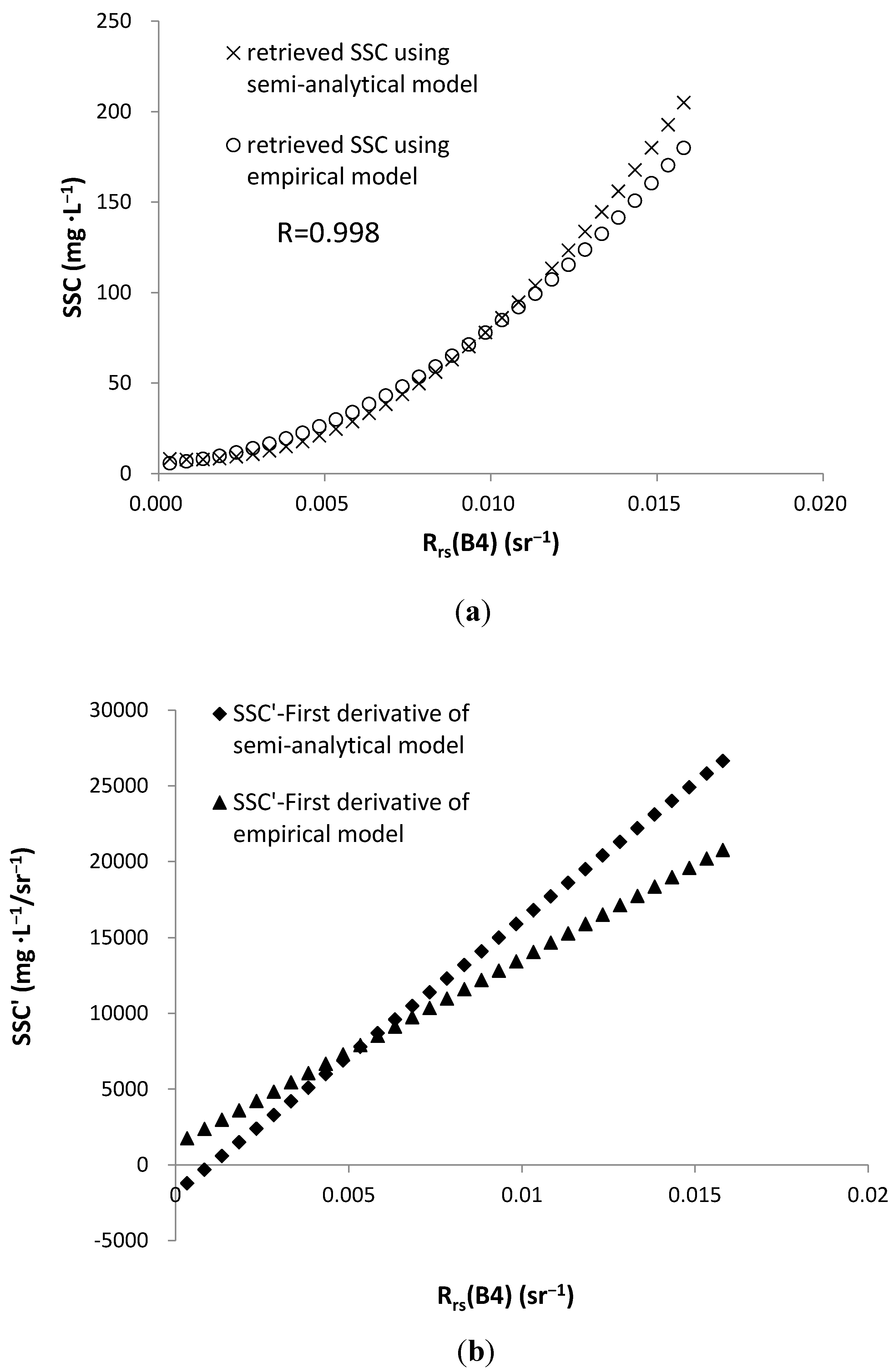
SSC is one of the critical parameters in ocean environmental evaluation. SSC levels in the Gulf of Bohai are relatively low, hence, an effective inversion model should have high sensitivity and stability. Existing models are mostly statistical models, based on the correlation between the apparent optical properties (remote sensing reflectance) and SSC levels. Because remote sensing reflectance is associated with the conditions of observation and the geographical scope of the waters, empirical statistical models are of limited applications. The semi-analytical model developed in this article, based on the QAA algorithm, investigated the relationship between IOPs of waters constitutes and remote sensing reflectance. Because IOPs are related to the inherent nature of waters and do not vary with the conditions of observation, the semi-analytical model showed a higher precision and universality than the empirical models.

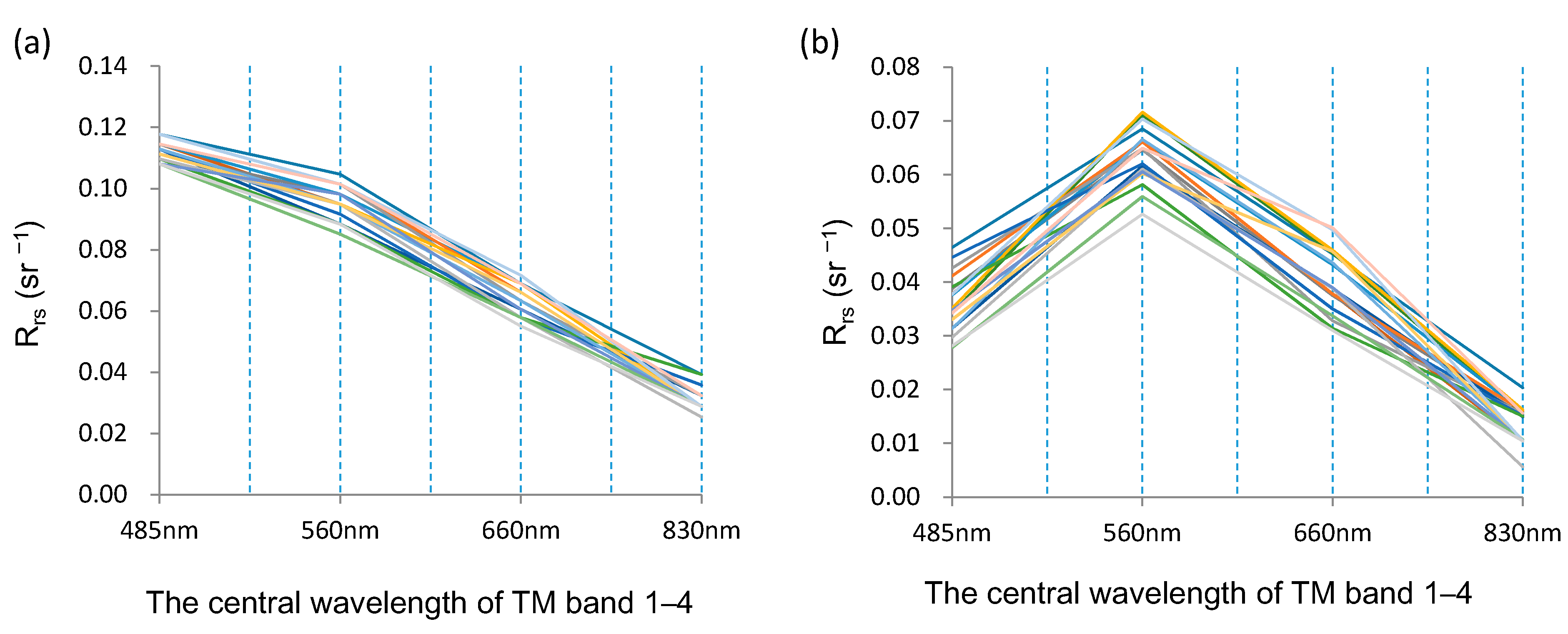
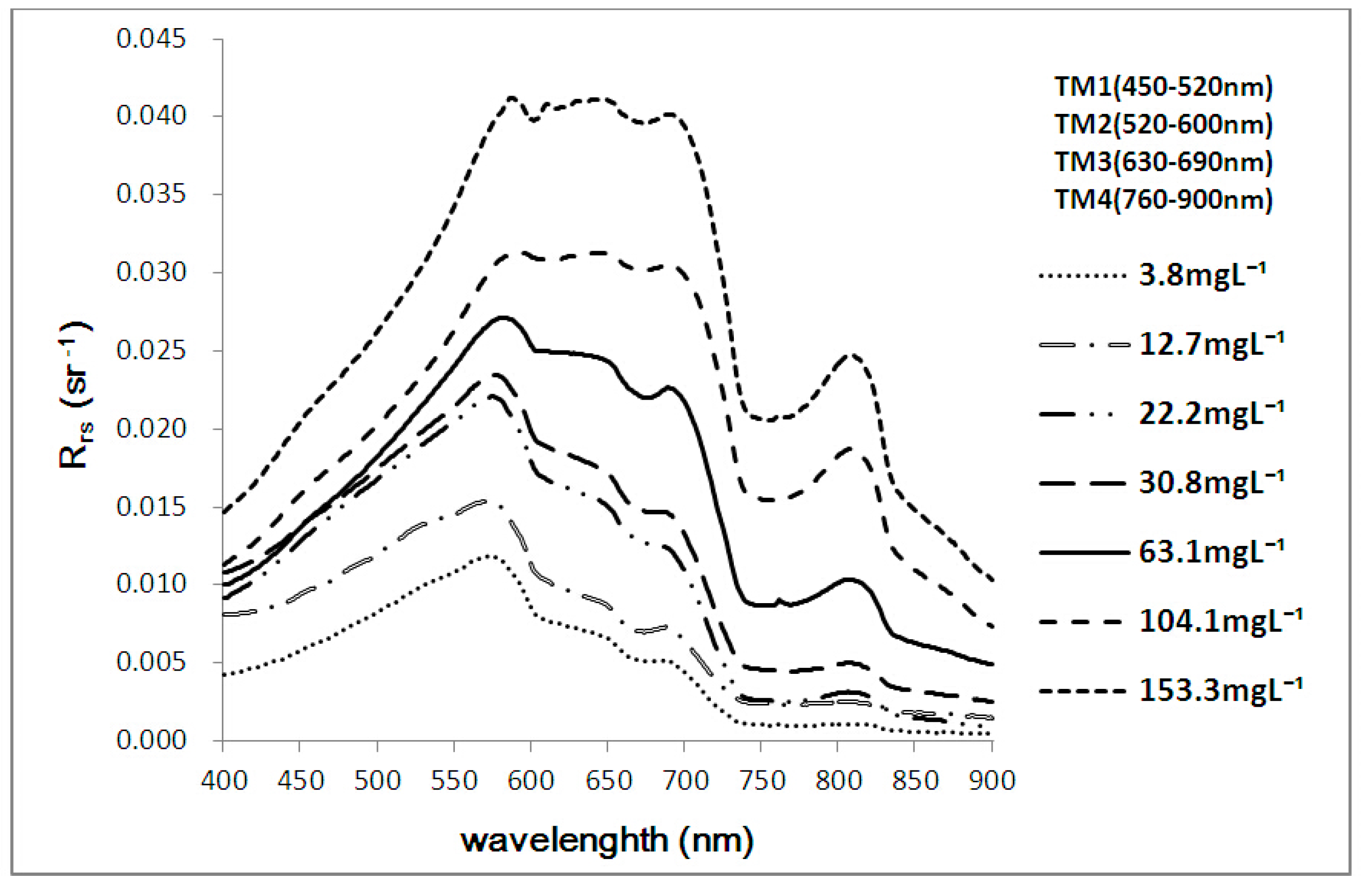
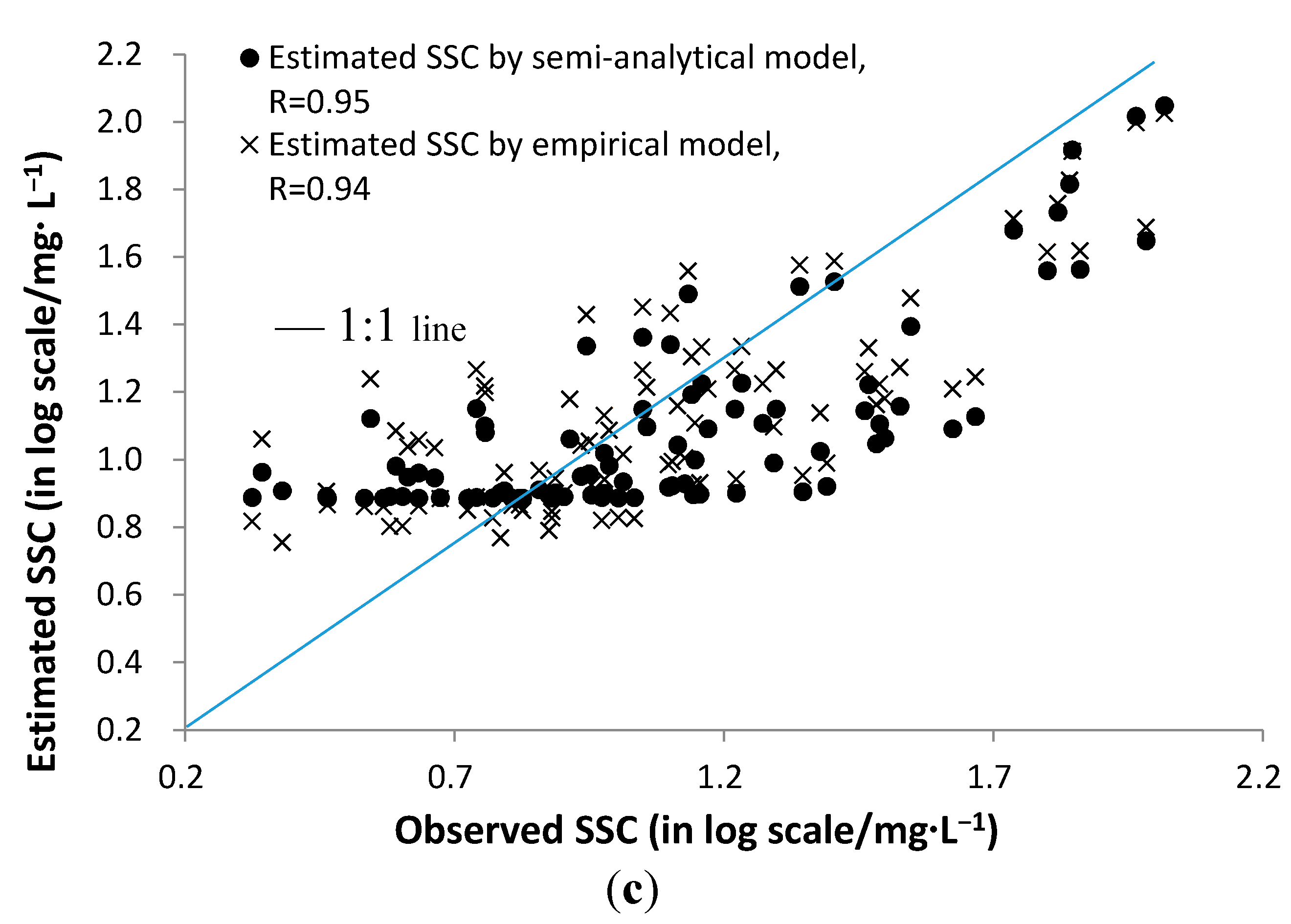
The study results indicated that the most sensitive band to SSC levels in the study area is the NIR band of Landsat5 TM images. This finding is consistent with the studies by Onderka et al. [13], Chen et al. [66] and Li et al. [67]. A quadratic polynomial semi-analytical model is proposed as an SSC retrieval model based on the relationship between the inherent optical properties and apparent optical properties of water using the QAA. According to 20 validation points, the accuracy of the model has an average relative error of 12.32% and the RMSE of 4.53 mg·L⁻¹ while the correlation coefficient between observed and estimated SSC is 0.95. 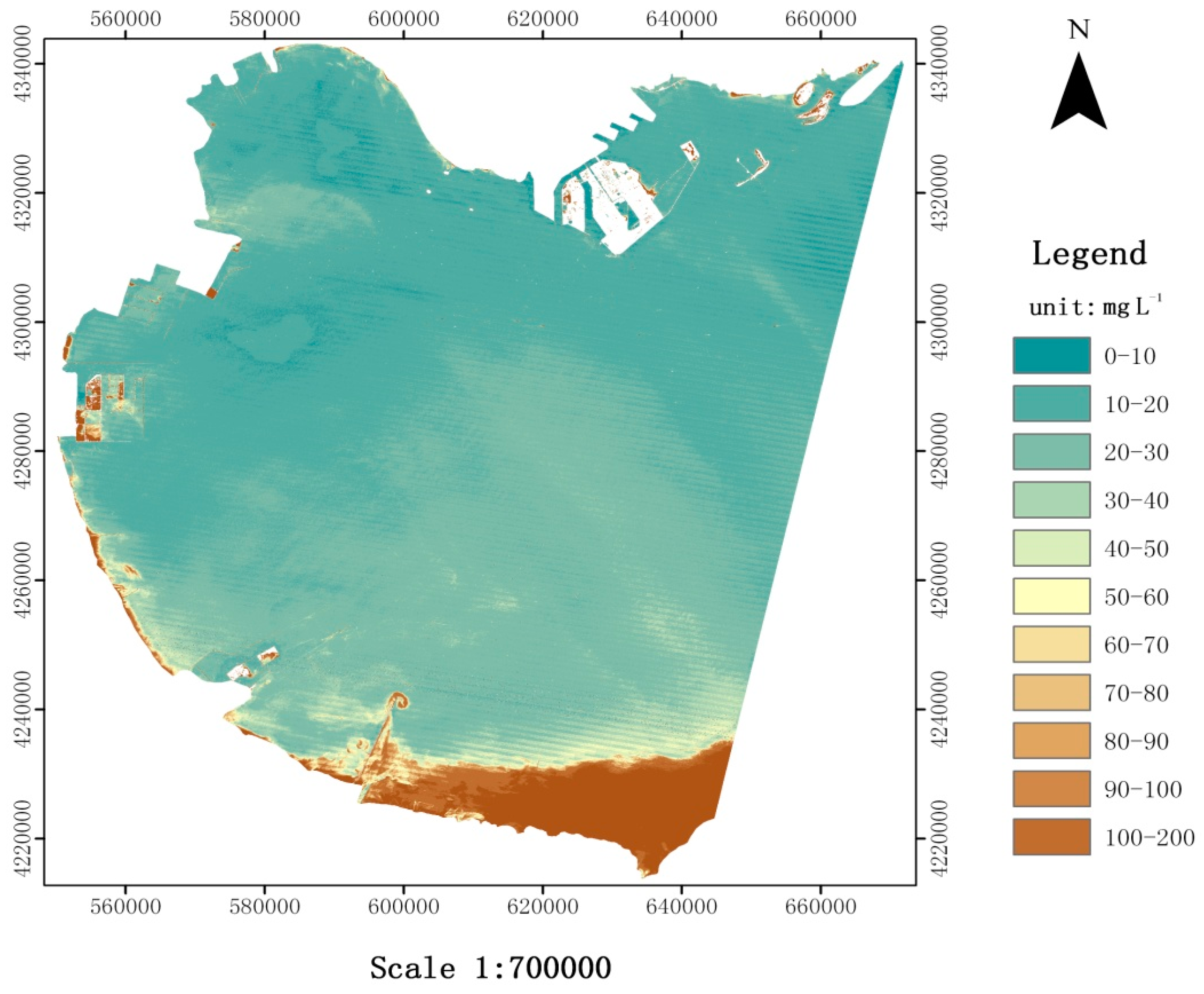Unlike the empirical statistical model that was developed using the same in situ data, the semi-analytical model is more sensitive to the changes of the remote sensing reflectance. Compared with the previous statistical models used in other studies, the semi-analytical model that includes a relationship between reflectance, IOPs and SSC shows a slightly higher precision. Using the retrieval model and TM data, SSC levels of the entire study region were estimated. The distribution characteristics of SSC levels revealed the sources of sediment in the Gulf of Bohai which was carried by the Yellow River to the estuary in the southern part, re-suspended sediment in the shallow regions and due to the human activities effects along the coastal areas, especially in the nearby Huanghua Port. The study results can serve as the baseline for future monitoring of the ocean environment in the region.

References

1. Wang, X.Q.; Chen, C.C. Application of remote sensing to environmental monitoring in coastal waters. Mar. Environ. Sci. 2000, 19, 72–76. (In Chinese) [Google Scholar]
2. Yu, G.L.; Yang, W.; Matsushita, B.K.; Li, R.H.; Oyama, Y.; Fukushima, T. Remote estimation of chlorophyll-a in inland waters by a NIR-Red-based algorithm: Validation in Asian Lakes. Remote Sens. 2014, 6, 3492–3510. [Google Scholar] [CrossRef] [Green Version]
3. EI-Alem, A.; Chokmani, K.; Laurion, I.; EI-Adlouni, S. An adaptive model to monitor chlorophyll-a in inland waters in southern Quebec using downscaled MODIS imagery. Remote Sens. 2014, 6, 6446–6471. [Google Scholar] [CrossRef]
4. Devred, E.; Turpie, K.R.; Moses, W.; Klemas, V.V.; Mosian, T.; Babin, M.; Toro-Farmer, G.; Forget, M.H.; Jo, Y.H. Future retrievals of water column bio-optical properties using the Hyperspectral Infrared Imager (HyspIRI). Remote Sens. 2013, 5, 6812–6837. [Google Scholar] [CrossRef]
5. Buckton, D.; O’Mongain, E.; Danaher, S. The use of neural networks for the estimation of oceanic constituents based on the MERIS instrument. Int. J. Remote Sens. 1999, 20, 1841–1851. [Google Scholar] [CrossRef]
6. Koponen, S.; Attila, J.; Pulliainen, J.; Kallio, K.; Pyhälahti, T.; Lindfors, A.; Rasmus, K; Hallikainen, M. A case study of airborne and satellite remote sensing of a spring bloom event in the Gulf of Finland (Baltic Sea). Cont. Shelf Res. 2007, 27, 228–244. [Google Scholar] [CrossRef]
7. Stumpf, R.P.; Pennock, J.R. Calibration of a general optical equation for remote sensing of suspended sediments in a moderately turbid estuary. J. Geophys. Res. 1989, 94, 14363–14371. [Google Scholar] [CrossRef]
8. Mertes, L.A.K.; Smith, M.O.; Adams, J.B. Estimating suspended sediment concentrations in surface waters of the Amazon River wetlands from Landsat images. Remote Sens. Environ. 1993, 43, 281–301. [Google Scholar] [CrossRef]
9. Tassan, S. Local algorithms using SeaWiFS data for the retrieval of phytoplankton, pigments, suspended sediment, and yellow substances in coastal waters. Appl. Opt. 1994, 33, 2369–2378. [Google Scholar] [CrossRef] [PubMed]
10. Li, Y.; Huang, W.; Fang, M. An algorithm for the retrieval of suspended sediment in coastal waters of China from AVHRR data. Cont. Shelf Res. 1998, 18, 487–500. [Google Scholar] [CrossRef]
11. Munday, J.C.; Alföldi, T.T. Landsat test of diffuse reflectance models for aquatic suspended solids measurement. Remote Sens. Environ. 1979, 8, 169–183. [Google Scholar] [CrossRef]
12. Zhou, W.; Wang, S.; Zhou, Y.; Troy, A. Mapping the concentrations of total suspended matter in Lake Taihu, China, using landsat-5 TM data. Int. J. Remote Sens. 2006, 27, 1177–1191. [Google Scholar] [CrossRef]
13. Teodoro, A.C.; Veloso, -G.F.; Goncalves, H. Retrieving TSM concentration from multispectral satellite data by multiple regression and artificial neural networks. IEEE Trans. Geosci. Remote Sens. 2007, 25, 1342–1350. [Google Scholar] [CrossRef]
14. Onderka, M.; Pekárová, P. Retrieval of suspended particulate matter concentrations in the Danube River from Landsat ETM data. Sci. Total Environ. 2008, 397, 238–243. [Google Scholar] [CrossRef] [PubMed]
15. Miller, R.L.; Mckee, B.A. Using MODIS Terra 250 m imagery to map concentration of total suspended matter in coastal waters. Remote Sens. Environ. 2004, 93, 259–266. [Google Scholar] [CrossRef]
16. Ouillon, S.; Douillet, P.; Petrenko, A.; Neveux, J.; Dupouy, C.; Froidefond, J.-M.; Andréfouët, S.; Muñoz-Caravaca, A. Optical algorithms at satellite wavelengths for total suspended matter in tropical coastal waters. Sensors 2008, 8, 4165–4185. [Google Scholar] [CrossRef]
17. Tassan, S. An improved in-water algorithm for the determination of chlorophyll and suspended sediment concentration from Thematic Mapper data in coastal waters. Int. J. Remote Sens. 1993, 14, 1221–1229. [Google Scholar] [CrossRef]
18. D’Sa, E.J.; Miller, R.L.; McKee, B.A. Suspended particulate matter dynamics in coastal waters from ocean color: Application to the northern Gulf of Mexico. Geophys. Res. Lett. 2007, 34. [Google Scholar] [CrossRef]
19. Mobley, C.D. Light and Water: Radiative Transfer in Natural Waters; Academic Press: San Diego, CA, USA, 1994. [Google Scholar]
20. Pedersen, T.M.; Gallegos, C.L.; Nielsen, S.L. Influence of near-bottom re-suspended sediment on benthic light availability. Estuar. Coast. Shelf Sci. 2012, 106, 93–101. [Google Scholar] [CrossRef]
21. Volpe, V.; Silvestri, S.; Marani, M. Remote sensing retrieval suspended sediment concentration in shallow waters. Remote Sens. Environ. 2011, 115, 44–54. [Google Scholar] [CrossRef]
22. Doerffer, R.; Fischer, J. Concentrations of chlorophyll, suspended matter, and Gelbstoff in case II waters derived from satellite coastal coastal zone color scanner data with inverse modeling methods. J. Geophys. Res. 1994, 99, 7457–7466. [Google Scholar] [CrossRef]
23. Mao, Z.H.; Chen, J.Y.; Pan, D.L.; Tao, B.Y.; Zhu, Q.K. A regional remote sensing algorithm for total suspended matter in the East China Sea. Remote Sens. Environ. 2012, 124, 819–831. [Google Scholar] [CrossRef]
24. Dekker, A.G.; Vos, R.J.; Peters, S.W.M. Analytical algorithms for lake water TSM estimation for retrospective analysis of TM and SPOT sensor data. Int. J. Remote Sens. 2002, 23, 15–35. [Google Scholar] [CrossRef]
25. Sathyendranath, S.; Prieur, L.; Morel, A. A three component model of ocean color and its application to remote sensing of phytoplankton pigments in coastal waters. Int. J. Remote Sens. 1989, 10, 1373–1394. [Google Scholar] [CrossRef]
26. Zhang, M.W.; Tang, J.W.; Dong, Q.; Song, Q.T.; Ding, J. Retrieval of total suspended matter concentration in the Yellow and East China Seas from MODIS imagery. Remote Sens. Environ. 2010, 114, 392–403. [Google Scholar] [CrossRef]
27. Manikiam, B.; Gowda, H.H.; Manavalan, P.; Jayaraman, V. Study of sediment dynamics using satelliteremote sensing. Adv. Sp. Res. 1993, 13, 75–78. [Google Scholar] [CrossRef]
28. Nechad, B.; Ruddick, K.G.; Park, Y. Calibration and validation of a generic multi-sensor algorithm for mapping of total suspended matter in turbid waters. Remote Sens. Environ. 2010, 114, 854–866. [Google Scholar] [CrossRef]
29. Park, Y.; Ruddick, K. Model of remote-sensing reflectance including bidirectional effects for case 1 and case 2 waters. Appl. Opt. 2005, 44, 1236–1249. [Google Scholar] [CrossRef] [PubMed]
30. Shen, F.; Zhou, Y.; Peng, X.; Chen, Y. Satellite multi-sensor mapping of suspended particulate matter in turbid estuarine and coastal ocean, China. Int. J. Remote Sens. 2014, 35, 4114–4126. [Google Scholar] [CrossRef]
31. Doxaran, D.J.; Froidefond, M.S.; Lavender, J.; Castaing, P. Spectral signature of highly turbid waters: Application with SPOT data to quantify suspended particulate matter concentrations. Remote Sens. Environ. 2002, 81, 149–161. [Google Scholar] [CrossRef]
32. Bowers, D.G.; Binding, C.E. The optical properties of mineral suspended particles: A review and synthesis. Estuar. Coast. Shelf Sci. 2006, 67, 219–230. [Google Scholar] [CrossRef]
33. Matthews, M.W.; Bernard, S. Characterizing the absorption properties for remote sensing of three small optically-diverse South African reservoirs. Remote Sens. 2013, 5, 4370–4404. [Google Scholar] [CrossRef]
34. Smyth, T.J.; Moore, G.F.; Hirata, T.; Aiken, J. Semi-analytical model for the derivation of ocean color inherent optical properties: Description, implementation, and performance assessment. Appl. Opt. 2006, 45, 8116–8131. [Google Scholar] [CrossRef] [PubMed]
35. Lee, Z.P.; Carder, K.L.; Peacock, T.J.; David, C.O.; Mueller, J.L. Method to derive ocean absorption coefficients from remote-sensing reflectance. Appl. Opt. 1996, 35, 453–462. [Google Scholar] [CrossRef] [PubMed]
36. Roseler, C.S.; Perry, M.J. In situ phytoplankton absorption, fluorescence emission, and particulate backscattering spectra determined from reflectance. J. Geophys. Res. 1995, 100, 13279–13294. [Google Scholar] [CrossRef]
37. Hoge, F.E.; Lyon, P.E. Satellite retrieval of inherent optical properties by linear matrix inversion of oceanic radiance models: An analysis of model and radiance measurement errors. J. Geophys. Res. 1996, 101, 16631–16648. [Google Scholar] [CrossRef]
38. Hoge, F.E.; Lyon, P.E. Spectral parameters of inherent optical property models: Methods for satellite retrieval by matrix inversion of an oceanic radiance model. Appl. Opt. 1999, 38, 1657–1662. [Google Scholar] [CrossRef] [PubMed]
39. Hoge, F.E.; Wright, C.W.; Lyon, P.E.; Swift, R.N.; Yungel, J.K. Inherent optical properties imagery of the western North Atlantic Ocean: Horizontal spatial variability of the upper mixed layer. J. Geophys. Res. 2001, 106, 31129–31140. [Google Scholar] [CrossRef]
40. Loisel, H.; Stramski, D. Estimation of the inherent optical properties of natural waters from the irradiance attenuation coefficient and reflectance in the presence of Raman scattering. Appl. Opt. 2000, 39, 3001–3011. [Google Scholar] [CrossRef] [PubMed]
41. Loisel, H.; Stramski, D.; Mitchell, B.G.; Fell, F.; Fournier, S.V.; Lemasle, B.; Babin, M. Comparison of the ocean inherent optical properties obtained from measurements and inverse modeling. Appl. Opt. 2001, 40, 2384–2397. [Google Scholar] [CrossRef] [PubMed]
42. Austin, R.W.; Petzold, T.J. The determination of the diffuse attenuation coefficient of sea water using the coastal zone color scanner. Oceanogr. Sp. 1981, 13, 239–256. [Google Scholar]
43. Morel, A.; Gentili, B. Diffuse reflectance of oceanic waters: Its dependence on sun angle as influenced by molecular scattering contribution. Appl. Opt. 1991, 30, 4427–4438. [Google Scholar] [CrossRef] [PubMed]
44. Garver, S.; Siegel, D. Inherent optical property inversion of ocean color spectra and its biogeochemical interpretation. Time series from the Sargasso Sea. J. Geophys. Res. 1997, 102, 18607–18625. [Google Scholar] [CrossRef]
45. Mckee, D.; Cunningham, A.; Slater, J.; Jones, K.J.; Griffiths, C.R. Inherent and apparent optical properties in coastal water: A study of the Clyde Sea in early summer. Estuar. Coast. Shelf Sci. 2003, 56, 369–376. [Google Scholar] [CrossRef]
46. Xu, J.P.; Zhang, B.; Song, K.S.; Wang, Z.M.; Duan, H.T.; Chen, M.; Yang, F.; Li, F.X. Bio-optical model of total suspended matter based on reflectance in the near infrared wave band for case II waters. Guang Pu Xue Yu Guang Pu Fen Xi 2008, 28, 2273–2277. (In Chinese) [Google Scholar] [PubMed]
47. Zhang, M.W.; Dong, Q.; Tang, J.W.; Song, Q.J. Study on using apparent spectrum to retrieve the inherent optical properties of ocean water. Guang Pu Xue Yu Guang Pu Fen Xi 2011, 31, 1403–1408. (In Chinese) [Google Scholar] [PubMed]
48. Lee, Z.P.; Carder, K.L.; Arnone, R. Deriving inherent optical properties from water color: A multi-band quasi-analytical algorithm for optically deep waters. Appl. Opt. 2002, 41, 5755–5772. [Google Scholar] [CrossRef] [PubMed]
49. Gordon, H.R.; Brown, O.B.; Evans, R.H.; Brown, J.W.; Smith, R.C.; Baker, K.S.; Clark, D.K. A semi-analytic radiance model of ocean color. J. Geophys. Res. 1988, 93, 10909–10924. [Google Scholar] [CrossRef]
50. Dekker, A.G.; Hoogenboom, H.J.; Goddijn, L.M.; Malthus, T.J.M. The relation between inherent optical properties and reflectance spectra in turbid inland waters. Remote Sens. Rev. 1997, 15, 59–74. [Google Scholar] [CrossRef]
51. Hu, L.B. Research on the Diffuse Attenuation Coefficients in the East China Seas. Master’s Thesis, Ocean University of China, Qingdao, China, 2008. [Google Scholar]
52. Wang, W.Q.; Dong, Q.; Shang, S.L.; Wu, J.Y.; Lee, Z.P. An evaluation of two semi-analytical ocean color algorithms for waters of the South China Sea. J. Trop. Oceangr. 2009, 28, 35–42. (In Chinese) [Google Scholar]
53. Shen, F.; Zhou, Y.X.; Peng, X.Y.; Chen, Y.L. Satellite multi-sensor mapping of suspended particulate matter in turbid estuarine and coastal ocean, China from MODIS imagery. Int. J. Remote Sens. 2014, 35, 4173–4192. [Google Scholar] [CrossRef]
54. Wang, X.Y.; Li, T.J.; Tang, J.W.; Yang, A.A. Measurement and analysis of AOPs in case II waters with above-water method. Ocean Technol. 2004, 23, 1–6. (In Chinese) [Google Scholar]
55. Ruddick, K.G.; De Cauwer, V.; Park, Y.; Moore, G. Seaborne measurements of near infrared water-leaving reflectance—The similarity spectrum for turbid waters. Limnol. Oceanogr. 2006, 51, 1167–1179. [Google Scholar] [CrossRef]
56. Zibordi, G.; Ruddick, K.; Ansko, I.; Moore, G.; Kratzer, S.; Icely, J.; Reinart, A. In situ determination of the remote sensing reflectance: An inter-comparison. Ocean Sci. 2012, 8, 567–586. [Google Scholar] [CrossRef]
57. Liu, B.; Zhang, L.F.; Zhang, X.; Zhang, B.; Tong, Q.X. Simulation of EO-1 hyperion data from ALI multispectral data based on the spectral reconstruction approach. Sensors 2009, 9, 3090–3108. [Google Scholar] [CrossRef] [PubMed]
58. Chen, S.S.; Fang, L.G.; Li, H.L.; Chen, W.Q.; Huang, W.R. Evaluation of a three-band model for estimating chlorophyll-a concentration in tidal reaches of the Pearl River Estuary, China. ISPRS J. Photogramm. Remote Sens. 2011, 66, 356–364. [Google Scholar] [CrossRef]
59. Lynch, J.F.; Irish, J.D.; Sherwood, C.R.; Agrawal, Y.C. Determining suspended sediment particle size information from acoustical and optical backscatter measurements. Cont. Shelf Res. 1994, 14, 1139–1165. [Google Scholar] [CrossRef]
60. Huang, C.; Zhang, Z.; Yang, L.; Wylie, B.; Homer, C. MRLC 2001 Image Preprocessing Procedure; USGS White Paper: Washington, DC, US, 2002. Available online: http://landcover.usgs.gov/pdf/image_preprocessing.pdf (accessed on 20 May 2002).
61. FLAASH Module User’s Guide, ENVI FLAASH Version 4.1; Research System Inc.: Boulder, CO,  USA, 2004. Available online: http://www.docin.com/p-769510998.html (accessed on 3 September 2012).
62. Adler-Golden, S.M.; Matthew, M.W.; Bernstein, L.S. Atmospheric correction for Short-wave spectral imagery based on MODTRAN 4[C]. Proc. SPIE 1999. [Google Scholar] [CrossRef]
63. Mcfeeters, S.K. The use of the Normalized Difference Water Index (NDWI) in the delineation of open water features. Int. J. Remote Sens. 1996, 17, 1425–1432. [Google Scholar] [CrossRef]
64. Chen, J.; Sa, E.D.; Cui, T.W.; Zhang, X.H. A semi-analytical total suspended sediment retrieval model in turbid coastal waters: A case study in Changjiang River estuary. Opt. Express 2013, 11, 13018–13031. [Google Scholar] [CrossRef]
65. Li, J.G.; Sun, X.M.; Kang, H.; Tian, F.; Du, D.; Fang, C. The correlation between the average reflectance of Case II water in Caofeidian offing and the concentration of surface suspended particulate matter. Remote Sens. L. Resour. 2009, 3, 54–58. (In Chinese) [Google Scholar]
66. Gordon, H.R.; Brown, O.B.; Jacobs, M.M. Computed relationships between the inherent and apparent optical properties of a flat homogeneous ocean. Appl. Opt. 1975, 14, 417–427. [Google Scholar] [CrossRef] [PubMed]
67. Kirk, J.T.O. Dependence of relationship between inherent and apparent optical properties of water on solar altitude. Limnol. Oceanogr. 1984, 29, 350–356. [Google Scholar] [CrossRef]
68. Morel, A.; Prieur, L. Analysis of variations in ocean color. Limnol. Oceanogr. 1977, 22, 709–722. [Google Scholar] [CrossRef]
69. Kirk, J.T.O. Volume scattering function, average cosines, and the underwater light field. Limnol. Oceanogr. 1991, 36, 455–467. [Google Scholar] [CrossRef]
70. Gons, H.J. Optical teledetection of chlorophyll a in turbid inland waters. Environ. Sci. Technol. 1999, 33, 1127–1132. [Google Scholar] [CrossRef]
71. Jiang, G.J.; Liu, D.W.; Song, K.S.; Xu, J.P.; Zhang, B.; Wang, Z.M. Estimation of total suspended matter concentration in Shitoukoumen reservoir based on a semi-empirical model. Remote Sens. Technol. App. 2010, 25, 107–111. (In Chinese) [Google Scholar]
72. Wang, F. Estuary Water Suspended Matter Inherent Optical Property and Concentration Remote Sensing Inversion Model. Ph.D. Thesis, Zhejiang University, Hangzhou, China, 2008. [Google Scholar]
73. Chen, L.; Yang, L.S.; Hao, Y.L.; Cui, T.W. Optical characteristics of Yellow River estuary waters and suspended matter concentration retrieval model. J. Inn. Mong. Norm. 2012, 41, 258–268. (In Chinese) [Google Scholar]
74. Cui, J. Dynamical Monitor and Analysis of Suspended Sediment Concentration by Remote Sensing in Caofeidian Offshore Areas. Master’s Thesis, Chang’an University, Xi’an, China, 2011. [Google Scholar]