A Bayesian Approach to Combine Landsat and ALOS PALSAR Time Series for Near Real-Time Deforestation Detection

Abstract

To address the need for timely information on newly deforested areas at medium resolution scale, we introduce a Bayesian approach to combine SAR and optical time series for near real-time deforestation detection. Once a new image of either of the input time series is available, the conditional probability of deforestation is computed using Bayesian updating, and deforestation events are indicated. Future observations are used to update the conditional probability of deforestation and, thus, to confirm or reject an indicated deforestation event. A proof of concept was demonstrated using Landsat NDVI and ALOS PALSAR time series acquired at an evergreen forest plantation in Fiji. We emulated a near real-time scenario and assessed the deforestation detection accuracies using three-monthly reference data covering the entire study site. Spatial and temporal accuracies for the fused Landsat-PALSAR case (overall accuracy = 87.4%; mean time lag of detected deforestation = 1.3 months) were consistently higher than those of the Landsat- and PALSAR-only cases. The improvement maintained even for increasing missing data in the Landsat time series.

1. Introduction

Timely information on deforestation is crucial to effectively manage and protect forest resources in the tropics [1,2]. Poorly managed and illegal activities in natural and plantation forest cause a wide range of negative environmental effects, significant financial losses and depression of the world timber price [3]. Illegally deforested timber, for example, represents 5%–10% of the commercial value of all wood products traded on the global market [4]. To fully understand illegal forest activities, such as laundering, for example, deforestation information from both natural forest and plantation forest are essential [3]. In this context, the importance of forest plantations is often undervalued [5]. Forest plantations currently account for 6%–7% of the global forest area [6] and help to decrease the pressure on natural forest [5]. To support governments, communities and forestry stakeholders in improving forest management and enacting timely actions against illegal deforestation, near real-time (NRT) deforestation monitoring can provide a powerful tool [1,2,7,8].

Time series satellite imagery is the only data stream capable of providing repetitive observations of global tropical forest areas [2,9]. Therefore, it is considered the primary data source to detect forest change in NRT [2]. Here, NRT deforestation detection refers to the capacity to detect change in a satellite image once it is available. Current remote sensing-based NRT monitoring systems, such as the Brazilian DETER (Sistema de Detecção do Desmatamento em Tempo Real na Amazônia) system, rely on coarse resolution MODIS (Moderate Resolution Imaging Spectroradiometer) time series imagery in order to provide fortnightly information on newly deforested areas [8,10,11]. Due to the low spatial resolution of 500 m, however, small-scale changes are missed [7,12]. Therefore, this approach prevents a rapid response to many human interventions in tropical forest, which tend to be small scale [13].

Although, optical time series approaches at a medium-resolution scale (Landsat data) have been proven capable of operationally detecting smaller scale deforestation [9,14,15,16,17,18,19,20,21,22], most approaches are designed to detect historical deforestation only and are not suitable for NRT application in the tropics. The main limiting factor for optical-based approaches in tropical regions is missing data due to frequent cloud cover [19,23,24,25]. Often, annual composites are generated to decrease data gaps in medium-resolution optical imagery [9,18,26]. Providing annual deforestation information only, however, does not allow for the rapid detection of deforestation [2].

Several time series approaches with NRT change detection capabilities have been developed to exploit the full temporal detail of optical time series [7,21,27,28]. The introduced methods, however, were demonstrated in areas only with a large number of optical time series observations available. How these methods deal with increasing cloud cover was not assessed. Previous results of Reiche et al. [29] showed strongly decreasing spatial and temporal deforestation detection accuracies as a result of increasing missing data in optical time series. The latter findings highlight the vulnerability of tropical forest monitoring systems that rely on optical data only. Neither of the introduced NRT change detection approaches considered SAR time series or the combination of SAR and optical time series.

Synthetic Aperture Radar (SAR) penetrates through clouds and can operate day and night, both major advantages over optical satellite data when monitoring tropical forest. Therefore, SAR data are an ideal complement to optical-based forest monitoring systems [30,31,32]. In particular, multi-temporal L-band SAR data from ALOS (Advanced Land Observing Satellite) PALSAR (Phased Array type L-band Synthetic Aperture Radar) have been proven to be capable of detecting tropical deforestation [33,34,35,36,37,38,39]. Because of its long wavelength, L-band SAR deeply penetrates the forest canopy. This leads to a distinct forest/non-forest backscatter contrast, which is much stronger when compared to C-band SAR [40,41]. The main limitation for most tropical countries is the low density of medium resolution C- and L-band SAR observations [42]. A small number of images available per year, however, often hampers the rapid detection of deforestation.

Fusing SAR and Landsat imagery has been shown to increase deforestation detection accuracy [29,43,44,45]. Increasing the observation density can help to decrease the delay in detecting deforestation [29] and, thus, to mitigate the effect of missing data in time series [46,47]. When developing an approach to fuse optical and SAR time series, however, various challenges need to be addressed. It requires accurate geocoding [48], co-registration and dealing with spectral/backscatter variations [31]. The direct correlation and/or fusion of optical and SAR time series is impeded due to their specific characteristics, including non-identical observation times and scales that are not directly compatible [29]. Reiche et al. [29] proposed a pixel-based multi-sensor time series correlation and fusion approach (MulTiFuse) to fuse Landsat NDVI and ALOS PALSAR backscatter time series. The fused time series were used in a change detection framework to detect historical deforestation. Spatial and temporal accuracies for the fused Landsat-PALSAR case were consistently higher than those of the Landsat- and PALSAR-only cases for increasing percentages of missing data in the Landsat time series. MulTiFuse is not applicable for NRT detection/application, however.

Bayesian classification frameworks [49] have been shown to be widely applicable to the analysis of single-sensor time series and the fusion of optical and SAR time series. Single-sensor applications include monitoring of annual land cover changes [50,51,52,53], soil moisture [54,55,56] and lake dynamics [57]. Fusing multi-temporal Landsat and SAR data for land cover classification was demonstrated by [58,59]. Solberg and Huseby [60] used a Bayesian framework for fusing Landsat and SAR time series to monitor snow cover states. The authors proposed a hidden Markov model, where the probability of a SAR or Landsat observation being in a certain snow state was calculated by the observation itself and external transition probabilities. Lehmann et al. [43,44] expanded an existing Bayesian multi-temporal processing framework [51,52] that is operationally used for mapping annual land cover changes [53] to fuse annual Landsat with ALOS PALSAR mosaics. Converting the optical and SAR information into forest probabilities allows analyzing a single signal [43,44] instead of separate optical and SAR signals that are otherwise difficult to compare [29]; a major advantage of such a probabilistic approach. Lehmann et al. [43,44] classified annual forest transitions after ALOS PALSAR mosaics were used to replace Landsat mosaics within the annual Landsat time series. The full interoperability with the combined use of Landsat and ALOS PALSAR mosaics of the same year, however, has not been demonstrated [43,44].

In summary, efforts that combine the advantages of medium-resolution optical and SAR time series and that utilize the entire temporal detail for NRT deforestation detection in a fully-interoperable approach are lacking [2,28].

We propose a Bayesian approach to combine multi-sensor optical and SAR time series for NRT deforestation detection that makes use of all available optical and SAR observations. After computing the non-forest probability of a newly acquired SAR or optical observations, the probability of deforestation is computed and is iteratively updated with future observations. We demonstrate a proof of concept using Landsat NDVI and ALOS PALSAR L-band backscatter time series of an evergreen forest plantation (Pinus caribaea) located in Fiji. We emulate an NRT scenario and evaluate how combined Landsat-PALSAR NRT detection improves the spatial and temporal deforestation detection accuracy, when compared to Landsat- and PALSAR-only. To understand the performance of the approach when applied under persistent cloud cover, we assess how increasing missing data in the Landsat time series affects the results.

2. Materials and Methods

2.1. Bayesian Multi-Sensor Time Series Combination for NRT Deforestation Detection

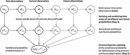
2.1.1. General Description

We present a Bayesian approach to combine multi-sensor optical and SAR time series for NRT deforestation detection. Figure 1 illustrates the main steps for applying the approach to multi-sensor time series, whereby we considered an NRT environment with past, current and future observations (Section 2.1.2). First (Step 1, Section 2.1.3), the conditional probabilities for non-forest are estimated for each individual time series observation, using the corresponding sensor specific probability density functions (pdfs) for forest (F) and non-forest (NF).

Secondly (Step 2, Section 2.1.4), observations at time t are flagged to be potentially deforested in the case that the conditional NF probability is larger than 0.5. For a flagged observation, the conditional probability of deforestation is computed by iterative Bayesian updating, using the previous observation (t − 1), the current observation (t), as well as i upcoming observations (t + i) to confirm or reject a deforestation event at t.

Figure 1. Schematic overview of the proposed Bayesian approach to fuse two multi-sensor time series and detect deforestation in near real-time. s1 and s2 refer to past, current and future time series observations from Sensor 1 (e.g., optical) and Sensor 2 (e.g., SAR), respectively.

Figure 1. Schematic overview of the proposed Bayesian approach to fuse two multi-sensor time series and detect deforestation in near real-time. s1 and s2 refer to past, current and future time series observations from Sensor 1 (e.g., optical) and Sensor 2 (e.g., SAR), respectively.

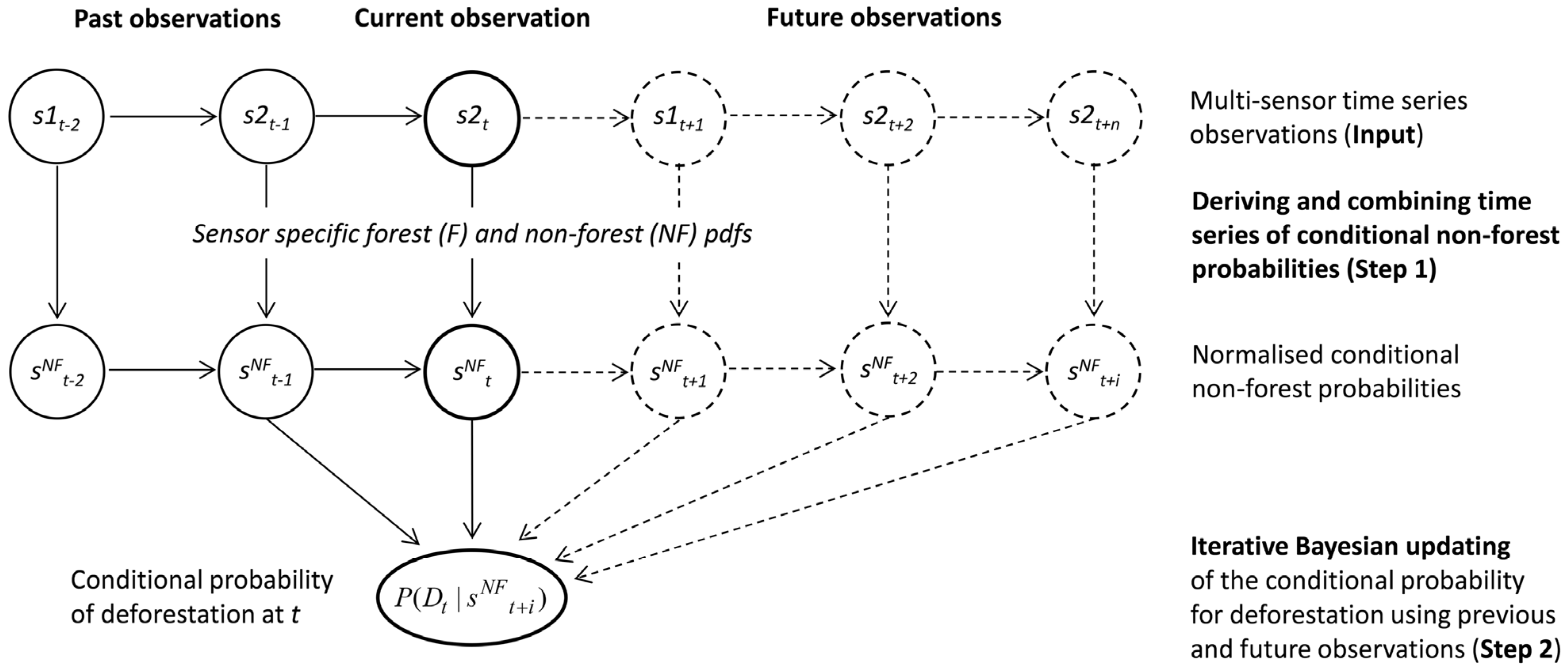
2.1.2. Multi-Sensor Time Series Observations (Input)

Let s1, ..., sn be discrete pixel time series derived from sensor 1, ..., sensor-n, where observations are non-equally spaced in time and observation times are non-identical between sensors. We can express the observation times of s1, ..., sn in the form T_s1 = {t^s1₁, t^s1_2, ..., t^s1_ks1} and T_sn = {t^sn₁, t^sn_2, ..., t^sn_ksn} with k_s1 and k_sn being the number of s1 and sn observations, respectively. Similarly, time series observations are denoted s1_t, ..., sn_t at t∊T_s1, ..., T_sn. Newly acquired observations are immediately processed and appended to the respective time series for NRT detection.

2.1.3. Deriving and Combining Time Series of Conditional NF Probabilities (Step 1)

Sensor-specific F and NF pdfs are fitted to F and NF training data using a maximum likelihood procedure. Next, the conditional probabilities of the time series observations, s1, given the presence of F and NF, p(s1|F) and p(s1|NF) are computed. According to the Bayes theorem and assuming equal priors for F and NF, the conditional NF probabilities P(NF|s1), are computed as follows:

$$P(NF|s{1}_t)=\frac{p(s{1}_t|NF)}{p(s{1}_t|NF)+p(s{1}_t|F)}fort\in T_{s1}$$

(1)

Since P(NF|s1) is later employed as new evidence for Bayesian updating, we want to avoid extreme probabilities, which would imply absolute certainty about either state F or NF. Therefore, we introduce a block weighting function that modifies the P(NF|s1) at 0.1 and 0.9. Defining P(NF|sn_t) analogously to P(NF|s1_t), the combined time series composed of conditional NF probabilities, s^NF is computed as:

$${s^{NF}}_t=\left\{\begin{array}{cc}P(NF|s{1}_t)& :t\in T_{s1}\\ ⋮& ⋮\\ P(NF|s{n}_t)& :t\in T_{sn}\end{array}\right\}$$

(2)

From here on, s^NF is considered to be the time series signal that is obtained from the sensors.

2.1.4. Iterative Bayesian Updating (Step 2)

Each new observation at time t is checked for potential deforestation and is assigned a flag λ = 1 if s^NF_t > 0.5 (potentially deforested) and a flag λ = 0 (not deforested) otherwise.

If λ_t = 1 at t = current, then the conditional probability of deforestation (D) at t is calculated using Bayesian probability updating [49] by taking the previous (t − 1) and the upcoming (t + i) signals, s^NF, into account:

$$P(D_t|{s^{NF}}_{t+i})=\frac{P({s^{NF}}_{t+i}|D)P(D_t|{s^{NF}}_{t+i-1})}{P({s^{NF}}_{t+i})}$$

(3)

with P(D_t|s^NF_t+i) being the posterior denoting the conditional probability of deforestation at t (D_t) given s^NF_t+i as new evidence and P(s^NF_t+i) being the total probability of the signal s^NF_t+i. i refers to the i-th future signal that can take values between i = 0,...,n.

For the initial step at (i = 0), the posterior P(D_t|s^NF_t) is calculated with the s^NF signal at the current step (s^NF_t) being the new evidence and the s^NF signal at the previous time step (s^NF_t-1) being the prior probability. In the subsequent steps (i > 0), the posterior P(D_t|s^NF_t+i) is repeatedly updated using upcoming s^NF signals (s^NF_t+i) as new evidence along with the posterior of the previous iteration as prior P(D_t|s^NF_t+i-1).

The iterative Bayesian updating is stopped and deforestation is detected in case P(D_t|s^NF_t+i) ≥ χ, with χ being a defined threshold. In case P(D_t|s^NF_t+i) decreases below 0.5 for a future signal (i > 0), we assume a false detection and set λ_t = 0. The next observation is then checked for potential deforestation.

2.2. Validation

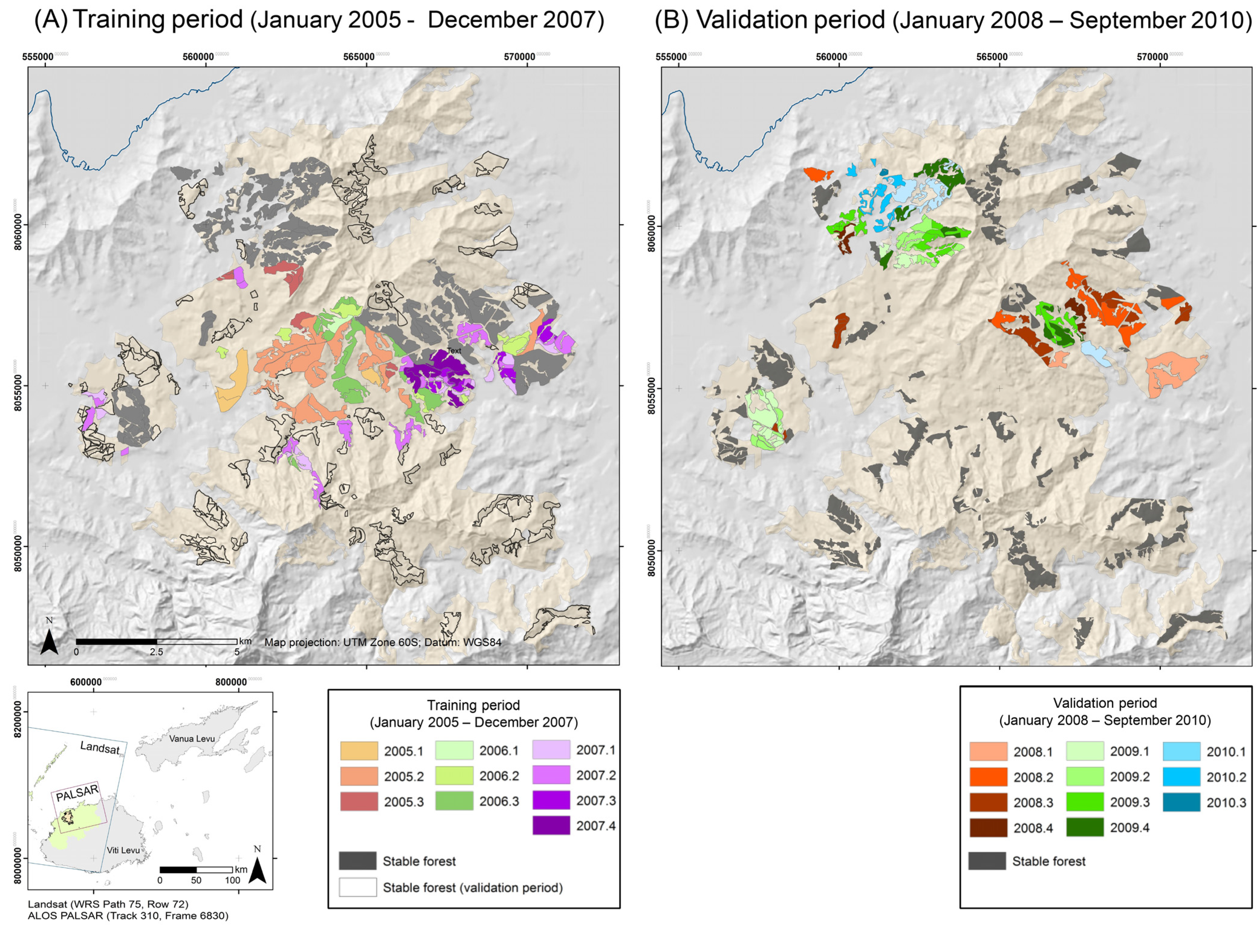
2.2.1. Study Area

We use an evergreen forest plantation in subtropical Fiji as our study area. The Lololo Fiji Pine Ldt. lease has been selected, because detailed spatial inventory data of 623 forest stands (Pinus caribaea) covering 9570 ha are available (Figure 2; latitude 17.32°S, longitude 177.37°E). The stand data comprises three-monthly (quarterly) harvesting information for 2000–2013 and replanting information for 1975–2013. The quarterly periods are denoted as 2008.1 and 2008.2 for the periods January 2008–March 2008 (day of year (DOY): 2008.1–2008.90) and April 2008–June 2008 (DOY: 2008.91–2008.181), respectively. The forest practice includes logging cycles of 15–20 years. Individual stands are deforested within a short period, and stems are removed quickly. Forest stands that remain unlogged for a period greater than 10 years after they have been replanted are covered with full-grown pine. For this study, we define a training period (January 2005–December 2007) and a validation period (January 2008–September 2010). During the training period, sensor-specific F and NF pdfs are derived to parameterize the proposed Bayesian approach to subsequently detect deforestation in the validation period. For both periods, separate forest masks were derived from the inventory data. The forest mask for the training period (Figure 2A) accounts for 3020 ha and includes forest stands planted before January 1995 and not logged before January 2005. Of those forest stands, 1464 ha were logged during the training period (January 2005–December 2007). The forest mask for the validation period (Figure 2B, January 2008–September 2010) accounts for 2859 ha and includes all forest stands planted before January 2000 and not logged before January 2008. Of those forest stands, 1395 ha were logged during the validation period, and 464 remained forest. Stable forest areas for the validation period do not overlap with the stable forest areas of the training period, ensuring an independent validation of the deforestation results (Figure 2A). In Figure 2A, stable forest areas of the validation period are overlaid with the training period dataset.

2.2.2. Landsat NDVI Data

All available 82 Level 1 Terrain (corrected) (L1T) Landsat 7 ETM+ images (quality: 9) for the Worldwide Reference System (WRS) Path 75 and Row 72 and acquired between January 2005 and September 2010 were used (Table 1). Landsat time series processing was performed as described in Reiche et al. [29]: Landsat images were processed individually using a standard processing chain consisting of Fmask (function of mask) [61] and LEDAPS (Landsat Ecosystem Disturbance Adaptive Processing System) [62,63,64]. Based on the uncorrected Landsat data in digital numbers, Fmask was used for masking clouds, cloud shadows and Landsat-7 SCL-off gaps as missing data. Using LEDAPS, atmospheric correction was performed to convert digital numbers to surface reflectance. Images were processed at 30-m spatial resolution and re-projected to WGS 84/UTM 60S.

Figure 2. The Lololo forest plantation, Fiji. Stable forest and logged forest stands with logging information at quarterly intervals are depicted for the training period ((A) January 2005–December 2007) and the validation period ((B) January 2008–September 2010). The stable forest areas of the validation area are also outlined for the training period. 2005.1 refers to the quarterly period January 2005–March 2005.

Figure 2. The Lololo forest plantation, Fiji. Stable forest and logged forest stands with logging information at quarterly intervals are depicted for the training period ((A) January 2005–December 2007) and the validation period ((B) January 2008–September 2010). The stable forest areas of the validation area are also outlined for the training period. 2005.1 refers to the quarterly period January 2005–March 2005.

Table 1. Frequency by year of the Landsat 7 ETM+ (WRS Path 75, Row 72) and ALOS PALSAR Fine Beam Dual (FBD) (Track 310, Frame 6830) observations for 2005–September 2010.

	Training Period			Validation Period
Year	2005	2006	2007	2008	2009	September 2010
No. of Landsat images	12	14	13	16	14	13
No. of ALOS PALSAR FBD images	-	-	3	3	1	2

Table 1. Frequency by year of the Landsat 7 ETM+ (WRS Path 75, Row 72) and ALOS PALSAR Fine Beam Dual (FBD) (Track 310, Frame 6830) observations for 2005–September 2010.

	Training Period			Validation Period
Year	2005	2006	2007	2008	2009	September 2010
No. of Landsat images	12	14	13	16	14	13
No. of ALOS PALSAR FBD images	-	-	3	3	1	2

As described in Reiche et al. [29], per-pixel missing data (MD) was calculated based on the processed NDVI stack. MD varies from 35% to 69% and averages 53% for the validation area. We increased the per-pixel percentage of MD from an average of 53% for the original (org) Landsat time series stack to 70%, 80%, 90% and 95% by randomly excluding observations on a pixel basis. The approximate number of per-pixel Landsat observations per year ranges from 6.5 to 0.6 observations/year for 53% (org) and 95% MD, respectively (Table 2).

Table 2. Approximate number of per-pixel observations per year for the original (org, mean 53%) Landsat NDVI time series and for Landsat NDVI time series with 70%, 80%, 90% and 95% missing data (MD).

Per-Pixel MD	Approximate Number of Per-Pixel Observations Per Year
No MD (0%)	12.3
org (35%–69%) (mean 53%)	3.8–9.25 (mean 6.5)
70%	3.8
80%	2.5
90%	1.2
95%	0.6

Table 2. Approximate number of per-pixel observations per year for the original (org, mean 53%) Landsat NDVI time series and for Landsat NDVI time series with 70%, 80%, 90% and 95% missing data (MD).

Per-Pixel MD	Approximate Number of Per-Pixel Observations Per Year
No MD (0%)	12.3
org (35%–69%) (mean 53%)	3.8–9.25 (mean 6.5)
70%	3.8
80%	2.5
90%	1.2
95%	0.6

2.2.3. ALOS PALSAR Data

All ALOS PALSAR images (Track 310; Frame 6830) in Fine Beam Dual (FBD) mode [65] were acquired for the period between 2007 and 2010 (Table 1). The time series consists of 9 Level 1.1 dual-polarized FBD images (HH and HV polarization) in ascending mode with an incidence angle of 34.3°. Time series pre-processing was done as described in Reiche et al. [29]: Using the Gamma software package [66], pre-processing was performed independently for each image, including multi-looking, radiometric calibration using standard calibration coefficients [67], topographic normalization as described by [68] and geocoding to 25-m pixel resolution (WGS84, UTM 60S) using a local 30-m DEM. Geocoding includes an automated cross-correlation between the SAR image and a simulated SAR image that was derived from the DEM in a first step. The cross-correlation results in the range and azimuth offset-polynomial sub-pixel accuracy that is used for geocoding the SAR image in the last step [66]. The geocoding accuracy was found to be below 0.5 pixels for all images.

The individual HH and HV images were stacked and subsequently resampled to the 30-m Landsat pixel cells using nearest-neighbor interpolation. Overlapping pixels with the same spatial resolution are required to fuse at the pixel level. By subtracting the HV and HH backscatter time series, an HVHH backscatter ratio time series was derived (HVHH). In addition to the general SAR pre-processing steps, adaptive multi-temporal SAR filtering [69] was applied to the time series stacks. The multi-temporal filtered backscatter time series are hereafter referred to as HH_mt, HV_mt and HVHH_mt. A more detailed description of the pre-processing can be found in [29].

For the remaining analysis, we only considered HVHH_mt, as previous results have shown that the HVHH polarization ratio is more sensitive to deforestation than HH or HV [29,70]. This may be explained by the fact that the ratio of HV and HH partially compensates for environmental effects, such as changing moisture conditions [29]. Increasing moisture over forest and open areas after a rainfall event, for example, leads to an increase in the backscatter for both HV and HH [71].

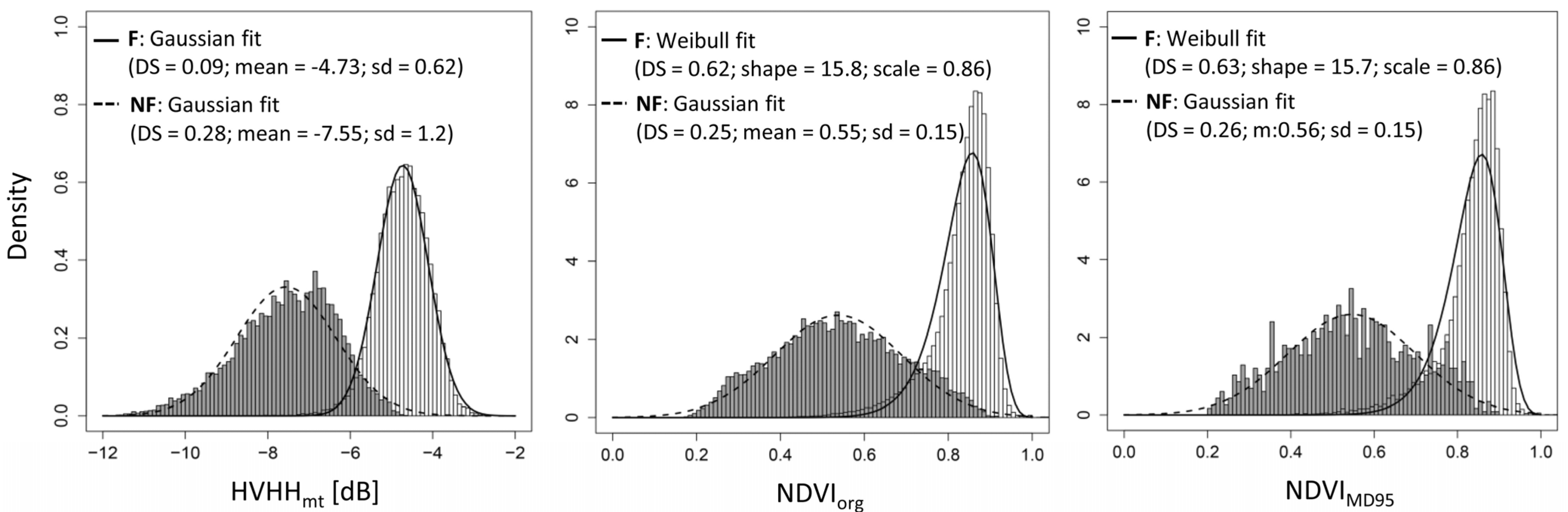
2.2.4. Deriving F and NF pdfs

F and NF distributions were derived separately for Landsat NDVI_MD (MD = org, 70%, 80%, 90% and 95%) and ALOS PALSAR HVHH_mt using stable forest and change areas in the training period. To derive F distributions, all time series observations covered by stable forest were considered. To derive the NF distribution, only time series observations acquired at NF conditions immediately after deforestation events were used. To account for the precision of the reference data (0.25 years), only observations acquired from 0.25 to 0.75 years after logging were considered. During this period, NF conditions can be expected, even in the case of immediate replanting. We considered observations acquired during the entire year to derive F and NF distributions. Because of the low observation frequency of medium resolution Landsat (~6.5 observations/year) and PALSAR (~2 observations/year), a situation commonly encountered in most tropical regions, only marginal seasonality of evergreen forest is visible. Therefore, we assumed non-seasonality over stable forest, which is justified by other studies [21,72] and previous work using the same dataset [29].

Images affected by remaining clouds over F and NF training areas as a result of an imperfect cloud mask [22,28,61] that would bias the distributions were removed manually. Twelve of the 39 images available for the training period were removed. We evaluated the separability of the F and NF distributions for NDVI_MD and HVHH_mt using the normalized Jeffries-Matusita distance (JM) [73]. JM has a finite dynamic range from 0 (inseparable) to 2 (separable).

A model was fitted separately to each of the derived univariate F and NF distributions by maximum-likelihood fitting using an iterative optimization method [74]. Gaussian, Gamma and Weibull models were tested and the Kolmogorov–Smirnov (K-S) test was used for assessing goodness of fit [75]. The K-S test D-statistics indicate the maximum distance between the cumulative pdfs to the modelled distribution and the sample distribution. The model resulting in the lowest D-statistic was selected. The K-S test is available in the stats package for R.

2.2.5. Detecting Deforestation in an NRT Scenario

To validate the method for NRT deforestation detection, we emulated a NRT scenario for the validation period. From the start of the validation period (January 2008) onwards, individual NDVI_MD and HVHH_mt observations were added chronologically to the time series until the end of the validation period (September 2010). For detecting deforestation, the approach was applied to each newly-added observation. Subsequent observations were handled as future observations. The output for each time step is a deforestation map showing the conditional probability of deforestation for unconfirmed changes (soft information) and the time of change for confirmed changes (hard information).

First, we analyzed the single-sensor results for increasing χ from χ = 0 to χ = 1 in steps of 0.025 and compared them for HVHH_mt and NDVI_org. In addition, we analyzed $\overline{n}$, the mean number of future observations used to confirm the change (n). Based on these results, simple rules were defined for the fused NDVI_MD-HVHH_mt case with which we aimed for a high overall accuracy (OA) and rapid detection of change. We applied the same rules to NDVI_MD-only and HVHH_mt-only and fused NDVI_MD-HVHH_mt cases and compared them for increasing MD.

We assessed both the spatial and temporal accuracy of the detected deforestation by following Reiche et al. [29]. Spatial accuracy was defined as the overall accuracy, which is inversely related to omission and commission errors of detected changes. The temporal accuracy refers to the extent to which timing of the detected changes are correct. Available reference data that covers the entire study area allowed a map comparison. A major advantage of map comparison compared to common probabilistic sampling methods is that no sampling errors are introduced [76], since the number of pixels in the deforestation map represents the sample unit. To account for mixed pixels on the edges of the reference polygons, we only included a pixel if at least two-thirds of the pixel covers the reference polygon. To assess the spatial accuracy, a confusion matrix was derived [77,78,79] from the deforestation and no-change class. We calculated the OA, the omission error (OE) and commission error (CE) of the deforestation class following [79].

Temporal accuracy was assessed by calculating the mean time-lag between the time at which correctly detected changes were initially flagged (MTL_F) and the time at which the change was confirmed (MTL). For each correctly detected change pixel, the time at which the change was first flagged (T_F) and the time at which it was confirmed (T) were converted to quarterly periods, after which the time differences with the validation data were calculated. The MTL_F and MTL were calculated as the mean of the time differences of all correctly detected change pixels and was given in months. The MTL_F provides the time lag until change events are indicated and allows identification of early detections. It is important to analyze the MTL_F and MTL jointly with the OE, because MTL_F and MTL are calculated based on correctly detected changes only.

3. Results

3.1. Deriving F and NF pdfs

Figure 3 depicts the F and NF distributions for HVHH_mt, NDVI_org and NDVI_MD95 overlaid with fitted pdfs. HVHH_mt was found to have the highest F-NF class separability (JM = 1.39) when compared to NDVI_org (JM = 1.17) and NDVI_MD95 (JM = 1.13). The K-S test D-statistics (DS) indicated a Gaussian model as the best fit for the HVHH_mt F and NF distributions, as well as for the NDVI_org and NDVI_MD95 NF distributions.

Figure 3. HVHH_mt, NDVI_org and NDVI_MD95 distributions for F (dark grey) and NF (light grey) overlaid with the modelled pdfs. The Kolmogorov-Smirnov (K-S) test D-statistics (DS) of the fitted distribution models are given. The mean and standard deviation (sd) of the Gaussian fit and shape and scale parameter of the Weibull fit are given.

Figure 3. HVHH_mt, NDVI_org and NDVI_MD95 distributions for F (dark grey) and NF (light grey) overlaid with the modelled pdfs. The Kolmogorov-Smirnov (K-S) test D-statistics (DS) of the fitted distribution models are given. The mean and standard deviation (sd) of the Gaussian fit and shape and scale parameter of the Weibull fit are given.

For NDVI_org and NDVI_MD95 F distributions, a Weibull model resulted in the best fit for distributions with DS slightly below the DS for a Gaussian model (DS = 0.62 for the Weibull model vs. DS = 0.65 for the Gaussian model). Figure 3 also provides the mean and standard deviation (sd) describing the Gaussian pdfs and the shape and scale parameter describing the Weibull pdfs. The derived parameter for NDVI_org and NDVI_MD95 were found to be consistent for increasing MD. Thus, we used the parameters found for NDVI_org for all MD.

3.2. Detecting Deforestation in an NRT Scenario

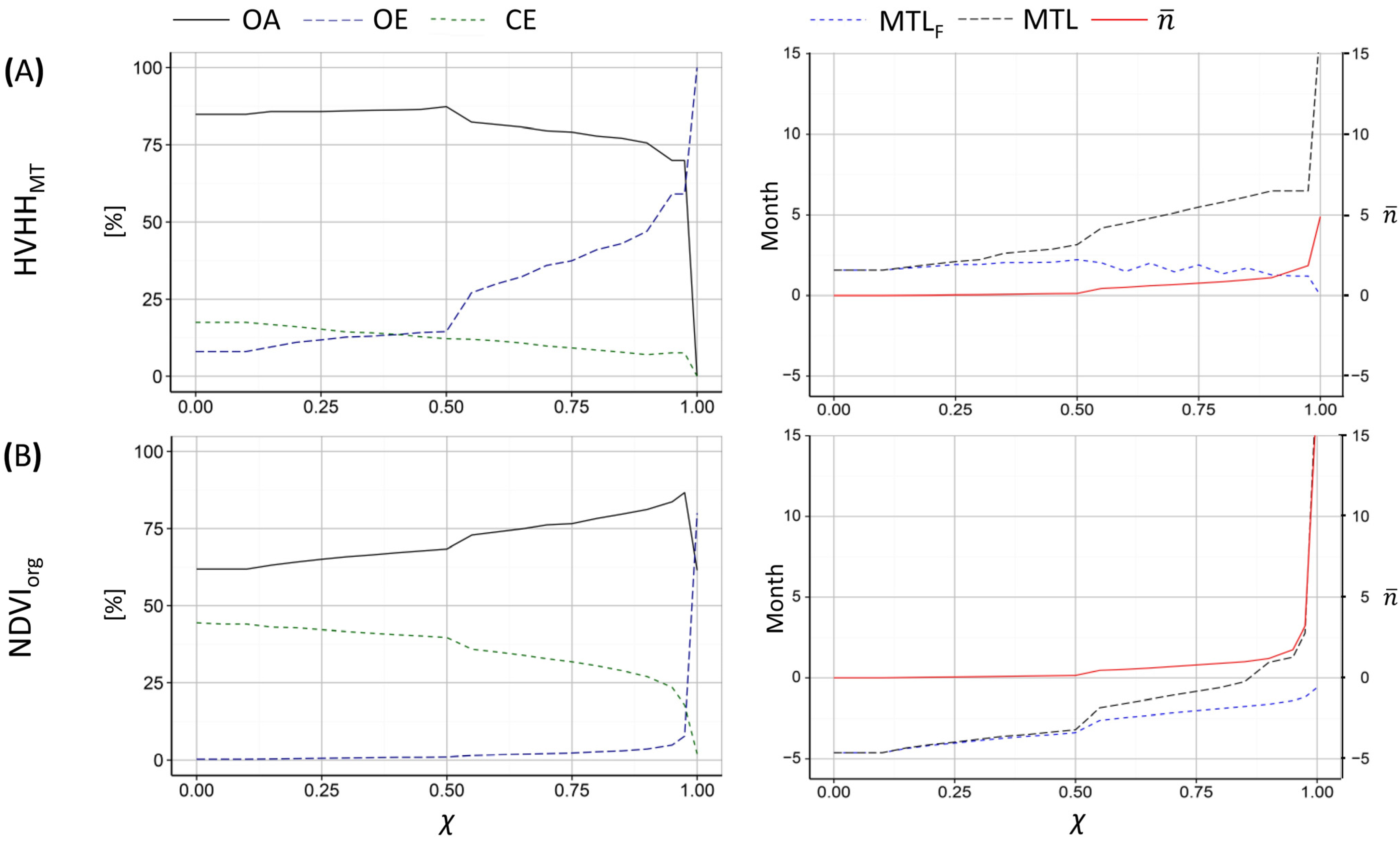
3.2.1. Single-Sensor Results for Increasing the χ Threshold

Figure 4 shows the spatial accuracy (OA, OE, CE) and the temporal accuracy (MTL_F, MTL), as well as $\overline{n}$ as a function of χ, separately for HVHH_mt and NDVI_org. The results can be summarized as follows. For both HVHH_mt and NDVI_org, an increasing χ was observed to result in a decreasing CE and an increasing OE, MTL_F, MTL and $\overline{n}$.

Figure 4. Spatial accuracy (OA, overall accuracy; OE, omission error; CE, commission error), temporal accuracy (MTL_F, mean time lag of flagged changes; MTL, mean time lag of confirmed changes) and the mean number of future observations used to confirm a deforestation event ($\overline{n}$) as a function of χ, separately for HVHH_mt (A) and NDVI_org (B).

Figure 4. Spatial accuracy (OA, overall accuracy; OE, omission error; CE, commission error), temporal accuracy (MTL_F, mean time lag of flagged changes; MTL, mean time lag of confirmed changes) and the mean number of future observations used to confirm a deforestation event ($\overline{n}$) as a function of χ, separately for HVHH_mt (A) and NDVI_org (B).

For HVHH_mt (Figure 4A), the OA was found to slightly increase with increasing χ from χ = 0 and was highest for χ = 0.5 (OA = 87.3%, OE = 14.5%, CE = 12.2%). For χ = 0.5, an MTL_F and an MTL of 2.2 and 3.2 months were observed, respectively, and $\overline{n}$ was found to be 0.12. For increasing χ > 0.5, the OA decreases consistently.

For NDVI_org (Figure 4B), the OA was observed to consistently increase with increasing χ and was highest for χ = 0.975 (OA = 86.7, OE = 7.8%, CE = 17.8%). For χ > 0.975, the OA dropped due to a strongly increasing OE. At χ = 0.975, an MTL_F and an MTL of −1.2 and 2.8 months, respectively, were observed, and $\overline{n}$ was found to be 1.75. The MTL_F was observed to increase from −4.6 to −1.2 months with increasing values of χ from zero to 0.975, respectively. While an MTL_F of −1.2 months is within the precision of the reference data (±1.5 months), lower values clearly reflect an early detection, which is confirmed by a high CE. Early detections can be explained by spectral variations in the NDVI time series and remaining clouds resulting in low NDVI values. The results show that using a fixed value for χ does not lead to consistent results for HVHH_mt and NDVI_org when aiming for the highest OA.

The highest OAs were found for a χ for which the OE and CE are approximately equal, meaning that on the whole, the map is unbiased. The changes in spatial and temporal accuracies for increasing χ strongly depend on the time series metrics and their observation density and stability over time. Based on the findings described above and aiming for the highest OA, the following simple rules were defined for the fused NDVI_MD-HVHH_mt case. We used χ = 0.5 for new HVHH_mt observations and χ = 0.975 for new NDVI_MD observations. In addition, a deforestation label was only assigned if s^NF > 0.5 was found given the new observation. We applied the same rules to NDVI_MD and HVHH_mt and fused NDVI_MD-HVHH_mt cases and compared them for increasing MD. The results are presented in the following section.

3.2.2. Multi-Sensor Results

Figure 5 shows the spatial accuracy (OA, OE, CE) and the temporal accuracy (MTL_F, MTL) as a function of MD for the NDVIMD-only, HVHHmt-only and fused NDVIMD-HVHHmt cases. The accuracy assessment results can be summarized as follows:

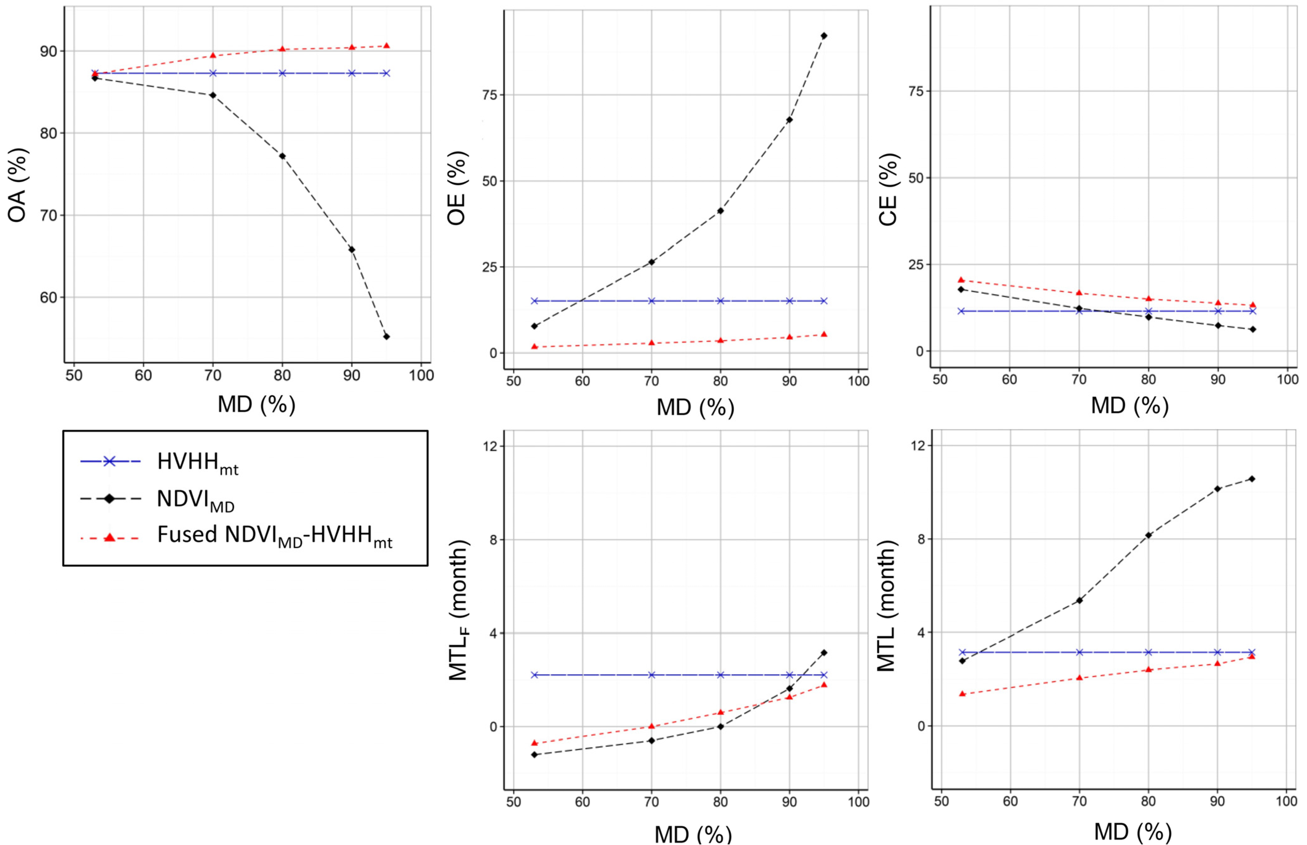
• For HVHHmt-only, the results are identical to the results observed for χ = 0.5 and outlined in the previous section (OA = 87.3%, OE = 14.5%, CE = 12.2%, MTL_F = 2.2 months, MTL = 3.2 months).
• For NDVI_MD-only, a strong decrease in the spatial and temporal accuracy was observed with increasing MD. Compared to HVHHmt-only, a slightly lower spatial accuracy (OA = 86.7%, OE = 7.8%, CE = 17.8%) was observed for MD = org. The OA dropped from 86.7% for MD = org to 55.2% for MD = 95, mainly due to increasing omitted changes. For MD = 95, the OE reached 92.2%, and the CE slightly decreased to 6.3%. The strong reduction of the observation density with increasing MD led to a strong decrease in temporal accuracy. The MTL_F dropped from −1.2 (MD = org) to 3.2 months (MD = 95), and the MTL decreased from 2.8 (MD = org) to 10.6 months (MD = 95).
• For fused NDVIMD-HVHHmt, an improved spatial and temporal accuracy was found compared to NDVI_MD- and HVHH_mt-only. The MTL_F and MTL decreased from −0.7 and 1.3 months (MD = org) to 1.8 and 2.9 months (MD = 95). The OA was found to increase for increasing MD from 87.4% (MD = org) to 90.4% (MD = 95) due to a decreased CE, as a result of the decreasing influence of the NDVI_MD on the results. Though the CE is lower when compared to NDVI_MD-only and decreased from 20.4% (MD = org) to 13.2% (MD = 95), it was higher when compared to HVHH-only (CE = 12.2%). The OE improved compared to both single-sensor results due to an increased observation density and was found to be only 1.7% for MD = org and slightly increased to 5.3% for MD = 95%.

Figure 5. Spatial accuracy and temporal accuracy for NDVI_MD-only, HVHH_mt-only and fused NDVI_MD-HVHH_mt as a function of NDVI per-pixel MD.

Figure 5. Spatial accuracy and temporal accuracy for NDVI_MD-only, HVHH_mt-only and fused NDVI_MD-HVHH_mt as a function of NDVI per-pixel MD.

Figure 6 illustrates the map results for the HVHH_mt-only, NVDI_org-only and NDVI_MD95-only cases compared to the fused NDVI_org-HVHH_mt case and fused NDVI_MD95-HVHH_mt case, respectively. Due to the strong contribution of both NDVI_org and HVHH_mt time series used for the fused NDVI_org-HVHH_mt case, the map results appear to be a combination of both, showing areas where deforestation is detected earlier when compared to HVHH_mt-only (red circles) and NDVI_org-only (blue circles), respectively. Yellow circles in Figure 6 indicate areas of unconfirmed deforestation for the HVHH_mt-only case that are confirmed in the fused NDVI_org-HVHH_mt case due to an increased number of observations. This explains the decreased OE for the fused case when compared to the single-sensor results. The NDVI_MD95-HVHH_mt case appears almost identical to the HVHH_mt-only case due to the sparse contribution of NDVI_MD95.

To better illustrate how the single-sensor time series are used complimentarily to improve monitoring of deforestation in NRT when using the proposed approach, Figure 7 shows a sequence of quarterly deforestation maps over a subset of the study area for the year 2008 separately for NDVI_org-only (A), HVHH_mt-only (B) and fused NDVI_org-HVHH_mt (C). For each time step, the MTL and the conditional probability of deforestation for unconfirmed changes are given. Comparing the quarterly map results for NDVI_org-only (Figure 7A–D) and HVHH_mt-only revealed that changes are flagged much earlier due to the dense observation density of NDVI_org, but often are confirmed later.

Figure 6. (A) Reference data. Map results showing detected deforestation from January 2008 to September 2010 for HVHH_mt-only (B), NDVI_org-only (C) compared to fused NDVI_org-HVHH_mt (D), and NDVI_MD95-only (E) compared to fused NDVI_MD95-HVHH_mt (F). Encircled areas indicate where deforestation was detected earlier for the fused NDVI_org-HVHH_mt when compared to HVHH_mt-only (red circles) and NDVI_org-only (black circles), respectively. Yellow circles: detected deforestation for the fused NDVI_org-HVHH_mt, but not confirmed for HVHH_mt-only.

Figure 6. (A) Reference data. Map results showing detected deforestation from January 2008 to September 2010 for HVHH_mt-only (B), NDVI_org-only (C) compared to fused NDVI_org-HVHH_mt (D), and NDVI_MD95-only (E) compared to fused NDVI_MD95-HVHH_mt (F). Encircled areas indicate where deforestation was detected earlier for the fused NDVI_org-HVHH_mt when compared to HVHH_mt-only (red circles) and NDVI_org-only (black circles), respectively. Yellow circles: detected deforestation for the fused NDVI_org-HVHH_mt, but not confirmed for HVHH_mt-only.

Figure 7. Time sequence showing quarterly deforestation maps for 2008 for NDVI_org-only ((A) A1–A4), HVHH_mt-only ((B) B1–B4) and fused NDVI_org-HVHH_mt ((C) C1–C4). The reference map is given in (D4) (D). For each time step, the detected deforestation (MTL) and the conditional probability of deforestation (deforestation probability) for unconfirmed changes is given.

Figure 7. Time sequence showing quarterly deforestation maps for 2008 for NDVI_org-only ((A) A1–A4), HVHH_mt-only ((B) B1–B4) and fused NDVI_org-HVHH_mt ((C) C1–C4). The reference map is given in (D4) (D). For each time step, the detected deforestation (MTL) and the conditional probability of deforestation (deforestation probability) for unconfirmed changes is given.

Although deforestation was already flagged at 2008.1 (A1), it was not confirmed until 2008.3 (A3). For HVHH_mt, in contrast, deforestation was not flagged in 2008.1 (B1), but already confirmed in 2008.2 (B2). The fused results combine the advantages of both NDVI_org and HVHH_mt with deforestation events being flagged early and also confirmed early. As a result, deforestation is flagged in 2008.1 (C1) and confirmed in 2008.2 (C2).

Figure 8 and Figure 9 illustrate two single-pixel examples showing the original NDVI_org and HVHH_mt time series (top) and the combined time series of conditional NF probabilities, s^NF (bottom). Figure 8 shows a time series where deforestation was detected, with the deforestation confirmed (T = 2008.266 (DOY)) shortly after it has been flagged (T_F = 2008.219 (DOY)). A remaining cloud at the beginning of 2008 was flagged as possible deforestation, but not confirmed. Figure 9 shows a committed change. Since the forest seems to be disturbed and not stable at a high NDVI level as seen for the previous pixel example (Figure 8) and typical for evergreen tropical forest, s^NF varies strongly, which causes a committed change. It should be noted that HVHH_mt does not show these fluctuations, and in the HVHH_mt-only results, no change was detected. This explains the higher CE found for the fused results when compared to HVHH_mt-only.

Figure 8. Pixel example showing correctly detected deforestation for the fused NDVI_org-HVHH_mt case. The NDVI_org and HVHH_mt time series (top) and the conditional NF probabilities, s^NF (bottom), are shown. The time at which the change was first flagged (T_F) and the time at which it was confirmed (T) are given.

Figure 8. Pixel example showing correctly detected deforestation for the fused NDVI_org-HVHH_mt case. The NDVI_org and HVHH_mt time series (top) and the conditional NF probabilities, s^NF (bottom), are shown. The time at which the change was first flagged (T_F) and the time at which it was confirmed (T) are given.

Figure 9. Pixel example showing commission error in change detection for the fused NDVI_org-HVHH_mt case. The NDVI_org and HVHH_mt time series (top) and the conditional NF probabilities, s^NF (bottom), are shown. The time at which the change was first flagged (T_F) and the time at which it was confirmed (T) are given.

Figure 9. Pixel example showing commission error in change detection for the fused NDVI_org-HVHH_mt case. The NDVI_org and HVHH_mt time series (top) and the conditional NF probabilities, s^NF (bottom), are shown. The time at which the change was first flagged (T_F) and the time at which it was confirmed (T) are given.

4. Conclusions

Providing deforestation information in NRT and at medium-resolution scale can provide a powerful tool for governments and forestry stakeholders to improve the management and conservation of forest resources. We presented a Bayesian approach to combine optical and SAR time series for NRT deforestation detection. We applied the approach to univariate Landsat NDVI and ALOS PALSAR HVHH_mt backscatter time series imagery and detected deforestation from January 2008–September 2010 in an NRT scenario in an evergreen plantation forest in the tropics. Once a new image of either of the input time series was available, it was immediately used as new evidence to update the probability for deforestation and to confirm or reject a possible deforestation event. To the best knowledge of the author of this article, for the first time, an optical-SAR time series fusion approach designed for NRT deforestation detection that exploits the entire temporal detail has been introduced.

Evaluating the results with three-monthly reference data revealed that fusing NDVI_MD and HVHH_mt always improved the spatial and temporal accuracy of single-sensor systems, even for increasing Landsat MD. For the NDVI-only case, instead, a very strong decrease in spatial and temporal accuracy was observed for increasing MD percentage. The results confirm the trends observed by Reiche et al. [29] and emphasizes once more the weakness of tropical forest monitoring efforts relying on optical data only. Combining time series observations from Landsat and PALSAR increased the observation density and helped to mitigate the problem of missing data in optical (frequent cloud cover) and SAR time series (limited observation frequency). Due to the consistent PALSAR time series of ~2 observations/year, fusing even improved the results in the case of very few available Landsat observations (MD = 95%; 0.5 observations/year).

Reiche et al. [29] presented results for the same dataset and validation period (January 2008–September 2010), using MulTiFuse (see Section 1) to fuse NDVI_MD and HVHH_mt time series. A non-parametric time series analysis method was used (BFAST-monitor, [27]) for detecting historical deforestation. In contrast to the current study, where an NRT scenario was emulated, the entire time series was available from the beginning (historical scenario). Although the methods are not entirely comparable, the following differences are evident when comparing the results obtained for MulTiFuse [29] and the Bayesian approach (this study). A higher OA was obtained for MulTiFuse when compared to the Bayesian approach. The higher OA as a result of less committed changes observed for MulTiFuse can be explained by the fact that the entire time series was available from the beginning. This allowed considering the entire time series variability when applying BFAST-monitor to detect deforestation. For the Bayesian approach, however, less omitted changes and an improved temporal accuracy were found. Since MulTiFuse requires observations from both before and after the change events in both time series for fusion, deforestation will be detected with a larger delay. In fact, a much weaker MTL is expected when applying MulTiFuse in NRT. These results indicate that satellite-based monitoring systems are limited to satisfying the requirements for both the reliable assessment of historical changes and NRT monitoring. While MulTiFuse was shown to be more suitable for monitoring historical deforestation, the Bayesian approach highlighted its capabilities for NRT deforestation detection.

Initial results from the HVHH_mt- and NDVI_MD-only time series for increasing χ confirmed the results of previous studies [39], which showed that the CE is always a compromise with the OE. In the same manner, an increasing MTL results in a decreased CE and increased OE as a result of more observations used to confirm a deforestation event. Using a sensor-specific χ for the fused case enabled us to account for the characteristics of the different time series observations of NDVI_MD and HVHH_mt. A χ = 0.975 resulted in the highest OA for NDVI_org, showing that a high confidence linked to a high number of future observations ($\overline{n}$ = 1.75) is needed to confirm a possible deforestation event using NDVI_org-only. Remaining clouds and a rather strong varying spectral signal over time does result in false detection when using a lower χ. In contrast, χ = 0.5 was found to result in the highest OA for HVHH_mt-only (OA = 87.3%), exceeding the OA for NDVI_org-only. Only a very small number of observations are required to confirm a deforestation event ($\overline{n}$ = 0.12), showing the stability of the HVHH_mt time series signal over evergreen tropical forest. These findings confirm the results of many studies showing the capabilities of L-band backscatter for detecting tropical deforestation [29,34,38].

In this study, we deal with a forest practice in which stands are being harvested within a short period and stems are removed immediately after logging. The existence of such regimented harvesting practices, in combination with the availability of three-monthly reference data covering the entire study area, greatly reduced the number of unknowns, providing an ideal situation for assessing the performance of the introduced approach. For operational use, however, the approach needs to be applied and tested for varying harvesting practices and more complex forest dynamics. In the present case and common to deforestation in tropical evergreen forest, the removal of forest causes a large drop in the HVHH_mt signal. This is confirmed by two clearly separated distributions found for F and NF. In the case of other forest practices, for example when fallen logs are left after logging [33,39], causing an initial increase of the signal, a second NF distribution should be added.

We demonstrated the derivation of F and NF distributions from univariate time series. In order to make use of the available reflectance and backscatter spectra of optical and SAR, class distributions should be derived from multivariate time series. Using all available Landsat bands and other metrics (e.g., Landsat Band 5 or band 7, normalized burn ratio, tasseled cap wetness, texture), for example, showed improved F and NF class distinction [21,44,80,81].

Providing a combination of spatially-explicit hard and soft information, namely the time of change of confirmed changes and the conditional probability of deforestation for indicated changes, is considered one of the major advantages of a probabilistic framework [50,51,82]. A disadvantage of probabilistic approaches when compared to non-parametric approaches is the need for training data to derive class-specific distributions [68], such as in our case for F and NF. However, satellite-based medium-resolution optical (Landsat), as well as C- (ERS-1, ENVISAT ASAR) and L-band SAR imagery (JERS-1, ALOS PALSAR) is available for most areas of the world. While Broich et al. [83] demonstrated the derivation of time series of forest probabilities from Landsat time series for Sumatra and Kalimantan, Shimada et al. [37] successfully demonstrated the extraction of F and NF distributions for PALSAR across global biomes using globally-distributed F and NF reference areas. An approach to automatically extract the required F and NF reference areas on the basis of Landsat imagery has been introduced by Huang et al. [84].

The proposed probabilistic approach is designed to combine time series observations from multiple SAR and optical sensors. Because conditional NF probabilities are used to calculate and update the conditional probability of deforestation, the approach directly accounts for the different sensor-specific class separability. This is of particular interest when making use of C-band SAR time series from ESA’s Sentinel-1 in combination with L-band and Landsat. The lower sensitivity of C-band to deforestation when compared to L-band [85] is expected to result in more overlapping class F and NF distributions used to compute conditional NF probabilities (Equation (1)) and, thus, less extreme class NF probabilities. A reduced impact of single C-band observations on the conditional probability of deforestation will be the result; however, this may partly be compensated by an increased observation frequency expected for Sentinel-1 [86]. Combining the impending streams of medium-resolution optical (Landsat and Sentinel-2), C-band SAR (Sentinel-1) and L-band SAR data (SAOCOM and ALOS-2 PALSAR-2) has the potential to further advance NRT deforestation monitoring efforts. Even challenges, such as irregular seasonal cloud cover, sudden discontinuity from a satellite due to sensor failure or unexpected changes in data policy, may be compensated.

References

- Assunção, J.; Gandour, C.; Rocha, R. DETERring Deforestation in the Brazilian Amazon: Environmental Monitoring and Law Enforcement. Available online: http://www.econ.puc-rio.br/uploads/adm/trabalhos/files/DETERring-Deforestation-in-the-Brazilian-Amazon-Environmental-Monitoring-and-Law-Enforcement-Technical-Paper.pdf (accessed on 17 March 2015).
- Lynch, J.; Maslin, M.; Balzter, H.; Sweeting, M. Choose satellites to monitor deforestation. Nature 2013, 496, 293–294. [Google Scholar] [CrossRef] [PubMed]
- Nellermann, C. Green Carbon, Black Trade: Illegal Logggin, Tax Fraud and Laundering in the Worlds Tropical Forests. A Rapid Response Assessment. Available online: http://www.unep.org/pdf/RRAlogging_english_scr.pdf (accessed on 17 March 2015).
- “Illegal” Logging and Clobal Wood Markets: The Competitive Impacts on the U.S. Wood Products Industry, Prepared for American Forest & Paper Association by Seneca Creek Associates and Wood Resources International. 2004.
- Masiero, M.; Secco, L.; Pettenella, D.; Brotto, L. Standards and guidelines for forest plantation management: A global comparative study. For. Policy Econ. 2015, 53, 29–44. [Google Scholar] [CrossRef]
- FAO. Global Forest Resource Assessment 2010. Main Report; Forest Resources Devision, FAO: Rome, Italy, 2010. [Google Scholar]
- Hammer, D.; Kraft, R.; Wheeler, D. Alerts of forest disturbance from MODIS imagery. Int. J. Appl. Earth Obs. Geoinf. 2014, 33, 1–9. [Google Scholar] [CrossRef]
- Wheeler, D.; Hammer, D.; Kraft, R.; Steele, A. Satellite-Based Forest Clearing Detection in the Brazilian Amazon: FORMA, DETER, and PRODES; World Resources Institute: Washington, DC, USA, 2014. [Google Scholar]
- Hansen, M.; Potapov, P.; Moore, R.; Hancher, M.; Turubanova, S.A.; Tyukavina, A.; Thau, D.; Stehman, S.V.; Goetz, S.J.; Loveland, T.R.; et al. High-resolution global maps of 21st-century forest cover change. Science 2013, 342, 850–853. [Google Scholar] [CrossRef] [PubMed]
- Shimabukuro, Y.E.; Duarte, V.; Anderson, L.O.; Valeriano, D.M.; Arai, E.; Freitas, R.M.D; Rudorff, B.F.T.; Moreira, A.A. Near real time detection of deforestation in the Brazilian Amazon using MODIS imagery. Rev. Ambient. Agua An Interdiscip. J. Appl. Sci. 2006, 1, 37–47. [Google Scholar] [CrossRef]
- Hammer, D.; Kraft, R.; Wheeler, D. FORMA: Forest Monitoring for Action-Rapid Identification of Pan-Tropical Deforestation Using Moderate-Resolution Remotely Sensed Data; Centre for Global Development: Rochester, NY, USA, 2009. [Google Scholar]
- Anderson, L.O.; Shimabukuro, Y.E.; DeFries, R.S.; Morton, D. Assessment of deforestation in near real time over the Brazilian Amazon using multitemporal fraction images derived from Terra MODIS. IEEE Geosci. Remote Sens. Lett. 2005, 2, 315–318. [Google Scholar] [CrossRef]
- Tyukavina, A.; Stehman, S.V; Potapov, P.V; Turubanova, S.A; Baccini, A.; Goetz, S.J.; Laporte, N.T.; Houghton, R.A; Hansen, M.C. National-scale estimation of gross forest aboveground carbon loss: A case study of the Democratic Republic of the Congo. Environ. Res. Lett. 2013, 8, 044039. [Google Scholar] [CrossRef]
- Achard, F.; Beuchle, R.; Mayaux, P.; Stibig, H.-J.; Bodart, C.; Brink, A.; Carboni, S.; Desclée, B.; Donnay, F.; Eva, H.D.; et al. Determination of tropical deforestation rates and related carbon losses from 1990 to 2010. Glob. Chang. Biol. 2014, 20, 2540–2054. [Google Scholar] [CrossRef] [PubMed]
- DeVries, B.; Verbesselt, J.; Kooistra, L.; Herold, M. Robust monitoring of small-scale forest disturbances in a tropical montane forest using Landsat time series. Remote Sens. Environ. 2015, 161, 107–121. [Google Scholar] [CrossRef]
- Griffiths, P.; Kuemmerle, T.; Baumann, M.; Radeloff, V.C.; Abrudan, I.V.; Lieskovsky, J.; Munteanu, C.; Ostapowicz, K.; Hostert, P. Forest disturbances, forest recovery, and changes in forest types across the Carpathian ecoregion from 1985 to 2010 based on Landsat image composites. Remote Sens. Environ. 2013, 151, 72–88. [Google Scholar] [CrossRef]
- Kennedy, R.E.; Yang, Z.; Cohen, W.B. Detecting trends in forest disturbance and recovery using yearly Landsat time series: 1. LandTrendr—Temporal segmentation algorithms. Remote Sens. Environ. 2010, 114, 2897–2910. [Google Scholar] [CrossRef]
- Pflugmacher, D.; Cohen, W.B.E.; Kennedy, R. Using Landsat-derived disturbance history (1972–2010) to predict current forest structure. Remote Sens. Environ. 2012, 122, 146–165. [Google Scholar] [CrossRef]
- Souza, C.; Siqueira, J.; Sales, M.; Fonseca, A.; Ribeiro, J.; Numata, I.; Cochrane, M.; Barber, C.; Roberts, D.; Barlow, J. Ten-year landsat classification of deforestation and forest degradation in the Brazilian Amazon. Remote Sens. 2013, 5, 5493–5513. [Google Scholar] [CrossRef]
- Potapov, P.V.; Turubanova, S.A.; Hansen, M.C.; Adusei, B.; Broich, M.; Altstatt, A.; Mane, L.; Justice, C.O. Quantifying forest cover loss in Democratic Republic of the Congo, 2000–2010, with Landsat ETM+ data. Remote Sens. Environ. 2012, 122, 106–116. [Google Scholar] [CrossRef]
- Zhu, Z.; Woodcock, C.E.; Olofsson, P. Continuous monitoring of forest disturbance using all available Landsat imagery. Remote Sens. Environ. 2012, 122, 75–91. [Google Scholar] [CrossRef]
- Zhu, Z.; Woodcock, C.E. Continuous change detection and classification of land cover using all available Landsat data. Remote Sens. Environ. 2014, 144, 152–171. [Google Scholar] [CrossRef]
- Asner, G.P. Cloud cover in Landsat observations of the Brazilian Amazon. Int. J. Remote Sens. 2001, 22, 3855–3862. [Google Scholar] [CrossRef]
- Hirschmugl, M.; Steinegger, M.; Gallaun, H.; Schardt, M. Mapping forest degradation due to selective logging by means of time series analysis: Case studies in Central Africa. Remote Sens. 2014, 6, 756–775. [Google Scholar] [CrossRef]
- Souza, C.; Cochrane, M.; Sales, M.; Monteiro, A.; Mollicone, D. Case Studies on Measuring and Assessing Forest Degradation Integrating Forest Transects and Remote Sensing Data to Quantify Carbon Loss due to Degradation in the Brazilian Amazon; Food and Agriculture Organization of the United Nations: Rome, Italy, 2009. [Google Scholar]
- Sannier, C.; McRoberts, R.E.; Fichet, L.-V.; Makaga, E.M.K. Using the regression estimator with Landsat data to estimate proportion forest cover and net proportion deforestation in Gabon. Remote Sens. Environ. 2014, 151, 138–148. [Google Scholar] [CrossRef]
- Verbesselt, J.; Herold, M.; Zeileis, A. Near real-time disturbance detection using satellite image time series. Remote Sens. Environ. 2012, 123, 98–108. [Google Scholar] [CrossRef]
- Xin, Q.; Olofsson, P.; Zhu, Z.; Tan, B.; Woodcock, C.E. Toward near real-time monitoring of forest disturbance by fusion of MODIS and Landsat data. Remote Sens. Environ. 2013, 135, 234–247. [Google Scholar] [CrossRef]
- Reiche, J.; Verbesselt, J.; Hoekman, D.; Herold, M. Fusing Landsat and SAR time series to detect deforestation in the tropics. Remote Sens. Environ. 2015, 156, 276–293. [Google Scholar] [CrossRef]
- Herold, M. An Assessment of National Forest Monitoring Capabilities in Tropical Non-Annex I Countries: Recommendations for Capacity Building; Friedrich Schiller University Jena: Jena, Germany, 2009; Vol. 22. [Google Scholar]
- Lu, D.; Li, G.; Moran, E. Current situation and needs of change detection techniques. Int. J. Image Data Fusion 2014, 5, 13–38. [Google Scholar] [CrossRef]
- De Sy, V.; Herold, M.; Achard, F.; Asner, G.P.; Held, A.; Kellndorfer, J.; Verbesselt, J. Synergies of multiple remote sensing data sources for REDD+ monitoring. Curr. Opin. Environ. Sustain. 2012, 4, 696–706. [Google Scholar] [CrossRef]
- Almeida-Filho, R.; Shimabukuro, Y.E.; Rosenqvist, A.; Sanchez, G.A. Using dual-polarized ALOS PALSAR data for detecting new fronts of deforestation in the Brazilian Amazonia. Int. J. Remote Sens. 2009, 30, 3735–3743. [Google Scholar] [CrossRef]
- Motohka, T.; Shimada, M.; Uryu, Y.; Setiabudi, B. Using time series PALSAR gamma nought mosaics for automatic detection of tropical deforestation: A test study in Riau, Indonesia. Remote Sens. Environ. 2014, 155, 79–88. [Google Scholar] [CrossRef]
- Ryan, C.M.; Hill, T.; Woollen, E.; Ghee, C.; Mitchard, E.; Cassells, G.; Grace, J.; Woodhouse, I. H.; Williams, M. Quantifying small-scale deforestation and forest degradation in African woodlands using radar imagery. Glob. Chang. Biol. 2012, 18, 243–257. [Google Scholar] [CrossRef]
- Rahman, M.M.; Sumantyo, J.T.S. Quantifying deforestation in the Brazilian Amazon using Advanced Land Observing Satellite Phased Array L-band Synthetic Aperture Radar (ALOS PALSAR) and Shuttle Imaging Radar (SIR)-C data. Geocarto Int. 2012, 27, 463–478. [Google Scholar] [CrossRef]
- Shimada, M.; Itoh, T.; Motooka, T.; Watanabe, M.; Shiraishi, T.; Thapa, R.; Lucas, R. New global forest/non-forest maps from ALOS PALSAR data (2007–2010). Remote Sens. Environ. 2014, 155, 13–31. [Google Scholar] [CrossRef]
- Thapa, R.B.; Shimada, M.; Watanabe, M.; Motohka, T. The tropical forest in south east Asia : Monitoring and scenario modeling using synthetic aperture radar data. Appl. Geogr. 2013, 41, 168–178. [Google Scholar] [CrossRef]
- Whittle, M.; Quegan, S.; Uryu, Y.; Stüewe, M.; Yulianto, K. Detection of tropical deforestation using ALOS-PALSAR: A Sumatran case study. Remote Sens. Environ. 2012, 124, 83–98. [Google Scholar] [CrossRef]
- Luckman, A.; Baker, J.; Kuplich, T.M.; da Costa Freitas Yanasse, C.; Frery, A.C. A study of the relationship between radar backscatter and regenerating tropical forest biomass for spaceborne SAR instruments. Remote Sens. Environ. 1997, 60, 1–13. [Google Scholar] [CrossRef]
- Ribbes, F.; Le Toan, T.L.; Bruniquel, J.; Floury, N.; Stussi, N.; Wasrin, U.R. Deforestation monitoring in tropical regions using multitemporal ERS/JERS SAR and INSAR data. In Proceedings of the 1997 IEEE Geoscience and Remote Sensing Symposium (IGARSS 1997), Singapore, 3–8 August 1997.
- Rosenqvist, A.; Shimada, M.; Member, S.; Ito, N.; Watanabe, M. ALOS PALSAR: A pathfinder mission for global-scale monitoring of the environment. IEEE Trans. Geosci. Remote Sens. 2007, 45, 3307–3316. [Google Scholar] [CrossRef]
- Lehmann, E.A.; Caccetta, P.; Zhou, Z.-S.; McNeill, S.J.; Wu, X.; Mitchell, A.L. Joint processing of Landsat and ALOS-PALSAR data for forest mapping and monitoring. IEEE Trans. Geosci. Remote Sens. 2012, 50, 55–67. [Google Scholar] [CrossRef]
- Lehmann, E.A.; Caccetta, P.; Lowell, K.; Mitchell, A.; Zhou, Z.-S.; Held, A.; Milne, T.; Tapley, I. SAR and optical remote sensing: Assessment of complementarity and interoperability in the context of a large-scale operational forest monitoring system. Remote Sens. Environ. 2015, 156, 335–348. [Google Scholar] [CrossRef]
- Reiche, J.; Souza, C.M.; Hoekman, D.H.; Verbesselt, J.; Persaud, H.; Herold, M. Feature level fusion of multi-temporal ALOS PALSAR and Landsat data for mapping and monitoring of tropical deforestation and forest degradation. IEEE J. Sel. Top. Appl. Earth Obs. Remote Sens. 2013, 6, 2159–2173. [Google Scholar] [CrossRef]
- Hussain, M.; Chen, D.; Cheng, A.; Wei, H.; Stanley, D. Change detection from remotely sensed images: From pixel-based to object-based approaches. ISPRS J. Photogramm. Remote Sens. 2013, 80, 91–106. [Google Scholar] [CrossRef]
- Zhang, J. Multi-source remote sensing data fusion: status and trends. Int. J. Image Data Fusion 2010, 1, 5–24. [Google Scholar] [CrossRef]
- Pohl, C.; Genderen, J.L. Van Multisensor image fusion in remote sensing: Concepts, methods and applications (Review article). Int. J. Remote Sens. 1998, 19, 823–854. [Google Scholar] [CrossRef]
- Strahler, A. H. The use of prior probabilities in maximum likelihood classification of remotely sensed data. Remote Sens. Environ. 1980, 10, 135–163. [Google Scholar] [CrossRef]
- Symeonakis, E.; Caccetta, P.; Koukoulas, S.; Furby, S.; Karathanasis, N.; Taylor, P. Multi-temporal land-cover classification and change analysis with conditional probability networks: The case of Lesvos Island (Greece). Int. J. Remote Sens. 2012, 33, 4075–4093. [Google Scholar] [CrossRef]
- Kiiveri, H.; Caccetta, P. Image fusion with conditional probability networks for monitoring the salinization of farmland. Digit. Signal Process. 1998, 230, 225–230. [Google Scholar] [CrossRef]
- Kiiveri, H. T.; Caccetta, P.; Evans, F. Use of conditional probability networks for environmental monitoring. Int. J. Remote Sens. 2001, 22, 1173–1190. [Google Scholar] [CrossRef]
- Lehmann, E.A.; Wallace, J.F.; Caccetta, P.A.; Furby, S.L.; Zdunic, K. Forest cover trends from time series Landsat data for the Australian continent. Int. J. Appl. Earth Obs. Geoinf. 2013, 21, 453–462. [Google Scholar] [CrossRef]
- Notarnicola, C. A bayesian change detection approach for retrieval of soil moisture variations under different roughness conditions. IEEE Geosci. Remote Sens. Lett. 2014, 11, 414–418. [Google Scholar] [CrossRef]
- Pierdicca, N.; Pulvirenti, L.; Bignami, C. Soil moisture estimation over vegetated terrains using multitemporal remote sensing data. Remote Sens. Environ. 2010, 114, 440–448. [Google Scholar] [CrossRef]
- Pierdicca, N.; Pulvirenti, L.; Pace, G. A prototype software package to retrieve soil moisture from Sentinel-1 data by using a bayesian multitemporal algorithm. IEEE J. Sel. Top. Appl. Earth Obs. Remote Sens. 2014, 7, 153–166. [Google Scholar] [CrossRef]
- Eilander, D.; Annor, F.; Iannini, L.; van de, Giesen, N. Remotely sensed monitoring of small reservoir dynamics: A bayesian approach. Remote Sens. 2014, 6, 1191–1210. [Google Scholar] [CrossRef]
- Solberg, A.; Jain, A.; Taxt, T. Multisource classification of remotely sensed data: Fusion of Landsat TM and SAR images. IEEE Trans. Geosci. Remote Sens. 1994, 32, 768–778. [Google Scholar] [CrossRef]
- Bruzzone, L.; Prieto, D.F.; Serpico, S.B. A neural-statistical approach to multitemporal and multisource remote-sensing image classification. IEEE Trans. Geosci. Remote Sens. 1999, 37, 1350–1359. [Google Scholar] [CrossRef]
- Solberg, R.; Huseby, R. Time-series fusion of optical and SAR data for snow cover area mapping. In Proceedings of the EARSeL Land Ice and Snow Special Interest Group Workshop, Berne, Switzerland, 22–24 September 2008.
- Zhu, Z.; Woodcock, C.E. Object-based cloud and cloud shadow detection in Landsat imagery. Remote Sens. Environ. 2012, 118, 83–94. [Google Scholar] [CrossRef]
- Vermote, E.F.; El Saleous, N.; Justice, C.O.; Kaufman, Y.J.; Privette, J.L.; Remer, L.; Roger, J.C.; Tanré, D. Atmospheric correction of visible to middle-infrared EOS-MODIS data over land surfaces: Background, operational algorithm and validation. J. Geophys. Res. 1997, 102, 17131–17141. [Google Scholar] [CrossRef]
- Masek, J.G.J.; Vermote, E.F.E.; Saleous, N.E.; Wolfe, R.; Hall, F.G.; Huemmrich, K.F.; Gao, F.; Kutler, J.; Lim, T. A landsat surface reflectance dataset for North America, 1990–2000. IEEE Geosci. Remote Sens. Lett. 2006, 3, 68–72. [Google Scholar] [CrossRef]
- Schmidt, G.L.; Jenkerson, C.B.; Masek, J.; Vermote, E.; Gao, F. Landsat Ecosystem Disturbance Adaptive Processing System (LEDAPS) Algorithm Description. Avaialble online: https://pubs.er.usgs.gov/publication/ofr20131057 (accessed on 17 March 2015).
- Shimada, M.; Tadono, T.; Rosenqvist, A. Advanced Land Observing Satellite (ALOS) and monitoring global environmental change. Proc. IEEE 2010, 98, 780–799. [Google Scholar] [CrossRef]
- Werner, C.; Strozzi, T. Gamma SAR and interferometric processing software. In Proceeedings of the 2000 ERS-ENVISAT Symposium, Gothenburg, Sweden, 16–20 October 2000.
- Shimada, M.; Isoguchi, O.; Tadono, T.; Isono, K. PALSAR radiometric and geometric calibration. IEEE Trans. Geosci. Remote Sens. 2009, 47, 3915–3932. [Google Scholar] [CrossRef]
- Hoekman, D.H.; Vissers, M.A.M.; Wielaard, N. PALSAR wide-area mapping of Borneo: methodology and map validation. IEEE J. Sel. Top. Appl. Earth Obs. Remote Sens. 2010, 3, 605–617. [Google Scholar] [CrossRef]
- Quegan, S.; Yu, J.J. Filtering of multichannel SAR images. IEEE Trans. Geosci. Remote Sens. 2001, 39, 2373–2379. [Google Scholar] [CrossRef]
- Zeng, T.; Hu, C.; Quegan, S.; Uryu, Y.; Dong, X. Regional tropical deforestation detection using ALOS PALSAR 50 m mosaics in Riau province, Indonesia. Electron. Lett. 2014, 50, 547–549. [Google Scholar] [CrossRef]
- Lucas, R.; Armston, J.; Fairfax, R.; Fensham, R.; Accad, A.; Carreiras, J.; Kelley, J.; Bunting, P.; Clewley, D.; Bray, S.; et al. An Evaluation of the ALOS PALSAR L-band backscatter—Above ground biomass relationship Queensland, Australia: Impacts of surface moisture condition and vegetation structure. IEEE J. Sel. Top. Appl. Earth Obs. Remote Sens. 2010, 3, 576–593. [Google Scholar] [CrossRef]
- Zhang, X.; Friedl, M.A.; Schaaf, C.B. Sensitivity of vegetation phenology detection to the temporal resolution of satellite data. Int. J. Remote Sens. 2009, 30, 2061–2074. [Google Scholar] [CrossRef]
- Laliberte, A.S.; Browning, D.M.; Rango, A. A comparison of three feature selection methods for object-based classification of sub-decimeter resolution UltraCam-L imagery. Int. J. Appl. Earth Obs. Geoinf. 2012, 15, 70–78. [Google Scholar] [CrossRef]
- Venables, W.N.; Ripley, B.D. Modern Applied Statistics with S, 4th ed.; Springer: New York, NY, USA, 2002. [Google Scholar]
- Conover, W.J. Practical Nonparametric Statistics; John Wiley & Sons: New York, NY, USA, 1971. [Google Scholar]
- Stehman, S.V. Sampling designs for accuracy assessment of land cover. Int. J. Remote Sens. 2009, 30, 5243–5272. [Google Scholar] [CrossRef]
- Foody, G. Status of land cover classification accuracy assessment. Remote Sens. Environ. 2002, 80, 185–201. [Google Scholar] [CrossRef]
- Olofsson, P.; Foody, G.M.; Stehman, S.V.; Woodcock, C.E. Making better use of accuracy data in land change studies: Estimating accuracy and area and quantifying uncertainty using stratified estimation. Remote Sens. Environ. 2013, 129, 122–131. [Google Scholar] [CrossRef]
- Olofsson, P.; Foody, G.; Herold, M. Good practices for estimating area and assessing accuracy of land change. Remote Sens. Environ. 2014, 148, 42–57. [Google Scholar] [CrossRef]
- Jin, S.; Sader, S.A. Comparison of time series tasseled cap wetness and the normalized difference moisture index in detecting forest disturbances. Remote Sens. Environ. 2005, 94, 364–372. [Google Scholar] [CrossRef]
- Kuplich, T.M. Classifying regenerating forest stages in Amazônia using remotely sensed images and a neural network. For. Ecol. Manage. 2006, 234, 1–9. [Google Scholar] [CrossRef]
- Sexton, J.O.; Noojipady, P.; Anand, A.; Song, X.-P.; McMahon, S.; Huang, C.; Feng, M.; Channan, S.; Townshend, J.R. A model for the propagation of uncertainty from continuous estimates of tree cover to categorical forest cover and change. Remote Sens. Environ. 2015, 156, 418–425. [Google Scholar] [CrossRef]
- Broich, M.; Hansen, M.C.; Potapov, P.; Adusei, B.; Lindquist, E.; Stehman, S.V. Time-series analysis of multi-resolution optical imagery for quantifying forest cover loss in Sumatra and Kalimantan, Indonesia. Int. J. Appl. Earth Obs. Geoinf. 2011, 13, 277–291. [Google Scholar] [CrossRef]
- Huang, C.; Goward, S.N.; Schleeweis, K.; Thomas, N.; Masek, J.G.; Zhu, Z. Dynamics of national forests assessed using the Landsat record: Case studies in eastern United States. Remote Sens. Environ. 2009, 113, 1430–1442. [Google Scholar] [CrossRef]
- Mitchell, A.L.; Tapley, I.; Milne, A.K.; Williams, M.L.; Zhou, Z.-S.; Lehmann, E.; Caccetta, P.; Lowell, K.; Held, A. C- and L-band SAR interoperability: Filling the gaps in continuous forest cover mapping in Tasmania. Remote Sens. Environ. 2014, 155, 58–68. [Google Scholar] [CrossRef]
- Torres, R.; Snoeij, P.; Geudtner, D.; Bibby, D.; Davidson, M.; Attema, E.; Potin, P.; Rommen, B.; Floury, N.; Brown, M.; et al. GMES Sentinel-1 mission. Remote Sens. Environ. 2012, 120, 9–24. [Google Scholar] [CrossRef]
© 2015 by the authors; licensee MDPI, Basel, Switzerland. This article is an open access article distributed under the terms and conditions of the Creative Commons Attribution license (http://creativecommons.org/licenses/by/4.0/).
Share and Cite
Reiche, J.; De Bruin, S.; Hoekman, D.; Verbesselt, J.; Herold, M. A Bayesian Approach to Combine Landsat and ALOS PALSAR Time Series for Near Real-Time Deforestation Detection. Remote Sens. 2015, 7, 4973-4996. https://doi.org/10.3390/rs70504973
Reiche J, De Bruin S, Hoekman D, Verbesselt J, Herold M. A Bayesian Approach to Combine Landsat and ALOS PALSAR Time Series for Near Real-Time Deforestation Detection. Remote Sensing. 2015; 7(5):4973-4996. https://doi.org/10.3390/rs70504973
Chicago/Turabian StyleReiche, Johannes, Sytze De Bruin, Dirk Hoekman, Jan Verbesselt, and Martin Herold. 2015. "A Bayesian Approach to Combine Landsat and ALOS PALSAR Time Series for Near Real-Time Deforestation Detection" Remote Sensing 7, no. 5: 4973-4996. https://doi.org/10.3390/rs70504973