
Woodland Extraction from High-Resolution CASMSAR Data Based on Dempster-Shafer Evidence Theory Fusion

Abstract
:
1. Introduction
2. Materials
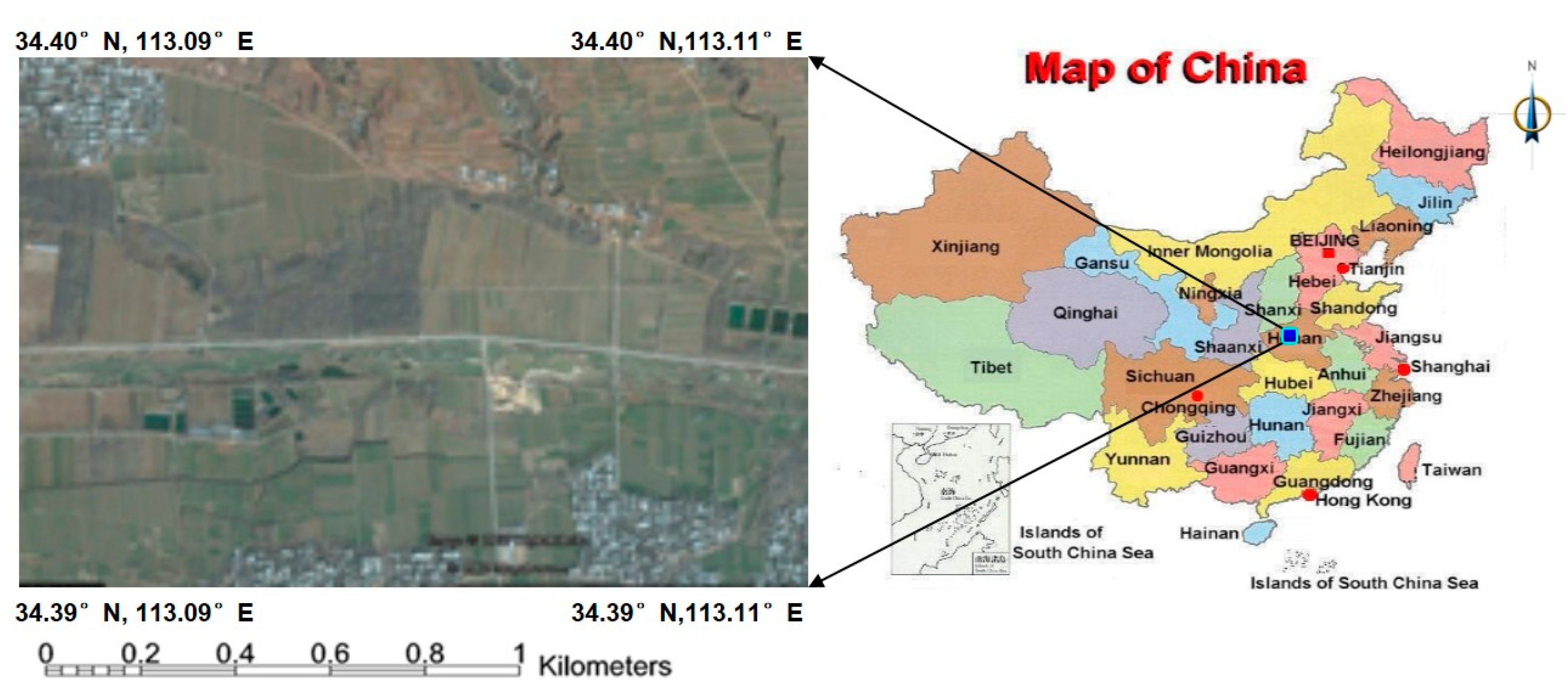
2.1. Study Area
2.2. CASMSAR Datasets

| Parameters | P-Band | X-Band |
|---|---|---|
| Acquired | 2011-06-23 | 2011-06-23 |
| Polarization | HH/HV/VH/VV | HH |
| Pixel size (m2) | 0.6 × 0.6 | 0.25 × 0.25 |
| Wavelength (m) | 0.5 | 0.03 |
| Spatial resolution (m) | 1 | 0.5 |
| Central frequency | 600 MHz | 9.6 GHz |
| Number of looks | 1 | 1 |
| Flight altitude (m) | 3155 | 3155 |
| Aircraft ground speed (m/s) | 115.5 | 115.5 |
| Incidence angle (°) | 43 | 50 |
| Incidence angle interval (°) | 10 | 13 |
| Slant range swath start (m) | 3496.31 | 2690.64 |
| Slant range swath end (m) | 12,097.91 | 12,418.64 |
2.3. Pre-Processing

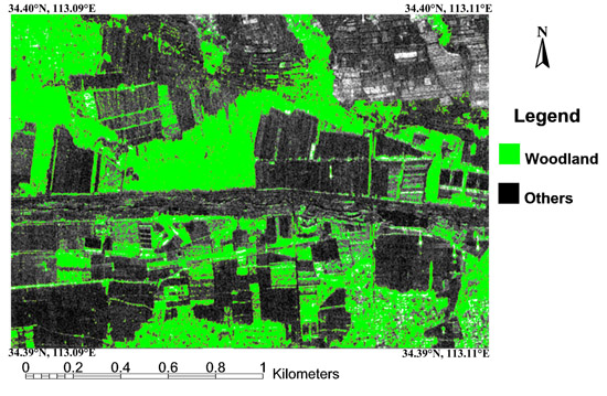
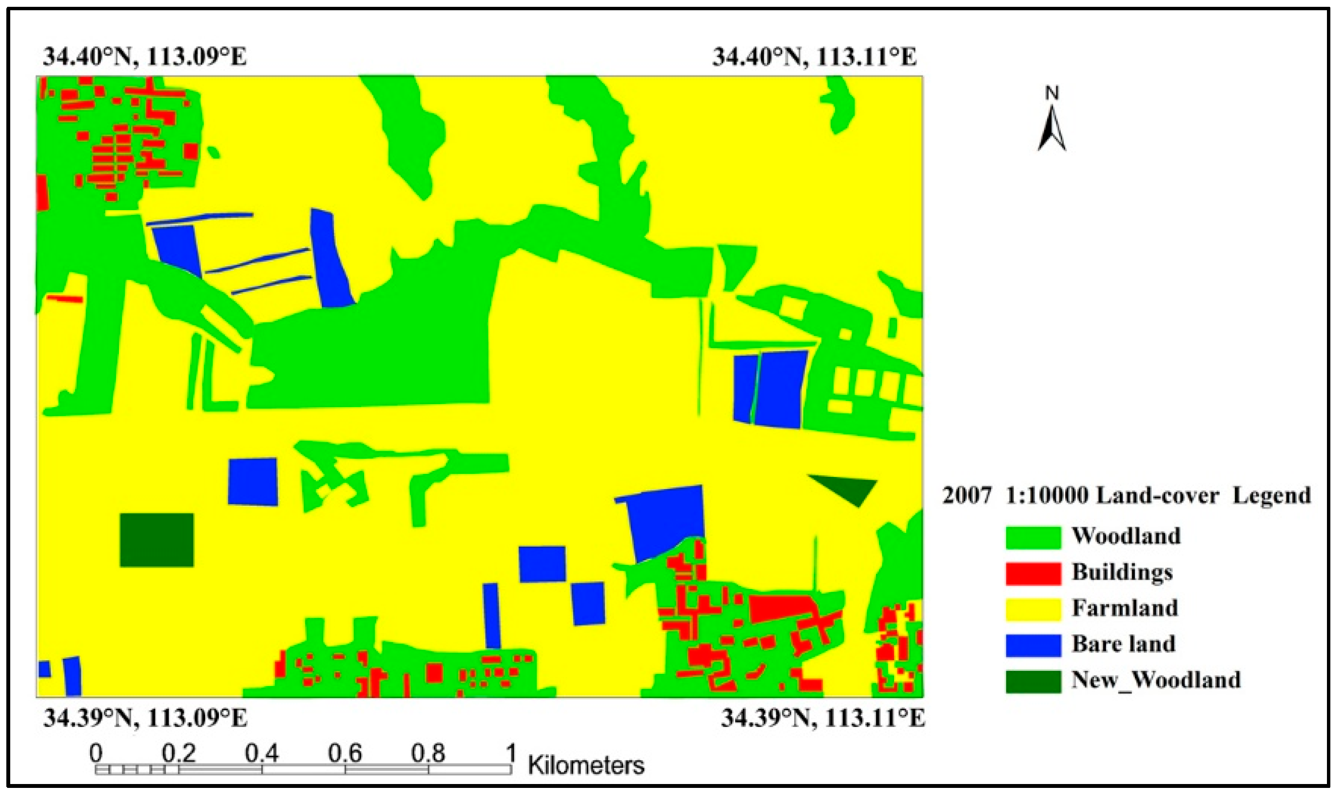
2.4. Land-Cover Data
3. Methods and Processing
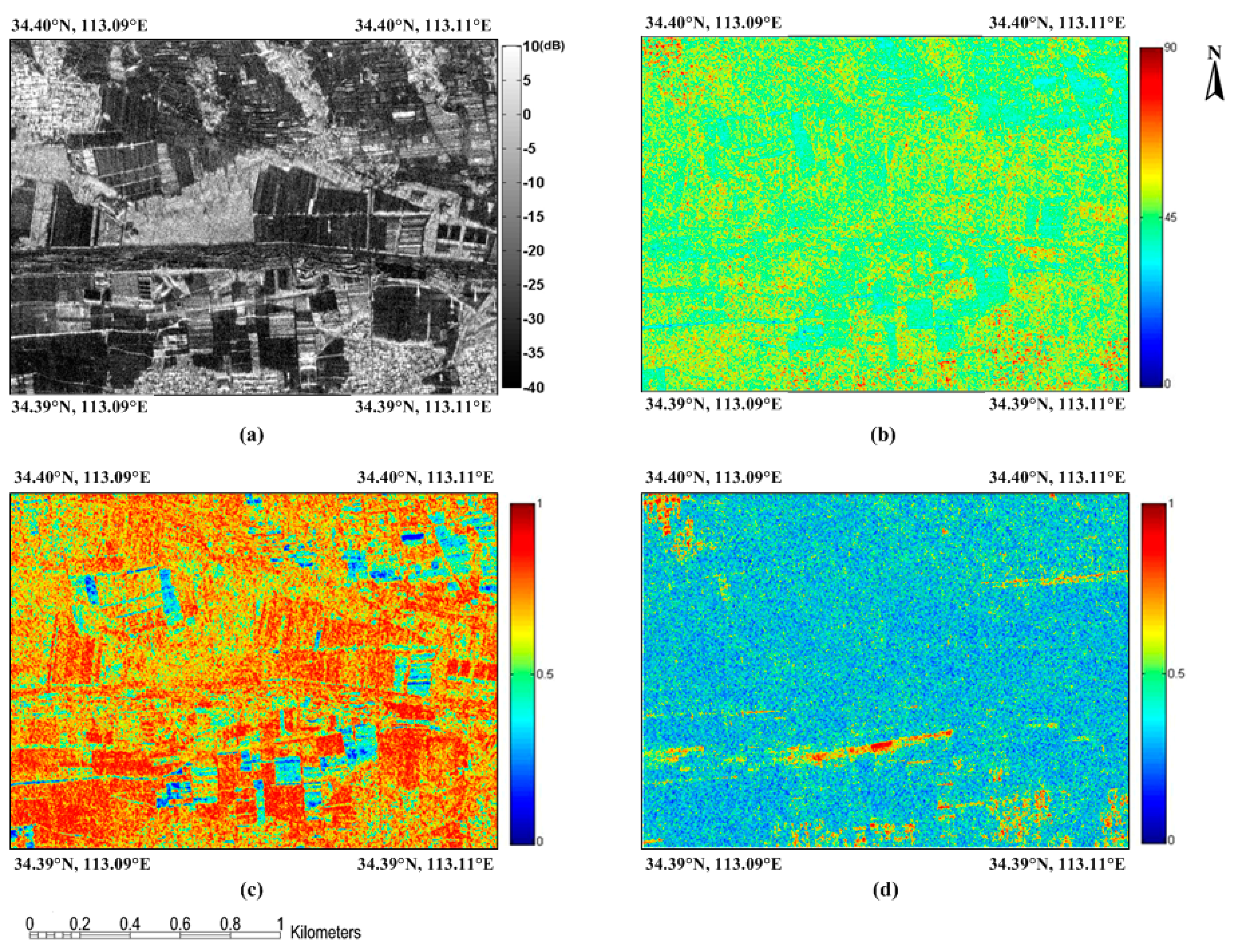
3.1. Single-Band SAR Data Processing
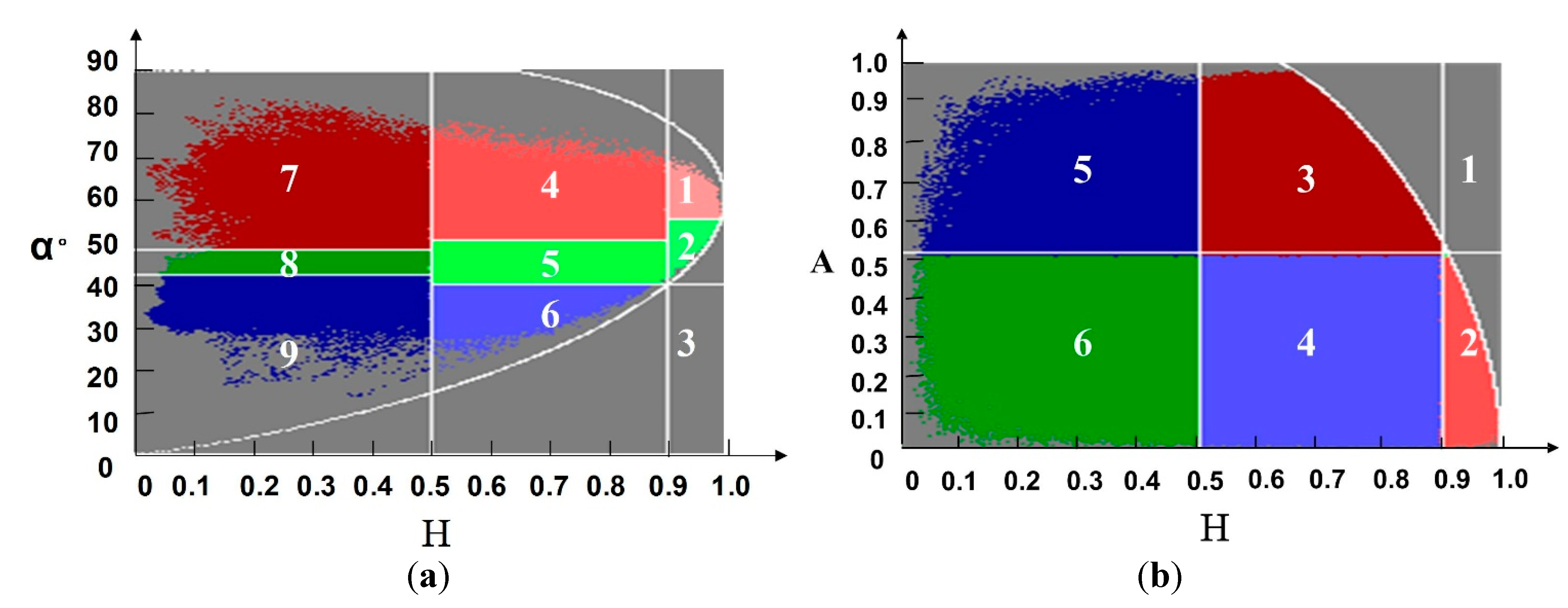
3.1.1. PolSAR Image Classification


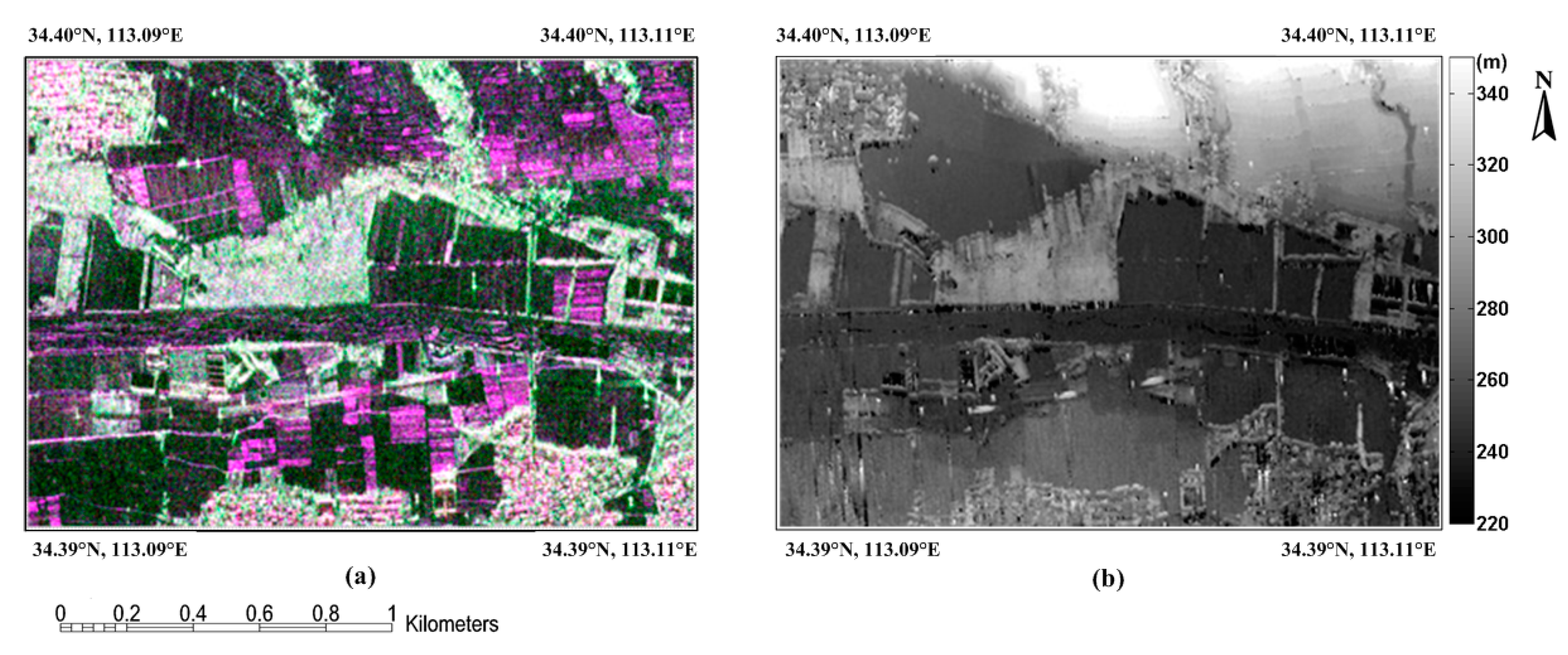
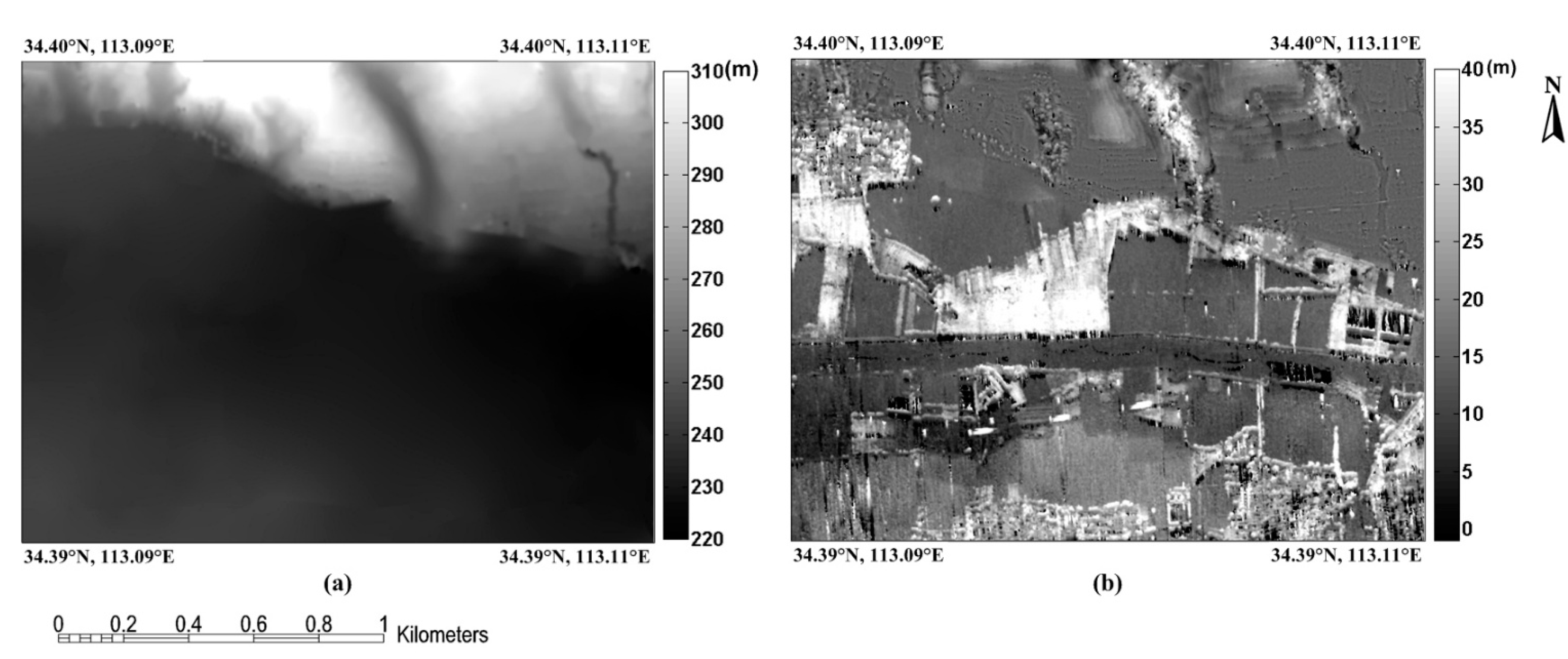
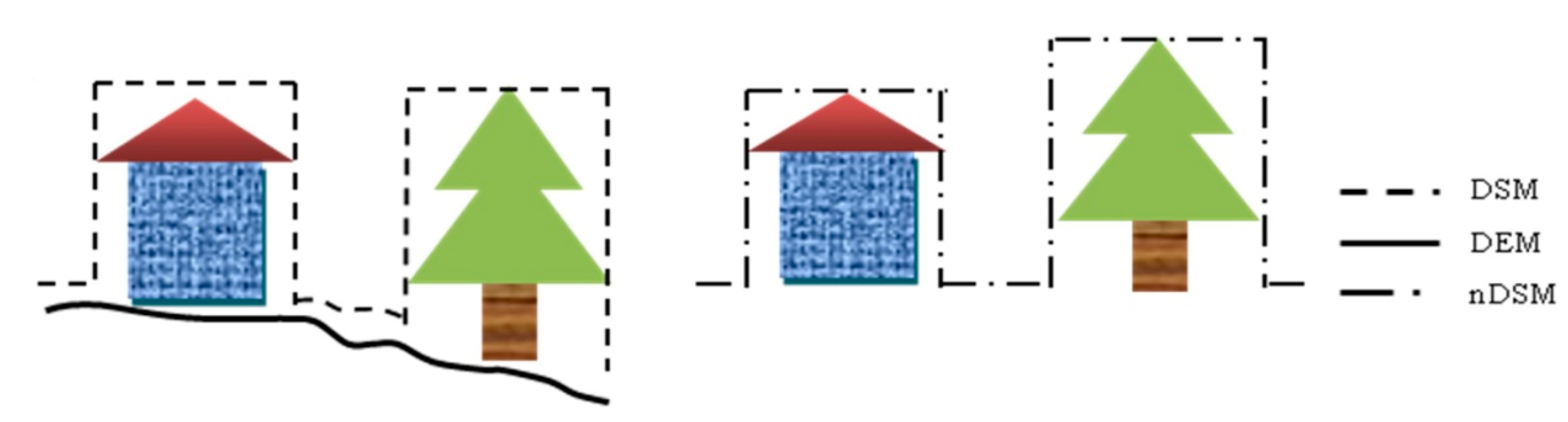
3.1.2. InSAR Elevation Map Classification


3.2. Dual-Band SAR Data Fusion Processing
3.2.1. High-Level Fusion Using Dempster-Shafer Evidence Theory
3.2.2. Combination and Decision
| Source | Woodland | Buildings | Farmland | Bareland |
|---|---|---|---|---|
| P-band data | =0.6 | =0.0 | =0.2 | =0.1 |
| X-band data | =0.2 | =0.0 | =0.3 | =0.2 |
| P-band | 0.6 | 0 | 0.2 | 0.1 | 0.1 | |
|---|---|---|---|---|---|---|
| 0.2 | Woodland 0.12 | 0 | 0.04 | 0.02 | Woodland 0.02 | |
| 0 | 0 | Buildings 0 | 0 | 0 | Buildings 0 | |
| 0.3 | 0.18 | 0 | Farmland 0.06 | 0.03 | Farmland 0.03 | |
| 0.2 | 0.12 | 0 | 0.04 | Bare land 0.02 | Bare land 0.02 | |
| 0.3 | Woodland 0.18 | Buildings 0 | Farmland 0.06 | Bare land 0.03 | C 0.03 | |
| = 0.32 = 0.00 = 0.15 = 0.07 = 0.03 | ||||||
| 1-K== 0.57 | ||||||
| 0.32/0.57 = 0.56 | 0.00/0.57 = 0.00 | 0.15/0.57 = 0.26 | 0.07/0.57 = 0.12 | |||
| Bel() | Bel() = 0.56 | Bel() = 0.00 | Bel() = 0.26 | Bel() = 0.12 | ||
| woodland, buildings, farmland, bare land. | ||||||
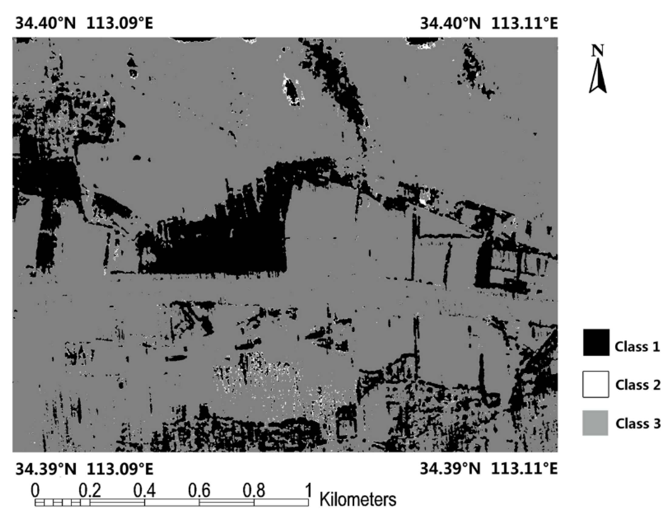
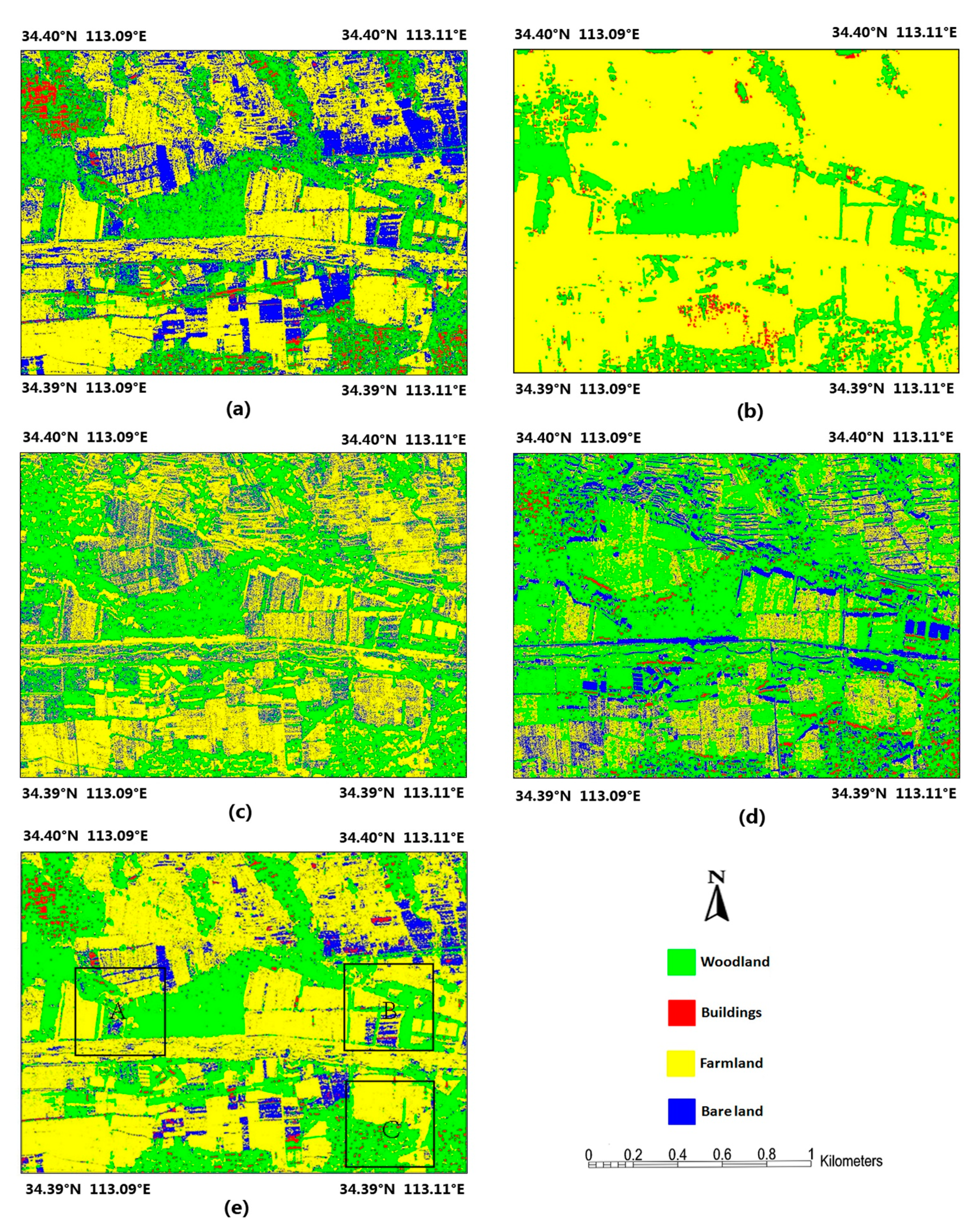
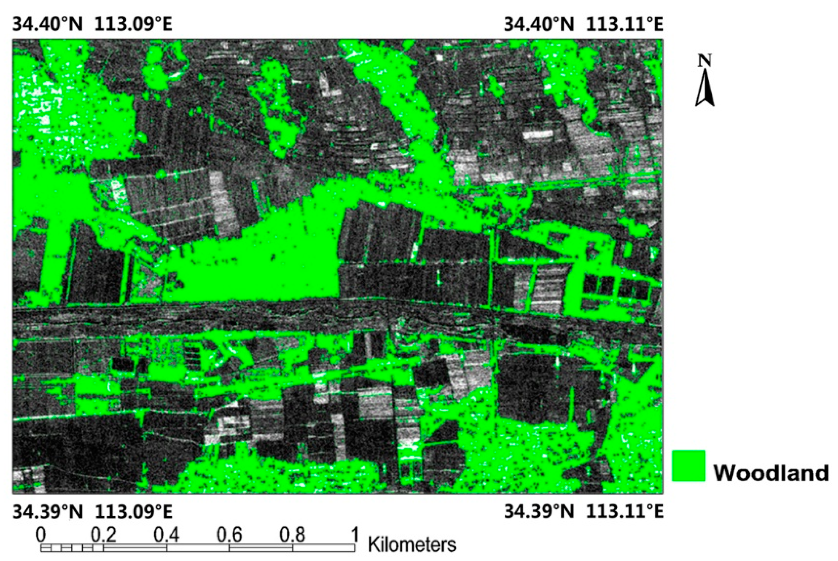
4. Results

| Land-Cover Class | Proportion(%) | Sample Number |
|---|---|---|
| Woodland | 31 | 258 |
| Buildings | 4 | 34 |
| Farmland | 56 | 465 |
| Bare land | 9 | 75 |
| Land-Cover Class | Ground Truth (%) | UA (%) | |||
|---|---|---|---|---|---|
| Woodland | Buildings | Farmland | Bareland | ||
| Woodland | 75.89 | 77.49 | 3.66 | 18.90 | 81.15 |
| Buildings | 0.00 | 6.55 | 0.01 | 0.00 | 98.00 |
| Farmland | 18.16 | 13.36 | 83.22 | 43.82 | 76.00 |
| Bare land | 5.96 | 2.61 | 13.11 | 37.28 | 34.05 |
| OA = 72.43% , Kappa = 0.55, Z = 3.43 | |||||
| Land-Cover Class | Ground Truth (%) | UA (%) | |||
|---|---|---|---|---|---|
| Woodland | Buildings | Farmland | Bareland | ||
| Woodland | 84.07 | 8.29 | 1.98 | 6.57 | 94.26 |
| Buildings | 4.60 | 89.32 | 0.27 | 0.13 | 61.11 |
| Farmland | 1.45 | 0.00 | 90.28 | 1.87 | 98.02 |
| Bare land | 9.88 | 2.39 | 7.48 | 91.42 | 61.75 |
| OA = 87.95%, Kappa = 0.82, Z = 1.90 | |||||
| Land-Cover Class | Ground Truth (%) | UA (%) | ||
|---|---|---|---|---|
| Woodland | Buildings | Farmland | ||
| Woodland | 92.41 | 26.39 | 4.36 | 92.12 |
| Buildings | 0.69 | 5.14 | 1.25 | 17.11 |
| Farmland | 6.83 | 68.34 | 94.36 | 90.11 |
| OA = 90.08%, Kappa = 0.80 | ||||
| Land-Cover Class | Ground Truth (%) | UA (%) | |||
|---|---|---|---|---|---|
| Woodland | Buildings | Farmland | Bareland | ||
| Woodland | 95.06 | 9.23 | 1.97 | 5.17 | 95.26 |
| Buildings | 3.74 | 88.38 | 5.64 | 0.00 | 43.17 |
| Farmland | 0.17 | 0.00 | 82.98 | 0.72 | 99.57 |
| Bare land | 1.03 | 2.39 | 9.41 | 94.11 | 72.15 |
| OA = 89.84%, Kappa = 0.84, Z = 1.88 | |||||
| Land-Cover Class | Ground Truth (%) | UA (%) | |||
|---|---|---|---|---|---|
| Woodland | Buildings | Farmland | Bareland | ||
| Woodland | 96.14 | 9.89 | 2.44 | 0.06 | 96.01 |
| Buildings | 0.02 | 90.05 | 0.08 | 2.88 | 88.92 |
| Farmland | 2.19 | 0.00 | 94.82 | 5.42 | 96.85 |
| Bare land | 1.61 | 0.00 | 2.41 | 91.62 | 86.11 |
| OA = 94.77%, Kappa = 0.92, Z = 1.80 | |||||
| Land-Cover Class | Modality | Selected Feature | Classification Accuracy (%) | Distinguishing Capability |
|---|---|---|---|---|
| Woodland | a | H, α, A | 84.07 | Medium |
| b | elevation | 92.41 | High | |
| c | H, α, A, elevation | 96.14 | High | |
| Buildings | a | H, α, A | 89.32 | Medium |
| b | elevation | 5.14 | low | |
| c | H, α, A, elevation | 90.05 | High | |
| Farmland | a | span | 90.28 | High |
| b | elevation | 94.36 | High | |
| c | span, elevation | 94.82 | High | |
| Bare land | a | H, α | 91.42 | High |
| b | × | × | × | |
| c | H, α | 91.62 | High |

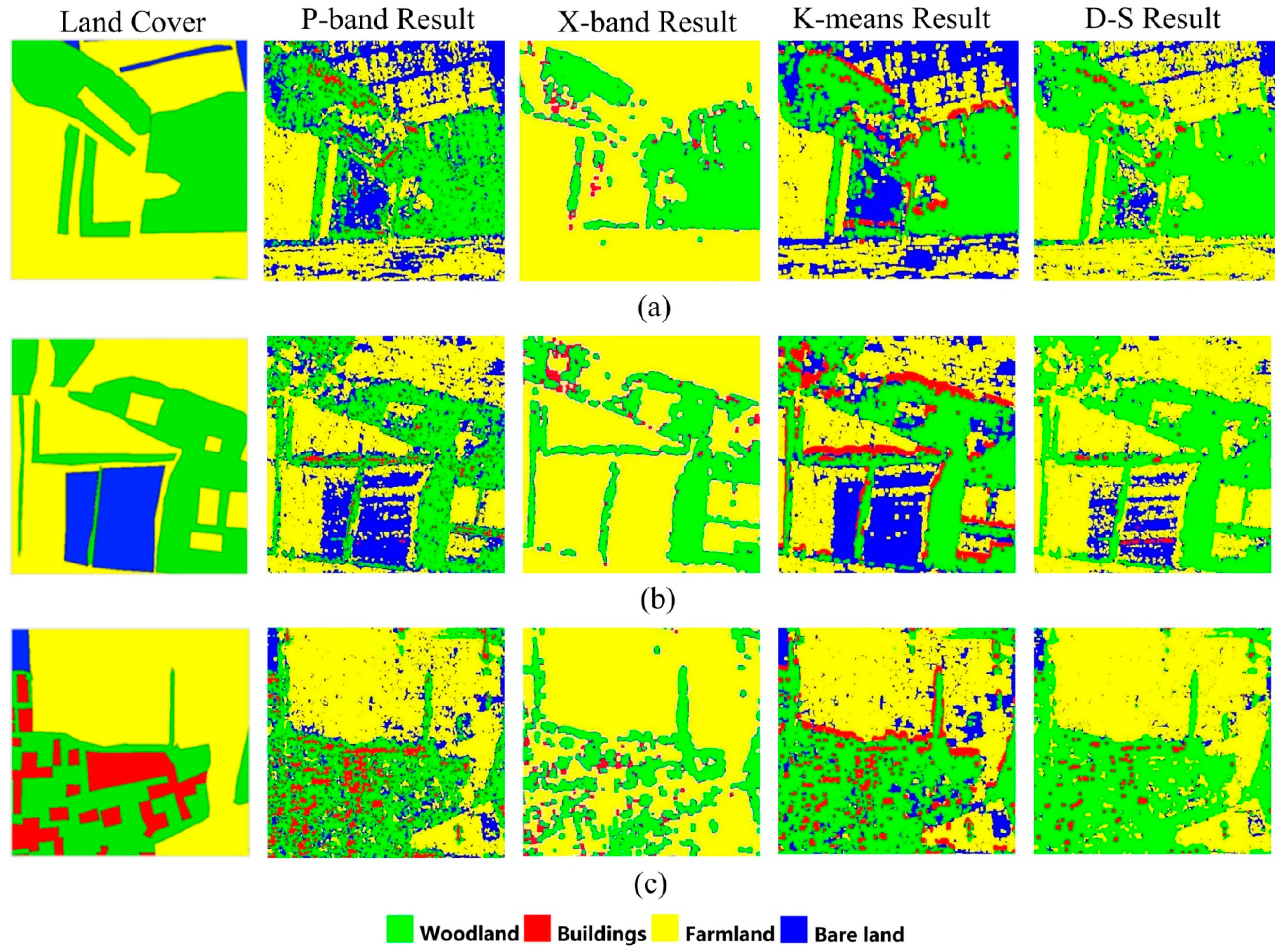
5. Discussion

| Woodland Extraction Methods | Region Umber | PA (%) | UA (%) | Z |
|---|---|---|---|---|
| P-band supervised classification | A | 85.78 | 93.69 | 2.80 |
| B | 84.54 | 94.98 | 2.51 | |
| C | 83.68 | 75.89 | 2.92 | |
| X-band unsupervised classification | A | 94.83 | 95.62 | 1.87 |
| B | 93.51 | 81.09 | 2.65 | |
| C | 86.46 | 57.31 | 3.35 | |
| K-means fusion | A | 93.77 | 95.50 | 1.88 |
| B | 88.24 | 90.39 | 1.93 | |
| C | 86.16 | 70.74 | 3.02 | |
| D-S fusion | A | 93.52 | 94.00 | 1.95 |
| B | 89.93 | 96.23 | 1.89 | |
| C | 95.68 | 61.52 | 3.00 |
6. Conclusions
Acknowledgments
Author Contributions
Conflicts of Interest
References
- The Central People’s Government of People’s Republic of China. Available online: http://www.gov.cn/flfg/2005-09/27/content_70635.htm (accessed on 22 January 2014).
- Gibbs, H.K.; Brown, S.; Niles, J.O.; Foley, J.A. Monitoring and estimating tropical forest carbon stocks: Making REDD a reality. Environ. Res. Lett. 2007, 2, 1–13. [Google Scholar]
- Saatchi, S.S.; Rignot, E. Classification of boreal forest cover types using SAR images. Remote Sens. Environ. 1997, 60, 270–281. [Google Scholar] [CrossRef]
- Maghsoudi, Y.; Collins, M.J.; Leckie, D.G. Radarsat-2 Polarimetric SAR Data for boreal forest classification using SVM and a wrapper feature selector. IEEE J. Sel. Top. Appl. Earth Obs. Remote Sens. 2013, 6, 1531–1537. [Google Scholar] [CrossRef]
- Xiao, W.S.; Wang, X.Q.; Ling, F.L. The application of ALOS PALSAR data on mangrove forest extraction. IEEE J. Sel. Top. Appl. Earth Obs. Remote Sens. 2010, 25, 91–96. [Google Scholar]
- Wang, H.P.; Ouchi, K.; Jin, Y.Q. Extraction of typhoon-damaged forests from multi-temporal high-resolution polarimetric SAR images. In Proceedings of the IGARSS 2010 Symposium, Honolulu, HI, USA, 25–30 July 2010.
- Quegan, S.; Le; Toan, T.; Yu, J.J.; Ribbes, F.; Floury, N. Multitemporal ERS SAR analysis applied to forest mapping. IEEE Trans. Geosci. Remote Sens. 2000, 38, 741–753. [Google Scholar] [CrossRef]
- Rignot, E.J.M.; Williams, C.L.; Way, J.; Viereck, L.A. Mapping of forest types in Alaskan boreal forests using SAR imagery. IEEE Trans. Geosci. Remote Sens. 1994, 32, 1051–1059. [Google Scholar] [CrossRef]
- Knowlton, D.J.; Hoffer, R.M. Radar imagery for forest cover mapping. In Proceedings of the Machine Processing of Remotely Sensed Data Symposium, West Lafayette, IN, USA, 23–26 June 1981.
- Drieman, J.A.; Ahern, F.J.; Corns, I.G.W. Visual interpretation results of multipolarization C-SAR imagery of Alberta boreal forest. In Proceedings of IGARSS’89,the 12th Canadian Symposium on Remote Sensing, Vancouver, BC, Canada, 10–14 July 1989.
- Liesenberg, V.; Gloaguen, R. Evaluating SAR polarization modes at L-band for forest classification purposes in Eastern Amazon, Brazil. Int. J. Appl. Earth Obs. Geoinf. 2013, 21, 122–135. [Google Scholar] [CrossRef]
- Dobson, M.C.; Ulaby, F.T.; Letoan, T.; Beaudoin, A.; Kasischke, E.S.; Christensen, N. Dependence of radar backscatter on coniferous forest biomass. IEEE Trans. Geosci. Remote Sens. 1992, 30, 412–415. [Google Scholar] [CrossRef]
- Hirosawa, H.; Matsuzaka, Y.; Kobayashi, O. Measurement of microwave backscatter from a cypress with and without leaves. IEEE Trans. Geosci. Remote Sens. 1989, 27, 698–701. [Google Scholar] [CrossRef]
- Van der Sanden, J.J.; Hoekman, D.H. Potential of airborne radar to support the assessment of land cover in a tropical rain forest environment. Remote Sens. Environ. 1999, 68, 26–40. [Google Scholar] [CrossRef]
- Ulander, L.; Dammert, P.B.G.; Hagberg, J.O. Measuring tree height with ERS-1 SAR interferometry. In Proceedings of the IGARSS’95 Symposium, Florence, Italy, 10–14 July 1995.
- Takeuchi, S.; Oguro, Y. A comparative study of coherence patterns in C-band and L-band interferometric SAR from tropical rain forest areas. Adv. Space Res. 2003, 32, 2305–2310. [Google Scholar] [CrossRef]
- Wegmuller, U.; Werner, C.L. SAR interferometric signatures of forest. IEEE Trans. Geosci. Remote Sens. 1995, 33, 1153–1161. [Google Scholar] [CrossRef]
- Wegmiiller, U.; Werner, C.L. Retrieval of vegetation parameters with SAR interferometry. IEEE Trans. Geosci. Remote Sens. 1997, 35, 18–24. [Google Scholar] [CrossRef]
- Simard, M.; Saatchi, S.S.; de Grandi, G. The use of decision tree and multiscale texture for classification of JERS-1 SAR data over tropical forest. IEEE Trans. Geosci. Remote Sens. 2000, 38, 2310–2321. [Google Scholar] [CrossRef]
- Chen, C.T.; Chen, K.S.; Lee, J.S. The use of fully polarimetric information for the fuzzy neural classification of SAR images. IEEE Trans. Geosci. Remote Sens. 2003, 41, 2089–2100. [Google Scholar] [CrossRef]
- Waske, B.; Linden, S. Classifying multilevel imagery from SAR and optical sensors by decision fusion. IEEE Trans. Geosci. Remote Sens. 2008, 46, 1457–1466. [Google Scholar] [CrossRef]
- Seetharamana, K.; Palanivelb, N. Texture characterization, representation, description, and classification based on full range Gaussian Markov random field model with Bayesian approach. Int. J. Image Data Fusion 2013, 4, 342–362. [Google Scholar] [CrossRef]
- Berger, O.B. Statistical Decision Theory and Bayesian Analysis. Springer Series in Statistics; Springer-Verlag: New York, NY, USA, 1985. [Google Scholar]
- Shafer, G. A Mathematical Theory of Evidence; Princeton University Press: Princeton, NJ, USA, 1976. [Google Scholar]
- Dubois, D.; Prade, H.; Yager, R. Merging fuzzy information. In Handbook of Fuzzy Sets Series, Approximate Reasoning and Information Systems; Springer: Boston, MA, USA, 1999; pp. 335–401. [Google Scholar]
- Lein, J.K. Applying evidential reasoning methods to agricultural land cover classification. Int. J. Remote Sens. 2003, 24, 4161–4180. [Google Scholar] [CrossRef]
- Mascle, S.L.H.; Bloch, I.; Madjar, D.V. Application of Dempster-Shafer evidence theory to unsupervised classification in multisource remote sensing. IEEE Trans. Geosci. Remote Sens. 1997, 35, 1018–1031. [Google Scholar] [CrossRef]
- Cayuela, L.; Golicher, J.D.; Salas Rey, J.; Rey Benayas, J.M. Classification of a complex landscape using Dempster-Shafer theory of evidence. Int. J. Remote Sens. 2006, 27, 1951–1971. [Google Scholar] [CrossRef]
- Milisavljević, N.; Bloch, I.; Alberga, V.; Satalino, G. Three strategies for fusion of land cover classification results of polarimetric SAR data. In Sensor and Data Fusion; I-Tech: Vienna, Austria, 2009; pp. 277–298. [Google Scholar]
- Yang, M.S.; Moon, W.M. Decision level fusion of multi-frequency polarimetric SAR and optical data with Dempster-Shafer evidence theory. In Proceedings of the IGARSS’03 Symposium, Toulouse, France, 21–25 July 1993.
- Rodríguez-Cuenca, B.; Alonso, M.C. Semi-automatic detection of swimming pools from aerial high-resolution images and LiDAR data. Remote Sens. 2014, 6, 2628–2646. [Google Scholar] [CrossRef]
- Zhang, J.X.; Zhao, Z.; Huang, G.M.; Lu, Z. CASMSAR: An Integrated Airborne SAR Mapping system. Photogramm. Eng. Remote Sens. 2012, 78, 1110–1114. [Google Scholar]
- Lee, J.S.; Grunes, M.R.; Grandi, G. Polarimetric SAR speckle filtering and its implication for classification. IEEE Trans. Geosci. Remote Sens. 1999, 37, 2363–2373. [Google Scholar] [CrossRef]
- Lee, J.S.; Grunes, M.R.; Kwok, R. Classification of multi-look polarimetric SAR imagery based on the complex Wishart distribution. Int. J. Remote Sens. 1994, 15, 2299–2311. [Google Scholar] [CrossRef]
- Chan, C.Y. Studies on the Power Scattering Matrix of Radar Targets. Master’s Thesis, University of Illinois, Chicago, IL, USA, 1981. [Google Scholar]
- Cloude, S.R.; Pottier, E. Anentropy based classification scheme for land applications of polarimetric SAR. IEEE Trans. Geosci. Remote Sens. 1997, 35, 68–78. [Google Scholar] [CrossRef]
- Hajnsek, I.; Pottier, E.; Cloude, S.R. Inversion of surface parameters from polarimetric SAR. IEEE Trans. Geosci. Remote Sens. 2003, 41, 727–744. [Google Scholar] [CrossRef]
- Rowland, C.S.; Balzter, H. Data fusion for reconstruction of a DTM, under a woodland canopy, from airborne L-band InSAR. IEEE Trans. Geosci. Remote Sens. 2007, 45, 1154–1163. [Google Scholar] [CrossRef] [Green Version]
- Dash, J.; Steinle, E.; Singh, R.P.; Bähr, H.P. Automatic building extraction from laser scanning data: An input tool for disaster management. Adv. Space Res. 2004, 33, 317–322. [Google Scholar] [CrossRef]
- Zhang, J.; Duan, M.; Yan, Q.; Lin, X. Automatic vehicle extraction from airborne LiDAR data using an object-based point cloud analysis method. Remote Sens. 2014, 6, 8405–8423. [Google Scholar] [CrossRef]
- Ostu, N. A Threshold Selection Method from Gray-Level Histograms. Available online: http://159.226.251.229/videoplayer/otsu1979.pdf?ich_u_r_i=e503462fdc95647446b6e497574284e6&ich_s_t_a_r_t=0&ich_e_n_d=0&ich_k_e_y=1545038930750163512478&ich_t_y_p_e=1&ich_d_i_s_k_i_d=4&ich_u_n_i_t=1 (accessed on 17 September 2014).
- Jensen, J.R. Digital change detection. In Introductory Digital Image Processing: A Remote Sensing Perspective; Prentice-Hall: New Jersey, NJ, USA, 2004; pp. 467–494. [Google Scholar]
- Rosenfield, G.H.; Fitzpatrick-Lins, K. A coefficient of agreement as a measure of thematic classification accuracy. Photogramm. Eng. Remote Sens. 1986, 52, 223–227. [Google Scholar]
- Congalton, R.G.; Green, K. Assessing the Accuracy of Remotely Sensed Data: Principles and Practices; Lewis: Boca Raton, FL, USA, 1999. [Google Scholar]
- Loveland, J.L. Mathematical Justification of Introductory Hypothesis Tests and Development of Reference Materials. Available online: http://digitalcommons.usu.edu/gradreports/14/ (accessed on 17 September 2014).
- Huang, Z.D. Western land cover mapping investigation. Geomatics Technol. Equip. 2009, 11, 38–39. [Google Scholar]
- Zhao, L.L.; Yang, J.; Li, P.X.; Zhang, L.; Shi, L.; Lang, F. Damage assessment in urban areas using post-earthquake airborne PolSAR imagery. Int. J. Remote Sens. 2013, 34, 8952–8966. [Google Scholar] [CrossRef]
- Santoro, M.; Wegmüller, U.; Askne, J.I.H. Signatures of ERS-ENVISAT interferometric SAR coherence and phase of short vegetation: An analysis in the case of Maize fields. IEEE Trans. Geosci. Remote Sens. 2010, 48, 1702–1713. [Google Scholar] [CrossRef]
© 2015 by the authors; licensee MDPI, Basel, Switzerland. This article is an open access article distributed under the terms and conditions of the Creative Commons Attribution license (http://creativecommons.org/licenses/by/4.0/).
Share and Cite
Lu, L.; Xie, W.; Zhang, J.; Huang, G.; Li, Q.; Zhao, Z. Woodland Extraction from High-Resolution CASMSAR Data Based on Dempster-Shafer Evidence Theory Fusion. Remote Sens. 2015, 7, 4068-4091. https://doi.org/10.3390/rs70404068
Lu L, Xie W, Zhang J, Huang G, Li Q, Zhao Z. Woodland Extraction from High-Resolution CASMSAR Data Based on Dempster-Shafer Evidence Theory Fusion. Remote Sensing. 2015; 7(4):4068-4091. https://doi.org/10.3390/rs70404068
Chicago/Turabian StyleLu, Lijun, Wenjun Xie, Jixian Zhang, Guoman Huang, Qiwei Li, and Zheng Zhao. 2015. "Woodland Extraction from High-Resolution CASMSAR Data Based on Dempster-Shafer Evidence Theory Fusion" Remote Sensing 7, no. 4: 4068-4091. https://doi.org/10.3390/rs70404068