Article

Comparing MODIS Net Primary Production Estimates with Terrestrial National Forest Inventory Data in Austria

1
Institute of Silviculture, Department of Forest and Soil Sciences, University of Natural Resources and Life Sciences, Vienna, Peter-Jordan-Str. 82, A-1190 Vienna, Austria
2
Department of Geographical Sciences, University of Maryland, College Park, MD 20742, USA
3
Natural Hazards and Landscape, Department of Forest Growth and Silviculture, Federal Research and Training Centre for Forests, Vienna, Seckendorff-Gudent-Weg 8, A-1130 Vienna, Austria
*
Author to whom correspondence should be addressed.
Remote Sens. 2015, 7(4), 3878-3906; https://doi.org/10.3390/rs70403878
Submission received: 11 December 2014 / Revised: 12 March 2015 / Accepted: 17 March 2015 / Published: 1 April 2015

Abstract

:
The mission of this study is to compare Net Primary Productivity (NPP) estimates using (i) forest inventory data and (ii) spatio-temporally continuous MODIS (MODerate resolution Imaging Spectroradiometer) remote sensing data for Austria. While forest inventories assess the change in forest growth based on repeated individual tree measurements (DBH, height etc.), the MODIS NPP estimates are based on ecophysiological processes such as photosynthesis, respiration and carbon allocation. We obtained repeated national forest inventory data from Austria, calculated a “ground-based” NPP estimate and compared the results with “space-based” MODIS NPP estimates using different daily climate data. The MODIS NPP estimates using local Austrian climate data exhibited better compliance with the forest inventory driven NPP estimates than the MODIS NPP predictions using global climate data sets. Stand density plays a key role in addressing the differences between MODIS driven NPP estimates versus terrestrial driven inventory NPP estimates. After addressing stand density, both results are comparable across different scales. As forest management changes stand density, these findings suggest that management issues are important in understanding the observed discrepancies between MODIS and terrestrial NPP.

Graphical Abstract

1. Introduction

Productivity estimates are important measures to characterize the mass budget of a forest ecosystem. In this context, the carbon balance and carbon storage of the earth’s ecosystems and their spatial and temporal development is important. A measure for the carbon flux is Net Primary Production (NPP) which describes the carbon uptake by vegetation through photosynthesis. In principle, large scale carbon measures are currently provided by National Forest Inventories, flux towers and remotely sensed methods, such as the MODIS (MODerate resolution Imaging Spectroradiometer) NPP algorithm.
Researchers in previous studies have compared MODIS satellite-driven NPP with NPP estimates derived using terrestrial data [1,2,3]. Shvidenko et al. [1] found that for Russia the two estimates comply on average. Pan et al. [2] observed deviations between MODIS and terrestrial NPP using inventory data from the mid-Atlantic region of the USA and suggest that differences in water availability explain this variation. Hasenauer et al. [3] also found similar deviations and concluded that the different data sources for predicting NPP compare well after addressing forest management impacts. The authors further suggest that a combination of “ground-based” forest data with “space-based” forest productivity estimates would utilize the advantages of both methods.
National forest inventories are established for a continuous monitoring of the forest situation across countries. They are often based on a systematic permanent grid design. For each sample plot, a limited number of trees compared to the total forest area [4] is recorded to provide information on the standing growing stock, increment, species composition and other information needs relevant for forest management [5,6]. Such forest inventories are usually repeated every five to 10 years. Examples for national long term forest inventories can be found in countries such as Austria, Norway, Finland, Germany, etc. [4].
The MODIS NPP algorithm is based on remote sensing techniques and was developed for estimating large-scale forest productivity [7,8]. MODIS is a satellite-mounted sensor operated by the National Aeronautics and Space Administration of the United States (NASA) that provides large-scale information on global dynamics and processes. The MODIS algorithm MOD17 uses satellite data, climate data and biophysical properties of various cover types to derive eight-day GPP (Gross Primary Production) and NPP estimates on a 1 × 1 km pixel resolution. This data source may be seen as a “space-based” approach and provides continuous coverage across the global land area to assess forest productivity.
The differences of the two approaches are as follows:
(i)
The MODIS satellite-driven NPP is based on the principles of carbon uptake following light use efficiency logic [9] using a simplification of the NPP algorithms implemented in BIOME-BGC [10]. According to the hypothesis put forth by Hasenauer et al. [3] the MODIS NPP algorithm assumes a fully stocked forest for a given vegetation class or biome type and provides eight-day results NPP estimates on a 1 × 1 km grid.
(ii)
NPP estimates derived from terrestrial forest growth data (permanent sampling plots or forest inventory data) employ biomass expansion factors or biomass functions based on repeated observations such as breast height diameter (dbh) and/or tree height (h). Depending on the measurement interval the derived increment results represent a mean periodic average. Since this method is based on individual tree observations (e.g., dbh, h), potential changes in tree growth due to stand age, stand density or environmental effects such as weather patterns or CO2 concentration are included as they affect dbh and h development.
Several studies have compared satellite to terrestrial inventory data [1,2,11,12,13,14,15,16], however, no analysis has compared forest inventory data to MODIS NPP in Central Europe.
The mission of this paper is to compare space-based MODIS satellite-driven NPP data to ground-based inventory data driven NPP estimates using the Austrian National Forest Inventory Data. This Forest Inventory is based on a systematic permanent grid design with repeated observations [5,17]. The objectives of our study are:
(i)
obtain MODIS NPP estimates (using different climate data) for comparing the results with terrestrial-driven NPP estimates
(ii)
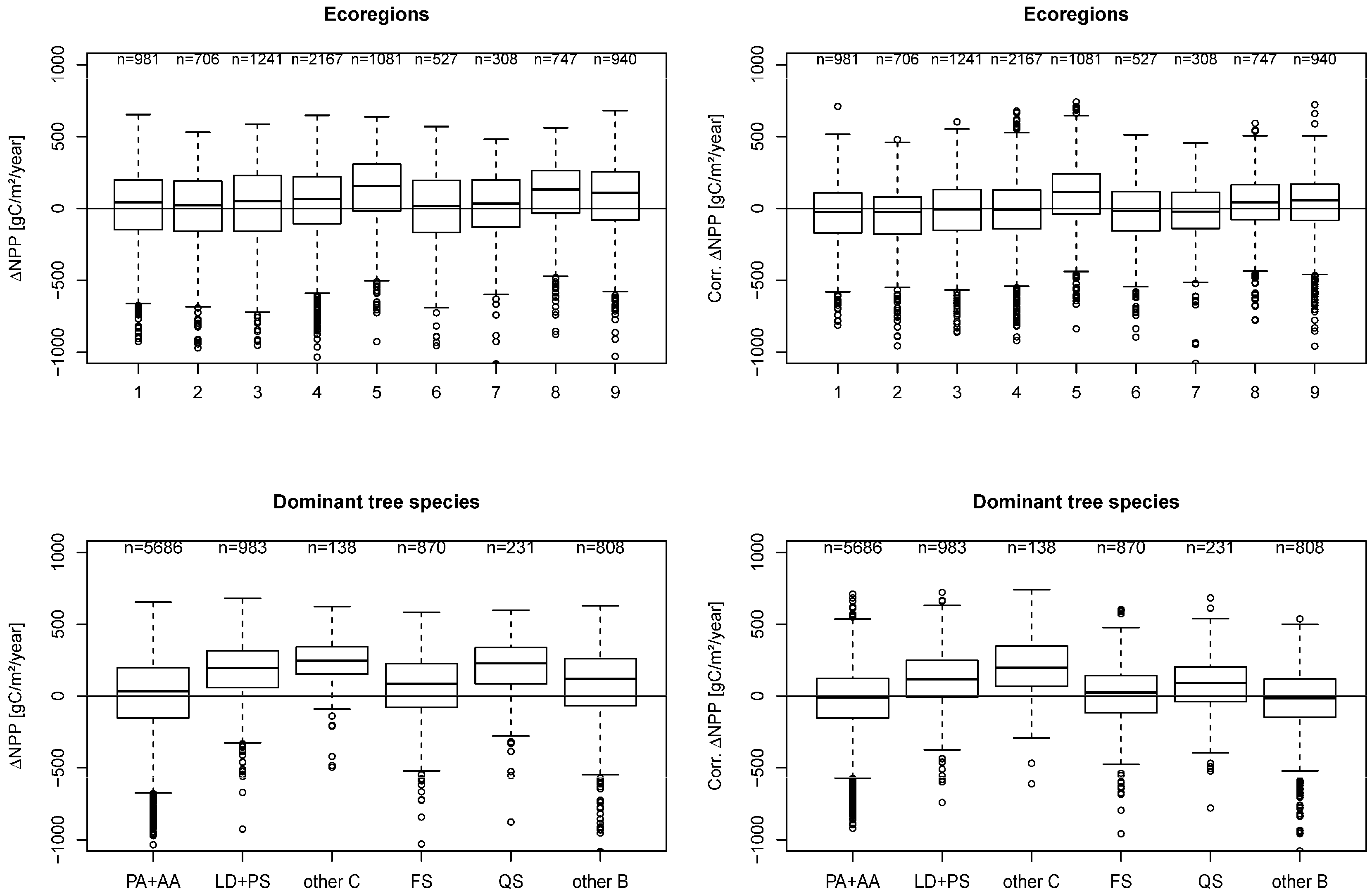
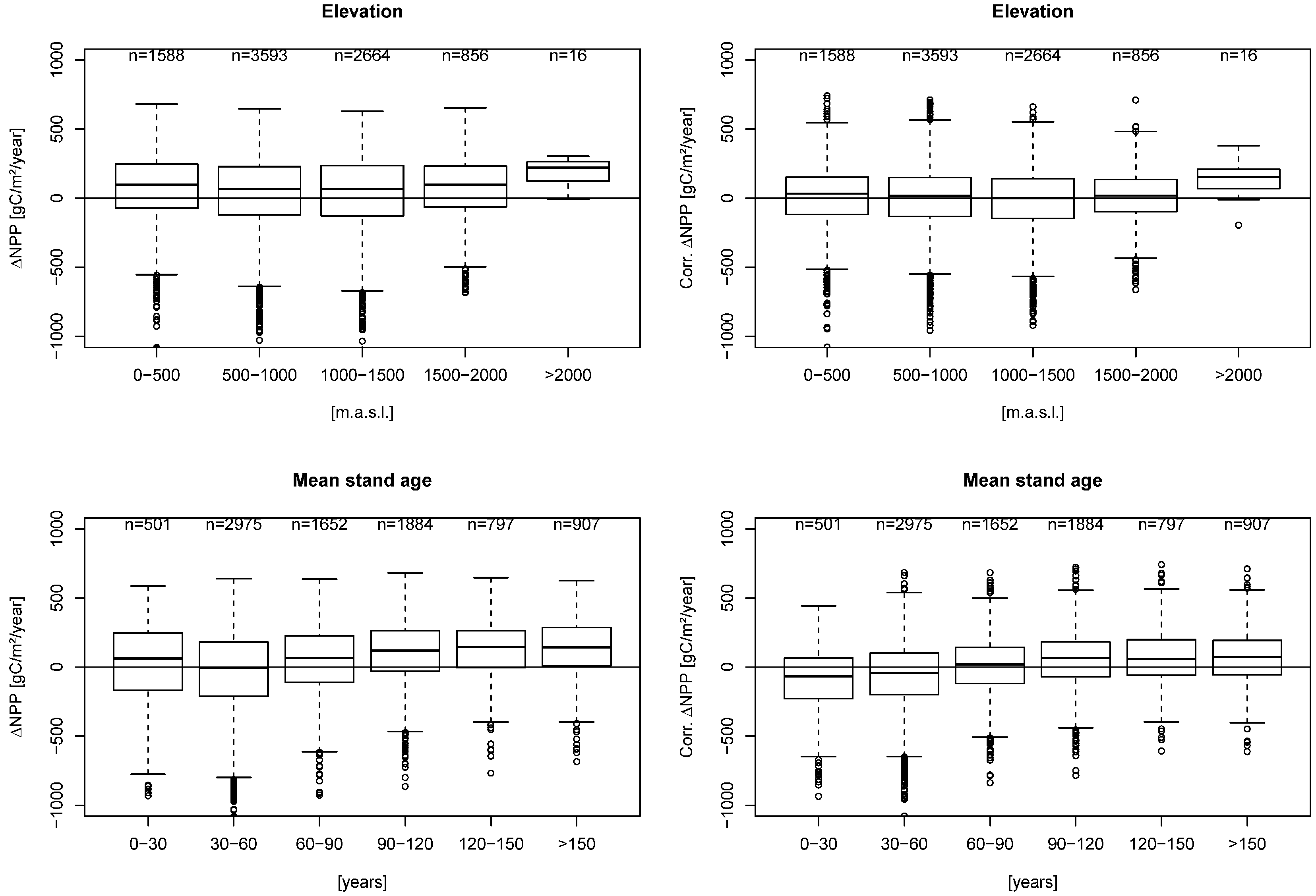
examine the potential effects of stand density, MODIS land cover types, stand age, species composition, ecoregion and elevation on NPP estimates by method.

2. Methods

2.1. MODIS NPP—“Space Based” Approach

We use the algorithms for the MODIS products MOD17A2 and MOD17A3, which provide global Gross and Net Primary Production (GPP, NPP) estimates for a 1 × 1 km pixel on an eight-day time-step [7,8]. The algorithm calculates GPP as
G P P = L U E max × 0.45 × S W r a d × F P A R × f V P D × f T m i n
where LUEmax is the maximum light use efficiency, SWrad is the short wave solar radiation load at the surface of which 45% is photosynthetically active, FPAR the fraction of absorbed PAR (Photosynthetic Active Radiation) from the MOD15 product, and fVPD and fTmin, which are multipliers between 0 and 1 addressing water stress due to vapor pressure deficit (VPD) and low temperature limits (Tmin, daily minimum temperature). Values that determine the LUEmax and the Tmin and VPD multipliers limits are stored in the Biome Property Type Look Up Tables (BPLUT) and cover five forest biome types: (i) ENF—Evergreen Needleleaf Forest, EBF—Evergreen Broadleaf Forest, DNF—Deciduous Needleleaf forest, DBF—Deciduous Broadleaf Forest, and MF—Mixed Forests ([3] for the model coefficients).
Annual Net Primary Production (NPP) is calculated from Gross Primary Production (GPP) by subtracting the autotrophic respiration components (i) maintenance respiration Rm and (ii) growth respiration Rg and summing up over a year to get annual values:
N P P = i = 1 365 G P P R m R g
With 366 days for leap years, Rm and Rg are calculated using leaf area index (LAI) from the MOD15 product, climate data, and parameters from the BPLUTs. For further details, please refer to the original literature [7,8].

2.2. Terrestrial NPP—“Ground Based” Approach

NPP can be calculated as the sum of biomass increment, mortality, and turnover of foliage and fine roots [18]. We employ volume and biomass functions along with repeated observations to get increment and mortality. Turnover of foliage, including mortality of other plant components, is represented by a climate-sensitive litterfall model [19]. The advantage of this model is the requirement of little input data and assumptions compared to calculating litterfall using biomass and turnover rates [18]. We lack a reliable model for fine root turnover in Austria and we assume that carbon uptake of fine roots is already incorporated in litterfall and coarse root increment.

2.2.1. Increment Estimation

Originally forest growth data was intended to provide volume increment in m3/ha per growth period [6]. The growth period varies depending on the temporal measurement interval of terrestrial sample plots. We develop a consistent and comparable terrestrial productivity data set by deriving NPP estimates using forest inventory data starting with:
N P P = i n c p l o t + C L i t t e r
where CLitter is the flow of dry carbon into litter [gC/m2/year] as defined in Equation (9), incplot is the dry carbon increment of trees (above and below ground biomass) [gC/m2/year] resulting from repeated plot observations taken at the end CForest_2 minus those observations taken at the beginning CForest_1 of the growth period
i n c p l o t = C F o r e s t _ 2 C F o r e s t _ 1
Equation (4) gives the common way to calculate increment for repeated observations and terrestrial plot data, the carbon values (CForest_1 and CForest_2) being the sum of the tree carbon estimates calculated from repeatedly measured diameters at breast height (dbh) and tree heights (h) for a given tree. The National Forest Inventory of Austria use a combined recording system with (i) fixed area plots for trees ranging in dbh from 5 cm to 10.4 cm and (ii) an angle count sampling system [20] for all trees with a dbh>10.4 cm. In angle count sampling the stem number represented by a sample tree changes by diameter and thus the represented tree population changes too, which differs from fixed-area plots (e.g., used in the National Forest Inventory system of Norway [4] or permanent research plots like the “Austrian Waldboden-Zustandsinventur” [21]). This affects volume or biomass stocks as well as periodic increment and thus the results from fixed area plot sampling are quite different compared to angle count sampling [6].
In principle, three different approaches in estimating increment form angle count sample data exist: (i) the starting value method; (ii) the end value method and (iii) the difference method.
For details we refer to Schieler [22] and Hasenauer and Eastaugh [6]. All three methods are statistically sound and deliver unbiased results [23,24].
For our study, we use the starting value method, which is also used by the Austrian National Forest Inventory:
i n c p l o t = Σ i n c s u r v i v o r s + Σ i n c i n g r o w t h
where incplot is the periodic increment on each plot resulting from ∑incsurvivors the “survivor trees”, which were also sampled in the last measurement, and ∑incingrowth the “ingrowth trees” or trees, which have reached the threshold during the re-measurement period and are thus selected [6,22,25]. The carbon increments of the “survivor trees“ are calculated as
Σ i n c s u r v i v o r s = Σ ( ( C 2 C 1 ) × n r e p 1 )
and the carbon increments of the “ingrowth trees” are
Σ i n c i n g r o w t h = Σ ( C 2 × n r e p 2 )
nrepi is the “represented” stem number per hectare at time 1 or time 2 and depends on the basal area factor k and the individual tree basal area g (for trees with dbh >10.4 cm nrepi = k/g and for trees with dbh 5–10.4 cm nrepi = 10,000/(2.62π) = 470.9). Ci are the carbon estimates for this “representative” tree at time 1 or time 2.

2.2.2. Carbon Estimation

The carbon increment calculation requires carbon estimates for each tree on a given inventory plot. For our study, we use the same method as applied by the Institute of Forest Inventory, Federal Research Centre for Forest, the agency responsible for the National Forest Inventory in Austria. The total dry carbon tree estimates of a single tree, Ci, can be calculated as follows:
C i = C C × ( d s m + d b m + d f m + d r m )
where CC is the carbon content and considered to be 0.5 for all species [26], dsm is the dry stem mass including bark, dbm the dry branch mass, dfm the dry foliage mass and drm the dry root mass with a diameter >2 mm.
The calculation of tree biomass is done using volume and biomass functions developed and used in Austria (see Appendix).

2.2.3. Litterfall Estimation

The last compartment for estimating NPP from terrestrial data in Equation (3) is the carbon flow into litter (CLitter). We select the method proposed by Liu et al. [19], which calculates the forest litter fall including all aboveground plant compartments according to Equations (9) and (10):
C L i t t e r = C C × L F
ln ( L F ) = 2.296 + 0.741 × ln ( T + 10 ) + 0.214 × ln ( P )
CLitter is the carbon in litterfall [gC/m2/year], CC carbon content equal 0.5 [26], LF total litter fall [g∙dry∙biomass/m2/year], T the mean annual temperature 2000–2010 [°C], P mean annual precipitation 2000–2010 [mm].

2.2.4. Stand Density Calculation

Forest management reduces stand density, stand density affects individual tree growth and thus the “ground-based” terrestrial NPP predictions [3]. For characterizing the stand density variation on the inventory plots we select the following two commonly used competition measures: CCF the crown competition factor [27] with Equation (11) and SDI the stand density index [28] with Equation (14):
C C F = P C A i × n r e p i A × 100 %
Where PCAi the species-specific potential crown area [m2] according to Equations (12) and (13)
P C A i = ( C W i 2 ) 2 × π
C W i = e c 0 + c 1 × ln ( d b h )
with nrepi as the representative stem number [ha−1] and A the observed area. CWi is the potential crown width [m] and dbh the diameter at breast height [cm]. The PCAi defines the crown area of a tree assuming open-grown conditions (the tree never experienced competition). Coefficients c0 and c1 in Equation (13) are derived from open-grown tree dimensions [29] and are given in Table A6 in the Appendix.
The Stand Density Index (SDI) is calculated according to Reinecke [28]:
S D I = N ( d g 25 ) 1.605
where N is the number of trees per unit area [ha−1], dg is the quadratic mean stand diameter at breast height [cm], 25 is a reference dg and 1.605 is the slope parameter for the maximum carrying capacity. The SDI has been proven to be site and age independent and SDImax defines an estimate for the carrying capacity of a given forest type [30].

2.2.5. Determining the Dominant Tree Species and the Ecoregions

One important aspect of our study is to assess potential effects of tree species on the MODIS and the NFI-driven productivity estimates. A grouping of the dominant tree species is done according to the main relative proportion of the basal area at a given inventory plot. The Norway Spruce (Picea abies (L.) Karst) and the Silver Fir (Abies alba Mill.), as relatively shade-tolerant species, are combined in one group. The Scots Pine (Pinus sylvestris (L.) Karst.) and the European Larch (Larix decidua Mill.) are light-demanding pioneer species and are also combined in one group. The two main broadleaf species groups are the Common Beech (Fagus sylvatica (L.)) and the Oak (Quercus spp.). These four groups cover 89% of the inventory plots. The remaining 11% are dominated by tree species which are aggregated into two groups: other coniferous trees and other broadleaf trees.
Austria has some very distinct biogeographic growth conditions due to the east-west aligned Alps. According to Kilian et al. [31], these differences lead to typical ecoregions (see Figure 1) and are characterized by similar environmental, macro-climatic as well as geological conditions leading to differences in potential vegetation. To assess the potential effect of these drivers, we assign the ecoregions to each inventory plot according to the plot location as outlined in Figure 1. With the ecoregions, we then can also examine the effect of geographical location on the results.

3. Data

3.1. Climate Data

Climate data is required as input to the MOD17 algorithms that derive MODIS NPP and for estimating the carbon content in the litterfall with Equations (9) and (10). Daily records of minimum and maximum temperature, precipitation, vapor pressure deficit and incident short wave radiation are interpolated from weather station data using DAYMET, a climate interpolation model [10] adapted and validated for Austrian conditions [32,33]. DAYMET interpolates daily precipitation and minimum and maximum temperatures from surrounding permanent climate stations. Based on the resulting climate data, daily solar radiation and vapor pressure data are calculated [34]. The current version of DAYMET [35] requires longitude, latitude, elevation, slope, aspect and the horizon angle facing east and west for each given plot. The meteorological data for running DAYMET were provided by the Austrian National Weather Center (ZAMG) in Vienna and include daily weather records from 250 stations across Austria since 1961. For our analysis, we generate daily weather data at a 1 × 1 km grid across the country.
For the MODIS NPP calculations we also use two additional climate data sets called “GMAO” and “NCEP2”, which are described in the next chapter.

3.2. MODIS Data

The storage system of MODIS data consists of 286 vegetated land tiles covering the whole globe. Each tile covers an area of 1200 × 1200 km or 1.44 million pixels. The MOD17 algorithm provides an eight-day GPP/NPP estimate for each 1 × 1 km pixel. We sum eight-day values to annual. We use the MODIS NPP product developed by Zhao et al. [36].
Previous studies showed that the direct use of 1 × 1 km MODIS pixel for validation may be inappropriate [37,38,39]. Reported reasons are (i) mismatch between MODIS gridded pixels and observations caused by gridding artifacts [38]; (ii) problems in the mixed land cover and surface reflectance information and (iii) uncertainties in the information provided for building the look-up tables [38]. We follow previous studies [3,37,38,39] and obtain the mean MODIS NPP of a 3 × 3 pixel patch (nine 1 x 1 km pixels) for each inventory plot. Within these 9 pixels we select only forest pixels according to the MOD12Q1 product [8] and the classification system of Friedl et al. [40]. Pixels with any other land cover type are ignored. For each of the forest pixels, we take the mean value of the MODIS NPP estimates according to three different climate input data sets provided by:
(1)
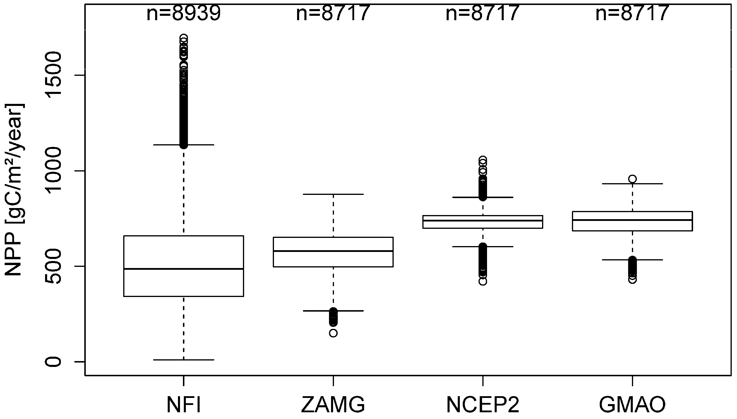
the NASA Global Modeling and Assimilation Offices (GMAO) at NASA Goddard Space Flight Center with a spatial resolution of 0.5 × 0.67° [41]. MODIS NPP derived from this data set will be referred to as “GMAO”.
(2)
the daily climate data set called NCEP_DOE_II with a spatial resolution of approx. 1.875 × 1.875° [42,43], referred to as “NCEP2”.
(3)
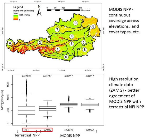
Austrian local daily climate data interpolated with DAYMET (see previous chapter) on 1 × 1 km (approx. 0.0083 × 0.0083°) resolution with station data provided by the Austrian National Weather Centre: “ZAMG”.
The difference between the MODIS NPP driven by GMAO and NCEP2 is caused by the different global daily climatology drivers and correspondingly modified BPLUT file [44]. The first two data sets are maintained by the Numerical Terra Dynamic Simulation Group (NTSG) at the University of Montana, while the Austrian local climate data are maintained by the Institute of Silviculture at The University of Natural Resources and Life Science, Vienna (BOKU).
From 1 January 2000 to 31 December 2011 for 11 full years all three variants of MODIS NPP estimates are computed. Until February 2000, missing MODIS data is considered negligible. Although the data is available annually, we use the periodic mean annual NPP for these 11 years to have a consistent and comparable temporal scaling with the forest inventory data. The variation between annual and periodic mean MODIS NPP is small (mean standard deviation 37.1 gC/m2/year) and shows no trend across Austria. The lack of trend and the low variation supports the use of the temporal aggregation.
Figure 1 gives the periodic mean annual MODIS driven NPP (2000–2011) estimates across the country and demonstrates the special feature of a “space-based” satellite-driven approach, providing continuous cover in productivity estimates for every km2 across Austria.
Figure 1. MODIS NPP for Austria calculated with NCEP2-climate data, black lines delineate forest ecoregions [31] used in the analysis.
Remotesensing 07 03878 g001

3.3. Forest Inventory Data

The National Austrian Forest Inventory is based on a systematic permanent grid design of 3.889 × 3.889 km over Austria with a cluster of four inventory plots at each grid point (approx. 22,000 plots and 5500 clusters). One cluster is a square with 200 m length on each side and a plot in each corner. The permanent plots were established during 1981–1985, where each year every 5th cluster was established. The inventory uses a hidden plot design where the center of each plot is marked with a hidden iron stick to eliminate research plot bias [45]. This is important because this procedure ensures that the Forest Inventory is representative for the growing conditions and forest management throughout Austria. The condition of the forest is measured on each plot with an angle count sample plot [20] using a basal area factor of 4 m2/ha for trees with dbh ≥10.4 cm and with a fixed area plot (r = 2.6 m, A = 21.2 m2) for trees with dbh ranging from 5.0 to 10.4 cm.
For details on the plot and sampling design, see Schadauer et al. [5] and Gabler and Schadauer [17]. For details on the applied sample methodology and its advantages and constraints, see literature [6,20,22,24,46].
We obtain the two most recent inventory measurements for our study: NFI 6, plot data recorded from 2000 to 2002, and NFI 7, plot data recorded from 2007 to 2009 resulting in a re-measurement interval of seven years [17]. We calculate periodic mean annual increment incplot with Equations (3)–(5).
Measurements of diameter at breast height (1.3 m) were taken for all sample trees. In NFI 6, tree height and height to the live crown base were only recorded for a subsample of trees on each plot. The missing estimates were estimated by applying dbh-dependent models. In NFI 7, tree height, height to the live crown base and dbh were recorded for every tree [17]. Data are available for approximately 9000 plots. Table 1 shows the summary statistics of the data available from the inventory plots for our analysis.

4. Results and Analysis

For the presented results and figures, the median is used which is less affected by outliers and skewed distributions. In the text the arithmetic mean is given, however, any comparison based on mean values assumes a symmetric distribution of the results and a balanced age class distribution of forests.

4.1. MODIS NPP versus Terrestrial NPP

Since three different daily climate data sets are available for deriving MODIS NPP across Austria, we explore the impact of different daily climate data on the resulting MODIS NPP computations. We compute the MOD17 NPP estimates for the years 2000–2011 using three different daily climate data sets: (i) GMAO; (ii) NCEP2 and (iii) ZAMG. For all three settings, the improved method for estimating NPP according to Zhao et al. [44] is used.
The mean values for the NPP results using the local climate data set (ZAMG) 568.0 gC/m2/year (median 579.8 gC/m2/year, standard deviation 113.6 gC/m2/year), using the climate data of NCEP2 728.6 gC/m2/year (median 738.9 gC/m2/year, standard deviation 59.6 gC/m2/year) and of GMAO 731.5 gC/m2/year (median 742.3 gC/m2/year, standard deviation 79.2 gC/m2/year) (Figure 2). The NPP estimates result from the computations according to Equations (1) and (2) and the cited references. The varying NPP computation results are due to the differences in the daily climate data sets [44], as all other input parameters were kept constant.
For the same forest inventory plots we calculate the terrestrial NPP according to Equations (3)–(10) and the information given in the Appendix. Note that due to the inventory design the results cover all trees with a dbh ≥5 cm. The terrestrial NPP results (NFI) are also presented in Figure 2 and show a mean of 525.2 gC/m2/year (median 486.3 gC/m2/year, standard deviation 251.4 gC/m2/year). The numbers above the boxplots give the sample size. The difference between NFI and MODIS of 222 are the inventory plots, where MODIS classify a land cover other than forest. The root mean square error (RMSE) between MODIS and terrestrial NPP is for ZAMG 276.1 gC/m2/year, for NCEP2 335.5 gC/m2/year and for GMAO 340.3 gC/m2/year.
Figure 2. Comparisons of the NPP estimates where (1) NFI—the terrestrial NPP; (2) ZAMG—MODIS NPP estimates using the daily weather data from the Austrian National Weather Centre; (3) NCEP2—MODIS NPP estimates using the daily weather data of the so called NCEP_DOE_II [42], and (4) GMAO—MODIS NPP using the daily climate data from NASA Global Modeling and Assimilation Office [41]. The box represents the Median and the 25th and 75th quartile, the whiskers extend to 1.5 of the interquartile range, values outside this range are indicated by circles, and on the top the number of values represented by the boxplots is given.
Remotesensing 07 03878 g002

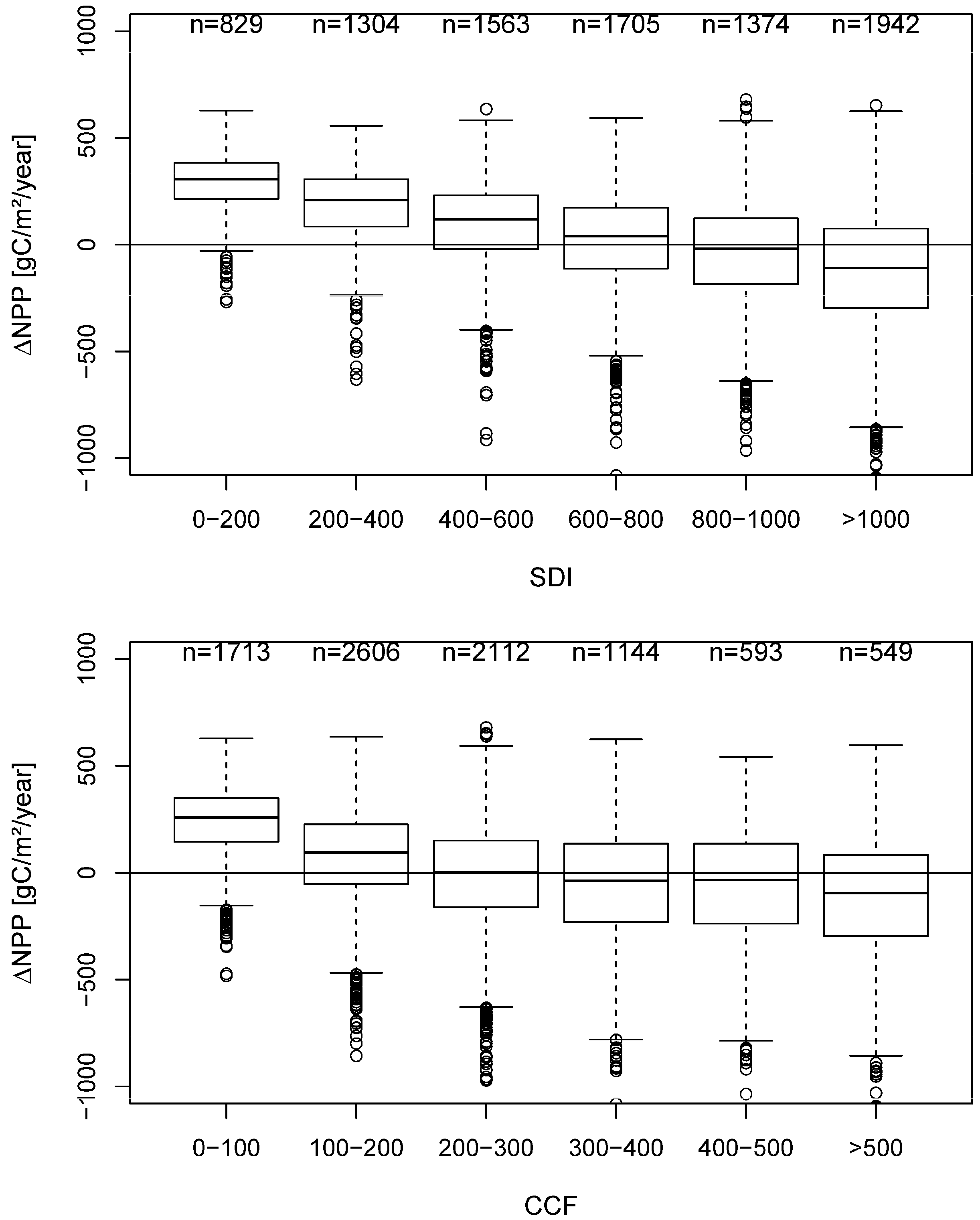
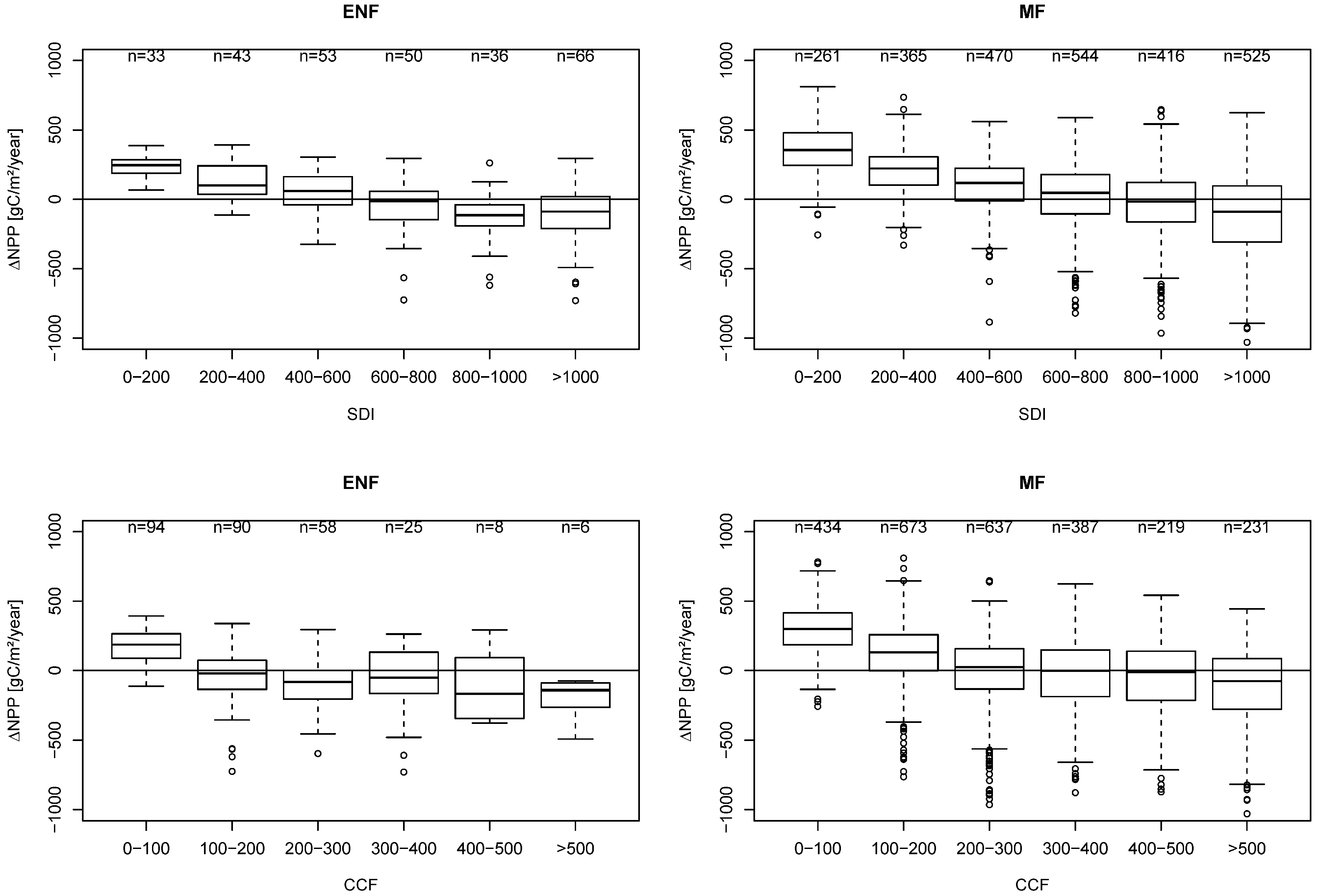
4.2. Stand Density Effects

MODIS NPP estimates vary by climate input data (ZAMG, NCEP2, GMAO) and are in general higher compared to the terrestrial NPP (NFI in Figure 2). The local daily climate data set provided by the Austrian National Weather Service (ZAMG) exhibits the lowest discrepancy versus the terrestrial NPP estimates (RMSE 276.1 gC/m2/year, difference of medians 93.5 gC/m2/year, difference of means 42.8 gC/m2/year).
Forest management reduces stand density [47,48,49,50,51,52]. Hasenauer et al. [3] suggested that stand density explains the observed discrepancies between “space-based” MODIS versus “ground-based” NPP estimates. Stand density is important considering that forest management operations change the number of trees, which directly effects the calculation of the terrestrial NPP estimates see Equations (5)–(7). In the MODIS NPP algorithm, on the other hand, forest dynamics are characterized by the two input variables FPAR and LAI, as the land cover type is kept constant. Both variables are derived from spectral properties of the vegetation, in particular the spectral signal of the red and near infrared bands [37,39]. Intensity of forest management in Austria is regulated (crown cover after thinnings of at least 60%, while clearcuts bigger than 0.5 ha need special registration and may not exceed 2 ha) [47]. Thus, it can be assumed that forest management in Austria has only a small and temporary influence on FPAR and LAI. The results of the analysis (not shown) support this as MODIS NPP show no correlation with stand density, while terrestrial NPP clearly does, which will be shown shortly.
For assessing the potential management impacts on the results we obtain for each inventory plot two stand density measures: (i) the CCF—Crown Competition Factor according to Krajicek et al. [27] Equation (11) as well as (ii) the SDI—Stand Density Index according to Reinecke [28] in Equation (14). The mean and the variations across all plots are given in Table 1.
Table 1. Summary statistics of the inventory plots for period 2007–2009 by dominant tree species. Given is mean and in brackets the data range (minimum—maximum). SDI the Stand Density Index [28], and CCF the Crown Competition Factor [27].
VariableSpruce, FirLarch, PineOther ConiferousBeechOakOther BroadleafAll
Number of plots580910011408862388648939
Age dominant trees
(a)
81
(15–175)
95
(15–175)
122
(15–175)
95
(15–175)
80
(15–165)
51
(15–175)
82
(15–175)
Elevation (m)1019
(220–2110)
914
(245–2066)
1084
(259–2212)
741
(244–1467)
377
(176–971)
544
(129–1685)
880
(129–2212)
Number of trees
(ha-1)
1029
(3–10084)
859
(4–6205)
741
(5–3544)
890
(8–9394)
692
(6–5934)
1141
(1–8917)
993
(1–10084)
Stem volume
(m³/ha)
361
(2–1672)
304
(2–1205)
268
(13–726)
329
(2–1382)
220
(8–758)
200
(2–1281)
331
(2–1672)
Basal area
(m²/ha)
36
(1–124)
33
(1–104)
35
(4–79)
33
(1–100)
25
(2–76)
25
(1–107)
34
(1–124)
SDI738
(36–2618)
665
(38–2086)
679
(48–1705)
655
(36–2066)
512
(49–1523)
553
(36–2649)
697
(36–2649)
CCF204
(7–1308)
206
(10–969)
188
(7–697)
350
(21–1622)
209
(16–625)
315
(11–1699)
229
(7–1699)
Next, we calculate the differences (∆NPP) between the “space-based” MODIS NPP (using the Austrian daily climate data ZAMG) and the “ground-based” NPP using the NFI data set. After grouping the results by CCF and SDI classes, the median and the first and third quartile of ∆NPP versus SDI and CCF class for the total data set are plotted. A direct comparison of terrestrial inventory plots with a MODIS pixel requires the assumption that a plot is actually representative for an area, which is discussed and questioned by previous research [48,49]. However, it allows us to track the effect of stand variables, which would be otherwise impossible.
A distinct stand density related trend is visible with an overestimation of the terrestrial NPP by MODIS NPP at low stand density and an underestimation at high stand density, which is consistent whether using SDI or CCF (Figure 3).
The MODIS NPP algorithm uses information on the land cover or vegetation type provided by the classification system of the University of Maryland (MODIS Collection 5 global land cover) [8,40]. In total, there are 14 land cover classes, of which five deal with forests and characterize the biophysical properties expressed by the parameters of the Biome Property Look-Up-Tables (BPLUT) [7,8]. These land cover types represent different tree species groups [40] and, due to different coefficients in the BPLUT, affect the MODIS NPP results [8]. Thus, next we are interested if the observed stand density related trends (Figure 3) may differ to MODIS land cover types.
Austria consists of a fragmented landscape, varying forest ownership and distinct historical management impacts. Consequently, many of our 3 × 3 km areas (nine pixels) include several forest land cover classes. To avoid any impact of this “mixture effect” we select only plots which feature nine pixels with only one MODIS land cover type. The land cover types “deciduous needleleaf forest” and “evergreen broadleaf forest” are excluded as there are very few pixel patches that have this land cover type exclusively (one for deciduous needleleaf forest, two for evergreen broadleaf forest).
Figure 3. Difference between MODIS NPP and NFI NPP (MODIS minus NFI) grouped by stand density measures: SDI (top); CCF (bottom). Properties of illustration analogous to Figure 2.
Remotesensing 07 03878 g003
The results for the “deciduous broadleaf forest” (not shown) are similar. To summarize, the results using plots with only one biome type exhibit the same trend when using all data (Figure 3): overestimation of terrestrial NPP by MODIS NPP at low stand density and underestimation at high stand density, which is consistent for both stand density measures (Figure 4).
Figure 4. Difference between MODIS NPP and NFI NPP (MODIS minus NFI) grouped by MODIS land cover types (ENF = evergreen needleleaf forest, MF = mixed forest) and stand density measures: SDI (top); CCF (bottom). Properties of illustration analogous to Figure 2.
Remotesensing 07 03878 g004

4.3. Addressing Stand Density Effects

The results in Figure 3 and Figure 4 show a clear stand density related trend. We apply a logarithmic trend curve to correct for stand density effects similar to Hasenauer et al. [3]:
Δ N P P = a + b × ln ( S D I ) ± ε
Δ N P P = a + b × ln ( C C F ) ± ε
a and b are the corresponding coefficient estimates and ɛ the remaining error and all other variables as previously defined. We apply Equations (15) and (16) to all data and again separately for the three MODIS forest land cover types relevant for Austrian forests (“evergreen needleleaf forest”, “mixed forest” and “deciduous broadleaf forest”. Note that the stand density measures SDI and CCF are calculated based on the stand situation at the end of the growth period. Plotting the results of the fitted trend curves show that all exhibit the same pattern whether they are grouped according to SDI or CCF (left images in Figure 5). The regression results are given in Table 2.
Figure 5. Scatterplots of NPP difference (∆NPP) and stand density dependent trend curves using SDI (top left) and CCF (bottom left), the trend curves are calculated for MODIS forest land cover types separately (ENF = evergreen needleleaf forest, DBF = deciduous broadleaf forest, MF = mixed forest) and for all land cover types together (all). The images on the right side (Corr. ∆NPP) show the NPP difference after correcting for stand density given by the trend lines using all plots (all).
Remotesensing 07 03878 g005
Table 2. Coefficients and statistics of trend curves displayed in Figure 5 a,b coefficients for Equations (15) and (16), SE standard error of coefficients, r2 coefficient of determination, n degrees of freedom.
Depending Variable aSE abSE bn
SDIENF908.383.0−143.013.10.30277
DBF1265.8194.7−192.231.60.3471
MF1203.338.1−181.36.00.262516
all1181.019.4−178.73.00.288716
CCFENF694.860.0−141.312.20.33277
DBF951.3145.1−159.526.50.3471
MF841.930.1−148.830.10.212516
all812.415.1−147.62.90.228716
A variance analysis reveal no significant differences in the parameter estimates a and b given in Table 2 between the major forest biome types represented by the MODIS land cover types. This suggests that for Austrian forests no biome type specific parameters are needed (Figure 5).
We remove the stand density bias from MODIS NPP using Equation (15), where a equals 1181.0 and b −178.7, and Equation (16), where a equals 812.4 and b −147.6 (Table 2). The detrended MODIS NPP features a mean of 515.5 gC/m2/year, standard deviation 181.7 gC/m2/year and compared to terrestrial NPP a RMSE of 227.8 gC/m2/year. After removing the stand density related trend, the difference between the two NPP assessment methods do not exhibit a bias as shown in the right-hand images in Figure 5 (SDI r2 ≤ 0.01, CCF r2 ≤ 0.01) than when using the original MODIS NPP results on the left side of Figure 5.

4.4. Consistency of the NPP Estimates across Scales

From the distinct stand density related trend in Figure 4 and Figure 5, we learn that stand density needs to be taken into consideration to provide consistent and comparable results across scales. To ensure that our findings are also consistent across the heterogeneity of the forests across Austria, we test our data for potential variations according to key forest site and stand parameters: (i) ecoregion; (ii) dominant tree species; (iii) mean stand age and (iv) elevation of a given forest inventory plot.
Austria has very distinct biogeographic growth conditions due to the east-west alignment of the Alps. According to Kilian et al. [31], these differences lead to nine typical ecoregions (see Figure 1), which are characterized by similar environmental, macro-climatic and geological conditions leading to differences in the potential vegetation.
Ecoregions strongly affect the species distribution. Thus, we next group our data by dominant tree species according to the main relative proportion of the basal area at a given inventory plot (see data section). Norway Spruce and Silver Fir, as more shade-tolerant species, are combined in one group (PA + AA). The light demanding tree species Scots Pine and European Larch form the group (PS + LD) and the group “other C” combines all other coniferous trees. The broadleaf species groups are the Common Beech (FS), the Oak (QS) and other B, which summarizes all other broadleaf species. The left images in Figure 6 show the difference between MODIS and terrestrial NPP estimates grouped by ecoregion. The differences are in general positive, both for ecoregions and tree species, before correcting for stand density. The right images show that correcting for stand density reduces this (Figure 6).
Austrian forests grow across a large gradient in elevation, which affects species and growing conditions. Again, we also group all our data by the following elevation classes: (i) <500 m; (ii) 500–1000 m; (iii) 1000–1500 m; (iv) 1500–2000 m and (v) >2000 m in elevation. The same procedure is applied for the mean stand age at a given inventory plot to assess if any age related influences of our findings exist. The six age classes across all data are: (i) <30 years; (ii) 30–60; (iii) 60–90; (iv) 90–120; (v) 120–150; and (vi) >150 years. The same pattern as in the previous Figure 6 is apparent in Figure 7 as well.
Figure 6. Difference between MODIS NPP and NFI NPP (MODIS minus NFI) grouped by ecoregions (top) and dominant tree species (bottom). Left original MODIS NPP (∆NPP) is used, right the detrended MODIS NPP (Corr. ∆NPP) is used. Properties of illustration analogous to Figure 2.
Remotesensing 07 03878 g006
Figure 7. Difference between MODIS NPP and NFI NPP (MODIS minus NFI) grouped by elevation (top) and mean stand age (bottom). Left original MODIS NPP (∆NPP) is used, right the detrended MODIS NPP (Corr. ∆NPP) is used. Properties of illustration analogous to Figure 2.
Remotesensing 07 03878 g007

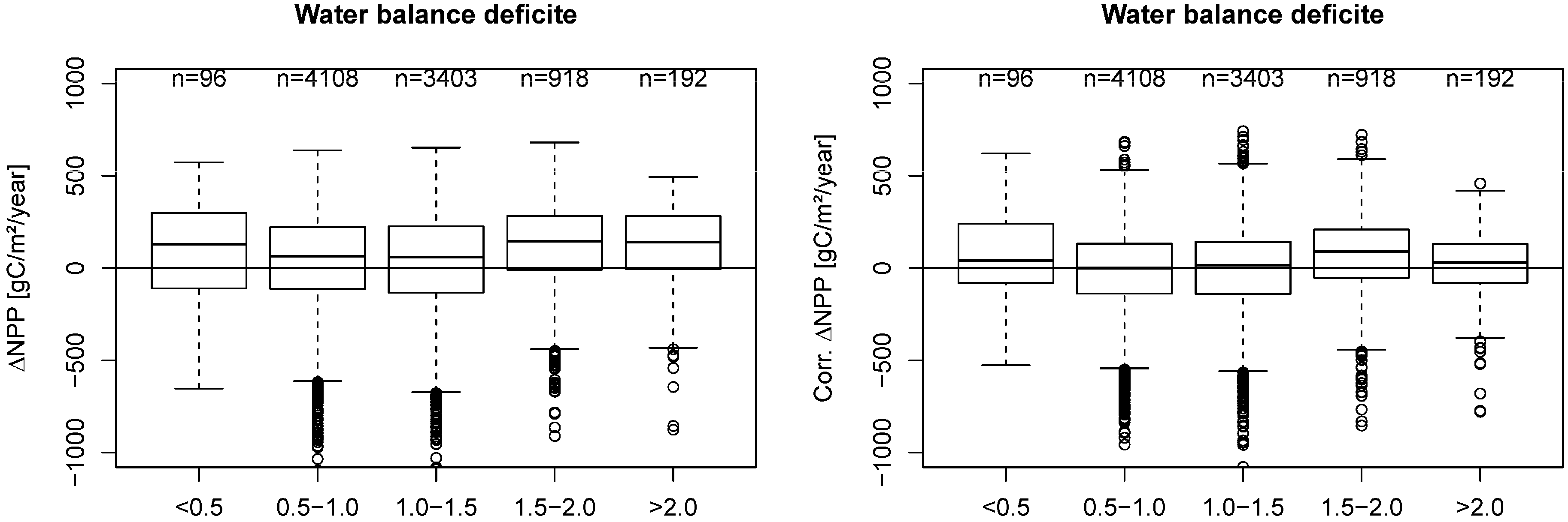
4.5. Effect of Water Availability

Water availability is an important driver of tree productivity. Within the MODIS NPP calculations [50], this is an integral part because daily climate data are required for predicting both GPP and NPP. In a previous study by Pan et al. [2], similar discrepancies in comparing the “space-based” MODIS NPP with “ground-based” terrestrial NPP were reported. Pan et al. [2] concluded that water availability may be a limiting factor and proposed an “available soil water index” for improving and/or “correcting” MODIS NPP computations compared to terrestrial data. To test this hypothesis and analyze the effect of the water availability on our data, a water balance deficit index is calculated for each inventory plot as an estimate for water limitation according to the following procedure:
W B D = E T 0 / P
E T 0 = p × ( 0.46 × T + 8 ) × 365
WBD is the water balance deficit index which is the ratio of ET0 potential evapotranspiration and P precipitation with ET0 [mm] of the period 2000–2010 estimated with the method of Blaney-Criddle [51] and P the mean annual precipitation 2000–2010 [mm]. p is a function of latitude (p = 0.2729 for a latitude of 47.5° N) and T the mean annual temperature between 2000 and 2010 [°C]. Values of WBD less than 1 indicate a lack in available water, while values higher 1 exhibit water availability greater than evapotranspiration. All data are grouped into five WBD-classes: (i) <0.5; (ii) 0.5–1.0; (iii) 1.0–1.5; (iv) 1.5 – 2.0 and (v) <2.0.
Figure 8 shows a consisted overestimation of terrestrial NPP by MODIS NPP throughout the different WBD-classes when using the original MODIS NPP. The right image in Figure 8 shows that addressing stand density effects reduces this overestimation substantially.
Figure 8. Difference between MODIS NPP and NFI NPP (MODIS minus NFI) grouped by Water balance deficit. Left original MODIS NPP (∆NPP) is used, right the detrended MODIS NPP (Corr. ∆NPP) is used. Properties of illustration analogous to Figure 2.
Remotesensing 07 03878 g008

5. Discussion

Obtaining daily local climate data (Austrian National Weather Centre ZAMG) for running the MOD17 algorithm reflects the heterogenity of the Austrian landscape more realistically and thus improves the resulting predictions [15]. The ZAMG data set uses more than 200 daily weather stations across Austria while the NCEP2 (NCEP_DOE_II) [42] and GMAO (NASA Global Modeling and Assimilation Offices) [41] include less than 40 stations. In addition, the spatial resolution of the ZAMG data set is at 0.0083 × 0.0083° (approx. 1 × 1 km). This resolution is more detailed than the two global climate data sets GMAO (0.5 × 0.67°), and NCEP2 (1.875 × 1.875°). This is an additional explanation for the higher accuracy in the local data set. Since the NPP is strongly driven by daily climate data [44] the variation of the resulting predictions using the Austrian local climate data set (ZAMG) is higher but better reflects the existing growing conditions (Figure 2).
The NPP estimates derived from 8939 plots of the National Austrian Forest Inventory (NFI) exhibit an Austrian average of 486.3 gC/m2/year (standard deviation 244.3 gC/m2/year). Applying the MODIS NPP algorithm using the local Austrian climate data (ZAMG) result in an average of 579.8 gC/m2/year (standard deviation 113.4 gC/m2/year). This is a difference between the means of 93.5 gC/m2/year.
Such differences may have several reasons. For instance, the BPLUTs might not be appropriate for European forest conditions. The difference could also be explained by inconsistency in the definition of NPP (inventory data represent trees with dbh > 5 cm, MODIS LAI all vegetation on a 1 × 1 km pixel). Other issues could be missing fineroot turnover rates in terrestrial NPP calculations, missing carbon increment of trees that died between the inventory measurements or differences in the spatial resolution of the two products. The terrestrial NPP estimates, SDI and CCF, are calculated based on the stem numbers in Equations (5)–(7). Thus, any variation in SDI or CCF directly reflects differences in the coverage of the forest area with trees. In our study of Austrian forests, we assume that the detected differences in MODIS versus terrestrial NPP (see Figure 3 and Figure 4) estimates are mainly caused by forest management. However, other events also result in changes to stand density (e.g., wind, drought stress, etc.). The observed trend by SDI [26] and CCF [27] (Figure 3 and Figure 4) and the fact that no other analyzed variable (Figure 6, Figure 7 and Figure 8) can explain the detected apparent deviations of the two NPP estimates supports the hypothesis of Hasenauer et al. [3]. Our results thus coincide with Hasenauer et al. [3], that MODIS NPP estimates provide the productivity of fully stocked forests, which are represented only by forest areas without recent changes in stand density.
Forest management, such as thinning operations, instantly reduces volume increment per unit area but concentrates the remaining volume increment to fewer trees [52]. Stand density therefore strongly affects tree diameter development. Terrestrial NPP estimates based on diameter or height data are directly affected by any changes in stand density, while the NPP estimates provided by the MODIS NPP algorithm are not. As long as interventions do not strongly reduce the spectral signal of red and near infrared—the two bands used to derive the MODIS inputs FPAR and LAI—forest management is not well detected by satellite-driven NPP estimates (see Figure 3).
The stand density pattern is also consistent when plotting only the results for each of the major vegetation or biome types represented by the MODIS land cover types (Figure 4). In this study, regression analysis and exponential trend curves are used to quantify the stand density related trend similar to Hasenauer et al. [3]. The resulting regression curves fitted using SDI and CCF in Equations (15) and (16) exhibit a consistent trend, no matter whether fitted by biome type or for all available plots. No clustering effect by biome type is evident, suggesting that one density-driven correction function adjusts for the bias in the NPP predictions across scales (Table 2, Figure 5).
Both competition measures (SDI and CCF) show a very similar behavior (see Figure 3, Figure 4 and Figure 5). However, for this dataset, SDI gives a slightly higher coefficient of determination (Table 2) and seems to better address the recorded competition that exists within Austrian National Forest inventory plots. As shown in Figure 6 and Figure 7, ignoring stand density effects will cause overestimation by MODIS NPP estimates by ecoregions and dominant tree species (see Figure 6), elevation and mean stand age (see Figure 7). Applying the correction function leads to a substantial improvement in the consistency of the different NPP results, and consistent and unbiased results across multiple scales can be expected.
The fact that terrestrial NPP overestimates MODIS NPP at high stand densities (SDI > 1000 or CCF > 500) can be explained with the variable “plot size” of the inventory plots according to the breast height diameter of the trees on a given plot [20]. Thus, the terrestrial NPP estimates based on angle count sample data may have a large random variation and this differs substantially from the terrestrial plot data for deriving NPP as outlined in Hasenauer et al. [3] who used fixed area research plots with an area of 2500 m2.
Pan et al. [2] also observed differences between MODIS and terrestrial NPP. They hypothesized that soil water constraints may be a limiting factor and proposed an “available soil water index” for adjusting MODIS NPP computations compared to terrestrial data. Our results of growth conditions in Austrian forests, however, suggest that stand density explains the observed discrepancy as the results grouped by water balance index show a systematic overestimation of terrestrial NPP by MODIS NPP (Figure 8). Correcting for stand density results in a better agreement of MODIS and terrestrial NPP across different “available soil water indices”.
One important concern of our study was if large-scale disturbances like bark beetle outbreaks or windthrow [53,54] may have had an impact on our productivity results by method. Disturbances reduce the stand density of forests in a similar manner to management. In our available data from the Austrian Forest inventory, disturbances can be detected with a recorded variable explaining the reason for sample tree death or removal [17]. There are 484 plots (5% of all plots) where, between 2007 and 2009, at least one tree with “random removal” was recorded and, thus, were affected by the disturbances between 2000 and 2002 and between 2007 and 2009. These plots have a median NPP of 464.7 gC/m2/year, which is only slightly lower than the median NPP of all 8939 plots (486.3 gC/m2/year). While disturbances might have big impacts on small scales like forest stands or single inventory plots, they only have a limited and insignificant effect as compared to the forest productivity of Austria.

6. Conclusions

The MODIS NPP model represents all forest vegetation within a 1 × 1 km resolution, assumes fully stocked forest stands and cannot effectively detect management influence in FPAR and LAI. Thus, the effect of forest management, which changes the carbon allocation patterns and, as a consequence, the tree dimensions, is not well represented by MODIS driven NPP estimates. Terrestrial NPP, on the other hand, represents only NPP of trees bigger than the diameter threshold and captures the response of trees to management and, thus, the actual carbon allocation.
Using daily local climate data with high spatial resolution improves the agreement between MODIS NPP and terrestrial NPP.
Correcting the observed stand density related bias in MODIS NPP and thus combining the “space-based” MODIS productivity estimates and “ground-based” national forest inventory data provide consistent and continuous forest productivity estimates. The corrected MODIS NPP has more agreement with forest inventory data. A better agreement of MODIS and terrestrial NPP estimates allows using MODIS for large-scale forest resource estimates in areas with forest management.
Forest productivity across large scales is of increasing interest as more demands are made on forest resources [55] as well as in the context of REDD (Reducing Emissions from Deforestation and Forest Degradation) [56]. This is of particular importance for areas where no or little terrestrial information on forest productivity is available. With this paper, we provide a conceptual outline of how realistic forest productivity estimates can be derived by combining satellite-driven NPP estimates, such as results from the MODIS NPP algorithm, with stand density estimates (using terrestrial or remote-sensing data) in order to enhance forest productivity predictions across multiple scales.

Acknowledgments

This work is part of the project “Comparing satellite versus ground driven carbon estimates for Austrian Forests” (MOTI). We are grateful for the financial support provided by the Energy Fund of the Federal State of Austria—managed by Kommunalkredit Public Consulting GmbH under contract number K10AC1K00050. MT. The NTSG work is funded by NASA Earth Observing System MODIS project (grant NNH09ZDA001N-TERRA-AQUA). We thank the editors and the anonymous reviewers for their helpful comments, which substantially improved the quality of this work. We further want to thank Adam Moreno for proof reading the manuscript.

Author Contributions

Mathias Neumann did the comparative analysis of the results, prepared images and tables and wrote the manuscript. Maosheng Zhao did the calculation of MODIS NPP using different climate data and revised the chapters on the MODIS NPP calculations. Georg Kindermann provided the tree carbon results using the Austrian forest inventory data and revised the chapters on forest inventory data and carbon estimation method. Hubert Hasenauer provided the climate data for Austria and revised the whole manuscript.

Conflicts of Interest

The authors declare no conflict of interest.

Appendix

Carbon estimation and calculation of crown width using NFI data

The carbon increment calculation require carbon estimates for each tree on a given inventory plot. For our study, we use the same method as applied by the Institute of Forest Inventory, Federal Research Centre for Forest, the agency responsible for the National Forest Inventory in Austria. The total dry carbon tree estimate of a single tree, Ci, is calculated as follows:
C i = C C × ( d s m + d b m + d f m + d r m )
where CC is the carbon content and considered to be 0.5 for all species [26], dsm is the dry stem mass, dbm the dry branch mass, dfm the dry foliage mass and drm the dry root mass.
Dry stem biomass (dsm) is calculated using stem volume and species-specific conversion factors. Stem volume (Vtree) is derived from the tree measurements diameter at breast height (dbh), total tree height (h) and the species-specific form factor (FF). The calculated volume represents the stem excluding aboveground part of the stump and the branches [17,57,58].
d s m = V t r e e × w d × 100 s f 100
V t r e e = ( d b h 200 ) 2 × π × h × F F
where Vtree is the stem volume of a single tree [m³], wd is the dry wood density [t BM/m³], sf the shrinkage factor by tree species [%], dbh the diameter at breast height (1.3 m), h the tree height, d03 the diameter at 30% of tree height and hc the crown height (height to the crown base). The form factor (FF) reduces the volume of the cylinder to the actual tree form. The Austrian Forest Inventory uses two different form factor functions: one for the trees with dbh ranging from 5–10.4 cm with the following form,
F F = c 1 + c 2 × ln 2 ( d b h ) + c 3 / h + c 4 / d b h + c 5 / d b h ² + c 6 / d b h / h + c 7 / d b h ² / h
and a second one for all trees with a dbh≥10.4 cm:
F F = c 0 + c 1 × d 03 / d b h + c 2 × ( d 03 / h ) 2 + c 3 × h / d b h + c 4 × h / d b h ² + c 5 / d b h + c 6 × h c / h
ci are species-specific parameter estimates for calculating stem volume used by the Austrian Forest Inventory given in Table A1 and Table A2 [17,57,59]. The conversion factors wd and sf according to Wagenführ and Scheiber [60] are given in Table A3. Note that for Equation (A3) dbh [cm] and h [m], while in Equations (A4,A5) the d03, dbh, hc and h [dm].
Table A1. Coefficients used in models for volume for trees with dbh 5.0–10.4 cm (Schieler [59] cited in Gabler and Schadauer [17]).
Species Namec1c2c3c4c5c6c7
Picea abies, other coniferous0.5634−0.1273−8.5502007.63310
Abies alba0.56070.1547−0.65580.0332000
Larix decidua0.48730−2.0429005.99950
Pinus sylvestris, Pinus strobus0.4359−0.01495.210900.028700
Pinus nigra0.5344−0.007600002.2414
Pinus cembra0.5257−0.03357.3894−0.1065003.3448
Fagus sylvatica, other broadleaf0.51730−13.6214009.98880
Quercus sp.0.41710.219413.32590000
Carpinus betulus0.32470.024300.23970−9.93880
Fraxinus sp., Sorbus sp., Prunus sp.0.4812−0.0149−10.831009.39360
Acer sp.0.5010−0.0352−8.071800.035200
Ulmus sp.0.4422−0.024500002.8771
Betula sp.0.4283−0.06640008.43070
Alnus sp.0.387407.17120.0441000
Populus sp.0.366401.13320.1306000
Salix sp.0.5401−0.0272−25.11450.083309.39880
Table A2. Coefficients used in models for volume for trees with dbh≥10.4 cm (Braun [57] cited in Gabler and Schadauer [17]).
Species Namec0c1c2c3c4c5c6
Picea abies, other coniferous−0.24360.827102.91E-0400.02870
Abies alba0.099100.51264.46E-0400.01600
Larix decidua−0.21980.802803.24E-0400.01840
Pinus sylvestris−0.20990.814001.96E-0400.03170
Pinus nigra, Pinus strobus−0.19290.847902.04E-0400.00690
Pinus cembra0.05010.467601.57E-0400.07610
Fagus sylvatica, other broadleaf−0.13090.6743001.67E-0400.0668
Quercus sp.0.185200.350104.77E-0400.0657
Carpinus betulus0.04210.4226004.21E-0400.0770
Fraxinus sp.−0.01980.5124004.70E-0400.0535
Acer sp.−0.02860.5655002.37E-0400.0083
Ulmus sp.−0.13900.6950003.18E-0400.0166
Betula sp.−0.07780.5682005.54E-0400.0517
Alnus sp.−0.16460.7038002.59E-0400.0589
Populus tremula−0.14560.6657004.18E-0400.0589
Populus alba−0.14380.6487005.62E-0400.0812
Populus nigra−0.08430.5928006.47E-0400.0227
Salix sp.−0.13760.6944004.59E-0400.0128
Table A3. Conversion factors for stem biomass [60].
Species Namewdsf
Picea sp.0.4111.80
Abies sp.0.4111.85
Larix sp.0.5513.20
Pinus sylvestris, other Pinus0.5111.80
Pinus nigra0.5611.80
Pinus cembra0.409.00
Pinus strobus0.379.00
Pseudotsuga menziesii0.4712.00
Taxus baccata0.648.80
Fagus sylvatica, other hardwood broadleaf0.6817.50
Carpinus betulus0.6713.60
Quercus sp.0.7518.80
Fraxinus sp.0.6713.20
Acer sp.0.5911.65
Ulmus sp.0.6412.80
Castanea sativa0.5611.45
Robinia pseudacacia0.7311.80
Prunus sp., Sorbus sp.0.5713.85
Sorbus domestica0.7117.15
Sorbus aucuparia0.6218.60
Betula sp.0.6413.95
Alnus sp.0.4913.40
Tilia sp., other softwood broadleaf0.5214.65
Populus sp.0.4511.90
Populus nigra0.4112.50
Salix sp.0.529.60
Juglans regia0.6413.70
Juglans nigra0.5612.65
Ostrya carpinifolia0.7518.80
Malus, Pyrus0.7014.40
For the remaining biomass components (dbm, dfm, drm), we use allometric biomass functions developed for Austrian forest conditions, which are also used by the Austrian National Forest Inventory.
The dry branch biomass dbm [kg] for Pinus sp. is calculated with a dbh [cm] and h [m] dependent equation [61],
d b m = 1.0366 e ( 2.8762 + 2.04516 ln ( d b h ) 0.07025 ln ( h ) )
We use equations from Ledermann and Neumann [62] for all other tree species. If height to the life crown measurements (hc) are available, models using dbh, h and hc as input variables are used according to Equation (A8). If hc is missing, models with dbh and h are used according to Equation (A7) [62]:
d b m = l 2 e b 20 + b 21 ln ( d b h ) + b 22 h d b h )
d b m = l 3 e b 30 + b 31 ln ( d b h ) + b 32 h d b h + b 33 ln ( C R )
C R = h h c h
where CR is the crown ratio and all other variables as previously defined. The species-specific parameters bi, l2 and l3 are given in Table A4.
Table A4. Coefficients used in models for biomass in branches [62].
Species Nameb20b21b22l2b30b31b32b33l3
Picea abies, other coniferous except Pinus sp.-1.16351.7459-0.94991.102-1.95762.02520.14510.91541.051
Abies alba-2.43272.0429-0.66671.105-2.96502.206600.43841.087
Fagus sylvatica, other BL-3.06882.3930-0.55481.251-3.32052.5568-0.10920.60021.212
Quercus sp.1.85540.9332-1.71501.334-1.29431.944501.21371.280
Carpinus betulus-4.41192.8913-0.43111.181-3.65982.828100.93181.130
For coniferous trees, the foliage biomass (dfm) is included in the branch biomass calculations (dbm) as outlined above. For the deciduous trees, dfm [kg] is calculated using allometric functions according to dbh. These functions are based on measurements collected by Burger [63,64] and are modified after Lexer and Hönninger [65].
d f m = a 0 × d b h a 1
The species-specific parameters ai are given in Table A5.
The root biomass (drm) in [kg] is defined as roots with a minimum diameter of 2 mm including the root stump. For Pinus sylvestris and Pinus nigra the allometric function of Offenthaler and Hochbichler [66] is used:
d r m = 0.038872 × d b h 2.066783
For all other species, the following dbh and age-dependent model is applied [67,68]:
d r m = c 0 e c 1 + c 2 ln ( d b h ) + c 3 ln 2 ( d b h ) + c 4 ln ( a g e )
dbh in [cm], age is the tree age [a], ci are species-specific parameter according to [67,68].
The species-specific parameters ci are given along with the parameters for foliage biomass in the Table A5.
Table A5. Coefficients ci used in models for biomass in roots ([67] for “Coniferous (except Pinus sp.)”, [68] for “Fagus sylvatica, other broadleaf”, [66] for “Quercus sp.” and “Carpinus betulus”) and a0 and a1 for biomass in foliage [63,64,65].
Namec0c1c2c3c4a0a1
Coniferous (except Pinus sp.)1.041−8.3504.568−0.3300.281--
Fagus sylvatica, other broadleaf1.080−4.0002.320000.0222.300
Quercus sp.1.051−3.9752.523000.1351.811
Carpinus betulus1.052−3.8482.488000.0222.300
Equation (A13) estimates maximum crown width of a tree assuming open-grown conditions for calculating CCF [27]. The species-specific parameters to calculate maximum crown width are given in Table A6.
C W i = e c 0 + c 1 ln ( d b h )
Table A6. Coefficients used for maximum crown width [29].
Namec0c1
Picea abies, other coniferous−0.32320.6441
Abies alba0.09200.5380
Larix decidua−0.33960.6823
Pinus sylvestris, other Pinus sp.−0.17970.6267
Pinus nigra−0.15700.6310
Pinus cembra−1.31540.8288
Fagus sylvatica, other broadleaf0.26620.6072
Quercus sp., Castanea sativa−0.39730.7328
Acer sp., Betula sp., Alnus sp., Populus sp., Salix sp., Ulmus sp.0.41800.5285
Fraxinus sp., Robinia, sp. Prunus sp. Sorbus sp.0.13660.6183
Tilia sp.0.17830.5665

References

  1. Shvidenko, A.; Schepaschenko, D.; McCallum, I.; Santoro, M.; Schmullius, C. Use of remote sensing products in a terrestrial ecosystems verified full carbon account: Experiences from Russia. In Proceedings of the International Institute for Applied Systems Analysis: Earth Observation for Land-Atmosphere Interaction Science, Frascati, Italy, 3–5 November 2010.
  2. Pan, Y.; Birdsey, R.; Hom, J.; McCullough, K.; Clark, K. Improved estimates of net primary productivity from MODIS satellite data at regional and local scales. Ecol. Appl. 2006, 16, 125–132. [Google Scholar] [CrossRef] [PubMed]
  3. Hasenauer, H.; Petritsch, R.; Zhao, M.; Boisvenus, C.; Running, S.W. Reconciling satellite with ground data to estimate forest productivity at national scales. For. Ecol. Manag. 2012, 276, 196–208. [Google Scholar] [CrossRef]
  4. Tomppo, E.; Gschwantner, T.; Lawrence, M.; McRoberts, R.E. National Forest Inventories: Pathways for Common Reporting; Springer: Berlin, Germany, 2010; p. 610. [Google Scholar]
  5. Schadauer, K.; Gschwantner, T.; Gabler, K. Austrian National Forest Inventory: Caught in the Past and Heading toward the Future. In Proceedings of the Seventh Annual Forest Inventory and Analysis Symposium, Washington, DC, USA, 3–6 October 2005; pp. 47–53.
  6. Hasenauer, H.; Eastaugh, C.S. Assessing forest production using terrestrial monitoring data. Int. J. For. Res. 2012. [Google Scholar] [CrossRef]
  7. Running, S.; Nemani, R.; Heinsch, F.; Zhao, M.; Reeves, M.; Hashimoto, H. A continuous satellite-derived measure of global terrestrial primary production. BioScience 2004, 54, 547–560. [Google Scholar] [CrossRef]
  8. Zhao, M.; Running, S.W. Drought-induced reduction in global terrestrial net primary production from 2000 through 2009. Science 2010, 329, 940–943. [Google Scholar]
  9. Monteith, J. Solar radiation and productivity in tropical ecosystems. J. Appl. Ecol. 1972, 9, 747–766. [Google Scholar] [CrossRef]
  10. Thornton, P.E.; Running, S.; White, M. Generating surfaces of daily meteorological variables over large regions of complex terrain. J. Hydrol. 1997, 190, 214–251. [Google Scholar] [CrossRef]
  11. Van Tuyl, S.; Law, B.E.; Turner, D.P.; Gitelman, A.I. Variability in net primary production and carbon storage in biomass across Oregon forests—An assessment integrating data from forest inventories, intensive sites, and remote sensing. For. Ecol. Manag. 2005, 209, 273–291. [Google Scholar] [CrossRef]
  12. Waring, R.H.; Milner, K.S.; Jolly, W.M.; Phillips, L.; McWethy, D. Assessment of site index and forest growth capacity across the Pacific and Inland Northwest USA with MODIS satellite-derived vegetation index. For. Ecol. Manag. 2006, 228, 285–291. [Google Scholar] [CrossRef]
  13. Muukkonen, P.; Heiskanen, J. Biomass estimation over a large area based on standwise forest inventory data and ASTER and MODIS satellite data: A possibility to verify carbon inventories. Remote Sens. Environ. 2007, 107, 617–624. [Google Scholar] [CrossRef]
  14. Härkönen, S.; Lehtonen, A.; Eerikäinen, K.; Mäkelä, A. Estimating forest carbon fluxes for large regions based on process-based modelling, NFI data and Landsat satellite images. For. Ecol. Manag. 2011, 262, 2364–2377. [Google Scholar] [CrossRef]
  15. Eenmäe, A.; Nilson, T.; Lang, M. A note on meteorological variables related trends in the MODIS NPP product for Estonia. For. Stud./Metsanduslikud. Uurim. 2011, 55, 60–63. [Google Scholar]
  16. Fang, H.; Wei, S.; Liang, S. Validation of MODIS and CYCLOPES LAI products using global field measurement data. Remote Sens. Environ. 2012, 119, 43–54. [Google Scholar] [CrossRef]
  17. Gabler, K.; Schadauer, K. Methods of the Austrian forest inventory 2000/02 origins, approaches, design, sampling, data models, evaluation and calculation of standard error. Available online: http://bfw.ac.at/rz/bfwcms.web?dok=7518 (accessed on 30 March 2015).
  18. He, L.; Chen, J.M.; Pan, Y.; Birdsey, R.; Kattge, J. Relationships between net primary productivity and forest stand age in U.S. forests. Glob. Biogeochem. Cycles 2012, 26, 1–19. [Google Scholar] [CrossRef]
  19. Liu, C.; Westman, C.; Berg, B.; Kutsch, W.; Wang, G.Z.; Man, R.; Ilvesniemi, H. Variation in litterfall-climate relationships between coniferous and broadleaf forests in Eurasia. Glob. Ecol. Biogeogr. 2004, 13, 105–115. [Google Scholar] [CrossRef]
  20. Bitterlich, W. Die Winkelzaehlprobe. Allg. For. Holzwirtsch. Ztg. 1948, 59, 4–5. [Google Scholar]
  21. Englisch, M.; Karrer, G.; Mutsch, F. Österreichische Waldboden-Zustandsinventur. Teil 1: Methodische Grundlagen. Mitt. Forstichen Bundesver. Wien. 1992, 168, 5–22. [Google Scholar]
  22. Schieler, K. Methode der Zuwachsberechnung der Oesterreichischen Waldinventur. Ph.D. Thesis, University of Natural Resources and Applied Life Sciences, Institute of Forest Growth, Vienna, Austria, 1997; p. 92. [Google Scholar]
  23. Van Deusen, P.C.; Dell, T.R.; Thomas, C.E. Volume Growth Estimation from Permanent Horizontal Points. For. Sci. 1986, 32, 415–422. [Google Scholar]
  24. Eastaugh, C.S.; Hasenauer, H. Biases in Volume Increment Estimates Derived from Successive Angle Count Sampling. For. Sci. 2013, 59, 1–14. [Google Scholar]
  25. Martin, G.L. A method for estimating ingrowth on permanent horizontal sample points. For. Sci. 1982, 28, 110–114. [Google Scholar]
  26. Intergovernmental Panel on Climate Change, Good Practice Guidance for Land Use, Land-Use Change and Forestry; Institute for Global Environmental Strategies (IGES): Hayama, Japan, 2003; p. 590.
  27. Krajicek, J.E.; Brinkman, K.A.; Gingrich, S.F. Crown competition—A measure of density. For. Sci. 1961, 1, 35–42. [Google Scholar]
  28. Reinecke, L.H. Prefecting a stand density index for even-aged forest. J. Agric. Res. 1933, 46, 627–638. [Google Scholar]
  29. Hasenauer, H. Dimensional relationships of open-grown trees in Austria. For. Ecol. Manag. 1997, 96, 197–206. [Google Scholar] [CrossRef]
  30. Hasenauer, H.; Burkhart, H.; Sterba, H. Variation in potential volume yield of loblolly pine plantations. For. Sci. 1994, 40, 162–176. [Google Scholar]
  31. Kilian, W.; Müller, F.; Starlinger, F. Die forstlichen Wuchsgebiete Österreichs—Eine Naturraumgliederung nach waldökologischen Gesichtspunkten. Available online: http://bfw.ac.at/030/2377.html (accessed on 27 March 2015).
  32. Hasenauer, H.; Merganičová, K.; Petritsch, R.; Pietsch, S.A.; Thornton, P.E. Validating daily climate interpolations over complex terrain in Austria. Agric. For. Meteorol. 2003, 119, 87–107. [Google Scholar] [CrossRef]
  33. Eastaugh, C.S.; Petritsch, R.; Hasenauer, H. Climate characteristics across the Austrian forest estate from 1960 to 2008. Aust. J. For. Sci. 2010, 127, 133–146. [Google Scholar]
  34. Thornton, P.E.; Hasenauer, H.; White, M.A. Simultaneous estimation of daily solar radiation and humidity from observed temperature and precipitation: An application over complex terrain in Austria. Agric. For. Meteorol. 2000, 104, 255–271. [Google Scholar] [CrossRef]
  35. Petritsch, R.; Hasenauer, H. Climate input parameters for real-time online risk assessment. Nat. Hazards 2011, 59, 1–14. [Google Scholar] [CrossRef]
  36. Zhao, M.; Heinsch, F.A.; Nemani, R.R.; Running, S.W. Improvements of the MODIS terrestrial gross and net primary production global data set. Remote Sens. Environ. 2005, 95, 164–175. [Google Scholar] [CrossRef]
  37. Wang, Y.; Woodcock, C.E.; Buermann, W.; Stenberg, P.; Voipio, P.; Smolander, H.; Hame, T.; Tian, Y.; Hu, J.; Knyazikhin, Y.; Myneni, R.B. Evaluation of the MODIS LAI algorithm at a coniferous forest site in Finland. Remote Sens. Environ. 2004, 91, 114–127. [Google Scholar] [CrossRef]
  38. Tan, B.; Woodcock, C.; Hu, J.; Zhang, P.; Ozdogan, M.; Huang, D.; Yang, W.; Knyazikhin, Y.; Myneni, R. The impact of gridding artifacts on the local spatial properties of MODIS data: Implications for validation, compositing, and band–to–band registration across resolutions. Remote Sens. Environ. 2006, 105, 98–114. [Google Scholar] [CrossRef]
  39. Yang, W.; Tan, B.; Huang, D.; Rautiainen, M.; Shabanov, N.V.; Wang, Y.; Privette, J.L.; Hummerich, K.F.; Fensholt, R.; Sandolt, I.; et al. MODIS leaf area index products: From validation to algorithm improvement. IEEE Trans. Geosci. Remote Sens. 2006, 44, 1885–1898. [Google Scholar] [CrossRef]
  40. Friedl, M.; Sulla-Menashe, D.; Tan, B.; Schneider, A.; Ramankutty, N.; Sibley, A.; Huang, X. MODIS Collection 5 global land cover: Algorithm refinements and characterization of new datasets. Remote Sens. Environ. 2010, 114, 168–182. [Google Scholar] [CrossRef]
  41. Ma, L.; Zhang, T.; Li, Q.; Frauenfeld, O.W.; Qin, D. Evaluation of ERA-40, NCEP-1, and NCEP-2 reanalysis air temperatures with ground-based measurements in China. J. Geophys. Res. 2008, 113, 1–15. [Google Scholar]
  42. Kanamitsu, M.; Ebisuzaki, W.; Woollen, J.; Yang, S.K.; Hnilo, J.J.; Fiorino, M.; Potter, G.L. NCEP-DOE AMIP-II reanalysis (R-2). Bull. Am. Meteorol. Soc. 2002, 83, 1631–1643. [Google Scholar] [CrossRef]
  43. Weng, Q. Global Urban Monitoring and Assessment through Earth Observation; CRC Press: Boca Raton, FL, USA, 2014; p. 440. [Google Scholar]
  44. Zhao, M.; Running, S.W.; Nemani, R.R. Sensitivity of moderate resolution imaging spectroradiometer (MODIS) terrestrial primary production to the accuracy of meteorological reanalyses. J. Geophys. Res. 2006, 111, 1–13. [Google Scholar] [PubMed]
  45. Bruce, D. Yield Differences between Research Plots and Managed Forests. J. For. 1977, 75, 14–17. [Google Scholar]
  46. Hradetzky, J. Concerning the precision of growth estimation using permanent horizontal point samples. For. Ecol. Manag. 1995, 71, 203–210. [Google Scholar] [CrossRef]
  47. Austrian Forest Act (Österreichisches Forstgesetz). Available online: https://www.ris.bka.gv.at/ (accessed on 4 February 2015).
  48. Eastaugh, C.; Hasenauer, H. Improved estimates of per-plot basal area from angle count inventories. Forests 2014, 7, 178–185. [Google Scholar]
  49. Seidl, R.; Eastaugh, C.S.; Kramer, K.; Maroschek, M.; Reyer, C.; Socha, J.; Vacchiano, G.; Zlatanov, T.; Hasenauer, H. Scaling issues in forest ecosystem management and how to address them with models. Eur. J. For. Res. 2013, 132, 653–666. [Google Scholar] [CrossRef]
  50. Zhang, K.; Kimball, J.S.; Mu, Q.; Jones, L.A.; Goetz, S.J.; Running, S.W. Satellite based analysis of northern ET trends and associated changes in the regional water balance from 1983 to 2005. J. Hydrol. 2009, 379, 92–110. [Google Scholar] [CrossRef]
  51. Blaney, H.F.; Criddle, W.D. Determining Water Requirements in Irrigated Areas from Climatological and Irrigation Data; Technical Paper; United States Department of Agriculture: Washington, WA, USA, 1950; Volume 96, p. 44.
  52. Assmann, E. The Principles of Forest Yield Study; Pergamon Press: New York, NY, USA, 1970; p. 506. [Google Scholar]
  53. Seidl, R.; Rammer, R.; Jäger, D.; Lexer, M.J. Impact of bark beetle (Ips. typographus L.) disturbance on timber production and carbon sequestration in different management strategies under climate change. For. Ecol. Manag. 2008, 256, 209–220. [Google Scholar] [CrossRef]
  54. Seidl, R.; Fernandes, P.M.; Fonseca, T.F.; Gillet, F.; Jönsson, A.M.; Merganicova, K.; Netherer, S.; Arpaci, A.; Bontemps, J.D.; Bugmann, H.; et al. Modelling natural disturbances in forest ecosystems: A review. Ecol. Model. 2010, 222, 903–924. [Google Scholar] [CrossRef]
  55. Pan, Y.; Birdsey, R.A.; Fang, J.; Houghton, R.; Kauppi, P.E.; Kurz, W.A.; Phillips, O.L.; Lewis, S.L.; Canadell, J.G.; Ciais, P.; et al. A large and persistent carbon sink in the world’s forests. Science 2011, 333, 988–992. [Google Scholar] [CrossRef] [PubMed]
  56. Angelsen, A. Realising REDD+ National Strategy and Policy Options; CIFOR: Bogor, Indonesia, 2009; p. 390. [Google Scholar]
  57. Braun, R. Österreichische Forstinventur. Methodik der Auswertung und Standardfehler-Berechnung. Mitt. Forstl. Bundesver. Wien. 1969, 84, 1–60. [Google Scholar]
  58. Pollanschütz, J. Formzahlfunktionen der Hauptbaumarten Österreichs. Inf. Forstl. Bundesver. Wien. 1974, 153, 341–343. [Google Scholar]
  59. Schieler, K. Methodische Fragen in Zusammenhang mit der österreichischen Forstinventur. Master Thesis, University of Natural Resources and Applied Life Sciences, Institute of Forest Growth, Vienna, Austria, 1988; p. 99. [Google Scholar]
  60. Wagenführ, R.; Scheiber, C. Holzatlas, 2nd Ed. ed; VEB Fachbuchverlag: Leibzig, Germany, 1985; p. 690. [Google Scholar]
  61. Hochbichler, E.; Bellos, P.; Lick, E. Biomass functions for estimating needle and branch biomass of spruce (Picea abies) and Scots pine (Pinus sylvestris) and branch biomass of beech (Fagus sylvatica) and oak (Quercus robur and petrea). Aust. J. For. Sci. 2006, 123, 35–46. [Google Scholar]
  62. Ledermann, T.; Neumann, M. Biomass equations from data of old long-term experimental plots. Aust. J. For. Sci. 2006, 123, 47–64. [Google Scholar]
  63. Burger, H. Holz, Blattmenge und Zuwachs. VIII. Mitteilung. Die Eiche. Mitt. Schweiz. Anst. Forstl. Vers. 1947, 25, 211–279. [Google Scholar]
  64. Burger, H. Holz, Blattmenge und Zuwachs. X. Mitteilung. Die Buche. Mitt. Schweiz. Anst. Forstl. Vers. 1949, 26, 419–468. [Google Scholar]
  65. Lexer, M.J.; Hoenninger, K. A modified 3D-patch model for spatially explicit simulation of vegetation composition in heterogeneous landscapes. For. Ecol. Manag. 2001, 144, 43–65. [Google Scholar] [CrossRef]
  66. Offenthaler, I.; Hochbichler, E. Estimation of root biomass of Austrian forest tree species. Aust. J. For. Sci. 2006, 123, 65–86. [Google Scholar]
  67. Wirth, C.; Schumacher, J.; Schulze, E.D. Generic biomass functions for Norway spruce in Central Europe—A meta-analysis approach toward prediction and uncertainty estimation. Tree Physiol. 2004, 24, 121–139. [Google Scholar] [CrossRef] [PubMed]
  68. Bolte, A.; Rahmann, T.; Kuhr, M.; Pogoda, P.; Murach, D.; von Gadow, K. Relationships between tree dimension and coarse root biomass in mixed stands of European beech (Fagus sylvatica L.) and Norway spruce (Picea abies[L.] Karst.). Plant Soil 2004, 264, 1–11. [Google Scholar] [CrossRef]

