Article

Geometric Quality Analysis of AVHRR Orthoimages

by
Sultan Kocaman Aksakal
1,*,†,
Christoph Neuhaus
2,
Emmanuel Baltsavias
3 and
Konrad Schindler
3
1
Department of Geomatics Engineering, Hacettepe University, Ankara 06800, Turkey
2
Department of Geography, University of Bern, CH-3012 Bern, Switzerland
3
ETH Zurich, Institute of Geodesy and Photogrammetry, CH-8093 Zurich, Switzerland
*
Author to whom correspondence should be addressed.
The work has been done while she was at ETH Zurich.
Remote Sens. 2015, 7(3), 3293-3319; https://doi.org/10.3390/rs70303293
Submission received: 15 September 2014 / Revised: 6 March 2015 / Accepted: 9 March 2015 / Published: 23 March 2015

Abstract

:
The geometric accuracy of 2008 AVHRR orthoimages from Metop-A, NOAA-17 and NOAA-18 satellites over Switzerland have been investigated here. The methods employed in the study are fully automated, with an accuracy of 0.1–0.2 pixels, however, blunders do occur and this requests a careful blunder detection approach. The investigations include analysis of relative, absolute and band-to-band registration (BBR) accuracy. Regarding relative accuracy, thousands of points are matched between Metop-A, NOAA-17 and NOAA-18 images of the same day. The accuracy is quite high with mean shifts between 0.2 and 0.4 pixels. Systematic stripes have been observed when NOAA-18 images are involved in matching. In spite of many efforts to find the source of this error, no explanation could be found. In addition, large shifts up to 2.9 pixels on some days between September and December 2008 were observed. Regarding absolute accuracy, digitized lakes as reference polygons have been used and a subpixel lake matching method has been applied. The mean shifts generally fulfilled EUMETSAT and GCOS specifications, although some partial results exceed them, especially for Metop-A. Regarding BBR accuracy, six multispectral bands have been compared, also with point matching. The EUMETSAT specification is 0.1 km, however, this specification refers to original images, not orthoimages. Taking also into account the matching errors of 0.1 km, the EUMETSAT specifications are in principle fulfilled in all cases except matching of Metop-A and NOAA-17 Band-2 images with Bands 4 and 5. The overall work showed that although, in general, accuracies are high and fulfill specifications, errors exceeding the specifications can occur and vary depending on the satellite used, time and location. Such errors influence subsequent geometric or thematic processing; thus, an automated and permanent quality control of such images should be executed.

Graphical Abstract

1. Introduction

1.1. Motivation and Background

A research project has been carried out at ETH Zurich in cooperation with the Swiss GCOS (Global Climate Observing System) office at MeteoSwiss, which coordinates the GCOS activities in Switzerland [1,2]. The GCOS is a long-term program aiming at providing systematic observations required for monitoring and improving the understanding of the climate system, detecting climate changes, and assessing their impacts and sponsored by WMO (World Meteorological Organization), the Intergovernmental Oceanographic Commission (IOC) of the UNESCO, the UNEP (UN Environmental Programme), and the ICSU (International Council of Science) [3]. GCOS has defined the Essential Climate Variables (ECVs) and the target requirements for their geometric accuracy [4]. The ECVs for which satellite observations make a significant contribution are listed by WMO [4].
Possible geometric errors influence the subsequent extraction of both geometric and thematic information from satellite images, and in this project especially the location of ECVs. Even small geometric errors can have a significant influence on retrieval of thematic information (e.g., see [5]). The project aims at contributing to the GCOS objectives by analyzing the geometric accuracy of three commonly used satellite sensors especially for meteorological applications: SEVIRI (Spinning Enhanced Visible and Infrared Imager on board of the European meteorological satellites of the Meteosat Second Generation (MSG) Series), MODIS (Moderate Resolution Imaging Spectroradiometer on board the NASA satellites Terra and Aqua), and AVHRR (Advanced Very High Resolution Radiometer on board the NOAA and Metop satellite series). The sensor data and the product level (in case of AVHRR, orthoimages) were decided by the project initiator, MeteoSwiss, as they are routinely used by them for further processing. Due to time and reference data acquisition constraints, the project area is limited to Switzerland and surroundings.
The main aim of this paper is to present the investigations of the relative, absolute and band-to-band registration (BBR) accuracies of the AVHRR orthoimages and to provide a comparison to the product specifications. The relative accuracy refers to the geometric accuracy and stability between two images (usually acquired with small time difference, and often from the same sensor) and also consistency of the accuracy within an image. In previous MSG tests, daily, consecutive images of SEVIRI with 15 min time difference have been compared. Since such timewise dense data do not exist for AVHRR, daily AVHRR orthoimages (usually three) from three satellites have been compared. The absolute accuracy refers to the coordinate accuracy of image points or features with respect to their ground coordinates, i.e., absolute georeferencing (geolocation). The BBR accuracy refers to geometric registration errors between different, simultaneously acquired spectral bands of a sensor. In all three accuracy investigations, corresponding features were matched using two shifts. One reason to use only shifts is the fact that the data used here are orthoimages; thus, scale, rotation and other higher-order deformations between the images are negligible. Furthermore, since the number of features matched is 10–20 for absolute accuracy, and several hundreds for relative and BBR accuracy, higher order transformations can be estimated from the local feature shifts. The results have been compared with the accuracy specifications given by EUMETSAT and GCOS (latter for map products). The specifications of EUMETSAT [6] for absolute and BBR accuracy are 1 km and 0.1 km, respectively. Thereby, it is not clarified whether they refer to radial distance or tolerances for each of the involved coordinates. The BBR specifications refer to the original spectral bands, not orthoimages as used in this case, where additional errors due to the used DSM (Digital Surface Model) and sensor geometric calibration and orientation may influence the product accuracy (however, the orthoimages used here have the same DSM, geometric calibration and orientation errors, thus these tests are equivalent to testing original images). The GCOS specifications for map products (including orthoimages) are 1/3 pixel.
The methodology was initially developed and tested with the MSG-SEVIRI Level 1.5 images acquired from Meteosat-8 and Meteosat-9. The preliminary results of MSG-SEVIRI investigations in terms of relative and absolute accuracy were published in [7]. More comprehensive analysis on relative accuracy was given in [8] and the BBR accuracy evaluation results were presented in [9]. The tests with the MSG-SEVIRI images have shown that the accuracy of the point matching method (with Kanade-Lukas-Tomasi (KLT) tracking) obtained in the tests is about 0.1 pixels and for lake matching about 0.2 pixels. The methods have been adapted for the AVHRR orthoimages. The analyses were done using data acquired in 2008 over Switzerland and surroundings.

1.2. AVHRR Sensor and Data Characteristics

The Advanced Very High Resolution Radiometer/3 (AVHRR/3) is a multipurpose imaging instrument used for global monitoring of cloud cover, sea surface temperature, ice, snow and vegetation cover characteristics and is/was aboard the NOAA satellite series and Metop-A [6]. The AVHRR operates at six different bands simultaneously, but only five bands are transmitted to ground. It provides cloud and surface information with about 1.1 km resolution near nadir [6] and about 4 km at maximum off-nadir angle. The band information of AVHRR is provided in Table 1.
AVHRR orthoimages with 1 km spatial resolution have been investigated in this project. The orthorectification procedure has been developed by Khlopenkov et al. [10] and accuracy better than 1/3 GSD (Ground Sampling Distance) has been achieved in their tests with historical AVHRR images over Canada. This current study employed the AVHRR imagery processed with an augmented system (software package SAPS (Science Systems and Applications, Inc. AVHRR Processing System)) which was developed for the region of Europe including Switzerland based on principles described in [10]. The data have been acquired from three different polar-orbiting satellites, NOAA-17, NOAA-18 and Metop-A. The raw AVHRR images have been georeferenced at the University of Bern. Processing system employed 250 m GSD MODIS monthly composites and feature matching between MODIS and AVHRR images to acquire GCPs over the region of Europe. The images were then orthorectified using a 500 m grid spacing SRTM (Shuttle Radar Topography Mission) DSM, with voids filled by other DSM sources. The orthoimages are produced with 1 km GSD in Lambert Conical Projection (E0: −1700000.0, N0: 8600000.0, false origin at: 0°/10°, standard parallels at: 40°/55°) on WGS84 ellipsoid. The same georeferencing information is used for all six bands of an image acquisition, while the DSM used is the same for all data used here. Visual checks were performed on the accuracy of the orthoimages by the University of Bern and provided very stable and accurate impressions except for the very off-nadir acquisitions (personal communications). Cloud masks were also produced by the University of Bern and the methodology was under testing at the time of data delivery.
Table 1. AVHRR/3 band characteristics [11].
Band NumberResolution at Nadir (km)Wavelength (µm)Typical Use
11.090.58–0.68Daytime cloud and surface mapping
21.090.725–1.00Land-water boundaries
3A1.091.58–1.64Snow and ice detection
3B1.09 3.55–3.93Night cloud mapping, sea surface temperature
41.0910.30–11.30Night cloud mapping, sea surface temperature
51.09 11.50–12.50Sea surface temperature
The data from 24 days—two days from each month in 2008—has been received from the University of Bern together with the cloud masks. The days are selected according to minimum cloud coverage. Since the main aim is to investigate the geometric accuracy over Switzerland, only parts of the orthoimages have been used for the tests (will mainly be referred as images from here on). Mainly, three close to nadir acquisitions (one per satellite) over Switzerland are available per day. However, more images have been provided for some days where the project area is covered by off-nadir images (close to the image strip borders). Although the preliminary investigations were performed including off-nadir images (the part of the AVHRR image corresponding to a large viewing zenith angle of about >45°), the very off-nadir images have been excluded from the final analysis due to much larger GSD and image blurring.

2. Methodology

The methods have been previously developed for the relative, absolute, and BBR accuracy investigations of MSG-SEVIRI images and implemented as standalone software using Python programming language. These methods have been described in detail in [7,8,9] and have been adapted for the AVHRR data in this study. The major modifications applied to the processes are described in the following subsections. The tests with the MSG-SEVIRI images have shown that the accuracy of the point matching method (with KLT tracking) obtained in the tests and excluding blunders is about 0.1 pixels and for lake matching about 0.2 pixels. The image preprocessing, cloud conversion, the KLT and the lake matching, and the statistical analysis and outlier detection methods run automatically for all images without user interaction.
The KLT tracking method used in relative and BBR accuracy extracts interest points and matches them (estimating two shifts) using least squares matching, by matching two image patches [12]. The KLT Tracking function of OpenCV) [13] has been employed for image matching and a statistical outlier detection has been used iteratively. A point is excluded if Δx or Δy > 3σ, with Δx or Δy, the difference between x-, y-shift of each point and the mean x-, y-shift for all image points. For BBR accuracy, a stricter threshold of 2σ was used. For relative and BBR accuracy, an additional outlier detection method using cross-correlation was employed, e.g. for relative accuracy, if after matching the cross-correlation value is <0.8, the match point is rejected. For BBR, a stricter threshold of 0.9 was used.
The results for each image pair are evaluated via statistical analysis of point/lake shifts (i.e., minimum, maximum, mean, standard deviation, median (MED) and median absolute deviation from the median (MAD)) and additional visual checks of the shift plots. MAD is a robust estimator of standard deviation, when multiplied by a constant, which for normal distribution is 1.4826. The MAD values given in tables are without this multiplication and this should be taken into account for comparison of MAD with standard deviation. The number of points used in relative accuracy analysis were a few thousand, while in BBR accuracy several hundreds, except for bands 3B, 4 and 5 where they were about 50–100. However, the point distribution, excluding cloud and water areas, was not always homogeneous. Areas with poor texture had too little points, while in mountains more matching errors occurred and these points were mostly rejected by the blunder detection methods. For absolute accuracy, in general, 10–20 lakes were used.
Preprocessing adapted to the type of accuracy analysis was always performed. Especially to reduce large radiometric differences and enhance contrast, a set of preprocessing techniques are applied. The following steps are applied to all images and cloud mask data:
  • Load 16-bit images
  • Linear stretching (the grey values usually cover <2% of the histogram)
  • Conversion to 8-bit (due to software implementation issues, easier visualization and less data, without significant loss of information)
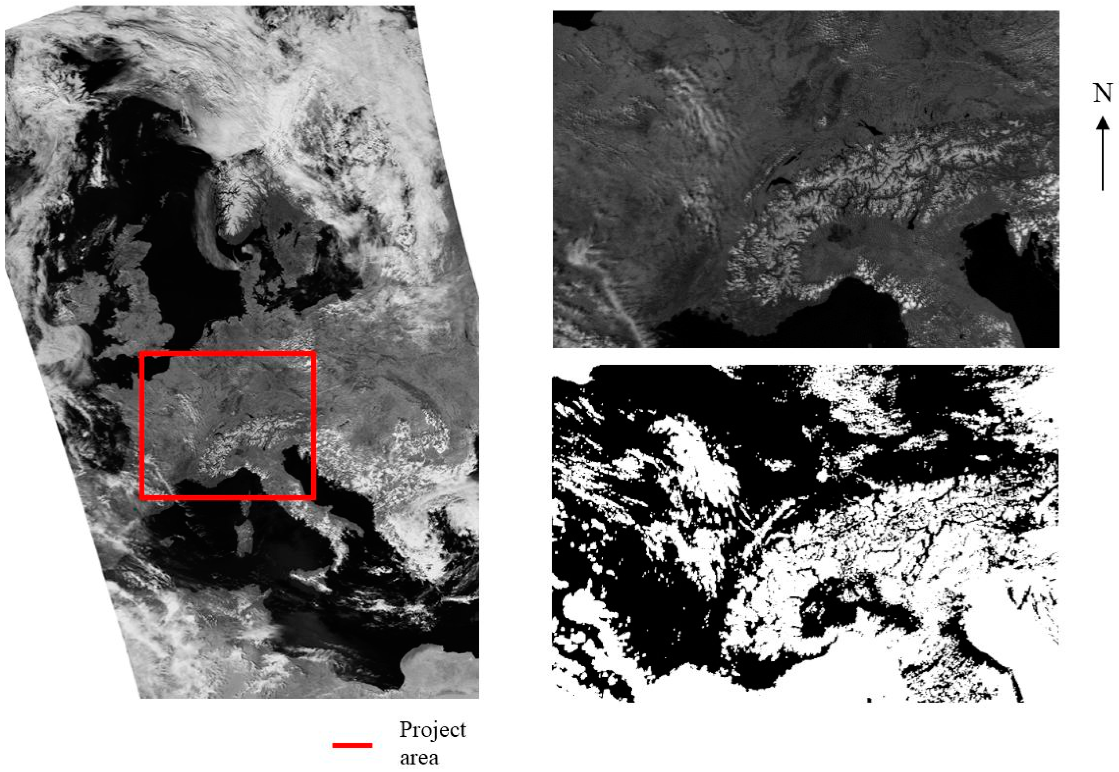
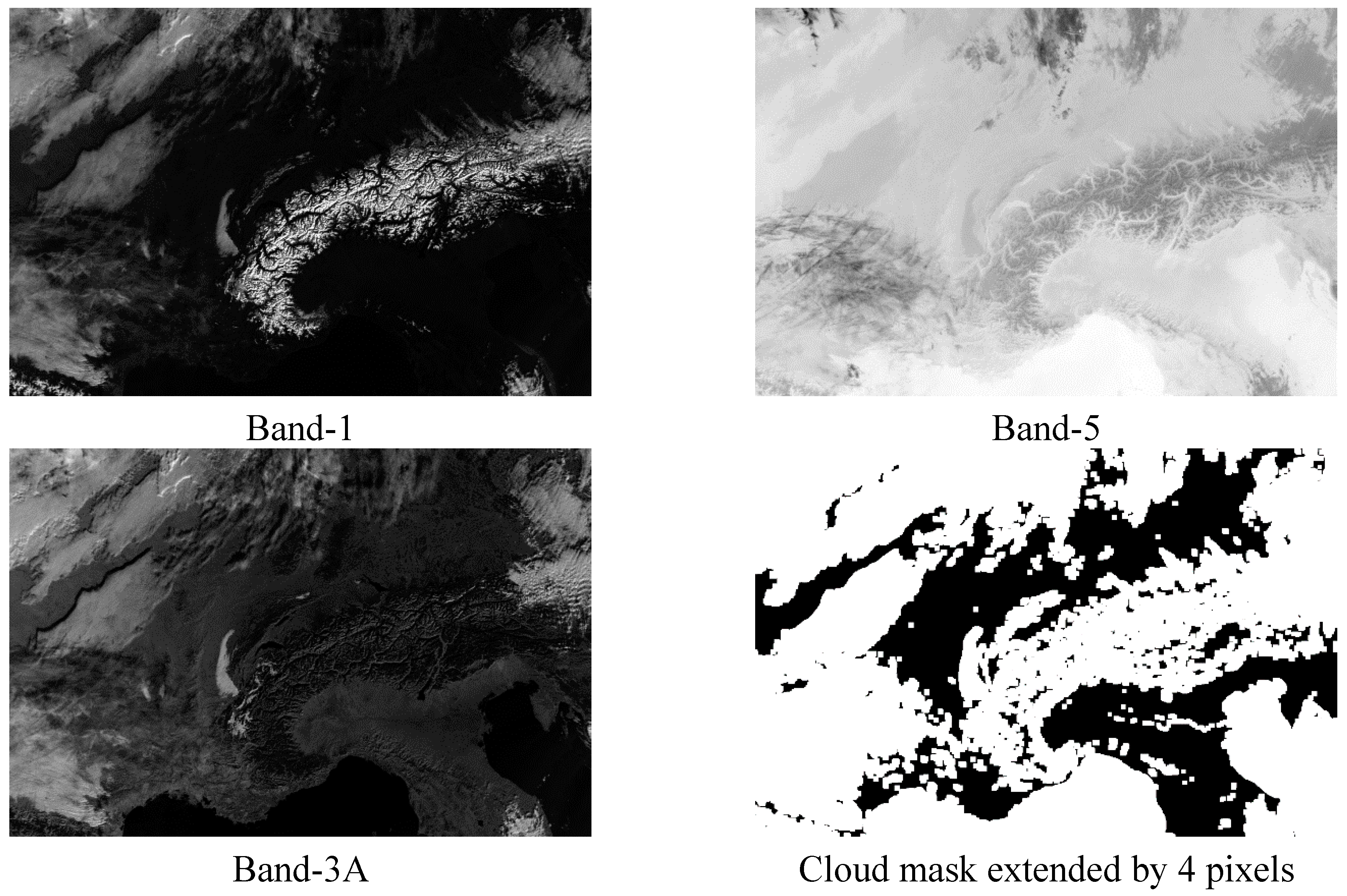
  • Extract cloud mask data (different masks for KLT tracking method and lake matching)
  • Crop both the image and the cloud mask data
These processing steps have also been implemented in Python with the help of OpenCV and Python imaging libraries [13,14]. Additional techniques have been applied to all images for the BBR accuracy investigations as explained in Section 2.3.

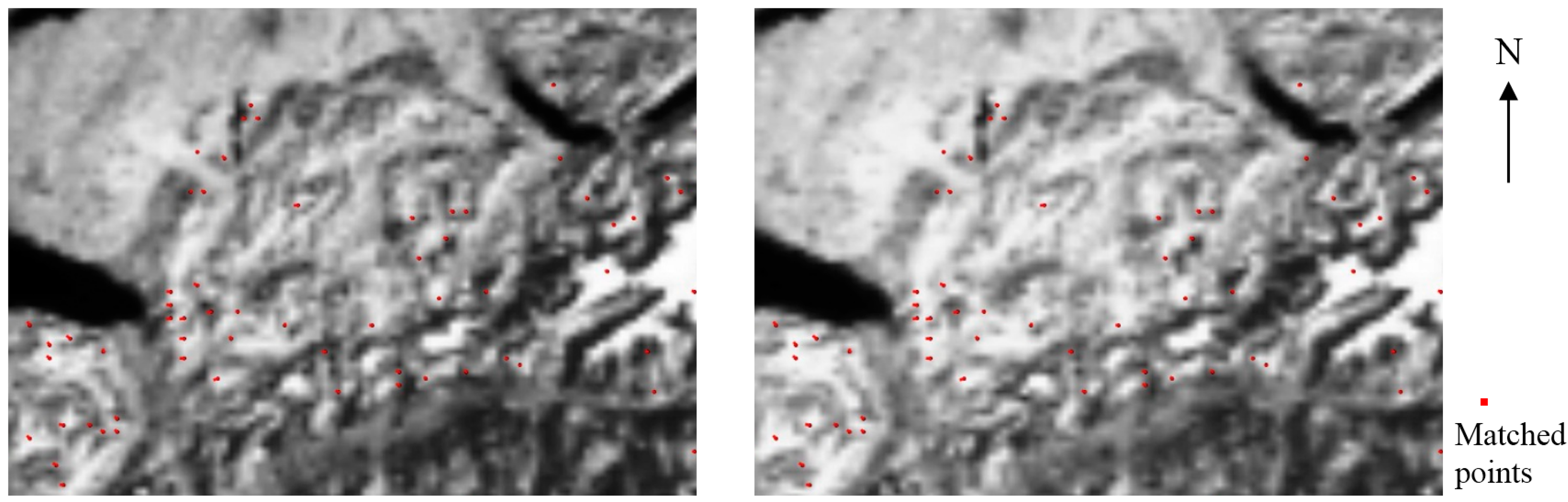
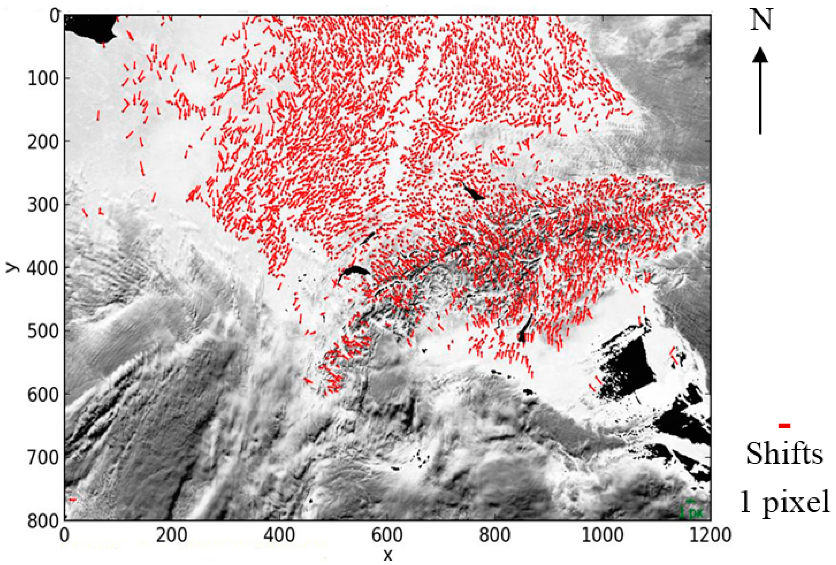
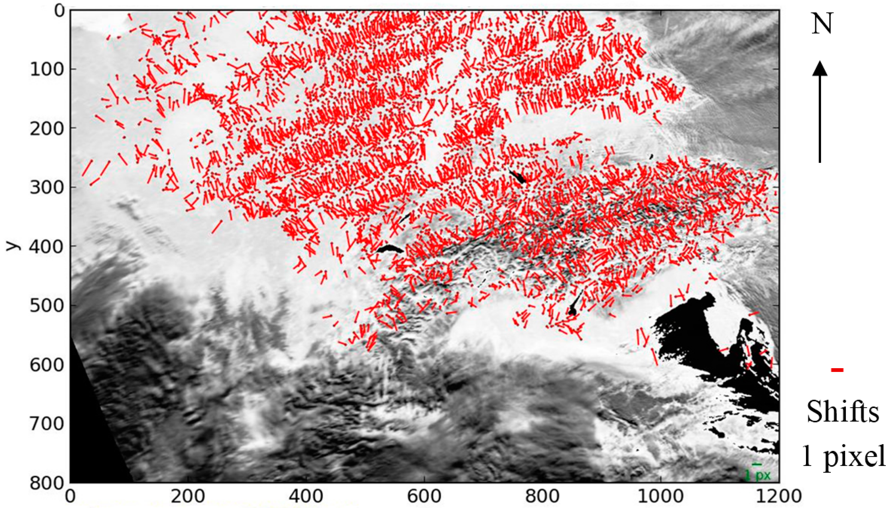
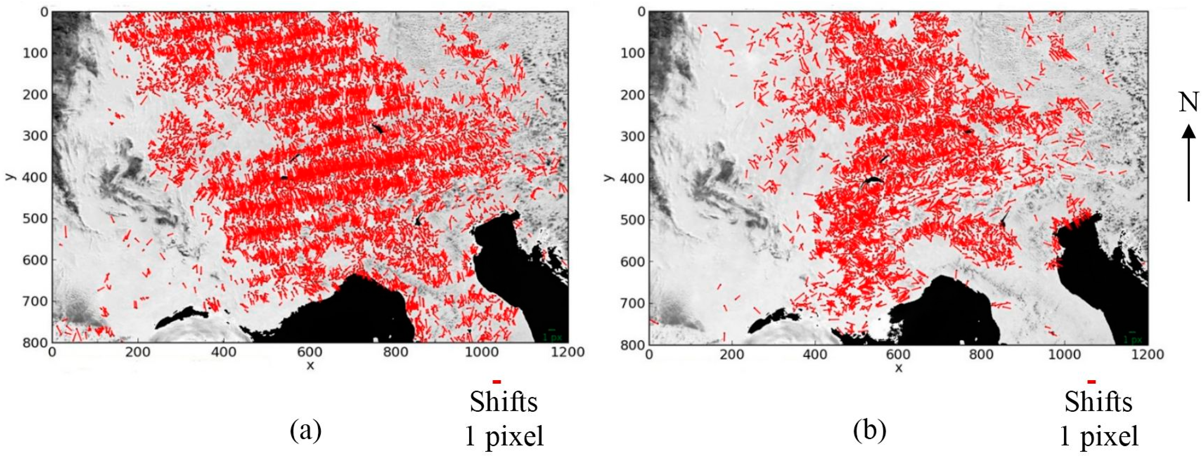
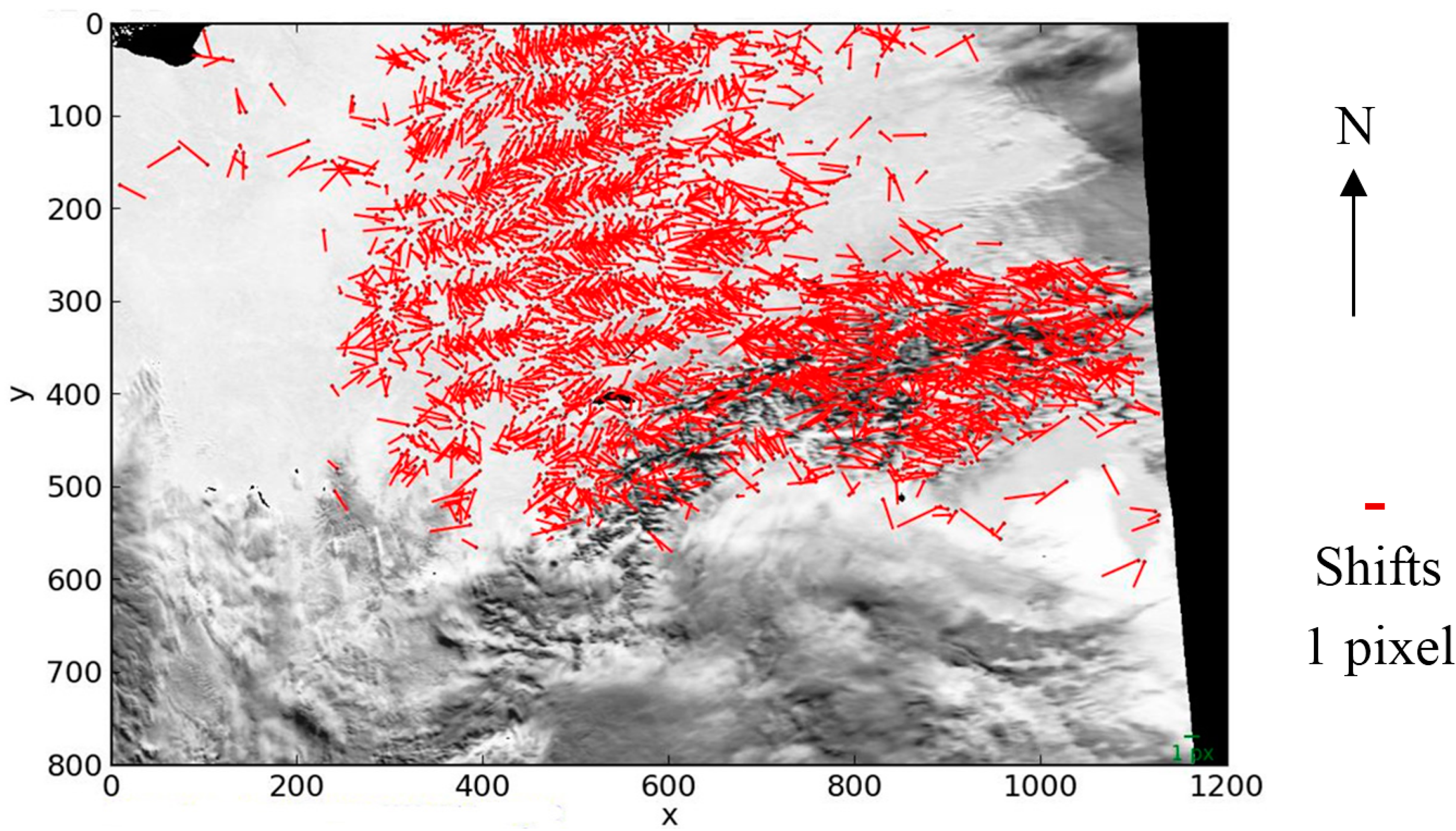
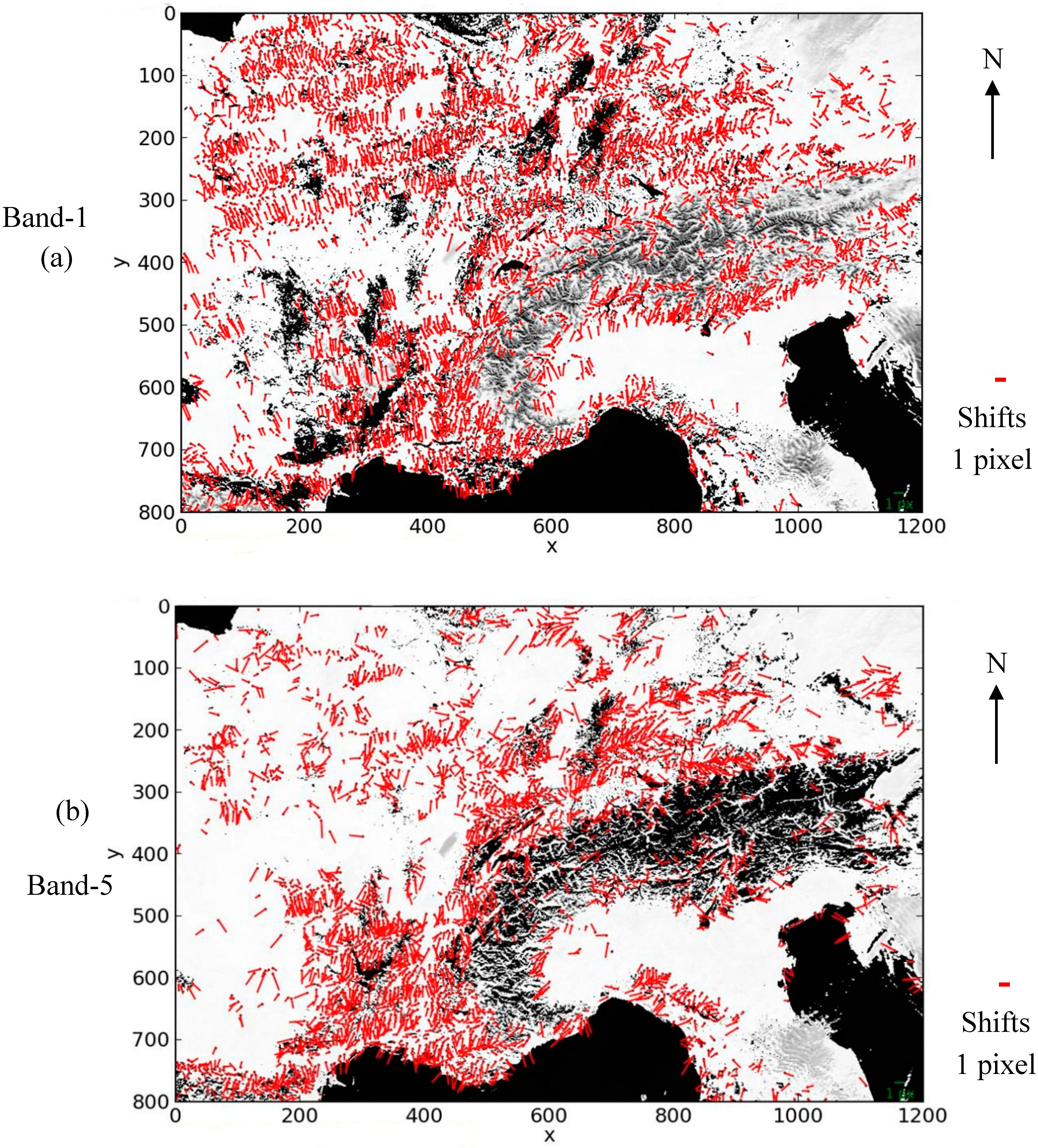
2.1. Relative Accuracy

The KLT tracking method has been used for matching of large numbers of image points between two images. A patch size of 15 × 15 pixels is used for matching. The relative accuracy has been investigated using the AVHRR Band-2 images of the same day. Figure 1 shows one full scene, its part used for the relative accuracy evaluation, and the corresponding cloud mask. The cloud mask used in the matching process with KLT tracking method includes: (a) clouds; (b) water; (c) cloud shadows over water, land, and snow; (d) pixels adjacent to cloud over water, land, and snow; and (e) no data (e.g., image borders with no information). The cloud masks of both images have also been combined for the matching of the pairs. Figure 2 shows parts from Band-2 images from two consecutive acquisitions from Metop-A and NOAA-17 on the same day. The points extracted from Metop-A images and successfully matched in NOAA-17 images are shown in both images. The average shift between the two images are 0.2 and 0.1 pixels in x and y, respectively, with standard deviations of 0.1 pixels in both directions.
Figure 1. AVHRR Band-2 orthoimage acquired from NOAA-18 on 7 May 2008 at 12:08 (left). The subarea used for relative accuracy tests is marked with red rectangle on the full image and shown in upper right image. The cloud mask used for relative accuracy tests is given in the lower right.
Remotesensing 07 03293 g001
Figure 2. AVHRR Band-2 orthoimages acquired on 10 July 2008 from Metop-A (left) at 09:36 and NOAA-17 (right) at 09:45. The matched points between the orthoimages are shown in both.
Remotesensing 07 03293 g002

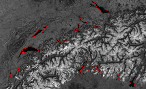
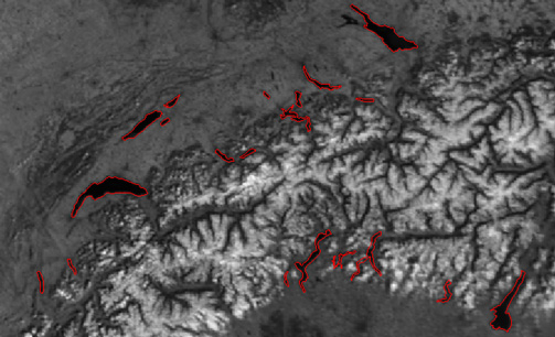
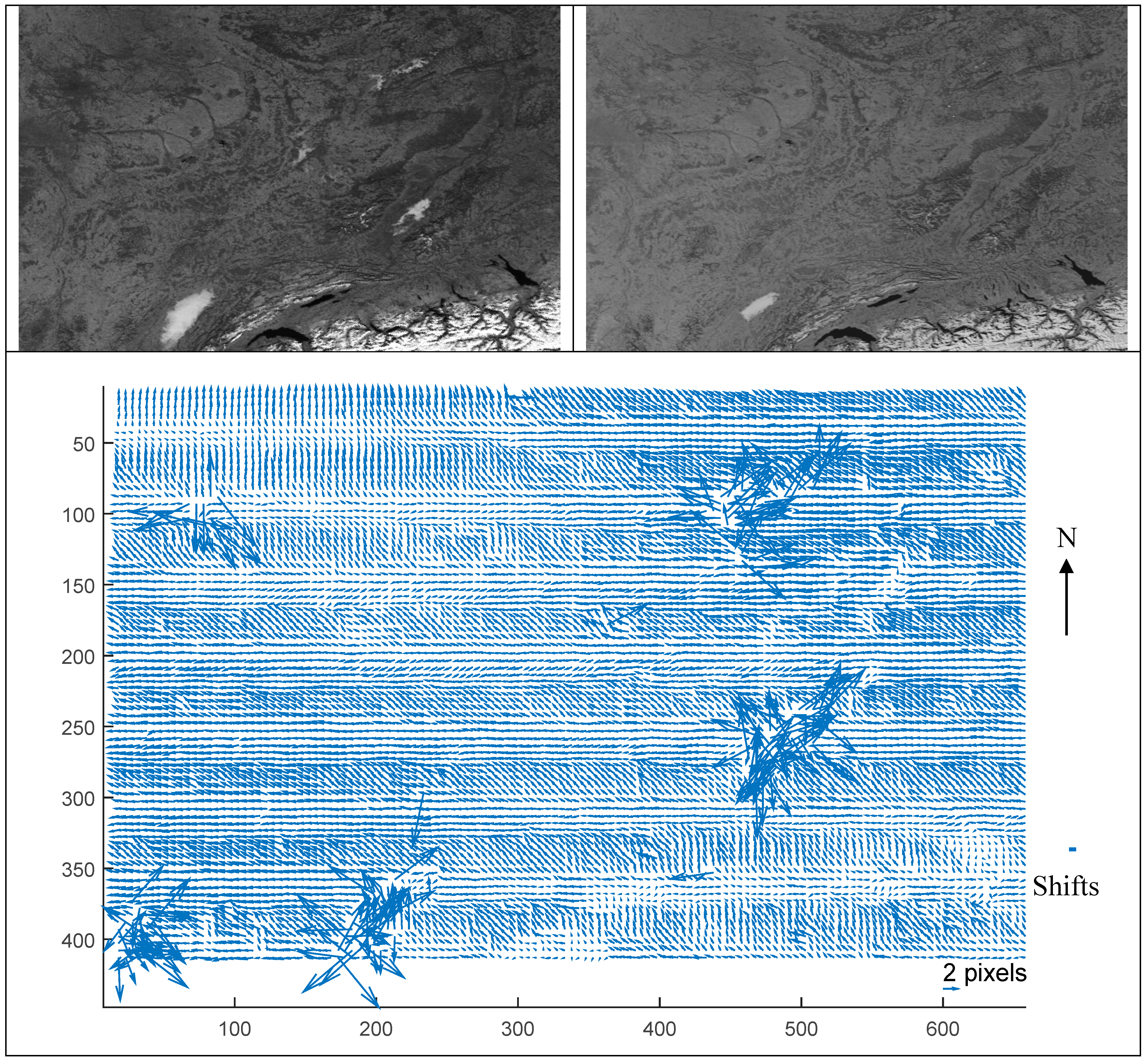
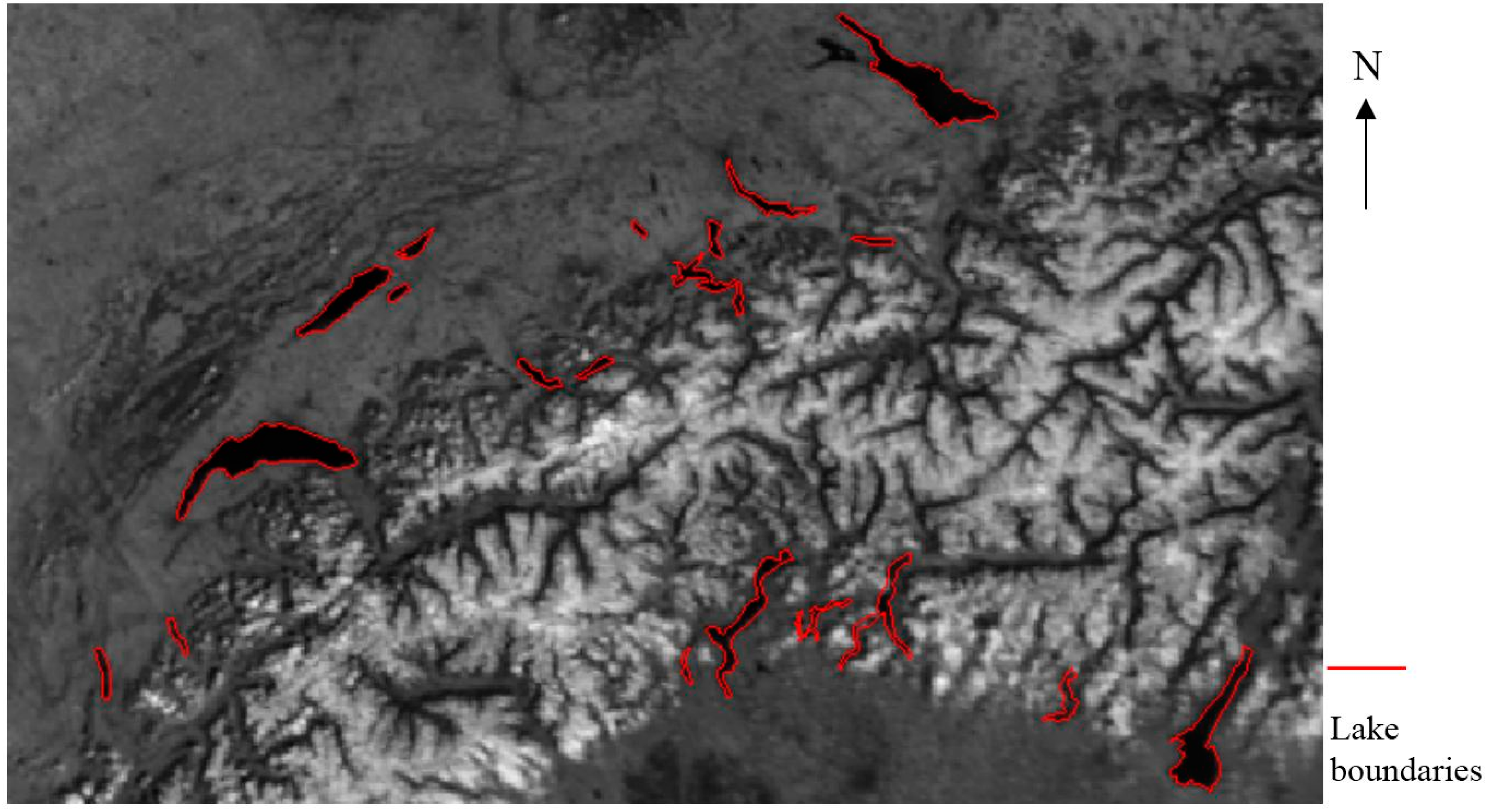
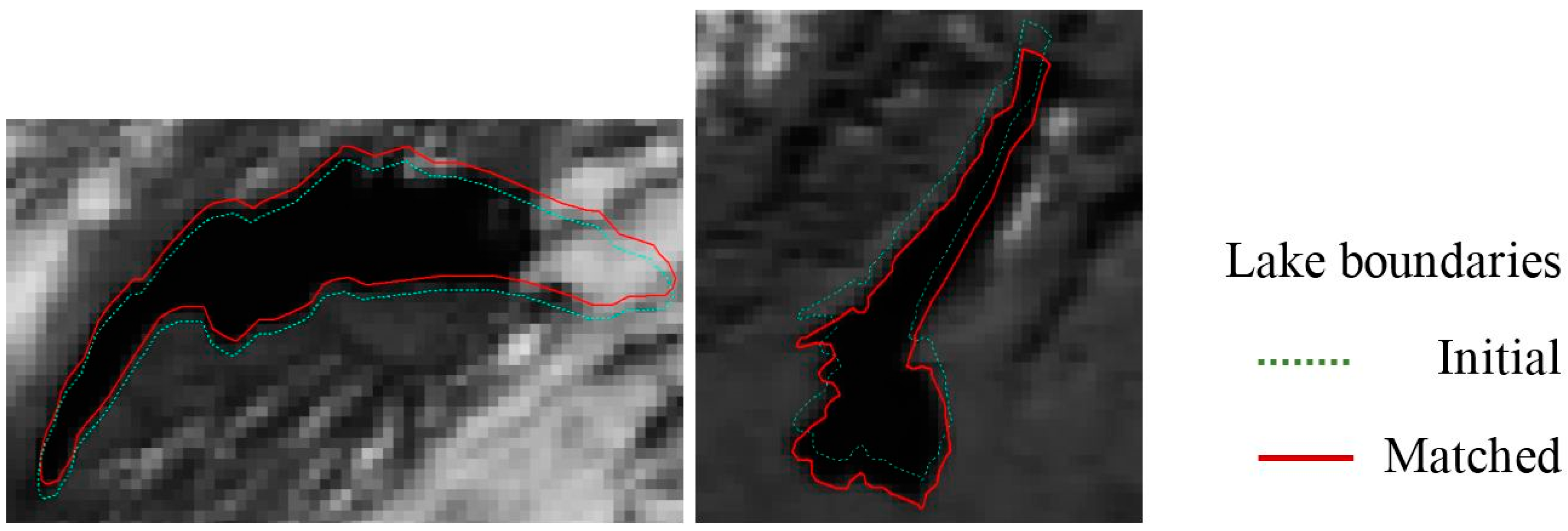
2.2. Absolute Accuracy

The absolute accuracy of the AVHRR imagery has been evaluated based on lakes by estimating the 2D shifts of the lake polygons in image space (i.e., orthoimage coordinate system). Band-2 was used, since lakes are dark in this band and demonstrate a good contrast compared to their surroundings. The evaluation is done based on lakes, since the detection of shorelines in the images is relatively easy and reliable [7]. In addition, with a resolution of 1 km, there are hardly any other stable image features in our test region that are well defined and measurable apart from lake and sea shorelines (and to a much lesser extent forest borders). An alternative would be to use orthorectified images of higher accuracy and resolution and match them with AVHRR orthoimages; however, this matching would be difficult due to large differences (spectral, multitemporal etc.) and was not feasible in this case. Each lake is matched in the images based on the minimization of normalized sum of pixel intensities inside the lake polygons [7]. A total of 20 lakes is used for the evaluations (Figure 3). The lakes were digitized from Landsat-5 orthoimages with 25 m resolution and their locations in the AVHRR images have been computed via coordinate transformations.
Regarding the cloud mask data, only no data and cloud pixels are used as mask in lake matching. Lakes having a cloud cover percentage over 60% are excluded from the process since the matching is usually not successful. The statistical parameters of the shifts are derived from all successfully matched lakes (equally weighted) within an image.

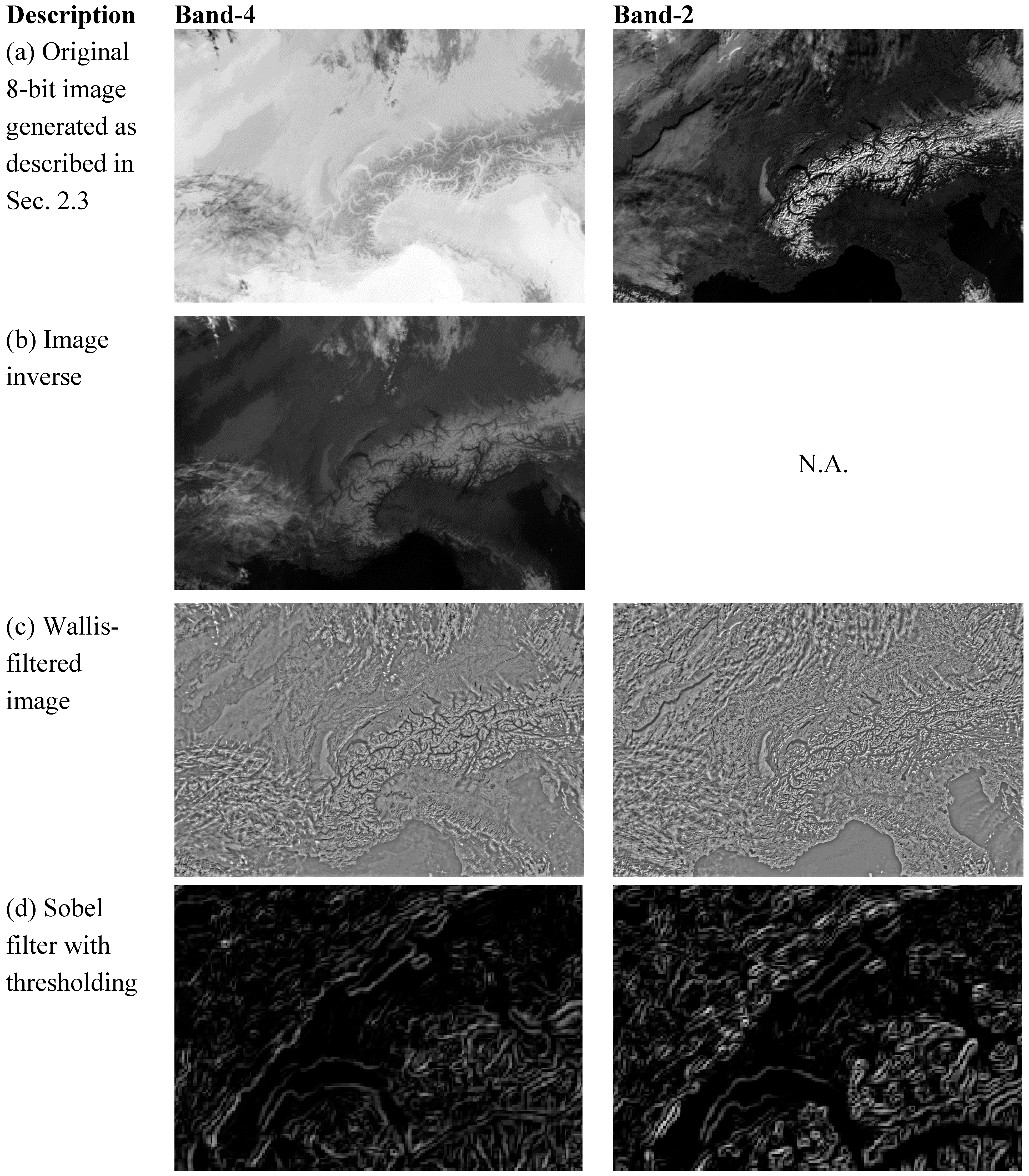
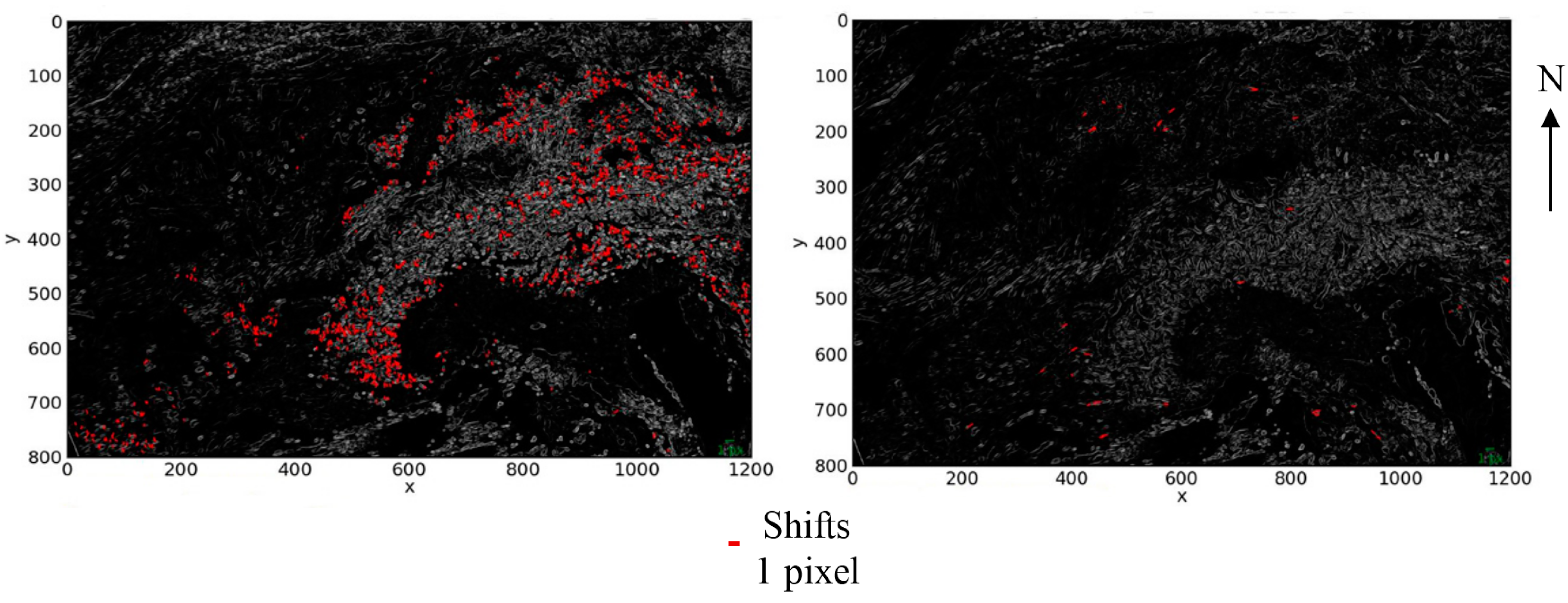
2.3. Band-to-Band Registration Accuracy

Band-to-band registration (BBR) accuracies of the six AVHRR bands are also evaluated using the KLT tracking method [12]. Band-2 images are used as reference for the other five bands (four bands per acquisition, since only 3A or 3B are transmitted to the ground). Band-2 was selected since it was used in the absolute accuracy and thus, through the BBR results, the absolute accuracy of all remaining bands could be determined. Due to large radiometric differences, the following preprocessing techniques are applied to the images prior to the matching:
  • Image inverse: Radiometric inverse has been applied to the Bands 3A, 3B, 4 and 5 since the appearance of the mountain areas are similar to those in Band-2 only after the inverse is taken. The functions in Python imaging library is used for this purpose [14].
  • Wallis filtering: applied to the image inverses to increase the local contrast and the radiometric similarity of the images. The method has been described in [15] and the software implementation has been done by the Photogrammetry and Remote Sensing Group at ETH Zurich. The same filtering parameters are used for all images (i.e., block size (20 × 20), target mean (127), target standard deviation (50), brightness enforcing constant (1), contrast enforcing constant (0.95)).
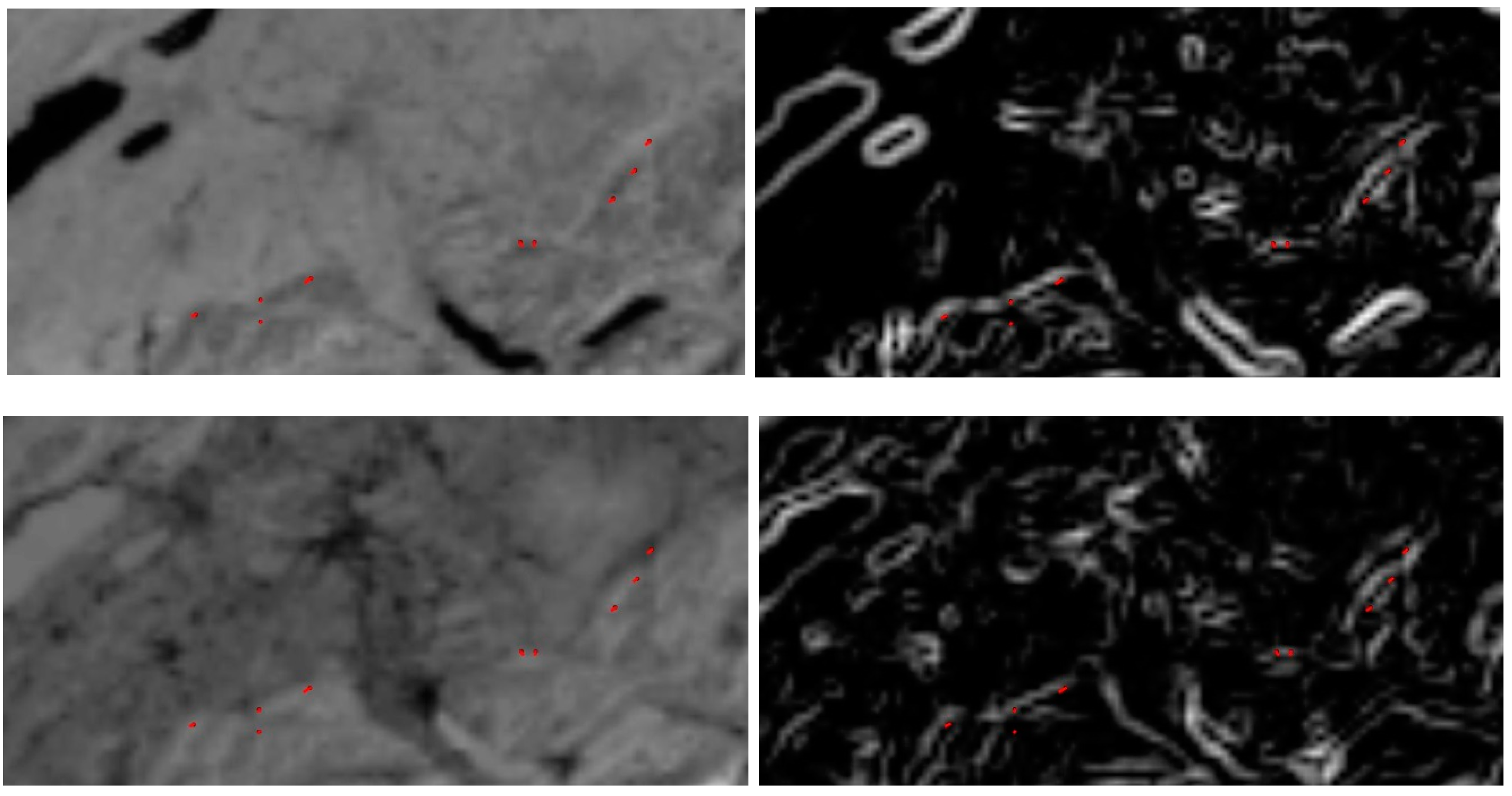
  • Sobel filtering: applied to the Wallis-filtered images to detect edges in the images. The filter has been implemented here using Python programming language.
  • Thresholding: reduces weak edges, often due to noise, from Sobel-filtered images. The threshold is selected as 50% of the cumulative histogram of edge gradients for all images.
Figure 3. AVHRR Band-2 image part acquired from Metop-A on 7 May 2008 at 10:00 and the lakes used for absolute accuracy investigations.
Remotesensing 07 03293 g003
After preliminary tests, a patch size of 9 × 9 pixels is selected as it led to the best matching results. The cloud masks, which have been used in relative accuracy evaluations and described above, have been expanded by 4 pixels (half the patch size) in order to prevent selection of candidate points close to cloud areas and thus reduce the matching errors caused by overlap of the matching patch with clouds. This problem was realized after the relative accuracy investigations. A stricter blunder detection, compared to relative accuracy, was also applied since correct matching of a smaller number of points (due to quasi-identical acquisition times and same orientation) would be sufficient to estimate band-misregistration errors, while the large spectral differences of the matched images caused more matching blunders, needing stricter detection. Figure 4 shows Band-2 and Band-4 images of one acquisition (from Metop-A on 23 January 2008) with all intermediate preprocessing steps applied prior to the matching (i.e., a: 8-bit image; b: inverse; c: Wallis filtered; d: Sobel filtered with thresholding). In the last one (Figure 4d), a smaller area is zoomed in, in order to provide better insight into the process. Figure 5 shows the remaining band images of the same acquisition together with the cloud mask.
Figure 6 shows parts from Band-2 and Band-5 images from Meteop-2 on 10 July 2008 at 09:36. The matching is performed on preprocessed (i.e., Wallis and Sobel filtered with thresholding) images. The candidate points were extracted from Band-2 images and matched in Band-5 images. The plots given in the Figure show the successfully matched points both on preprocessed images used for matching and also on original (linear stretched) images. The average shifts between the two images are 0.3 in both directions, with standard deviations of 0.3 and 0.1 pixels in x and y, respectively.
Figure 4. AVHRR Band-4 and Band-2 images acquired from Metop-A on 23 January 2008. (a) 8-bit image; (b) inverse ; (c) Wallis filtered; (d) Sobel filtered with thresholding.
Remotesensing 07 03293 g004
Figure 5. AVHRR Band-1, 5, and 3A images acquired from Metop-A on 23 January 2008 and the cloud mask used in the matching.
Remotesensing 07 03293 g005
Figure 6. Parts of AVHRR Band-2 (top) and Band-5 (bottom) images acquired on 10 July 2008 at 09:36 from Metop-A. The matched points between the preprocessed images (right) are shown in both and presented on linear stretched images (left) as well.
Remotesensing 07 03293 g006

3. Results and Discussion

The relative and absolute accuracy have been investigated using the AVHRR Band-2 images from 24 different days in 2008. For the relative accuracy evaluations, only the images acquired on the same day have been matched. Up to five acquisitions from all three sensors per day are available. However, due to the inferior GSD of the large off-nadir images, only three images, which cover Switzerland at nadir or near-nadir position, have been used. On the other hand, a total of four images for some days has been evaluated when two images taken from the same sensor have similar off-nadir angles.
Since systematic errors have been observed during the relative accuracy tests (see Section 3.1.2), further analysis has been performed using additional data: i.e., all spectral bands for some days, images processed with two orthoimage generation software versions (SAPS v. 2.0 and 3.0), data of one day in 2009 including images from NOAA-19, and matching original Level 1B reflective images. The data used for these tests are described in the corresponding sections below.

3.1. Relative Accuracy Results

3.1.1. Results (Overall)

A total of 75 images from 24 days was used for matching. The images acquired on the same day from different sensors are matched by pairing the images with shorter time interval in order to reduce matching errors caused by illumination and cloud differences. For example, on the 23 January, three images acquired from Metop-A at 09:33, from NOAA-17 at 09:59, and from NOAA-18 at 11:56 are matched by pairing Metop-A-NOAA-17 and NOAA-17-NOAA-18 images. The matching results of a total of 51 image pairs are given in Table 2 separately for different satellite combinations. P0 and P1 denote the number of candidate and matched points. The Min, Max, Mean, Median (MED), and the standard deviation (σ) values in the second column (Parameter) are derived from all image pairs obtained from the respective satellites given in the first column. The Shift (x, y), MED (x, y), σ(x, y) and MAD(x, y) values are computed from all successfully matched points in an image pair. The Shift, MED, σ and MAD values are presented in the table as absolute shifts (not signed). In this table, only absolute values have been presented to highlight the magnitude of the errors, while with signed shifts the signed mean could be small although the individual shifts large. The Max shifts obtained from the matching of Metop-A and NOAA-17 images are 1.8 (x) and 2.9 (y) pixels. Between the Metop-A-NOAA-18 images, the Max shifts are 1.1 (x) and 0.9 (y) pixels. Between NOAA-17-NOAA-18, the Max shifts are 1.6 (x) and 0.6 (y) pixels. Two NOAA-18 pairs are also evaluated and the Max shifts are 1.1 (x) and 0.1 (y) pixels.
The differences between P0 and P1 are caused by the matching error elimination strategy based on the statistical evaluation (see Section 2). The σ values obtained in the matching are higher than those previously obtained from MSG-SEVIRI images. This can be explained by the larger illumination and atmospheric differences between the images (longer image acquisition intervals), matching images of different satellite sensors and different viewing angles, and existence of local systematic errors in the images. As explained in the next section, systematic errors in stripe layout are observed in all NOAA-18 images.
Figure 7 and Figure 8 (split in two due to space constraints) show the mean x-, y-shifts for all pairs. It can be seen in Figure 8 that the larger shifts occurred after August 2008 on some days only, involving pairs of all three satellites. The green dotted lines in Figure 8 denote the range of vertical axis of Figure 7 for comparison.
Table 2. Relative accuracy evaluation; statistical values of shifts (x) and (y) from 51 image pairs acquired on 24 different days in 2008. All results except the number of points P0 and P1 are given in pixels and are derived from absolute values.
SatellitesParameterP0P1Shift (x)Shift (y)σ (x)σ (y)MED (x)MED (y)MAD (x)MAD (y)
Metop-A & NOAA-17
(25 pairs)
Min149011730.00.00.10.10.00.00.10.1
Max500044551.82.91.01.21.72.90.60.9
Mean462337010.40.40.40.40.30.40.30.3
MED500039600.20.20.40.30.20.20.20.2
σ8447330.50.70.20.30.40.70.10.2
Metop-A & NOAA-18
(9 pairs)
Min284819790.00.00.30.50.10.10.20.4
Max500044271.10.90.81.01.10.70.50.7
Mean469836320.20.30.50.60.20.20.30.5
MED500038140.10.20.40.50.10.20.30.4
σ7188340.30.20.20.20.30.20.10.1
NOAA-17 & NOAA-18
(15 pairs)
Min15353720.00.00.30.50.00.00.20.3
Max500046511.60.61.00.71.60.50.60.5
Mean443729380.30.20.50.50.30.20.30.4
MED500030930.10.20.50.50.20.20.30.4
σ100510970.40.10.20.10.40.10.10.0
NOAA-18 & NOAA-18
(2 pairs)
Min398925580.70.00.80.70.60.00.40.5
Max500031791.10.11.40.91.10.10.70.6
Mean449528690.90.11.10.80.80.10.60.5
MED449528690.90.11.10.80.80.10.60.5
σ7154390.30.10.40.10.30.10.20.0
Figure 7. The mean x-, y-shifts obtained from 32 image pairs obtained from Metop-A, NOAA-17 and NOAA-18 between January and August 2008. Horizontal axis: Time, Vertical axis: pixels.
Remotesensing 07 03293 g007
Figure 8. The mean x-, y-shifts obtained from 19 image pairs obtained from Metop-A, NOAA-17 and NOAA-18 between September and December 2008. Horizontal axis: Time, Vertical axis: pixels.
Remotesensing 07 03293 g008

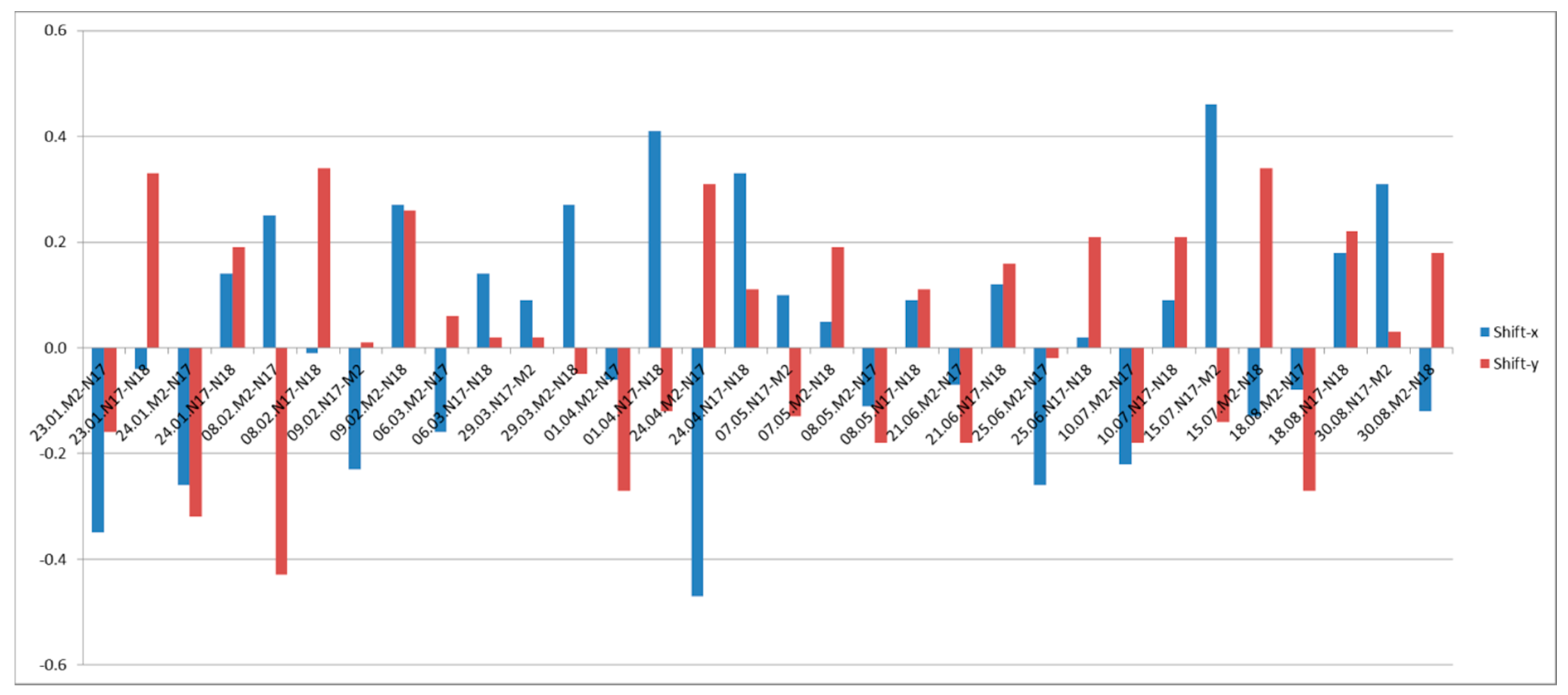
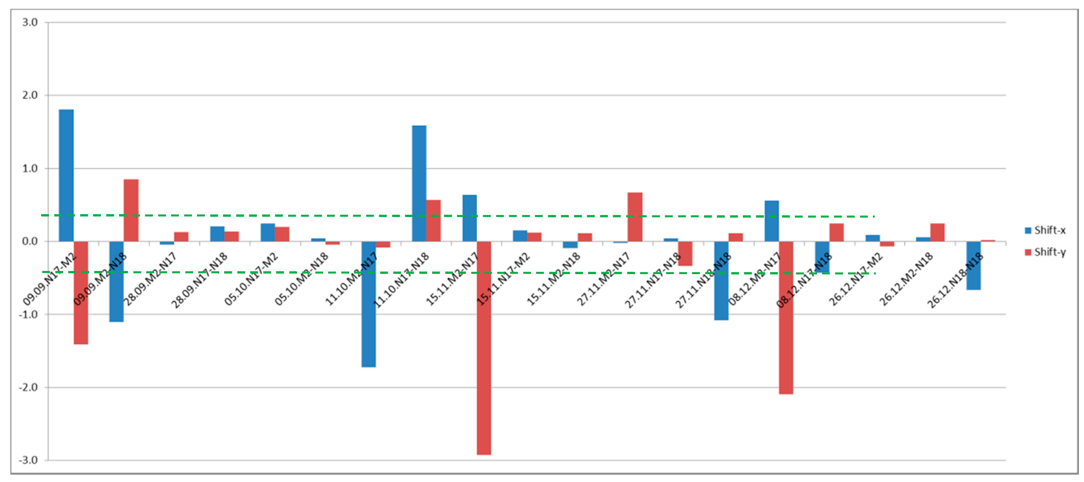
3.1.2. Systematic Errors

During the relative accuracy tests, systematic stripes have been observed in some of the image pairs. After visual inspections on the shift plots of all 51 pairs, it has been seen that this effect exists in all pairs where NOAA-18 images are involved (i.e., Metop-A/NOAA-18, NOAA-17/NOAA-18, and NOAA-18/NOAA-18 pairs). These systematic errors have been investigated further using additional data as mentioned before Section 3.1.1.
Figure 9, Figure 10 and Figure 11 show the shift plots of three image pairs acquired on 26 December 2008. In the figures of this Section, the vectors are not shown with background of the original images, since the vectors would be hardly visible, but on images that were especially preprocessed to suppress the background, keeping water surfaces dark for better visualization (thus, what appears in the background as being clouds, is not really so). In Figure 10, the image pair, which contains NOAA-18 image, shows systematic errors as stripes across the flight direction of NOAA-18. This sort of systematic errors can be seen also in the matching of two NOAA-18 images from the same day (Figure 11), but due to phase differences the stripes may appear differently. Stripes have also been observed along the whole length of an AVHRR image (in N. Europe and N. Africa).
The striping errors occur for NOAA-18 and for NOAA-19 (for the latter only one day in 2009 has been checked). Both satellites take images while ascending, however no reason could been seen why ascending image acquisition should have such systematic errors. The stripes are perpendicular to the satellite track and alternating with a width of about 30 pixels (corresponding to 5 s of data acquisition), i.e., one stripe has shifts of about 1 pixel in flight direction, the next stripe has no shifts, etc. The stripes appear in all spectral bands. The matched images were from the same day and using the same DSM as input to the orthorectification. Although the GCPs were different for the various AVHRR images, their number and distribution were quite similar for the same day, with differences mainly due to varying clouds and less illumination. The stripes appear over the whole length of the original AVHRR images (from Scandinavia to N. Africa). This investigation has been done since in the AVHRR orientation with SAPS, the image is divided into three almost equal segments, and orientation errors may differ for each segment. They also have a very high frequency, which cannot be explained by errors in sensor orientation or DSM. The error is assumed to be existing in the input data for orthorectification (Level 1B), due perhaps to errors of geometric calibration, scanning or time synchronization between the system’s position and attitude determination units. An additional indication that the systematic errors exist in the Level 1B data is the inclination of the stripes (see Figure 10, Figure 11, Figure 12 and Figure 13). The stripe direction (long dimension) is not aligned with North/South used in the orthoimage generation but is perpendicular to the flight direction of ascending NOAA-18/19 satellites. Thus, the Level 1B images have also been checked.
Figure 9. Image space shifts obtained from matching of NOAA-17 and Metop-A images acquired on 26 December 2008. The axes denote the image coordinates.
Remotesensing 07 03293 g009
Figure 10. Image space shifts obtained from matching of Metop-A and NOAA-18 images acquired on 26 December 2008. The axes denote the image coordinates.
Remotesensing 07 03293 g010
Figure 11. Image space shifts obtained from matching of two NOAA-18 images acquired on 26 December 2008. The axes denote the image coordinates.
Remotesensing 07 03293 g011
Additional data acquired on 6 August 2009 has been provided by the University of Bern, where one acquisition from NOAA-19 satellite is also included. Similar striping errors in across-track direction are also observed in the NOAA-19 image. The shift plots from the matching of NOAA-17 and NOAA-18 images with the NOAA-19 image are provided in Figure 12a,b.
Figure 12. Image space shifts obtained from matching of NOAA-18-NOAA-19 (a) and NOAA-17-NOAA-19 (b) images acquired on 6 August 2009. The axes denote the image coordinates.
Remotesensing 07 03293 g012
The analysis of NOAA-18 images has been extended by using the bands for the some days. As can be seen in the Figure 13a,b, the stripes are clearly visible in the matching of two different bands (Band-1 and Band-5) acquired on 8 February 2008.
Figure 13. Image space shifts obtained from the matching of the Band-1 (a) and Band-5 (b) images acquired from NOAA-17 and NOAA-18 on February 8, 2008. The axes denote the image coordinates.
Remotesensing 07 03293 g013
All data were generated by SAPS v. 2.0. We also processed some data generated by SAPS v3.0 and the results were practically identical. To reduce the risk that the systematic stripe problem was due to a software problem, the University of Bern analysed all outputs of the SAPS processing software and checked the quality of the georeferencing and matching between MODIS and AVHRR. No problem could be detected, even using different versions of the SAPS software. The author of SAPS was also informed about this systematic error but could not provide any explanation (Khlopenkov, personal communications). Furthermore, A.P. Cracknell (personal communications) who has worked extensively with AVHRR was contacted for a possible explanation of the systematic stripes, but he could not provide one.
Figure 14. Matching of Band-2 L1B images (input to orthorectification). Top: left NOAA-17 after being co-registered with NOAA-18, right NOAA-18. Bottom: shifts after matching NOAA-17 with NOAA-18. The large vectors correspond to matching errors due to multitemporal differences (e.g., clouds) and significant other differences in grey values due to different illumination conditions, viewing angle, etc. The systematic stripes are clearly visible. They have a width of about 30 pixels, and alternating shifts of about 1 and 0 pixels. The axes in the plot (bottom) denote the image coordinates.
Remotesensing 07 03293 g014
Original Level-1B AVHRR reflective images (radiometrically calibrated) have also been used to find out if the systematic errors exist also in the original images. After the finalization of this project, we used accurate coregistration methods to perform the matching between L1B images within another project [16]. These methods computed a co-registration with 3rd degree polynomial (20 parameters) between NOAA-17 and NOAA-18 images by using about 350 hundred points found and matched with SIFT, and manually edited to exclude blunders. As can be seen in Figure 14, the systematic stripes are visible in the results. The matching between the transformed NOAA-17 and the original NOAA-18 image are dense on a regular grid, instead of using good texture points as with KLT; thus, the systematic pattern is more visible. The matching algorithm used between the co-registered images was a Fourier-Transform based Cross-Correlation (FTCC) as explained in [16]. Thus, we can show that this error exists in the L1B data and is not due to the orthorectification software. This error maybe due to errors of calibration, scanning or time synchronization between the system’s main three units. We will do further future investigations and contact experts of the NOAA-18 sensors to try to find the cause.

3.2. Absolute Accuracy Results

A total of 72 images acquired on 23 different days (one day excluded due to total cloud coverage) has been processed using lake matching. Figure 15 shows the plots of two lake polygons at their initial and the matched positions in the images. The results are summarized in Table 3, Table 4 and Table 5 for Metop-A, NOAA-17 and NOAA-18. The shifts in Table 3, Table 4 and Table 5 show that up to 4 pixels, 1.6 pixels and 1 pixel shifts are present in Metop-A, NOAA-17 and NOAA-18 images, respectively. The shifts are shown with signs, where +Δy indicates a shift to the North and +Δx indicates a shift to the East.
Figure 15. Lake matching results from Lake Leman in a NOAA-17 image (left) and Lake Garda in a Metop-A image (right). The green polygons represent the initial positions of the lake points and the red polygons represent the matched positions.
Remotesensing 07 03293 g015
The standard deviations (σx, σy) given for each date show the variability in the shifts of all lakes in an image. The larger standard deviations, which occurred in the shifts of all lakes within an image, have been observed in the more off-nadir images. The standard deviations increase even more (up to 0.7 pixels) at the off-nadir images, which are excluded from the analysis in the following tables (images closer to the nadir are preferred for each day). However, in each table, there are days with two acquisitions, where both images were acquired from a relatively off-nadir position.
When the mean and σ values (given in the lower part of the Tables) of Shift (x) and Shift (y) parameters are compared for all three satellites, it can be said that NOAA-17 and NOAA-18 images have better absolute accuracy than Metop-A. The mean (x,y) shifts obtained from all 24 images of NOAA-17 are (0.2, −0.2) pixels with shift standard deviations of (0.3, 0.2) pixels. For NOAA-18, the mean (x, y) shifts are (0.1, −0.3) pixels with standard deviations of (0.2, 0.2) pixels. For Metop-A images, although the mean (x, y) shifts are small (−0.1, −0.4 pixels), the standard deviations of shifts are high (0.4, 1.1 pixels), which reflects existence of large shifts, especially in y, on three days. The results of these days were visually checked, but no matching errors could be found.
Table 3. Absolute accuracy evaluation; statistical summary from the lake shifts (equally weighted) in AVHRR images acquired from Metop-A. All values are in pixels except the number of lakes and are derived from signed values.
DateShift (x)Shift (y)σ (x)σ (y)MED (x)MED (y)MAD (x)MAD (y)No. of Lakes
23.01.2008−0.4−0.30.20.3−0.5−0.30.20.220
24.01.2008−0.1−0.80.30.3−0.2−0.80.20.220
08.02.2008−0.2−0.60.20.2−0.2−0.60.20.220
09.02.2008−0.4−1.50.30.3−0.4−1.60.30.220
09.02.20080.3−0.10.30.40.4−0.10.30.320
06.03.2008−0.1−0.20.20.3−0.1−0.20.20.220
29.03.20080.2−0.40.20.30.2−0.50.10.318
01.04.20080.0−0.40.10.10.0−0.40.10.17
07.05.20080.10.00.20.20.00.00.10.120
08.05.20080.0−0.30.10.10.0−0.30.10.119
21.06.20080.0−0.20.20.20.0−0.20.10.020
25.06.2008−0.1−0.10.10.1−0.1−0.10.10.119
10.07.20080.0−0.10.20.20.0−0.10.10.119
15.07.2008−0.20.40.10.3−0.20.40.10.220
18.08.20080.0−0.20.20.20.0−0.30.10.119
30.08.2008−0.1−0.10.40.3−0.1−0.10.20.216
09.09.2008−1.72.00.40.5−1.61.80.30.320
28.09.20080.1−0.10.40.40.2−0.10.20.314
05.10.20080.0−0.40.20.20.0−0.40.10.220
11.10.2008−0.30.00.20.3−0.30.00.10.211
15.11.20080.4−4.00.40.40.5−4.20.30.211
27.11.2008−0.40.10.20.4−0.40.10.20.314
08.12.20080.3−2.30.30.40.3−2.40.20.413
26.12.20080.0−0.40.30.30.0−0.50.20.318
Min−1.7−4.00.10.1−1.6−4.20.10.07
Max0.42.00.40.50.51.80.30.420
Mean−0.1−0.40.20.3−0.1−0.50.20.217.4
MED0.0−0.20.20.30.0−0.30.20.219.0
σ0.41.10.10.10.41.10.10.13.7
Table 4. Absolute accuracy evaluation; statistical summary from the lake shifts in AVHRR images acquired from NOAA-17. All values are in pixels except the number of lakes and are derived from signed values.
DateShift (x)Shift (y)σ (x)σ (y)MED (x)MED (y)MAD (x)MAD (y)No. of Lakes
23.01.20080.0−0.20.20.30.0−0.20.20.320
24.01.20080.2−0.40.20.20.2−0.50.10.320
08.02.2008−0.30.00.20.3−0.3−0.10.10.320
09.02.20080.0−0.30.20.20.0−0.30.10.220
06.03.20080.1−0.20.20.20.1−0.20.10.219
29.03.20080.4−0.10.20.20.3−0.20.10.118
01.04.20080.0−0.20.10.20.0−0.30.10.19
07.05.20080.2−0.10.20.30.2−0.20.10.120
08.05.2008−0.1−0.20.40.4−0.3−0.30.30.219
08.05.20080.1−0.20.40.40.1−0.10.20.319
21.06.20080.20.10.30.20.20.00.20.117
25.06.20080.20.00.20.10.30.00.10.019
10.07.20080.10.00.20.20.10.00.10.220
15.07.20080.20.00.20.20.30.10.10.120
18.08.20080.0−0.10.20.10.10.00.10.120
30.08.20080.1−0.10.20.10.00.00.10.117
09.09.20080.0−0.20.10.20.0−0.20.10.120
28.09.20080.3−0.20.50.30.4−0.10.20.215
05.10.20080.3−0.20.20.20.2−0.20.10.219
11.10.20081.60.30.40.31.60.30.30.212
15.11.20080.2−0.60.30.40.2−0.60.20.313
27.11.2008−0.2−0.60.30.3−0.2−0.60.20.412
08.12.20080.0−0.30.30.3−0.1−0.30.10.313
26.12.20080.1−0.40.30.30.1−0.40.10.318
Min−0.3−0.60.10.1−0.3−0.60.10.09
Max1.60.30.50.41.60.30.30.420
Mean0.2−0.20.30.20.1−0.20.10.217.5
MED0.1−0.20.20.20.1−0.20.10.219.0
σ0.30.20.10.10.40.20.10.13.3
Table 5. Absolute accuracy evaluation; statistical summary from the lake shifts in AVHRR images acquired from NOAA-18. All values are in pixels except the number of lakes and are derived from signed values.
DateShift (x)Shift (y)σ (x)σ (y)MED (x)MED (y)MAD (x)MAD (y)No. of Lakes
23.01.20080.1−0.60.20.50.2−0.60.20.517
24.01.20080.2−0.50.30.50.3−0.80.20.116
08.02.2008−0.2−0.50.20.3−0.2−0.50.20.220
09.02.20080.0−0.60.20.30.1−0.60.10.320
06.03.20080.1−0.20.20.40.1−0.10.20.218
29.03.20080.1−0.40.20.30.1−0.40.10.220
01.04.2008−0.10.10.40.30.00.10.20.39
07.05.20080.0−0.10.20.30.0−0.10.20.217
08.05.20080.1−0.20.30.20.2−0.20.10.119
21.06.20080.2−0.10.20.30.2−0.10.10.218
25.06.20080.2−0.20.20.30.3−0.30.20.312
10.07.20080.2−0.10.20.30.30.00.10.220
15.07.20080.0−0.40.30.5−0.1−0.70.20.220
18.08.20080.1−0.10.20.40.1−0.10.10.419
30.08.20080.2−0.20.20.40.2−0.20.10.319
09.09.20080.2−0.20.20.30.2−0.10.10.217
28.09.20080.1−0.20.10.30.1−0.20.10.217
05.10.20080.3−0.20.20.30.3−0.30.10.28
11.10.20080.3−0.60.30.40.4−0.60.20.112
15.11.20080.0−1.00.30.40.0−1.10.20.314
27.11.20080.0−0.30.40.30.0−0.30.20.317
08.12.20080.1−0.40.20.50.0−0.50.10.313
08.12.20080.7−0.70.30.30.6−0.70.20.316
26.12.20080.0−0.50.40.5−0.1−0.70.30.120
Min−0.2−1.00.10.2−0.2−1.10.10.18
Max0.70.10.40.50.60.10.30.520
Mean0.1−0.30.20.40.1−0.40.10.216.6
MED0.1−0.30.20.30.1−0.30.20.217.0
σ0.20.20.10.10.20.30.10.13.5

3.3. BBR Accuracy Results

The images of 63 acquisitions from 24 different days have been processed for the BBR accuracy analysis. The plots of the shift vectors for two different bands of the NOAA-18 acquisition on 27 November 2008 are given in Figure 16. The matching results are provided in Table 6, Table 7, Table 8, Table 9 and Table 10, one per band, and given separately per satellite. P0 and P1 indicate the numbers of the candidate and the matched points. These values are in general much lower than for the relative accuracy investigations, due to matching difficulties and mainly stricter blunder detection criteria (thresholds). Given that the same georeferencing parameters and DSM are used for all bands, the test results provided here should represent the BBR accuracy of the original bands plus the accuracy of matching, the latter having its influence even if matching the original images. The Shift, MED, σ and MAD values are computed using the absolute shifts (not signed).
As can be seen in Table 6, the mean (x,y) shifts are (0.07, 0.03) pixels for Metop-A, (0.04, 0.03) pixels for NOAA-17 and (0.08, 0.09) pixels for NOAA-18 between Bands 1 and 2. The maximum (x,y) shifts are (0.12, 0.08) pixels for Metop-A, (0.11, 0.12) pixels for NOAA-17 and (0.15, 0.21) pixels for NOAA-18. For Band-3A (Table 7), the mean (x, y) shifts are (0.17, 0.05) pixels for Metop-A and (0.15, 0.04) pixels for NOAA-17. The maximum (x, y) shifts are (0.28, 0.14) pixels for Metop-A and (0.35, 0.10) pixels for NOAA-17. For Band-3B (Table 8), only the data from NOAA-18 is available in the given dataset. It can be seen that the mean x-shift is comparable to those of Band-3A (0.16 pixels). The mean y-shift is slightly higher (0.13 pixels) than that of Band-3A. The maximum (x, y) shifts are (0.42, 0.24) pixels. The larger shifts are observed in the more off-nadir acquisitions.
Table 9 and Table 10 show the results obtained from the matching of Band-2 images with Bands 4 and 5, respectively. It can be seen in the mean, minimum, and maximum values of each sensor that the results are very similar for these two bands. The images are visually very similar as well. Regarding Band-4, the mean (x, y) shifts are (0.30, 0.07) pixels for Metop-A, (0.26, 0.09) pixels for NOAA-17 and (0.17, 0.11) pixels for NOAA-18. The maximum (x, y) shifts are (0.41, 0.20) pixels for Metop-A, (0.40, 0.21) pixels for NOAA-17 and (0.31, 0.27) pixels for NOAA-18. Regarding Band-5 (Table 10), the mean (x,y) shifts are (0.29, 0.09) pixels for Metop-A, (0.27, 0.09) pixels for NOAA-17 and (0.13, 0.13) pixels for NOAA-18. The maximum (x, y) shifts are (0.46, 0.24) pixels for Metop-A, (0.39, 0.26) pixels for NOAA-17 and (0.27, 0.29) pixels for NOAA-18. Similar to Band-3B, the larger shifts occur in the more off-nadir acquisitions. Results for Band-3A, even more for Band-3B and especially Bands 4 and 5 are worse than for Band-1, due to more spectral difference to the reference Band-2 and thus more difficult matching.
Figure 16. Image space shifts obtained from the matching of the Band-1 (left) and Band-4 (right) images with Band-2 image acquired from NOAA-18 on 27 November 2008. The axes denote the image coordinates.
Remotesensing 07 03293 g016
Table 6. BBR accuracy evaluation results between AVHRR Bands 1 and 2; statistical summary from the point matching results of all images for the three satellites. The given statistics are in pixels and are derived from the absolute values.
SatelliteParameterP0P1Shift (x)Shift (y)σ (x)σ (y)MED (x)MED (y)MAD (x)MAD (y)
Metop-A (21 image pairs)Min5763380.030.000.040.040.030.000.030.03
Max10,00014190.120.080.220.230.120.100.170.18
Mean85033210.070.030.120.110.070.040.090.08
MED92232090.070.030.110.100.070.030.090.07
σ16503630.020.020.060.050.030.030.050.04
NOAA-17 (22 image pairs)Min4267250.000.000.040.040.000.000.030.03
Max10,00013230.110.120.260.240.120.110.200.19
Mean80803830.040.030.120.110.040.040.100.09
MED88811840.030.030.120.100.030.030.080.08
σ20764350.030.030.070.060.040.030.060.05
NOAA-18 (20 image pairs) Min3594210.000.000.060.050.000.000.000.03
Max10,00014360.150.210.270.220.150.210.180.21
Mean74213640.080.090.140.130.080.090.080.10
MED74161520.080.060.130.130.080.060.090.07
σ23264570.050.060.070.050.050.060.050.06
Table 7. BBR accuracy evaluation results between AVHRR Bands 2 and 3A; statistical summary from the point matching results of all images for the two satellites. The given statistics are in pixels and are derived from the absolute values.
SatelliteParameterP0P1Shift (x)Shift (y)σ (x)σ (y)MED (x)MED (y)MAD (x)MAD (y)
Metop-A (21 image pairs)Min5763450.110.000.060.040.110.000.050.03
Max10,00016920.280.140.170.210.280.140.130.14
Mean85037810.170.050.110.130.170.050.090.10
MED92237270.170.050.110.130.170.050.080.10
σ16505100.040.040.020.030.040.040.020.02
NOAA-17 (22 image pairs)Min4267340.010.010.050.100.030.010.040.07
Max10,00018540.350.100.200.170.350.100.170.14
Mean80808910.160.040.120.130.160.050.100.10
MED88819800.150.040.120.130.150.050.090.10
σ20765620.080.030.030.020.070.030.030.02
Table 8. BBR accuracy evaluation results between AVHRR Bands 2 and 3B; statistical summary from the point matching results of all NOAA-18 satellites. The given statistics are in pixels and are derived from the absolute values.
SatelliteParameterP0P1Shift (x)Shift (y)σ (x)σ (y)MED (x)MED (y)MAD (x)MAD (y)
NOAA-18 (15 image pairs)Min4301120.000.010.110.080.010.010.090.06
Max100001530.420.240.420.190.420.250.350.17
Mean7945590.160.130.240.150.180.140.190.11
MED8712470.160.140.250.150.180.160.180.12
σ2131450.130.070.090.040.120.070.080.03
Table 9. BBR accuracy evaluation results between AVHRR Bands 2 and 4; statistical summary from the point matching results of all images for the three satellites. The given statistics are in pixels and are derived from the absolute values.
SatelliteParameterP0P1Shift (x)Shift (y)σ (x)σ (y)MED (x)MED (y)MAD (x)MAD (y)
Metop-A (20 image pairs)Min5763110.180.000.070.100.180.000.040.08
Max10,0001830.410.200.300.240.400.210.290.19
Mean8499600.300.070.150.150.300.080.120.12
MED9330500.310.050.140.160.310.080.110.12
σ1692420.050.060.060.040.050.060.060.03
NOAA-17 (21 image pairs)Min4267100.020.020.080.090.100.000.060.06
Max10,0002520.400.210.450.340.420.210.270.35
Mean8097800.260.090.160.170.280.100.120.13
MED8948680.260.090.140.160.280.110.100.11
σ2126660.080.060.090.060.060.060.050.07
NOAA-18 (22 image pairs)Min3339100.020.000.120.060.010.000.050.05
Max10,0002350.310.270.410.330.340.260.290.27
Mean7052890.170.110.200.160.180.120.150.13
MED6532880.170.090.190.160.170.110.150.13
σ2515700.070.070.070.060.080.070.050.05
Table 10. BBR accuracy evaluation results between AVHRR Bands 2 and 5; statistical summary from the point matching results of all images for the three satellites. The given statistics are in pixels and are derived from the absolute values.
SatelliteParameterP0P1Shift (x)Shift (y)σ (x)σ (y)MED (x)MED (y)MAD (x)MAD (y)
Metop-A (20 image pairs)Min5763130.130.010.040.120.100.010.040.08
Max10,0001440.460.240.320.220.440.250.300.16
Mean8499540.290.090.150.160.300.100.120.12
MED9330420.300.080.150.160.310.090.110.13
σ1692350.080.070.060.030.080.070.050.02
NOAA-17 (19 image pairs)Min4267130.120.000.070.060.120.010.050.05
Max10,0002170.390.260.250.260.400.250.160.20
Mean8400860.270.090.150.150.260.110.110.12
MED9211760.260.090.140.160.260.100.100.13
σ1992580.060.070.050.050.060.070.030.04
NOAA-18 (20 image pairs)Min3370100.030.010.120.050.040.000.090.04
Max10,0002000.270.290.300.210.290.310.250.17
Mean7410940.130.130.200.150.130.140.150.12
MED7416960.130.120.200.150.130.130.150.12
σ2346690.060.070.050.030.070.080.040.04

4. Conclusions

The relative, absolute and band-to-band registration (BBR) accuracies of the AVHRR sensor aboard Metop-A, NOAA-17 and NOAA-18 have been investigated in this study. A set of methods, previously developed for similar investigations of MSG-SEVIRI images, was adapted for AVHRR orthoimages. The proposed methods provide fully automated processing, with feature matching at subpixel accuracy. Extensive tests have been performed and problem cases have been visually checked.
Regarding the relative accuracy evaluation of AVHRR, images from Metop-A, NOAA-17 and NOAA-18 acquired on the same day are matched. The results show a good overall accuracy of the system. The mean values of the shifts (x, y) range from 0.1 to 0.4 pixels between all acquisitions from the three different satellites. However, blunders and systematic errors exist in the datasets. Systematic stripes have been observed in the image pairs, where one NOAA-18 (or NOAA-19) image is involved. Mean shifts, which are high and up to 2.9 pixels, have been observed for some days between September and December 2008. The mean of the standard deviations obtained in the matching is higher in comparison to those of SEVIRI HRV images. This can be explained by the greater illumination and atmospheric differences between the images (longer image acquisition intervals), matching images of different satellite sensors and different viewing angles, and existence of local systematic errors.
The lake matching results show in principle both EUMETSAT and GCOS specifications have been fulfilled and the mean values of the 2D shift errors in the images range from 0.1 to 0.4 pixels (Table 11). However, there are blunders in the images, especially in the images from Metop-A, as can be seen from the σ(x, y) values. The shifts are up to 4 pixels for Metop-A, 1.6 pixels in NOAA-17, and 1 pixel in NOAA-18 images in the worst cases. These values are worse than the GCOS accuracy specification. However, all NOAA-18 images stay within the EUMETSAT specification (1 km), whereas one NOAA-17 image exceeds it (1.6 km). For Metop-A images, although the mean (x, y) of shifts are small (−0.1, −0.4 pixels), the standard deviations are high (0.4, 1.1 pixels), which reflects the existence of large shifts, due to unknown reasons, on some days.
The BBR accuracy investigations of AVHRR show that co-registration of Bands 1, 2, 3A and 3B is good (mean shifts usually <0.1 pixels), although in some cases, shifts of up to 0.4 pixels have been observed. The larger shifts are observed in the more off-nadir acquisitions. Regarding Bands 4 and 5, the matching results are very similar for all images, with worse mean shifts of up to about 0.3 pixels, mainly due to more difficult matching.
Some results are summarized in Table 11 and compared to the specifications.
Table 11. Geometric accuracy specifications and achieved performances for AVHRR. The achieved accuracy values are presented as absolute values.
Accuracy TypeSpecification EUMETSAT/GCOSAchievedAchievedAchieved
Metop-A (km)NOAA-17 (km)NOAA-18 (km)
Absolute accuracy < 1.0 km /
< 1/3 pixel
Max(x): 1.7Max(x): 1.6Max(x): 0.7
Max(y): 4.0Max(y): 0.6Max(y): 1.0
Mean(x): 0.1Mean(x): 0.2Mean(x): 0.1
Mean(y): 0.4Mean(y): 0.2Mean(y): 0.3
σ(x): 0.4σ(x): 0.3σ(x): 0.2
σ(y): 1.1σ(y): 0.2σ(y): 0.2
BBR accuracy0.1mrad (~0.1 km) / -2&1: Mean(x): 0.07
Mean(y): 0.03
2&3A: Mean(x): 0.17
Mean(y): 0.05
2&4: Mean(x): 0.30
Mean(y): 0.07
2&5: Mean(x): 0.29
Mean(y): 0.09
2&1: Mean(x): 0.04
Mean(y): 0.03
2&3A: Mean(x): 0.16
Mean(y): 0.05
2&4: Mean(x): 0.36
Mean(y): 0.09
2&5: Mean(x): 0.27
Mean(y): 0.09
2&1: Mean(x): 0.08
Mean(y): 0.09
2&3B: Mean(x): 0.16
Mean(y): 0.13
2&4: Mean(x): 0.17
Mean(y): 0.11
2&5: Mean(x): 0.13
Mean(y): 0.13
Overall, the used methods have proven their value. However, the feature distribution in relative and BBR accuracy is not optimal and may require modifications. The blunder detection, as well as fine-tuning of some parameters, could also be improved. The overall work showed that although, in general, accuracies are high and fulfill specifications, errors exceeding the specifications can occur and vary depending on the satellite used, time and location. Sometimes, the reasons for errors, as for the systematic stripes, are not clear. Thus, to ensure the high quality of the image products and information derived thereof, fully automated, comprehensive and permanent quality control procedures should be applied to detect major problems, especially deviations from the specifications.

Acknowledgments

This study is funded by the Swiss GCOS Office at the Federal Office of Meteorology and Climatology MeteoSwiss. The authors thank to Gabriela Seiz and Fabio Fontana from the Swiss GCOS Office and Fabia Hüsler and Stefan Wunderle from the University of Bern for providing data and their valuable inputs. Special thanks to Konstantin Khlopenkov and Alexander Trishchenko for their feedback and Charis Lanaras from ETH Zurich for providing his support during the investigations of the systematic errors.

Author Contributions

Sultan Kocaman Aksakal, Emmanuel Baltsavias and Konrad Schindler provided the overall conception of this research, designed the methodologies and experiments, performed the analysis and wrote the majority of the manuscript. Christoph Neuhaus provided expertise and support regarding the low-level processing as representative of the University of Bern and investigated potential systematic error sources in the original data and software.

Conflicts of Interest

The authors declare no conflict of interest.

References

  1. Seiz, G.; Foppa, N. National Climate Observing System (GCOS Switzerland). Available online: http://www.gcos.ch (accessed on 15 September 2014).
  2. Seiz, G.; Foppa, N.; Meier, M.; Paul, F. The role of satellite data within GCOS Switzerland. Remote Sens. 2011, 3, 767–780. [Google Scholar] [CrossRef] [Green Version]
  3. Global Climate Observing System (GCOS). Available online: http://www.wmo.int/pages/prog/gcos/ (accessed on 14 September 2014).
  4. World Meteorological Organization (WMO). Systematic Observation Requirements for Satellite-based Products for Climate. Available online: http://www.wmo.int/pages/prog/gcos/Publications/gcos-107.pdf (accessed on 15 September 2014).
  5. Arnold, G.T; Hubanks, P.A.; Platnick, S.; King, M.D.; Bennartz, R. Impact of Aqua misregistration on MYD06 cloud retrieval properties. In Proceeding of MODIS Science Team Meeting, Washington, DC, USA, 26–28 January 2010.
  6. EUMETSAT. AVHRR Level 1b Product Guide. Available online: http://oiswww.eumetsat.org/WEBOPS/eps-pg/AVHRR/AVHRR-PG-0TOC.htm (accessed on 21 January 2011).
  7. Kocaman Aksakal, S. Geometric accuracy investigations of SEVIRI HRV Level 1.5 imagery. Remote Sens. 2013, 5, 2475–2491. [Google Scholar]
  8. Kocaman Aksakal, S.; Baltsavias, E.; Schindler, K. Analysis of the geometric accuracy of MSG-SEVIRI imagery with focus on estimation of climate variables. In Proceeding of 34th Asian Conference on Remote Sensing, Bali, Indonesia, 20–24 October 2013.
  9. Kocaman Aksakal, S.; Baltsavias, E.; Schindler, K. Geometric Accuracy Assessment of MSG-SEVIRI Level 1.5 Imagery. Available online: http://www.igp.ethz.ch/photogrammetry/publications/pdf_folder/KocamanEUMETSAT-AMS_13.pdf (accessed on 15 September 2014).
  10. Khlopenkov, K.; Trishchenko, A.P.; Luo, Y. Achieving subpixel georeferencing accuracy in the Canadian AVHRR processing system. IEEE Trans. Geosci. Remote Sens. 2010, 48, 2150–2161. [Google Scholar] [CrossRef]
  11. NOAA. Advanced Very High Resolution Radiometer—AVHRR. Available online: http://noaasis.noaa.gov/NOAASIS/ml/avhrr.html (accessed on 15 September 2014).
  12. Lucas, B.; Kanade, T. An iterative image registration technique with an application to stereo vision. In Proceedings of 7th International Joint Conference on Artificial Intelligence (IJCAI), Vancouver, BC, Canada, 24–28 August 1981; pp. 674–679.
  13. OpenCV. Available online: http://opencv.org/ (accessed on 30 November 2014).
  14. Python Imaging Library. Available online: https://pypi.python.org/pypi/PIL (accessed on 30 November 2014).
  15. Wallis, R. An approach to the space variant restoration and enhancement of images. In Proceedings of Symp. on Current Mathematical Problems in Image Science, Naval Postgraduate School, Monterey, CA, USA, 10–12 November 1976.
  16. Lanaras, C.; Baltsavias, E.; Schindler, K. A comparison and combination of methods for co-registration of multi-modal images. In Proceedings of 35th Asian Conference on Remote Sensing, Nay Pyi Taw, Myanmar, 27–31 October 2014.

