
Assessing MODIS GPP in Non-Forested Biomes in Water Limited Areas Using EC Tower Data


Abstract
:
1. Introduction
2. Materials and Methods
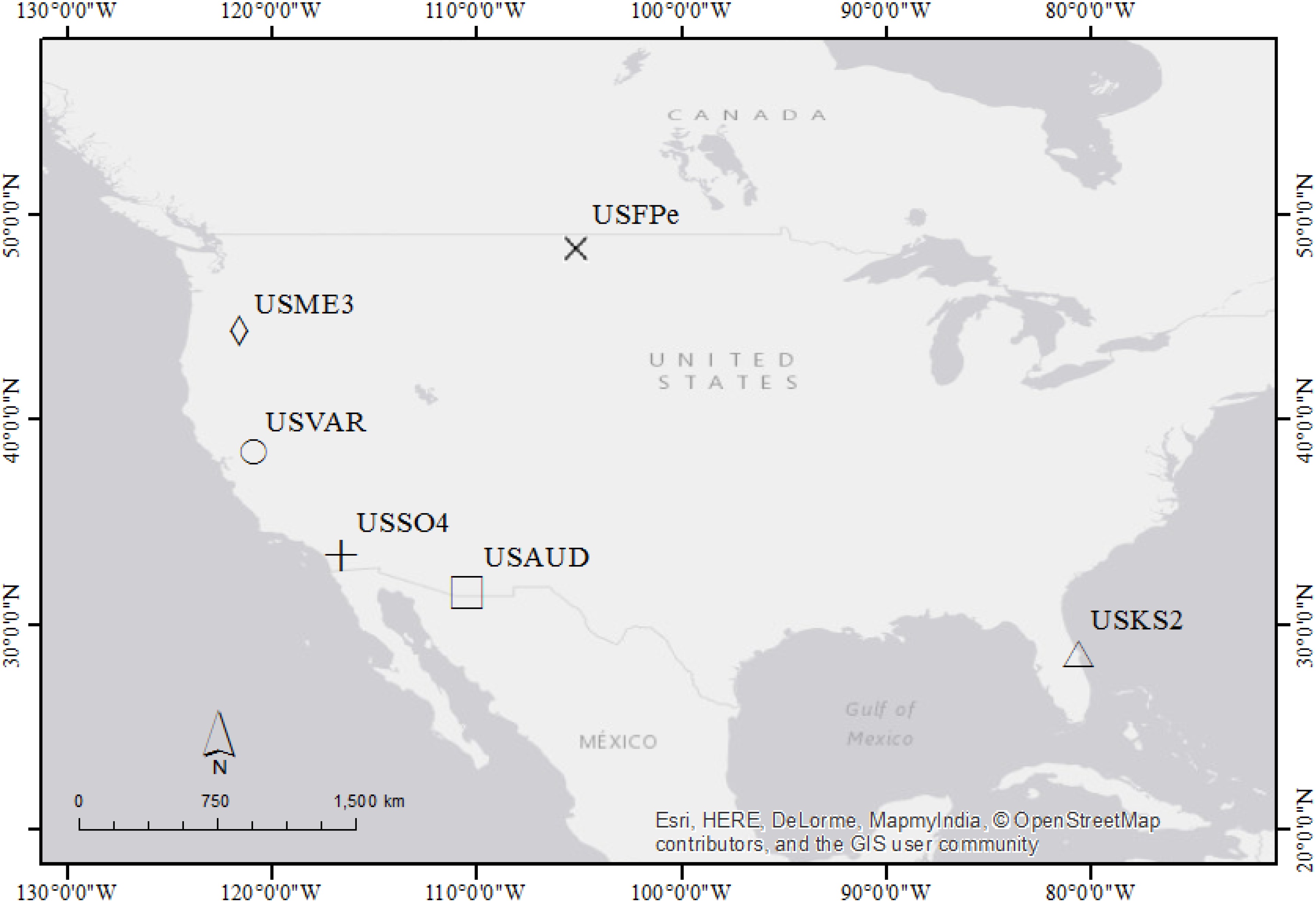
2.1. Study Area

| Site Name | ID | Latitude (º) | Longitude (º) | Elev. (m) | IGBP | CLIM | EC Data | EC Data Used |
|---|---|---|---|---|---|---|---|---|
| Audubon | USAUD | 31.59 | −110.51 | 1469.0 | GRA | Bsh | 2002–2005 | 2003, 2004, 2005 |
| Fort Peck | USFPe | 48.30 | −105.10 | 634.0 | GRA | Bsk | 2000–2006 | 2004, 2005, 2006 |
| Vaira Ranch-Ione | USVAR | 38.41 | −120.95 | 129.0 | GRA | Csa | 2001–2006 | 2004, 2005, 2006 |
| Kennedy Space Center (scrub oak) | USKS2 | 28.60 | −80.67 | 3.0 | CSH | Cfa | 2000–2006 | 2005, 2006 |
| Sky Oaks-new stand | USSO4 | 33.38 | −116.64 | 1429.0 | CSH | Csa | 2004–2006 | 2004, 2005, 2006 |
| Metolius-second young aged pine | USME3 | 44.31 | −121.60 | 1005.0 | ENF | Csb | 2004–2005 | 2004, 2005 |
2.2. Data and Data Processing
2.2.1. EC Flux Tower Data
2.2.2. MODIS-GPP Data (GPPm)
2.3. Analytical Methods
2.3.1. Regression and Agreement Analyses (Annual Basis)
2.3.2. Regression and Agreement Analyses (Temporal Dynamics)
3. Results and Discussion
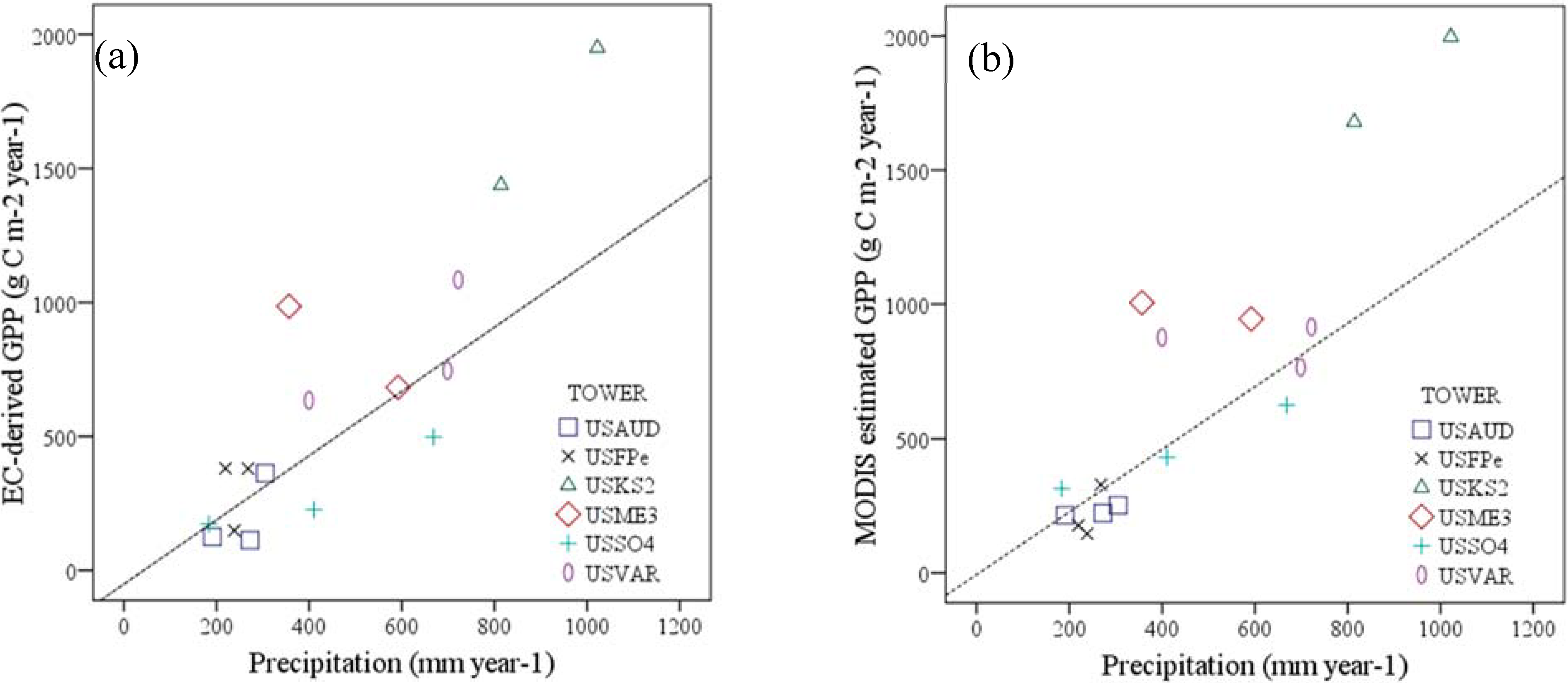
3.1. Suitability of the MODIS GPP Product to Estimate Annual GPP in Shrublands and Grasslands in Water Deficient Areas.
| Tower | Year | GPPec | GPPm | E (%) | Precip |
|---|---|---|---|---|---|
| USAUD | 2003 | 113.1 | 223.5 | 97.6 | 272.0 |
| 2004 | 125.1 | 214.8 | 71.6 | 191.2 | |
| 2005 | 362.9 | 252.1 | −30.5 | 305.6 | |
| USFP | 2004 | 380.2 | 329.4 | −13.4 | 268.0 |
| 2005 | 381.2 | 177.8 | −53.4 | 219.2 | |
| 2006 | 149.1 | 146.2 | −1.9 | 238.4 | |
| USVAR | 2004 | 635.1 | 875.7 | 37.9 | 399.2 |
| 2005 | 1084.8 | 914.5 | −15.7 | 721.6 | |
| 2006 | 745.7 | 766.9 | 2.8 | 698.4 | |
| USKS2 | 2005 | 1950.8 | 1997.1 | 2.4 | 1022.4 |
| 2006 | 1438.4 | 1679.2 | 16.7 | 814.4 | |
| USSO4 | 2004 | 227.2 | 431.7 | 90.0 | 410.4 |
| 2005 | 498.1 | 626.3 | 25.7 | 668.8 | |
| 2006 | 173.5 | 314.4 | 81.2 | 184.0 | |
| USME3 | 2004 | 985.9 | 1005.1 | 1.9 | 365.8 |
| 2005 | 683.6 | 944.5 | 38.2 | 592.0 |
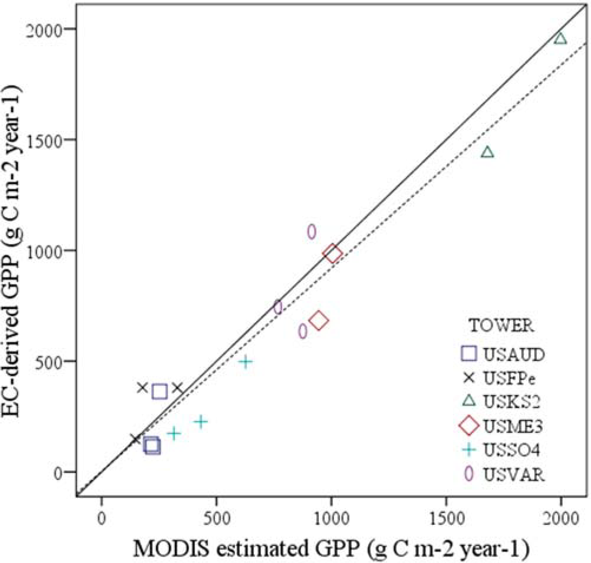
| Variable Y | Variable X | Dataset | r2 | SEE |
|---|---|---|---|---|
| GPPec | GPPm | 1 | 0.77 | 149.26 |
| 2 | 0.94 | 143.36 | ||
| 3 | 0.93 | 142.57 | ||
| GPPec | Precip | 1 | 0.68 | 175.11 |
| 2 | 0.83 | 233.86 | ||
| 3 | 0.75 | 267.41 | ||
| GPPm | Precip | 1 | 0.71 | 159.51 |
| 2 | 0.83 | 249.28 | ||
| 3 | 0.77 | 272.02 |

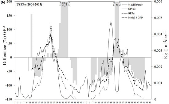
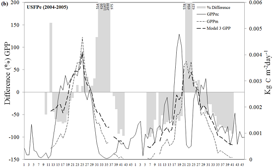
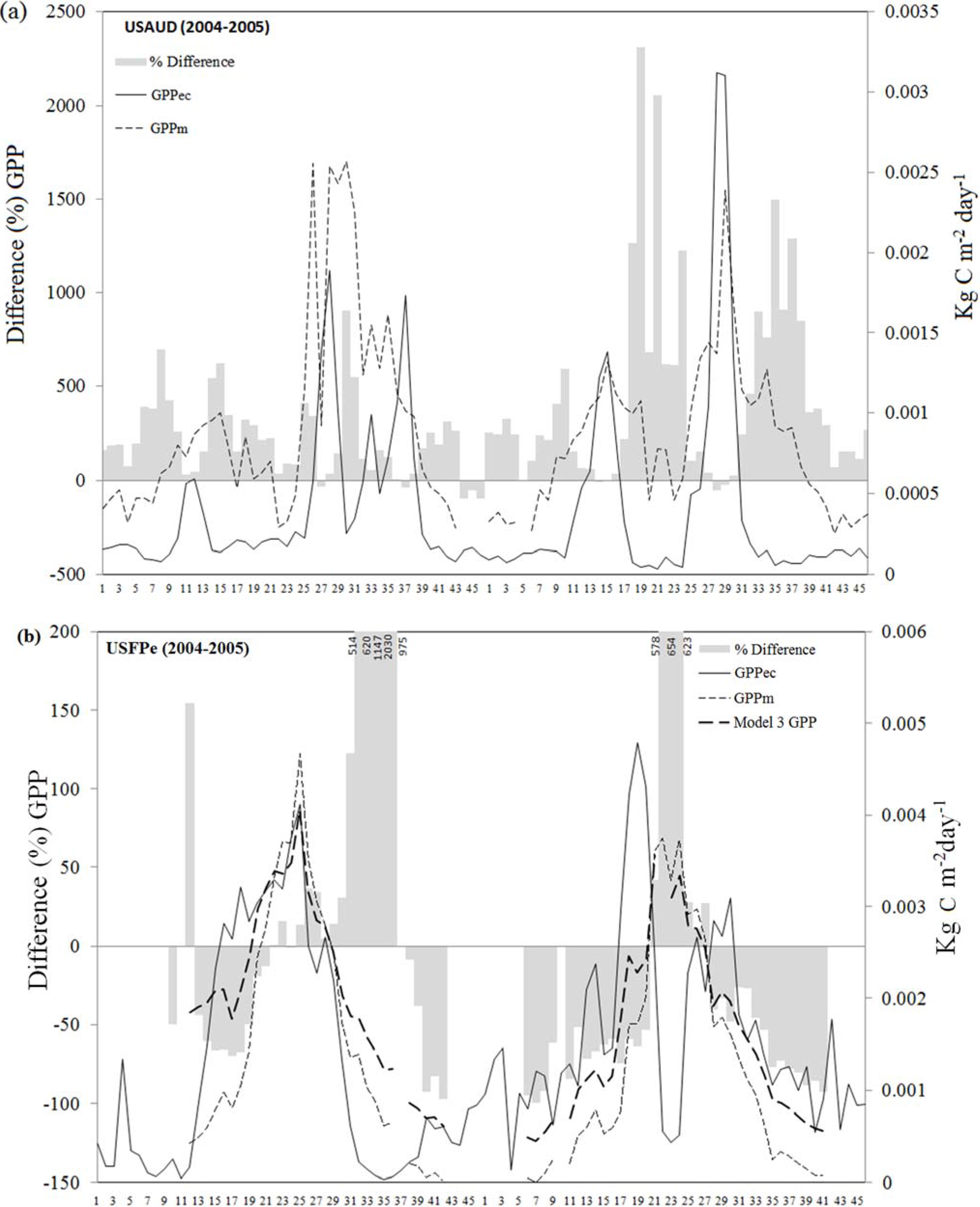
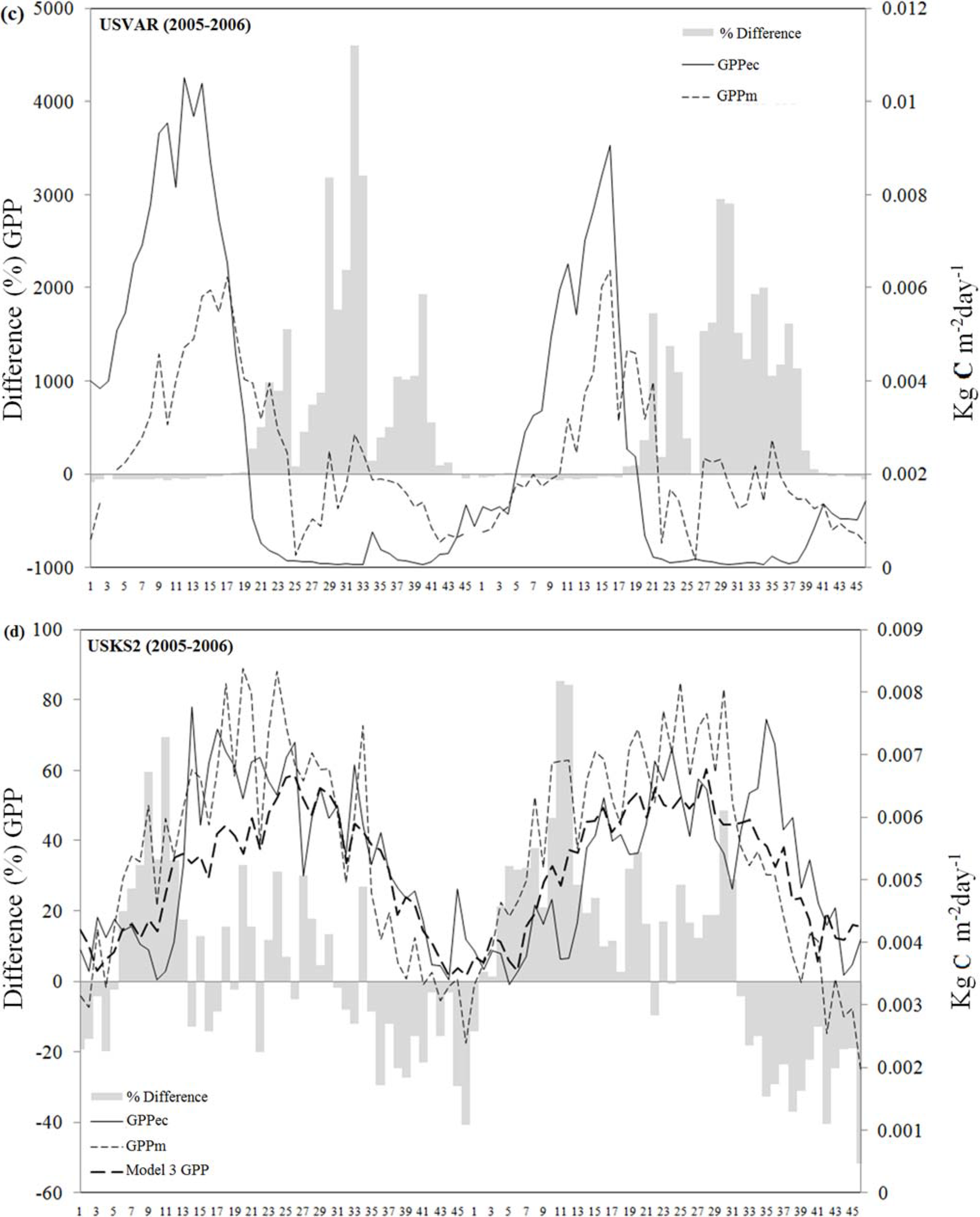
3.2. Suitability of the MODIS GPP Product to Estimate Temporal Dynamics of the Carbon Fluxes at Eight-Day Intervals.


| Tower | Model 1 | Model 2 | Model 3 | |||||
|---|---|---|---|---|---|---|---|---|
| Year | r2/ #ρ2 | SEE | r2/ #ρ2 (n) | SEE | r2/ #ρ2 | SEE | Var | |
| USAUD | 2003 | 0.58 # | - | 0.03 # (96) | - | 0.18 # | Ts | |
| 2004 | 0.29 # | - | ||||||
| 2005 | 0.18 # | - | ||||||
| USFPe | 2004 | 0.32 | 0.73 | 0.44 (62) | 0.89 | 0.52 | 0.83 | GPPm, SWC |
| 2005 | 0.50 | 0.81 | ||||||
| 2006 | 0.57 | 0.49 | ||||||
| USVAR | 2004 | 0.02 # | - | 0.13 # (136) | - | 0.60 # | SWC | |
| 2005 | 0.37 # | - | ||||||
| 2006 | 0.14 # | - | ||||||
| USKS2 | 2005 | 0.54 | 0.89 | 0.49 | 0.88 | 0.65 | 0.75 | Ts, Rg |
| 2006 | 0.51 | 0.81 | (82) | |||||
| USSO4 | 2004 | 0.39 | 0.38 | 0.46 (104) | 0.51 | 0.50 | 0.50 | GPPm, Rg |
| 2005 | 0.46 | 0.57 | ||||||
| 2006 | 0.36 | 0.39 | ||||||
| USME3 | 2004 | 0.78 | 0.85 | 0.69 | 0.92 | 0.75 | 0.83 | GPPm, Ta |
| 2005 | 0.65 | 0.84 | (89) | |||||
3.3. Conditions/Variables Which May Affect the Suitability of the MODIS GPP Product for Estimating C Temporal Dynamics in Shrublands and Grasslands in Water Deficient Areas
4. Conclusions
Acknowledgments
Author Contributions
Conflicts of Interest
References
- Jarvis, P.G. Global change and terrestrial ecosystems in monsoon Asia. Vegetation 1995, 121, 157–174. [Google Scholar] [CrossRef]
- Coops, N.C.; Black, T.A.; Jassal, R.S.; Trofymow, J.A.; Morgenstern, K. Comparison of MODIS, eddy covariance determined and physiologically modelled gross primary production (GPP) in a Douglas-fir forest stand. Remote Sens. Environ. 2007, 107, 385–401. [Google Scholar] [CrossRef]
- Goulden, M.L.; Daube, B.C.; Fan, S.M.; Sutton, D.J.; Bazzaz, A.; Munger, J.W.; Wofsy, S.C. Physiological responses of a black spruce forest to weather. J. Geophys. Res. Atmos. 1997, 102, 28987–28996. [Google Scholar] [CrossRef]
- Huang, H.; Zhang, J.; Meng, P.; Fu, Y.; Zheng, N.; Gao, J. Seasonal variation and meteorological control of CO2 flux in a hilly plantation in the mountain areas of North China. Acta Meteorol. Sinica 2011, 25, 238–248. [Google Scholar] [CrossRef]
- Morgenstern, K.; Black, T.A.; Humphrey, E.R.; Griffis, T.J.; Drewitt, G.B.; Cai, T.; Nesic, Z.; Livingston, N.J. Sensitivity and uncertainty of the carbon balance of a Pacific Northwest Douglas-fir forest during an El Niño/La Niña cycle. Agr. Forest Meteorol. 2004, 123, 201–219. [Google Scholar] [CrossRef]
- Thomas, M.V.; Malhi, Y.; Fenn, K.M.; Fisher, J.B.; Morecroft, M.D.; Lloyd, C.R.; Taylor, M.E.; McNeil, D.D. Carbon dioxide fluxes over an ancient broadleaved deciduous woodland in southern England. Biogeosciences 2011, 8, 1595–1613. [Google Scholar] [CrossRef]
- Valentini, R.; Matteucci, G.; Dolman, A.J.; Schulze, E.D.; Rebmann, C.; Moors, E.J.; Granier, A.; Gross, P.; Jensen, N.O.; Pilegaard, K.; et al. Respiration as the main determinant of carbon balance in European forests. Nature 2000, 404, 861–865. [Google Scholar] [CrossRef] [PubMed]
- Van Dijk, A.I.J.M.; Dolman, A.J. Estimates of CO2 uptake and release among European forests based on eddy covariance data. Glob. Change Biol. 2004, 10, 1445–1459. [Google Scholar] [CrossRef]
- Gilmanov, T.G.; Aires, L.; Belelli, L.; Barcza, Z.; Baron, V.S.; Beringer, J.; Billesbach, D.; Bonal, D.; Bradford, J.; Ceschia, E.; et al. Productivity, respiration, and light-response parameters of world grassland and agroecosystems derived from flux-tower measurements. Rangeland Ecol. Manag. 2010, 63, 16–39. [Google Scholar] [CrossRef]
- Gebremichael, M.; Barros, A.P. Evaluation of MODIS gross primary productivity (GPP) in tropical monsoon regions. Remote Sens. Environ. 2006, 100, 150–166. [Google Scholar] [CrossRef]
- Wu, C.; Chen, J.M. The use of precipitation intensity in estimating gross primary production in four northern grasslands. J. Arid Environ. 2012, 82, 11–18. [Google Scholar] [CrossRef]
- Ham, J.M.; Knapp, A.K. Fluxes of CO2, water vapor, and energy from a prairie ecosystem during the seasonal transition from carbon sink to carbon source. Agr. Forest Meteorol. 1998, 89, 1–14. [Google Scholar] [CrossRef]
- Heinsch, F.A.; Zhao, M.; Running, S.W.; Kimball, J.S.; Nemani, R.R.; Davis, K.J.; Bolstad, P.V.; Cook, B.D.; Desai, A.R.; Ricciuto, D.M.; et al. Evaluation of remote sensing based terrestrial productivity from MODIS using regional tower eddy flux network observations. IEEE Trans. Geosci. Remote Sens. 2006, 44, 1908–1925. [Google Scholar] [CrossRef]
- Goulden, M.L.; Munger, W.; Fan, S.; Daube, B.C.; Wofsy, S.C. Measurements of carbon sequestration by long-term eddy covariance: Methods and a critical evaluation of accuracy. Glob. Change Biol. 1996, 2, 169–182. [Google Scholar] [CrossRef]
- Desai, A.R.; Richardson, A.D.; Moffa, A.M.; Kattge, J.; Hollinger, D.Y.; Barr, A.; Falge, E.; Noormets, A.; Papale, D.; Reichstein, M.; et al. Cross-site evaluation of eddy covariance GPP and RE decomposition techniques. Agr. Forest Meteorol. 2008, 148, 821–838. [Google Scholar] [CrossRef]
- Turner, D.P.; Urbanski, S.; Wofsy, S.C.; Bremer, D.J.; Gower, S.T.; Gregory, M. A cross-biome comparison of light use efficiency for gross primary production. Glob. Change Biol. 2003, 9, 383–395. [Google Scholar] [CrossRef]
- Baldocchi, D.; Falge, E.; Gu, L.; Olson, R.; Hollinger, D.; Running, S.; Anthoni, P.; Bernhofer, C.; Davis, K.; Evans, R.; et al. FLUXNET: A new tool to study the temporal and spatial variability of ecosystem-scale carbon dioxide, water vapor, and energy flux densities. Bull. Am. Meteorol. Soc. 2001, 82, 2415–2434. [Google Scholar] [CrossRef]
- Xiao, J.; Zhuang, Q.; Law, B.E.; Chen, J.; Baldocchi, D.D.; Cook, D.R.; Oren, D.; Richardson, A.D.; Wharton, S.; Ma, S.; et al. A continuous measure of gross primary production for the conterminous United States derived from MODIS and AmeriFlux data. Remote Sens. Environ. 2010, 114, 576–591. [Google Scholar] [CrossRef]
- Coops, N.C.; Waring, R.H. The use of multi-scale remote sensing imagery to derive regional estimates of forest growth capacity using 3-PGS. Remote Sens. Environ. 2001, 75, 324–334. [Google Scholar] [CrossRef]
- Landsberg, J.J.; Waring, R.H. A generalized model of forest productivity using simplified concepts of radiation-use efficiency, carbon balance, and partitioning. Forest Ecol. Manag. 1997, 95, 209–228. [Google Scholar] [CrossRef]
- Li, Z.Q.; Yu, G.R.; Xiao, X.M.; Li, Y.N.; Zha, X.Q.; Ren, C.Y.; Zhang, L.M.; Fu, Y.L. Modelling gross primary production of alpine ecosystems in the Tibetan Plateau using MODIS images and climate data. Remote Sens. Environ. 2007, 107, 510–519. [Google Scholar] [CrossRef]
- Turner, D.P.; Ritts, W.D.; Cohen, W.B.; Gower, S.T.; Running, S.W.; Zhao, M.; Costa, M.H.; Kirschbaum, A.A.; Ham, J.; Saleska, S.; et al. Evaluation of MODIS NPP and GPP products across multiple biomes. Remote Sens. Environ. 2006, 102, 282–292. [Google Scholar] [CrossRef]
- Drolet, G.G.; Middleto, E.M.; Huemmrich, K.F.; Hall, F.G.; Amiro, B.D.; Barr, A.G.; Black, T.A.; McCaughey, J.H.; Margolis, H.A. Regional mapping of gross light-use efficiency using MODIS spectral indices. Remote Sens. Environ. 2008, 112, 3064–3078. [Google Scholar] [CrossRef]
- Veroustraete, F.; Patyn, J.; Myneni, R.B. Estimating net ecosystem exchange of carbon using the normalized difference vegetation index and an ecosystem model. Remote Sens. Environ. 1996, 58, 115–130. [Google Scholar] [CrossRef]
- Xiao, X.; Hollinger, D.; Aber, J.D.; Goltz, M.; Davidson, E.A.; Zhang, Q.Y. Satellite-based modeling of gross primary production in an evergreen needleleaf forest. Remote Sens. Environ. 2004, 89, 519–534. [Google Scholar] [CrossRef]
- Xiao, X.; Zhang, Q.; Braswell, B.; Urbanski, S.; Boles, S.; Wofsy, S.C.; Moore III, B.; Ojima, D. Modeling gross primary production of a deciduous broadleaf forest using satellite images and climate data. Remote Sens. Environ. 2004, 91, 256–270. [Google Scholar] [CrossRef]
- Running, S.W.; Nemani, R.R.; Heinsch, F.A.; Zhao, M.; Reeves, M.; Jolly, M. A continuous satellite-derived measure of global terrestrial primary productivity: Future science and applications. Bioscience 2004, 56, 547–560. [Google Scholar] [CrossRef]
- Data Assimilation Office (DAO); (Goddard Space Flight Center, Greenbelt, MD, USA). Algorithm Theoretical Basis Document (ATBD). Unpublished word. 2002. [Google Scholar]
- Turner, D.P.; Ritts, W.D.; Zhao, M.; Kurc, S.A.; Dunn, A.L.; Wofsy, S.C.; Small, E.E.; Running, S.W. Assessing interannual variation in MODIS-based estimates of gross primary production. IEEE Trans. Geosci. Remote Sens. 2006, 44, 1899–1907. [Google Scholar] [CrossRef]
- Goerner, A.; Reichstein, M.; Rambal, S. Tracking seasonal drought effects on ecosystem light use efficiency with satellite-based PRI in a Mediterranean forest. Remote Sens. Environ. 2009, 113, 1101–1111. [Google Scholar] [CrossRef]
- Chasmer, L.; Barr, A.; Hopkinson, C.; McCaughey, H.; Treitz, P.; Black, A. Scaling and assessment of GPP from MODIS using a combination of airborne LiDAR and eddy covariance measurements over jack pine forests. Remote Sens. Environ. 2009, 113, 82–93. [Google Scholar] [CrossRef]
- Zhang, L.; Wylie, B.; Loveland, T.; Fosnight, E.; Tieszen, L.L.; Ji, L.; Gilmanov, T. Evaluation and comparison of gross primary production estimates for the Northern Great Plains grasslands. Remote Sens. Environ. 2007, 106, 173–189. [Google Scholar] [CrossRef]
- Köppen, W.; Geiger, R. Das geographische system der klimate. In Handbuch der Klimatologie; Verlag Gebrüder Bornträger: Berlin, Germany, 1936. [Google Scholar]
- Ameriflux Website. Available online: http://public.ornl.gov/ameriflux/ (accessed on 28 November 2014).
- Moffat, A.M.; Papale, D.; Reichstein, M.; Hollinger, D.Y.; Richardson, A.D.; Barr, A.G.; Beckstein, C.; Braswell, B.H.; Churkina, G.; Desai, A.R.; et al. Comprehensive comparison of gap filling techniques for eddy covariance net carbon fluxes. Agr. Forest Meteorol. 2007, 147, 209–232. [Google Scholar] [CrossRef]
- Lasslop, G.; Reichstein, M.; Papale, D.; Richardson, A.D.; Arneth, A.; Barr, A.; Stoy, P.; Wohlfahrt, G. Separation of net ecosystem exchange into assimilation and respiration using a light response curve approach: Critical issues and global evaluation. Glob. Change Biol. 2010, 16, 187–208. [Google Scholar] [CrossRef]
- Reichstein, M.; Falge, E.; Baldocchi, D.; Aubinet, M.; Berbigier, P.; Bernhofer, C.; Buchmann, N.; Falk, M.; Gilmanov, T.; Granier, A.; et al. On the separation of net ecosystem exchange into assimilation and ecosystem respiration: Review and improved algorithm. Glob. Change Biol. 2005, 11, 1424–1439. [Google Scholar] [CrossRef]
- Wolf, S.; Eugste, W.; Potvin, C.; Turner, B.; Buchmann, N. Carbon sequestration potential of tropical pasture compared with afforestation in Panama. Glob. Change Biol. 2011, 17, 2763–2780. [Google Scholar] [CrossRef]
- Oak Ridge National Laboratory Distributed Active Archive Center. MODIS Subsetted Land Products, Collection 5. Available online: http://daac.ornl.gov/MODIS/modis.html (accessed on 28 November 2014).
- Running, S.; Zhao, M. Note on Use of MODIS GPP/NPP (MOD17) Data Set. Available online: ftp://daac.ornl.gov/data/modis_ascii_subsets/C5_MOD17A2/mod17_NTSG.pdf (accessed on 28 November 2014).
- Corder, G.W.; Foreman, D.I. Nonparametric Statistics for Non-Statisticians: A Step-by-Step Approach; Wiley: Hoboken, NJ, USA, 2009. [Google Scholar]
- Zhao, L.; Gu, S.; Yu, G.; Zhao, X.; Li, Y.; Xu, S.; Zhou, H. Diurnal, seasonal and annual variation in net ecosystem CO2 exchange of an alpine shrubland on Qinghai-Tibetan plateau. Glob. Change Biol. 2006, 12, 1940–1953. [Google Scholar] [CrossRef]
- Mu, Q.M.; Heinsch, F.A.; Liu, M.; Tian, H.; Running, S.W. Evaluating water stress controls on primary production in biogeological and remote sensing based models. J. Geophys. Res. 2007, 112. [Google Scholar] [CrossRef]
- NOAA. Drought—Annual 2005. Available online: http://www.ncdc.noaa.gov/sotc/drought/2005/13 (accessed on 28 November 2014).
- Serrano-Ortiz, P. Intercambios De CO2 Entre Atmósfera y Ecosistemas Kársticos: Aplicabilidad De Las Técnicas Comúnmente Empleadas; Universidad de Granada: Granada, Spain, 2008. [Google Scholar]
- Slatyer, R.O. Plant-Water Relationships; Academic Press: New York, NY, USA, 1967. [Google Scholar]
- Jaksic, V.; Kiely, G.; Albertson, J.; Oren, R.; Katul, G.; Leahy, P.; Byrne, K.A. Net ecosystem exchange of grassland in contrasting wet and dry years. Agr. Forest Meteorol. 2006, 139, 323–334. [Google Scholar] [CrossRef]
- Perez-Quezada, J.F.; Bown, H.E.; Fuentes, J.P.; Alfaro, F.A.; Franck, N. Effects of afforestation on soil respiration in an arid shrubland in Chile. J. Arid Environ. 2012, 83, 45–53. [Google Scholar] [CrossRef]
© 2015 by the authors; licensee MDPI, Basel, Switzerland. This article is an open access article distributed under the terms and conditions of the Creative Commons Attribution license (http://creativecommons.org/licenses/by/4.0/).
Share and Cite
Álvarez-Taboada, F.; Tammadge, D.; Schlerf, M.; Skidmore, A. Assessing MODIS GPP in Non-Forested Biomes in Water Limited Areas Using EC Tower Data. Remote Sens. 2015, 7, 3274-3292. https://doi.org/10.3390/rs70303274
Álvarez-Taboada F, Tammadge D, Schlerf M, Skidmore A. Assessing MODIS GPP in Non-Forested Biomes in Water Limited Areas Using EC Tower Data. Remote Sensing. 2015; 7(3):3274-3292. https://doi.org/10.3390/rs70303274
Chicago/Turabian StyleÁlvarez-Taboada, Flor, David Tammadge, Martin Schlerf, and Andrew Skidmore. 2015. "Assessing MODIS GPP in Non-Forested Biomes in Water Limited Areas Using EC Tower Data" Remote Sensing 7, no. 3: 3274-3292. https://doi.org/10.3390/rs70303274