Early Water Stress Detection Using Leaf-Level Measurements of Chlorophyll Fluorescence and Temperature Data

Abstract

The purpose of this paper was to investigate the early water stress in maize using leaf-level measurements of chlorophyll fluorescence and temperature. In this study, a series of diurnal measurements, such as leaf chlorophyll fluorescence (Fs), leaf spectrum, temperature and photosynthetically active radiation (PAR), were conducted for maize during gradient watering and filled watering experiments. Fraunhofer Line Discriminator methods (FLD and 3FLD) were used to obtain fluorescence from leaves spectrum. This simulated work using the SCOPE model demonstrated the variations in fluorescence and temperature in stress levels expressed by different stress factors. In the field measurement, the gradient experiment revealed that chlorophyll fluorescence decreased for plants with water stress relative to well-water plants and T_leaf-T_air increased; the filled watering experiment stated that chlorophyll fluorescence of maize under water stress were similar to those of maize under well-watering condition. In addition, the relationships between the Fs, retrieved fluorescence, T_leaf-T_air and water content were analyzed. The Fs determination resulted to the best coefficients of determination for the normalized retrieved fluorescence FLD/PAR (R² = 0.54), T_leaf-T_air (R² = 0.48) and water content (R² = 0.71). The normalized retrieved fluorescence yielded a good coefficient of determination for T_leaf-T_air (R² = 0.48). This study demonstrated that chlorophyll fluorescence could reflect variations in the physiological states of plants during early water stress, and leaf temperature confirmed the chlorophyll fluorescence analysis results and improved the accuracy of the water stress detection.

1. Introduction

Vegetation water stress is a significant issue that currently affects maize growth and production. Maize is currently regarded as the most important food crop in the world. A focus on maize drought is important for plant growth, sustainable human development, the environment and the economies of countries worldwide. Accurately monitoring drought has always been a focus of research and has attracted the attention of many people [1,2]. Numerous studies have shown that vegetation water stress can be measured using optical and thermal infrared remote sensing, as well as passive and active microwave remote sensing techniques [1,2,3,4,5,6,7,8,9,10]. These techniques exploit surface reflection, surface temperature, brightness, temperature and the backscatter coefficient separately to estimate soil moisture near the surface. Though these methods are widely used, they have several limitations. For example, they lack a direct relationship with the plant physiological state and estimate the plant drought based on the surface information. Thermal infrared remote sensing is a wide and effective method for detecting vegetation stress, and using the canopy temperature to track water stress is considered reliable for monitoring plant water status [4]. However, retrieving canopy component temperatures involve thermal infrared remote sensing problems, such as how to remove the effects of soil background [11], and the relationships between leaf temperature and water level are not clear [12].

Chlorophyll fluorescence is directly related to plant photosynthesis and the physiological state of vegetation. Thus, chlorophyll fluorescence has been used as a powerful, non-destructive and reliable tool in plant physiology for understanding the primary events of photosynthesis and the effects of stress on photochemistry [13,14,15,16]. Under natural sun light, the energy absorbed by the leaf is used in three processes, photochemistry, heat dissipation and chlorophyll fluorescence [17,18]. These three processes compete with each other, and variations in one process can affect the other. Many studies have shown that both chlorophyll fluorescence and photochemistry for plants decrease due to deactivation of antennae to prevent damage by harmful radicals that are formed under stress conditions, while heat dissipation increases aiming to dissipate the extra energy and protect the plant from destroy [19,20,21,22,23,24,25,26]. Therefore, many researchers have focused on chlorophyll fluorescence and have exploited it to monitor water stress [12,15,17,22,23,26,27,28].

To actively measure chlorophyll fluorescence, several chlorophyll fluorescence parameters, including the steady-state chlorophyll fluorescence (Ft), Fm/Fo, photochemical quenching coefficient (PQ) and non-photochemical quenching coefficient (NPQ), are measured using a chlorophyll fluorometer (PAM). These parameters and leaf gas-exchange parameters (CO₂ assimilation rate, transpiration rate, leaf temperature and related parameters) are widely used to study the effects of water stress on the in vivo chlorophyll fluorescence in leaves [29,30,31,32].

Active measurements can estimate the fluorescence effectively at the leaf. In addition, the methods based on remote sensing have been developed for detecting vegetable stress: (i) The fluorescence lidar system has been used to obtain plant fluorescence images to determine the vegetation status [33]. (ii) Hyperspectral remote sensing can provided new methods for detecting sun-induced chlorophyll fluorescence and has made remarkable progress in recent years. It is then possible to detect vegetation stress using hyperspectral remote sensing on a large scale. Thermal and hyperspectral images have been obtained from an unmanned aerial vehicle (UAV), and field measurement (including the leaf water potential measurement, stomatal conductance measurement, and leaf chlorophyll fluorescence measurement) was used to assess the vegetation water stress [12,24,25,34]. The chlorophyll index (DCI = D₇₀₅/D₇₂₂) [29], in-filling method [22], fluorescence ratios (F685/F735, F452/F685 and F452/F735) derived from the fluorescence spectrum [30], and reflectance index D715/D705 derived from the first derivative reflectance spectrum [23] were used to detect plant variations associated with some environmental factors that affect plant growth and productivity. The fluorescence, canopy water content and MODIS EVI data were retrieved from the Greenhouse Gases Observing Satellite GOSAT, and were used to analyze the water stress in Amazonia at a global scale [35].

The purpose of this paper is to use chlorophyll fluorescence and leaf temperature data to detect water stress in winter wheat. Chlorophyll fluorescence is obtained from active measurement and passive measurement. The relationship between photosynthesis and chlorophyll fluorescence reveals that chlorophyll fluorescence can be a very powerful tool for studying plant performance, especially when coupled with other noninvasive measurements, such as absorption spectroscopy, gas analyses and infrared thermometry [36]. Therefore, in this paper, the chlorophyll fluorescence and leaf temperature on the leaf scale are combined to detect water stress in potted maize. Using this combination, the accuracy of detecting plant stress may improve.

2. Materials and Methods

2.1. Experimental Setup

The experimental site was located in the biological park in Beijing Normal University, which is in a sunny position with no high objects to block the sunlight. Potted maize was selected as the object of research. The soils in the plots at the study site all had typical silt loam profiles with uniform texture. Maize plants were planted in 20 plastic buckets in June 2013 and fertilized at the V6 stage (vegetative stage, six collars). Three maize plants were grown in each plastic bucket, and after some time, the best plants were kept and the others were removed. At the end, there was one maize plant in one plastic bucket. In addition, all maize was protected from rainfall using an umbrella to guarantee the accuracy of the water stress experiment. The water conditions were controlled during the maize growth process. The normal maize water consumption was 1860–4440 m³/ha over the entire life of the plant [32]. The maize was watered four times during the following stages: before planting, V12 (vegetative stage, 12 collars), V15 (vegetative stage, 15 collars) and R (reproductive stage) [37]. During the V12 stage, lacking water or nutrients will drastically affect yield; thus, it was important to add water at this stage. Generally, 1/4 of the normal watering amount was applied at each of the maize growth stages mentioned above. In this experiment, we assumed that the normal maize water consumption at one stage was 750 m³/ha, and according to the volume of plastic bucket (height 40 cm, diameter 30 cm), 5×10⁻³ m³ water was considered as a normal amount during the V12 stage. All maize was divided into four groups, S1, S2, S3 and S4. The four groups were treated as explained in Table 1.

Table 1. Watering conditions.

Date	Water Condition	Water Consumption (m3/per barrel)
		S1	S2	S3	S4
2 July	The gradient watering	0	1.25×10−3	2.5×10−3	5×10−3
5 July	The filled watering	5×10−3	3.75×10−3	2.5×10−3	0

Table 1. Watering conditions.

Date	Water Condition	Water Consumption (m3/per barrel)
		S1	S2	S3	S4
2 July	The gradient watering	0	1.25×10−3	2.5×10−3	5×10−3
5 July	The filled watering	5×10−3	3.75×10−3	2.5×10−3	0

In this experiment, three measurements were carried out. These measurements were used to analyze the relationships between chlorophyll fluorescence and the plant physiological state. For each measurement, the leaf spectrum, leaf chlorophyll fluorescence, PAR and soil water content were collected. The measurement arrangement is described in Table 2.

Table 2. Measurement timetable.

Date	Stage	Water	Measure Parameters	Time
2July	V12	at night	Leaf spectrum, chlorophyll fluorescence, PAR and soil water content	9:00 am
				11:40 am
				14:30 pm
				16:40 pm
5 July	V12	at night	Leaf spectrum, chlorophyll fluorescence, PAR and soil water content leaf temperature	9:30 am
				11:30 am
				14:30 pm
				16:00 pm
6 July	V12	-	Leaf spectrum, chlorophyll fluorescence, PAR and soil water content leaf temperature	10:00 am

Table 2. Measurement timetable.

Date	Stage	Water	Measure Parameters	Time
2July	V12	at night	Leaf spectrum, chlorophyll fluorescence, PAR and soil water content	9:00 am
				11:40 am
				14:30 pm
				16:40 pm
5 July	V12	at night	Leaf spectrum, chlorophyll fluorescence, PAR and soil water content leaf temperature	9:30 am
				11:30 am
				14:30 pm
				16:00 pm
6 July	V12	-	Leaf spectrum, chlorophyll fluorescence, PAR and soil water content leaf temperature	10:00 am

2.2. Data Collection

Meteorological, leaf spectrum measurements and leaf chlorophyll fluorescence data were collected outdoors under natural solar illumination at several times (Table 2) from the four maize groups. The measurements were collected under clear sky conditions, and using fully expanded maize ear leaves that represented the current growth conditions of the maize.

Field data, including PAM, spectrum and soil water content data, were measured for three days. During the measuring phase, maize was in the V12 stage. Here, the fluorescence that was measured by PAM was marked as Fs, and the fluorescence that was computed from the leaf spectrum using the FLD or 3FLD method was marked as FLD or 3FLD, respectively. The normalized fluorescence was computed by FLD or 3FLD and divided by PAR (marked as FLD/PAR or 3FLD/PAR). In this experiment, the maize was divided into four groups, with four barrel maize plants in each group. In the following analysis, the mean value of each group was used.

2.2.1. PAR Data and Soil Water Content Data Collection

In this study, PAR was measured using a QSO-S PAR Photon Flux sensor (Decagon Devices, USA). The soil moisture was measured using an EC-5 volumetric water content sensor. The data were registered by an EM50 digital/analog data logger. Two points should be noted. (i) First, the PAR measurement was synchronous with the leaf spectral measurements. (ii) Second, the EC-5 volumetric water content sensor was set at a depth of 5 cm below the soil surface.

2.2.2. Leaf Spectral Data Collection

Leaf spectral data were acquired using a high-resolution spectrometer (HR4000) (Ocean Optics, USA), which has been widely used to measure plant spectral information and extract fluorescence data [25,34,38,39]. The HR4000 spectrometer shows a spectral range of 720–800 nm and a spectral resolution of 0.05 nm. Absolute radiance calibration was performed by the Institute of Atmospheric Physics at the Chinese Academy of Sciences. To protect the HR4000 machine from the effects of air temperature, the HR4000 machine was housed in a thermally insulated box to maintain a stable internal temperature and reduce dark current drift [38]. The middle of one leaf from one bucket was measured three times, and the mean value was used for analysis. Radiance-based methods, including FLD and 3FLD, were used to retrieve the fluorescence.

2.2.3. Leaf Fluorescence Measurements

The leaf fluorescence was measured using high-performance field and laboratory chlorophyll Fluorescence PAM-2500 (Heinz Walz GmbH, Germany), which is widely applied in photosynthesis research and in plant eco- and stress-physiology [40]. The Fo and Fm were recorded in the dark-acclimated state. In this case, Fo is the basic chlorophyll fluorescence yield recorded under low measuring light intensities and Fm is the maximum chlorophyll fluorescence yield when the photosystem II reaction centers are closed by a Saturation Pulse. The three following parameters were recorded in the light-exposed state: (i) Fo is the minimum chlorophyll fluorescence yield in the state of open photosystem II reaction centers; (ii) Fm is the maximum chlorophyll fluorescence yield when the photosystem II reaction centers are closed due to a strong light pulse; and (iii) Ft represents the fluorescence during steady-state photochemical levels, which are also marked as Fs. Here, the Fs parameter was used to indicate the current fluorescence. The leaf that was measured by PAM was consistent with that measured by HR4000.

2.2.4. Leaf Temperature Measurement

The leaf temperatures were measured using the infrared thermometer, Testo 845. The emissivity was set to 0.99, and the accuracy was ±0.75 °C between −35 and +75 °C. To ensure the accuracy and comparability of the experiment result, leaf temperature measurements were collected at a time that was consistent with the other measurements. Air temperature was obtained from the automatic weather station in the Beijing Olympic park which is close to the experimental site (Beijing Normal University). Leaf temperature is affected by air temperature; therefore, air temperature was used to correct leaf temperature, marked as T_leaf-T_air.

2.3. FLD and 3FLD Methods

The FLD method, which was developed by Plascyk (1975) and Plascyk and Cabriel (1975) [41,42], forms the basis of all radiation-based methods. The FLD requires two flux measurements, one inside the Fraunhofer line and one outside the Fraunhofer line [43]. Because of the fluorescence, an in-filling effect occurs on the real fluxes in the oxygen absorption bands (O₂-A and O₂-B). For application, FLD is computed using the mathematical operation of the solar irradiance and target radiance inside and outside the Fraunhofer line:

$$\text{FLD}=\frac{\mathrm{E}\left({\mathrm{\lambda }}_{\text{out}}\right)\cdot \mathrm{L}\left({\mathrm{\lambda }}_{\text{in}}\right)-\mathrm{L}({\mathrm{\lambda }}_{\text{out}})\cdot \mathrm{E}\left({\mathrm{\lambda }}_{\text{in}}\right)}{\mathrm{E}\left({\mathrm{\lambda }}_{\text{out}}\right)-\mathrm{E}\left({\mathrm{\lambda }}_{\text{in}}\right)}$$

(1)

where E(λ_out) is the solar irradiance outside the Fraunhofer line, E(λ_in) is the solar irradiance inside the Fraunhofer line, L(λ_out) is the target radiance outside the Fraunhofer line, and L(λ_in) is the target radiance inside the Fraunhofer line. In this paper, λ_out was 766.84 nm and λ_in was 760.45 nm.

For the 3FLD method, two bands replaced the band outside the Fraunhofer line, one on the left shoulder of the Fraunhofer well and one on the right. Compared with the FLD method, the 3FLD method resulted in a more accurate fluorescence calculation.

$$3\text{FLD}=\frac{\mathrm{L}\left({\mathrm{\lambda }}_{\text{in}}\right)-\frac{\mathrm{E}\left({\mathrm{\lambda }}_{\text{in}}\right)\times ({\mathrm{w}}_{\text{left}}\times \mathrm{L}\left({\mathrm{\lambda }}_{\text{left}}\right)+{\mathrm{w}}_{\text{right}}\times \mathrm{L}\left({\mathrm{\lambda }}_{\text{right}}\right))}{{\mathrm{w}}_{\text{left}}\times \mathrm{E}\left({\mathrm{\lambda }}_{\text{left}}\right)+{\mathrm{w}}_{\text{right}}\times \mathrm{E}\left({\mathrm{\lambda }}_{\text{right}}\right)}}{1-\frac{\mathrm{E}\left({\mathrm{\lambda }}_{\text{in}}\right)}{{\mathrm{w}}_{\text{left}}\times \mathrm{E}\left({\mathrm{\lambda }}_{\text{left}}\right)+{\mathrm{w}}_{\text{right}}\times \mathrm{E}\left({\mathrm{\lambda }}_{\text{right}}\right)}}$$

(2)

$${\mathrm{w}}_{\text{left}}=\frac{{\mathrm{\lambda }}_{\text{in}}-{\mathrm{\lambda }}_{\text{left}}}{{\mathrm{\lambda }}_{\text{right}}-{\mathrm{\lambda }}_{\text{left}}}, {\mathrm{w}}_{\text{right}}=\frac{{\mathrm{\lambda }}_{\text{right}}-{\mathrm{\lambda }}_{\text{left}}}{{\mathrm{\lambda }}_{\text{right}}-{\mathrm{\lambda }}_{\text{left}}}$$

where L(λ_left) and L(λ_right) represent the target radiances in the left and right shoulders of the Fraunhofer well, respectively. In addition, E(λ_left) and E(λ_right) represent the solar irradiance in the left and right shoulder of the Fraunhofer well, respectively, and w_left and w_right are the weights of two bands outside the Fraunhofer line. In this paper, λ_right was 766.84 nm, λ_in was 760.45 nm and λ_left was 759.22 nm.

2.4. SCOPE Model

The SCOPE (Soil Canopy Observation, Photochemistry and Energy fluxes) model is a vertical (1-D) integrated radiative transfer and energy balance model [19,44,45,46]. It contains the radiation transfer and energy balance module and can simulate spectra from 0.4 to 50 µm, including the visible, near and short-wave infrared and the thermal domains, with resolutions of 1, 1, 100 and 1000 nm, respectively [47]. The SCOPE model can simulate the fluorescence in the canopy by using the radiation transfer module and leaf biochemical model.

In this study, SCOPE was used to illustrate the variation tendencies of fluorescence and canopy temperature under stress conditions. The input parameters of SCOPE were as also set as default parameters, and the time step was 30 min. In addition, the meteorological data in Baoding, Hebei province, China, was used as input to derive the SCOPE model, and the results showed that the variations of some input parameters did not result in significant variations in fluorescence or temperature trends; therefore, these results are not presented here.

The SCOPE model is not only used in healthy plants but is also suitable for vegetation under stress conditions. In SCOPE, the parameter stress factor can be used to set a value that shows the stress factor to reduce the maximum carboxylation capacity (V_cmax) in a biochemical module, such as soil moisture, leaf age, etc. In addition, V_cmax is an important control parameter of the photosynthesis capacity and varies substantially in space and time in response to environmental control [47]. By varying the stress factor in the SCOPE model, different water stress effects on the fluorescence and canopy temperature can be observed. When the stress factor was set to 1.0, the plant was not under stress.

In the SCOPE model, the following input parameters are:

(i)

PROSPECT parameters, such as the chlorophyll a + b content, dry matter content, leaf water equivalent layer, senescent material fraction, leaf thickness parameters and thermal reflectance and transmittance;

(ii)

Leaf Biochemical parameters, including the maximum carboxylation capacity, stomatal conductance parameter, photochemical pathway, extinction coefficient, respiration and temperature response;

(iii)

Fluorescence quantum yield efficiency at the photosystem level;

(iv)

Soil parameters, including soil spectrum, soil resistance, soil reflectance in the thermal range, heat capacity of the soil, specific mass of the soil and soil moisture content;

(v)

Canopy geometry parameters, including leaf area index, vegetation height, canopy structure and leaf width;

(vi)

Meteorological data, including measurement height, incoming shortwave and longwave radiation, air temperature, air pressure, atmospheric vapor pressure, wind speed, and atmospheric CO₂ and O₂ concentrations;

(vii)

Aerodynamic data, including roughness length for the momentum of the canopy, height, leaf drag coefficient, and resistance;

(viii)

Time series information (only for daily simulation); and

(ix)

Three observation angles (solar zenith angle, observation zenith angle, and the azimuthal difference between solar and observation angles).

3. Results and Discussion

3.1. The Results of the SCOPE Simulation

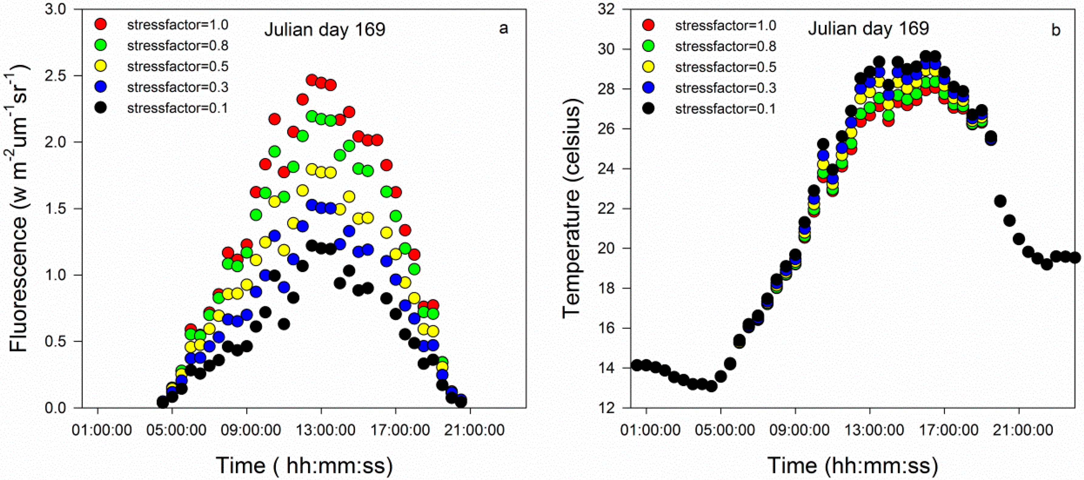
3.1.1. Variations in Chlorophyll Fluorescence and Canopy Temperature under Stress Conditions

Fluorescence from the morning to afternoon gradually increased to a maximum value before decreasing to nearly zero. The fluorescence peaked at approximately midday (Figure 1a). During the early morning or late night hours, no fluorescence occurred over a short period because the leaves did not absorb sunlight during those periods. When plants are in a healthy environment (stressfactor = 1.0), the fluorescence is much higher than when plants are stressed. As a drought becomes more intense, the fluorescence decreases quickly. Compared with fluorescence under different stress conditions, the extents of changes in fluorescence were relatively large around midday and small during the early morning and late afternoon.

The canopy temperature first decreased to its lowest point during the early morning and gradually increased to reach its peak before decreasing again (Figure 1b). A small trough was observed at 13 pm, potentially due to stomatal closure to protect the plant from damage, known as the midday depression of photosynthesis. When vegetation is under stress, the canopy temperature of maize is larger than when the plants are in well-watered conditions.

Figure 1. (a) Time series of the fluorescence. (b) Time series of the canopy temperature.

Figure 1. (a) Time series of the fluorescence. (b) Time series of the canopy temperature.

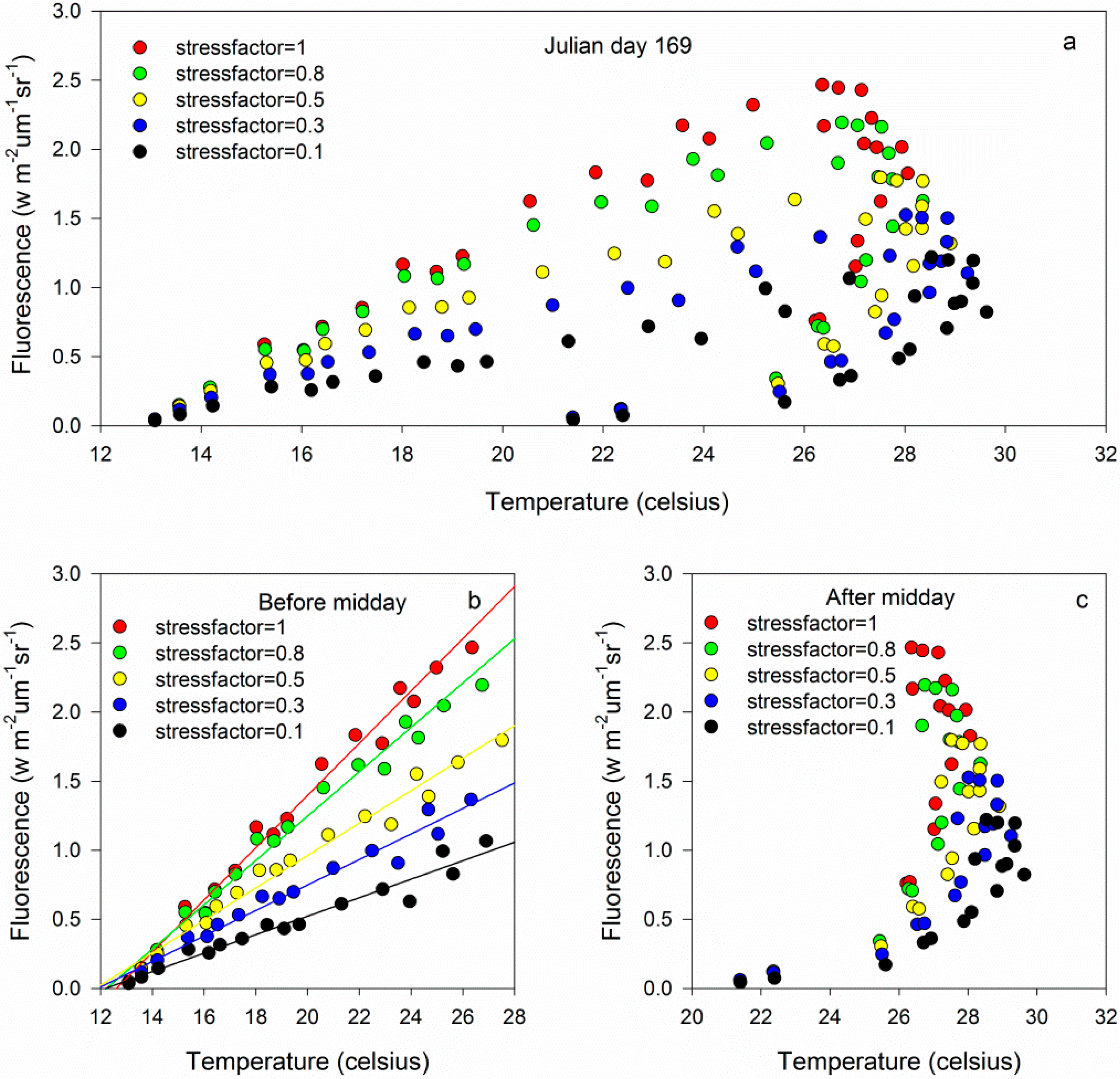
3.1.2. Relationships between Chlorophyll Fluorescence and Canopy Temperatures on the Canopy

Chlorophyll fluorescence and canopy temperature were positively related before becoming negatively related (Figure 2a). A turning point occurred during the daily cycle. Before mid-day, a good linear relationship was observed between the fluorescence and canopy temperature. The slope of this linear relationship varied with the water status (Figure 2b). In this period, chlorophyll fluorescence and temperature gradually increased. The rate of the chlorophyll fluorescence increase declined slowly as stress became more severe, and the rate of temperature remained stable. After midday, the relationship between the fluorescence and canopy temperature was nonlinear, complicated (Figure 2c) and varied with the stress level. When the plant was a healthy maize plant, the maximum temperature was 27 °C, and temperature varied gradually. In addition, the chlorophyll fluorescence declined remarkably in this case. As the stress became more severe (stress factor ranged from 1.0 to 0.1), the maximum temperature slightly increased, and the range of temperature variation gradually increased. Simultaneously, the range of chlorophyll fluorescence decreased. This decrease revealed that heat dissipation played an important role in energy consumption in the afternoon. In addition, using the temperature and chlorophyll fluorescence together can more accurately assess water stress.

Figure 2. Relationships between the fluorescence and canopy temperature: (a) Full day, (b) before midday and (c) after midday.

Figure 2. Relationships between the fluorescence and canopy temperature: (a) Full day, (b) before midday and (c) after midday.

3.2. Analysis of the Field Data

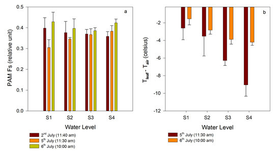
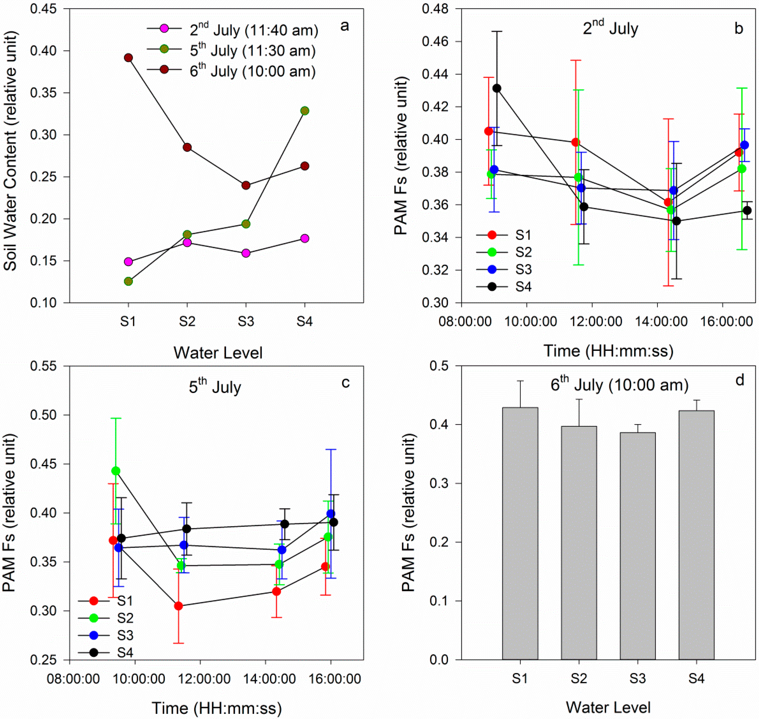
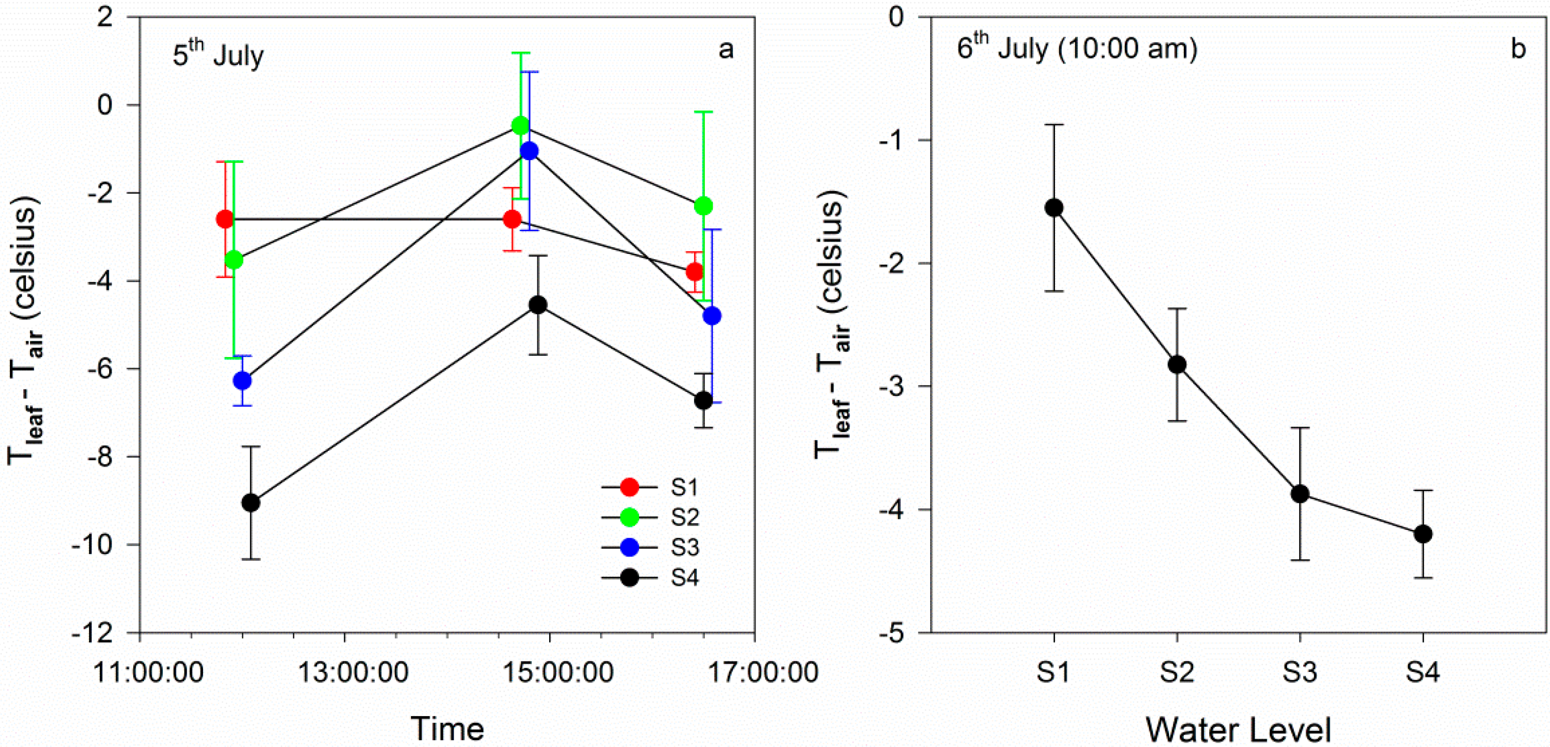
3.2.1. Time Series of Chlorophyll Fluorescence and Leaf Temperature at Different Water Levels

To analyze variations in chlorophyll fluorescence and leaf temperature under water stress conditions, three days of field data were compared.

On 2 July, similar soil water contents for the four groups were measured (Figure 3a). However, the Fs values for the four groups were different during the morning and similar in the afternoon (Figure 3b). When the measurement was finished, gradient watering was applied. The S1 group was treated with no water, the S2 group was treated with ¼ of the normal water volume, the S3 group was treated with ½ of the normal water volume, and the S4 group was treated with the normal water volume.

On 5 July, the Fs in S1 was low and the Fs in the S4 group varied from small to large relative to the values observed on 2 July. Because S3 was treated with more water than S2, the Fs in the S3 group was larger than that in S2 (Figure 3c). The results of the gradient watering indicated that well-watered maize plants had a greater fluorescence than those under water stress. The results of the simulation using the SCOPE model indicated that the fluorescence increased before decreasing, and Zarco-Tejada et al. demonstrated that these results, obtained at the field canopy level from an airborne CASI hyperspectral sensor, were consistent with leaf, laboratory, and theoretical levels [48]. Therefore, a comparison can be performed between field data and the SCOPE results. Under water stress conditions, chlorophyll fluorescence decreased and the leaf temperature increased. This result can be observed in the analysis of field data and the simulation analysis of SCOPE. However, this daily trend of chlorophyll fluorescence was not found in the analysis results of Fs, possibly due to the limited number of measurements. The gradient watering experiment indicated that the Fs value was low under water stress but high in well-watered conditions.

Figure 3. (a) Comparison of the soil water content; (b) Daily variations in the PAM Fs on 2 July; (c) Daily variations of PAM Fs on 5 July; (d) PAM Fs for the four groups on 6 July.

Figure 3. (a) Comparison of the soil water content; (b) Daily variations in the PAM Fs on 2 July; (c) Daily variations of PAM Fs on 5 July; (d) PAM Fs for the four groups on 6 July.

After measuring during the day on 5 July, the filled water was applied at night. According to the normal water volume of maize and the first water volume, the second watering was performed (Table 1). After the filled watering, four groups were treated with the same water volume, and the Fs values in these four groups were similar (Figure 3d). For the S1 group, filled water relieved the water stress condition, and the maize recovered from water stress and reached a relatively healthy state. The Fs in the S1 group recovered to the same level as that in the S4 group when filled watering occurred. In addition, the Fs recovered in the S2 and S3 groups, but several differences were observe relative to the S1 group, potentially due to the low soil water content, which resulted in the need for water in the S1 group. The filled watering experiment demonstrated that it was possible to exploit the Fs to detect when the plant is under early water stress. The Fs can detect subtle variations in a plant’s physiological state.

An infrared thermometer was used to measure the leaf temperature, and air temperature was used to correct leaf temperature. T_leaf-T_air on 5 July and on 6 July was analyzed. On 5 July, the four groups were treated with gradient watering. As shown in Figure 4, T_leaf-T_air under the normal watering conditions was lower than that under water stress. At 12:00 am on 5 July, T_leaf-T_air for S1 was obviously higher than that of the other groups, while at 14:30 pm and 16:30 pm, T_leaf-T_air for S2 was higher than that in S1. This result indicated that the relationships between the temperature and water stress level were complicated [34] and that the temperature cannot accurately reflect variations in the physiological state. Figure 4b shows that after filled watering there were some differences for T_leaf-T_air between the four groups. It may be a result of inadequate water absorption.

Figure 4. (a) Daily variations in T_leaf-T_air on 5 July. (b) Variations in T_leaf-T_air at 10:00 am on 6 July.

Figure 4. (a) Daily variations in T_leaf-T_air on 5 July. (b) Variations in T_leaf-T_air at 10:00 am on 6 July.

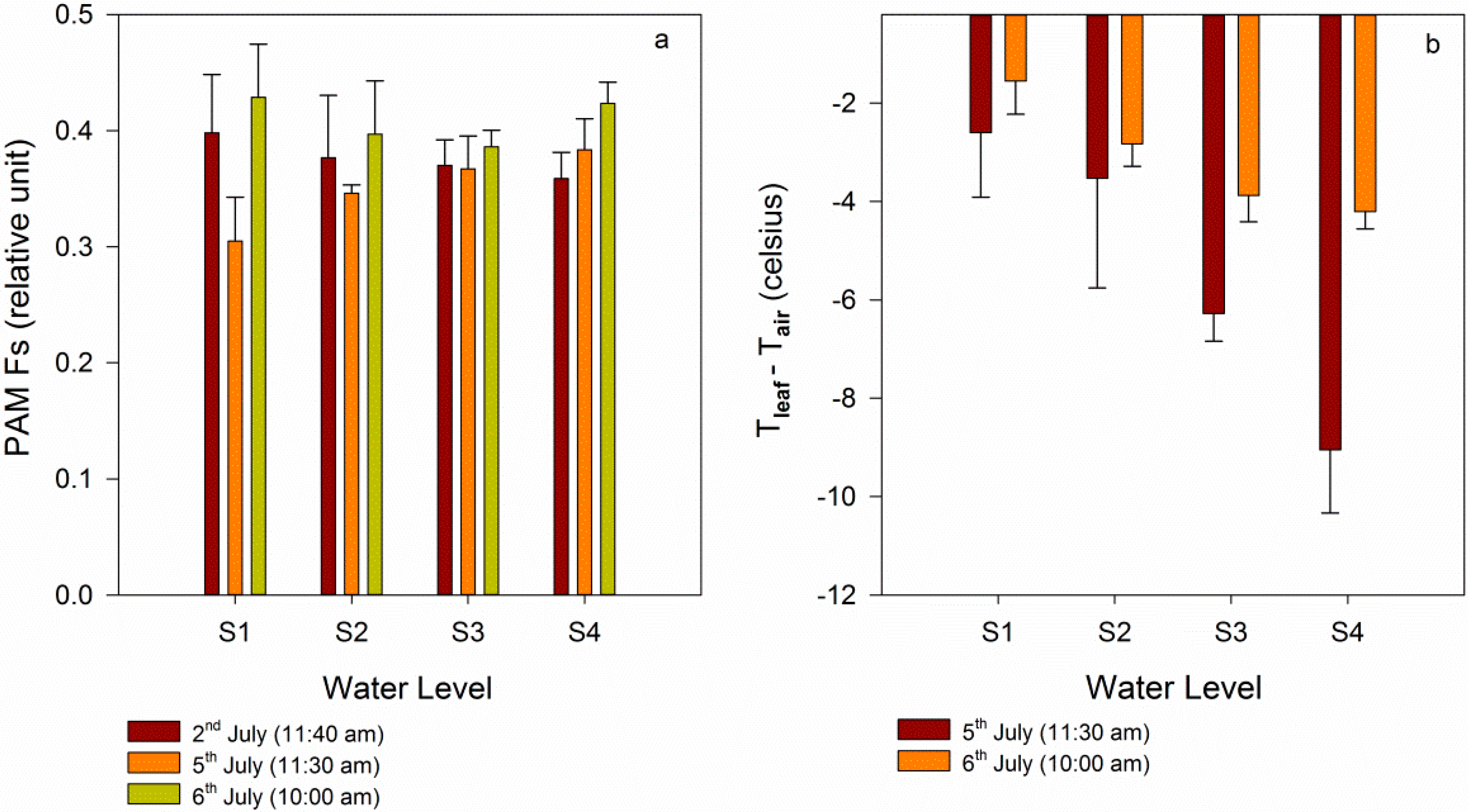
3.2.2. Comparison between Gradient Watering and Filled Watering

To explain the variations in fluorescence and temperature after gradient watering or filled watering, the soil water content, Fs, and temperature data at a certain time within three days were compared. From Figure 3a, the soil water contents in the four groups changed during the two watering times. After the gradient watering, the soil water content in S4 increased quickly, and the soil water content in S2 or S3 increased slightly. In addition, some variations were found in the fluorescence (Figure 5a). On 5 July, the Fs in the S4 group—treated with a normal water volume—was greater than that in the S1 group. According to the water volume, the Fs values in the four groups were arranged in gradient order. When comparing the Fs on 2 July with that on 5 July, the Fs in S4 obviously increased, while that in S1, S2 and S3 decreased. This finding indicated that S1, S2 and S3 were under different degrees of water stress. During the measuring phase, maize was in the V12 stage. At this stage, maize requires water to maintain normal growth. During the addition of filled water, the maize plants in the four groups were given the same volume of water. When comparing the Fs values on 6 July and 5 July, the Fs values of the four groups increased, despite S4 not being given water. The maize in the S4 group remained in a healthy state during the first watering. The same amount of water was given to these four groups, but differences were observed between the Fs values among these four groups, demonstrating differences in the maize physiological state.

Variations in temperature at different water levels can be observed in Figure 5b. When the four groups were given different water volumes, T_leaf-T_air in the lowest water content group was the highest. After filled watering, T_leaf-T_air still increased due to inadequate water absorption. Compared T_leaf-T_air on 5 July with that on 6 July, it was found that the relationship between the temperature and water level was complicated, and the temperature was not sensitive to the variation of soil water content.

Figure 5. Comparison of the Fs (a) and T_leaf-T_air (b) of the four groups.

Figure 5. Comparison of the Fs (a) and T_leaf-T_air (b) of the four groups.

3.2.3. Fluorescence Computed Using Passive Measurements

Radiation-based methods (FLD and 3FLD) were used to extract fluorescence from the leaf spectrum measured by HR4000. Illumination conditions are important for fluorescence. The normalization was calculated by dividing the PAR by the extracted fluorescence from the spectrum (marked as FLD/PAR, 3FLD/PAR) [38].

On 2 July, in Figure 6, the daily variation trend of Fs was the same as that shown in the SCOPE model (Figure 6a and 6d). The Fs increased before gradually decreasing. The Fs in the four groups changed over a small range. After gradient watering, the FLD/PAR in the S4 group was larger than that in the other groups (Figure 6b). The FLD/PAR in S1 was the lowest because S1 group was not given any water. However, the FLD/PAR in S3 was sometimes larger than that in S4. These observations potentially resulted from measured errors in the spectrum and PAR measurements. After the filled watering, the FLD/PAR values in the four groups were similar to each other, and the FLD/PAR in S1 recovered to that of S4 (Figure 6c). In addition, the 3FLD/PAR in the four groups showed the same results (Figure 6d–f). An analysis of the FLD/PAR and 3FLD/PAR in the four groups indicated that chlorophyll fluorescence was closely related with the plant’s physiological state, and could reflect early water stress.

Figure 6. Daily variation in the fluorescence as retrieved by passive measurements: (a), (b) and (c): variations in the fluorescence using FLD on 2, 5 and 6 July; (d), (e) and (f): variations in the fluorescence using 3FLD on 2, 5 and 6 July.

Figure 6. Daily variation in the fluorescence as retrieved by passive measurements: (a), (b) and (c): variations in the fluorescence using FLD on 2, 5 and 6 July; (d), (e) and (f): variations in the fluorescence using 3FLD on 2, 5 and 6 July.

3.2.4. Comparison of the Active and Passive Measurements

The data obtained at 12:00 on 5 July, including the Fs, T, fluorescence retrieved by FLD and 3FLD, and water content, were used to analyze the relationship between the active and passive measurements. The four groups were combined to analyze the relationships between the parameters. The relationships between the fluorescence and other parameters were analyzed, with R² = 0.54 for Fs vs. FLD/PAR (Figure 7a); R² = 0.48 for Fs vs. T_leaf-T_air (Figure 7b); R² = 0.48 for FLD/PAR vs. T_leaf-T_air (Figure 7c); and R² = 0.71 for Fs vs. soil water content (Figure 7d). The performances of FLD/PAR and 3FLD/PAR were similar; therefore, only the comparisons of FLD/PAR with the other parameters are given. A comparison of the active and passive measurements demonstrated the consistency of active and passive measurements, and the close relationships between the fluorescence and soil water contents demonstrated that fluorescence could be used to detect early water stress.

Figure 7. Comparison of the active and passive measurements (a) PAM Fs vs. FLD/PAR; (b) PAM Fs vs. T_leaf-T_air; (c) PAM Fs vs. Soil water content; and (d) FLD/PAR vs. T_leaf-T_air.

Figure 7. Comparison of the active and passive measurements (a) PAM Fs vs. FLD/PAR; (b) PAM Fs vs. T_leaf-T_air; (c) PAM Fs vs. Soil water content; and (d) FLD/PAR vs. T_leaf-T_air.

4. Conclusions

In this study, the SCOPE model was used to simulate chlorophyll fluorescence and temperature in the canopy. Compared with plants in healthy environments, the chlorophyll fluorescence decreased when the plants were stressed and the temperature increased. The relationship between chlorophyll fluorescence and temperature indicated that combining both parameters could improve the accuracy of stress detection. Then, two experiments were designed to illustrate the variations of chlorophyll fluorescence and temperature at different water levels.

A controlled watering experiment was performed to demonstrate that the chlorophyll fluorescence and temperature were closely related with the maize physiological state. Maize in the V12 stage was chosen to research objectives, and two watering were performed to control the water content. By controlling the soil moisture content, variations in the fluorescence and leaf temperature were observed.

The gradient watering experiment showed that the fluorescence for maize was low under water stress. As the water stress became more severe, the temperature gradually increased. Although the fluorescence was closely related with the water level, the relationship between temperature and water level was not clear. This finding suggested that chlorophyll fluorescence could be the best tool for monitoring plant drought. In addition, the temperature results could confirm the results that were obtained using chlorophyll fluorescence.

The filled watering experiment illustrated that chlorophyll fluorescence could be used to monitor early water stress in plants. Filled watering helped relieve water stress in maize without causing physiological tissue damage, resulting in its recovery to a relatively healthy state. In addition, chlorophyll fluorescence of plants under water stressed conditions could increase to levels that are similar to those of plants under well-watered conditions, but the temperature increased due to inadequate water absorption. It also illustrated that chlorophyll fluorescence was more sensitive to variation of soil water content than the temperature.

Based on these experiments, it can be concluded that fluorescence is a useful tool for monitoring early vegetation water stress, and temperature data can be used to confirm the results. In addition, using chlorophyll fluorescence and temperature can compensate for the shortcomings of temperature detection and provide accurate water stress detection.

References

1. Wang, L.; Qu, J.J. Satellite remote sensing applications for surface soil moisture monitoring: A review. Front. Earth Sci. China 2009, 3, 237–247. [Google Scholar] [CrossRef]
2. Peters, A.J.; Walter-Shea, E.A.; Ji, L.; Vina, A.; Hayes, M.; Svoboda, M.D. Drought monitoring with NDVI-based standardized vegetation index. Photogramm. Eng. Remote Sens. 2002, 68, 71–75. [Google Scholar]
3. Fuchs, M.; Tanner, C. Infrared thermometry of vegetation. Agron. J. 1966, 58, 597–601. [Google Scholar] [CrossRef]
4. Jackson, R.D.; Idso, S.; Reginato, R.; Pinter, P. Canopy temperature as a crop water stress indicator. Water Resour. Res. 1981, 17, 1133–1138. [Google Scholar] [CrossRef]
5. Paloscia, S.; Pampaloni, P. Microwave remote sensing of plant water stress. Remote Sens. Environ. 1984, 16, 249–255. [Google Scholar] [CrossRef]
6. Hunt Jr, E.R.; Rock, B.N. Detection of changes in leaf water content using Near- and Middle-Infrared reflectances. Remote Sens. Environ. 1989, 30, 43–54. [Google Scholar] [CrossRef]
7. Gao, B.-C. NDWI—A normalized difference water index for remote sensing of vegetation liquid water from space. Remote Sens. Environ. 1996, 58, 257–266. [Google Scholar] [CrossRef]
8. Walker, J.P. Estimating Soil Moisture Profile Dynamics from Near-Surface Soil Moisture Measurements and Standard Meteorological Data. Ph.D. Thesis, the University of Newcastle, New South Wales, Austrilia, 1999. [Google Scholar]
9. Sandholt, I.; Rasmussen, K.; Andersen, J. A simple interpretation of the surface temperature/vegetation index space for assessment of surface moisture status. Remote Sens. Environ. 2002, 79, 213–224. [Google Scholar] [CrossRef]
10. Vereecken, H.; Weihermüller, L.; Jonard, F.; Montzka, C. Characterization of crop canopies and water stress related phenomena using microwave remote sensing methods: A review. Vadose Zone J. 2012, 11. [Google Scholar] [CrossRef]
11. Bellvert, J.; Marsal, J.; Girona, J.; Zarco-Tejada, P.J. Seasonal evolution of crop water stress index in grapevine varieties determined with high-resolution remote sensing thermal imagery. Irrigation Sci. 2014, 33, 1–13. [Google Scholar]
12. Zarco-Tejada, P.J.; González-Dugo, V.; Berni, J.A. Fluorescence, temperature and narrow-band indices acquired from a UAV platform for water stress detection using a micro-hyperspectral imager and a thermal camera. Remote Sens. Environ. 2012, 117, 322–337. [Google Scholar] [CrossRef]
13. Méthy, M.; Olioso, A.; Trabaud, L. Chlorophyll fluorescence as a tool for management of plant resources. Remote Sens. Environ. 1994, 47, 2–9. [Google Scholar] [CrossRef]
14. Schreiber, U.; Bilger, W.; Neubauer, C. Chlorophyll fluorescence as a nonintrusive indicator for rapid assessment of in vivo photosynthesis. Ecophysiol. Photosynth. 1994, 100, 49–70. [Google Scholar]
15. Razavi, F.; Pollet, B.; Steppe, K.; Van Labeke, M.-C. Chlorophyll fluorescence as a tool for evaluation of drought stress in strawberry. Photosynthetica 2008, 46, 631–633. [Google Scholar] [CrossRef]
16. Porcar-Castell, A.; Tyystjärvi, E.; Atherton, J.; van der Tol, C.; Flexas, J.; Pfündel, E.E.; Moreno, J.; Frankenberg, C.; Berry, J.A. Linking Chlorophyll a Fluorescence to Photosynthesis for Remote Sensing Applications: Mechanisms and Challenges. Available online: http://jxb.oxfordjournals.org/content/early/2014/05/26/jxb.eru191.full (accessed on 31 December 2014).
17. Lichtenthaler, H.K.; Miehe, J.A. Fluorescence imaging as a diagnostic tool for plant stress. Trends Plant Sci. 1997, 2, 316–320. [Google Scholar] [CrossRef]
18. Maxwell, K.; Johnson, G.N. Chlorophyll fluorescence—A practical guide. J. Exp. Bot. 2000, 51, 659–668. [Google Scholar] [CrossRef] [PubMed]
19. Van der Tol, C.; Verhoef, W.; Timmermans, J.; Verhoef, A.; Su, Z. An integrated model of soil-canopy spectral radiance observations, photosynthesis, fluorescence, temperature and energy balance. Biogeosci. Discussion 2009, 6, 6025–6075. [Google Scholar] [CrossRef]
20. Zarco-Tejada, P.J.; Pushnik, J.; Dobrowski, S.; Ustin, S. Steady-state chlorophyll a fluorescence detection from canopy derivative reflectance and double-peak red-edge effects. Remote Sens. Environ. 2003, 84, 283–294. [Google Scholar] [CrossRef]
21. Dobrowski, S.; Pushnik, J.; Zarco-Tejada, P.J.; Ustin, S. Simple reflectance indices track heat and water stress-induced changes in steady-state chlorophyll fluorescence at the canopy scale. Remote Sens. Environ. 2005, 97, 403–414. [Google Scholar] [CrossRef]
22. Pérez-Priego, O.; Zarco-Tejada, P.J.; Miller, J.R.; Sepulcre-Cantó, G.; Fereres, E. Detection of water stress in orchard trees with a high-resolution spectrometer through chlorophyll fluorescence in-filling of the O2-A band. IEEE Trans. Geosci. Remote Sens. 2005, 43, 2860–2869. [Google Scholar] [CrossRef]
23. Campbell, P.; Middleton, E.; McMurtrey, J.; Chappelle, E. Assessment of vegetation stress using reflectance or fluorescence measurements. J. Environ. Qual. 2007, 36, 832–845. [Google Scholar] [CrossRef] [PubMed]
24. Chaerle, L.; Leinonen, I.; Jones, H.G.; van Der Straeten, D. Monitoring and screening plant populations with combined thermal and chlorophyll fluorescence imaging. J. Exp. Bot. 2007, 58, 773–784. [Google Scholar] [CrossRef] [PubMed]
25. Zarco-Tejada, P.J.; Berni, J.A.J.; Suárez, L.; Sepulcre-Cantó, G.; Morales, F.; Miller, J.R. Imaging chlorophyll fluorescence with an airborne narrow-band multispectral camera for vegetation stress detection. Remote Sens. Environ. 2009, 113, 1262–1275. [Google Scholar] [CrossRef]
26. McFarlane, J.; Watson, R.; Theisen, A.; Jackson, R.D.; Ehrler, W.; Pinter, P., Jr.; Idso, S.B.; Reginato, R. Plant stress detection by remote measurement of fluorescence. Appl. Optics 1980, 19, 3287–3289. [Google Scholar] [CrossRef]
27. Lichtenthaler, H.K. In vivo chlorophyll fluorescence as a tool for stress detection in plants. In Applications of Chlorophyll Fluorescene in Photosynthesis Research, Stress Physiology, Hydrobiology and Remote Sensing; Springer Netherlands: Berlin, Germany, 1988; pp. 129–142. [Google Scholar]
28. Guanter, L.; Frankenberg, C.; Dudhia, A.; Lewis, P.E.; Góez-Dans, J.; Kuze, A.; Suto, H.; Grainger, R.G. Retrieval and global assessment of terrestrial chlorophyll fluorescence from GOSAT space measurements. Remote Sens. Environ. 2012, 121, 236–251. [Google Scholar] [CrossRef]
29. Zarco-Tejada, P.J.; Miller, J.; Mohammed, G.; Noland, T.; Sampson, P. Vegetation stress detection through chlorophyll+ estimation and fluorescence effects on hyperspectral imagery. J. Environ. Qual. 2002, 31, 1433–1441. [Google Scholar] [CrossRef] [PubMed]
30. Marcassa, L.; Gasparoto, M.; Belasque, J., Jr.; Lins, E.; Nunes, F.D.; Bagnato, V. Fluorescence spectroscopy applied to orange trees. Laser Phys. 2006, 16, 884–888. [Google Scholar] [CrossRef]
31. Meroni, M.; Panigada, C.; Rossini, M.; Picchi, V.; Cogliati, S.; Colombo, R. Using optical remote sensing techniques to track the development of ozone-induced stress. Environ. Pollut. 2009, 157, 1413–1420. [Google Scholar] [CrossRef] [PubMed]
32. Yu, Zhenwen. Overview of Crop Cultivation; China Agriculture Press: Beijing, China, 2003. (In Chinese) [Google Scholar]
33. Edner, H.; Johansson, J.; Ragnarsson, P.; Svanberg, S.; Wallinder, E. Remote monitoring of vegetation using a fluorescence lidar system in spectrally resolving and multi-spectral imaging modes. EARSeL Adv. Remote Sens. 1995, 3, 198–206. [Google Scholar]
34. Zarco-Tejada, P.J.; Morales, A.; Testi, L.; Villalobos, F. Spatio-temporal patterns of chlorophyll fluorescence and physiological and structural indices acquired from hyperspectral imagery as compared with carbon fluxes measured with eddy covariance. Remote Sens. Environ. 2013, 133, 102–115. [Google Scholar] [CrossRef]
35. Lee, J.-E.; Frankenberg, C.; van der Tol, C.; Berry, J.A.; Guanter, L.; Boyce, C.K.; Fisher, J.B.; Morrow, E.; Worden, J.R.; Asefi, S.; et al. Forest Productivity and Water Stress in Amazonia: Observations from GOSAT Chlorophyll Fluorescence. Available online: http://rspb.royalsocietypublishing.org/content/280/1761/20130171.short (accessed on 31 December 2014).
36. Baker, N.R. Chlorophyll fluorescence: A probe of photosynthesis in vivo. Ann. Rev. Plant Biol. 2008, 59, 89–113. [Google Scholar] [CrossRef]
37. Zadoks, J.C.; Chang, T.T.; Konzak, C.F. A decimal code for the growth stages of cereals. Weed Res. 1974, 14, 415–421. [Google Scholar] [CrossRef]
38. Meroni, M.; Picchi, V.; Rossini, M.; Cogliati, S.; Panigada, C.; Nali, C.; Lorenzini, G.; Colombo, R. Leaf level early assessment of ozone injuries by passive fluorescence and photochemical reflectance index. Int. J. Remote Sens. 2008, 29, 5409–5422. [Google Scholar] [CrossRef]
39. Suárez, L.; Zarco-Tejada, P.J.; Berni, J.A.; González-Dugo, V.; Fereres, E. Modelling PRI for water stress detection using radiative transfer models. Remote Sens. Environ. 2009, 113, 730–744. [Google Scholar] [CrossRef]
40. Portable Chlorophyll Fluorometer PAM-2500 Handbook of Operation. Available online: http://www.walz.com/downloads/manuals/pam-2500/PAM_2500_03pp.pdf (accessed on 31 December 2014).
41. Plascyk, J.A.; Gabriel, F.C. The Fraunhofer line discriminator MKII-an airborne instrument for precise and standardized ecological luminescence measurement. IEEE Trans. Instrum. Meas. 1975, 24, 306–313. [Google Scholar] [CrossRef]
42. Plascyk, J.A. The MK II Fraunhofer line discriminator (FLD-II) for airborne and orbital remote sensing of solar-stimulated luminescence. Opt. Eng. 1975, 14, 339–330. [Google Scholar] [CrossRef]
43. Meroni, M.; Rossini, M.; Guanter, L.; Alonso, L.; Rascher, U.; Colombo, R.; Moreno, J. Remote sensing of solar-induced chlorophyll fluorescence: Review of methods and applications. Remote Sens. Environ. 2009, 113, 2037–2051. [Google Scholar] [CrossRef]
44. Timmermans, J. Coupling optical and Thermal Directional Radiative Transfer to Biophysical Processes in Vegetated Canopies. Ph.D. Thesis, University of Twente, Enchede, The Netherlands, 2011. [Google Scholar]
45. El Baki, A.M.A.A. Estimation of Evapotranspiration from Airborne Hyperspectral Scanner Data Using the SCOPE Model. Ph.D. Thesis, University of Twente, Enschede, The Netherlands, 2013. [Google Scholar]
46. Zhao, F.; Guo, Y.; Verhoef, W.; Gu, X.; Liu, L.; Yang, G. A method to reconstruct the solar-induced canopy fluorescence spectrum from hyperspectral measurements. Remote Sens. 2014, 6, 10171–10192. [Google Scholar] [CrossRef]
47. Zhang, Y.; Guanter, L.; Berry, J.A.; Joiner, J.; Tol, C.; Huete, A.; Gitelson, A.; Voigt, M.; Köhler, P. Estimation of vegetation photosynthetic capacity from space-based measurements of chlorophyll fluorescence for terrestrial biosphere models. Glob. Change Biol. 2014, 20. [Google Scholar] [CrossRef]
48. Zarco-Tejada, P.J.; Miller, J.R.; Mohammed, G.H.; Noland, T.L.; Sampson, P.H. Chlorophyll fluorescence effects on vegetation apparent reflectance: II. Laboratory and airborne canopy-level measurements with hyperspectral data. Remote Sens. Environ. 2000, 74, 596–608. [Google Scholar] [CrossRef]