
Frozen Soil Detection Based on Advanced Scatterometer Observations and Air Temperature Data as Part of Soil Moisture Retrieval


Abstract
: Surface soil moisture is one of the operational products derived from Advanced Scatterometer (ASCAT) data. The reliability of its estimation depends on the detection of predominantly frozen conditions of the landscape (including soil and vegetation) and the presence of wet snow, which would otherwise impede the estimation. As the robust determination of the freeze/thaw (F/T) state using exclusively scatterometer measurements on a global basis is complicated due to the myriad of different climatic and land cover conditions; we propose to support the retrieval using ERA Interim temperature data. The approach is based on a probabilistic time series model, whereby backscatter and temperature data are combined to estimate the freeze/thaw state. The method is assessed with proxy F/T states derived from modeled and in situ air and soil temperature data on a global basis. These analyses show an improved consistency compared to a previously published ASCAT F/T algorithm, with typical agreements between the external data and the results of the algorithm exceeding 80%. The quantitative interpretation of these comparisons is, however, hampered by discrepancies between the F/T state derived from temperature data and the one pertinent to radar remote sensing, as the former does not account for, e.g., wet snow conditions. The inclusion of the ERA Interim temperature data can improve the accuracy of the algorithm by more than 10 percentage points in regions where freezing conditions are rare.1. Introduction
The Water Retrieval Package (WARP) [1,2] is used to compute operational estimates of soil moisture mv based on backscatter measurements by the Advanced Scatterometer (ASCAT). The estimation algorithm is built on the notion that the temporal variations in backscatter are governed by changes in mv [3–5]. The soil moisture is inferred from sufficiently long time series of data; the algorithm employs the multi-angular backscatter measurements to account for the impact of vegetation. Freezing and thawing processes—such as the presence of frozen ground or wet snow—impact the backscatter measurements. They can thus have a detrimental effect on the soil moisture retrieval. Firstly, they fall outside the validity range of the model, and the estimated soil moisture values thus lack a physical meaning [1]. The erroneous discarding of measurements (when the landscape is actually not frozen, but the algorithm considers it to be; false positive) is thus inherently different from false negatives (when the landscape is frozen, but this is not detected by the algorithm), as the latter can result in grossly wrong soil moisture estimates. Secondly, false negatives affect the estimation of auxiliary parameters—such as the slope and the dry and wet reference backscatter values [2]—in the soil moisture inversion model. These parameters of the inversion model will be affected if false negatives occur and so will the soil moisture estimates at all times [6]. The reliable determination of the freeze/thaw (F/T) state is thus a crucial component in the robust retrieval of soil moisture from active microwave sensors [7].
Previous studies of the F/T state tended to focus on particular areas [8–10] or applications, such as reindeer husbandry [11], vegetation phenology [12,13] or hydrology [14]. There is also interest in global maps, which have been derived from passive [15], as well as active data, e.g., the Surface State Flag (SSF) [16], based on thresholding of ASCAT backscatter measurements. The recently launched Soil Moisture Active Passive (SMAP) mission [17] will provide a global F/T product based on both observation principles.
In the SSF algorithm, the thresholds are determined using ERA Interim temperatures as ancillary data. There are different kinds of thresholding decision trees in this algorithm, but in some cases, none of them apply. This prevents the application of the SSF on a truly global scale, which is what is required for soil moisture retrieval [18]. Such flagging is particularly relevant for this task in regions where freezing occurs; for instance in the tundra and taiga biomes, the estimation is subject to deleterious influences on the accuracy (besides the freezing and snow, these include open water bodies, spatial heterogeneities and dense vegetation cover) [19–21].
We propose an approach capable of global application, an adaptation of the probabilistic model introduced by [22]. A hidden Markov model (HMM) was employed to infer the F/T state based on QuikScat Ku and ASCAT C band measurements. By contrast, in this paper, ASCAT data are supplemented by ERA Interim temperature data, which have been found to be the most accurate reanalysis data by [23,24]. The inclusion of temperature data is particularly important in areas where there is no clear F/T transition in the C band data [16] or where it even might never freeze. In such cases, dry and frozen conditions are difficult to distinguish based on backscatter data alone [2].
The assessment of the quality of the derived F/T state is an issue fraught with difficulties, as direct ground measurements of relevant parameters, such as the liquid water content of snow or the ice content of the soil are exceedingly rare [22]. Previous studies have thus focused on proxies derived from air and soil temperatures (AT and ST, respectively) [25,26]. As the chief aim of this paper is the introduction of a flagging scheme for ASCAT soil moisture retrievals, we are particularly interested in comparing its performance to the predecessor algorithm, SSF [16]; we thus employ the same external data (modeled and in situ soil and air temperature) and the same accuracy metrics, as well as make direct comparisons between the two. In addition, the relative importance of the remote sensing and the temperature data is studied using sensitivity analyses.
2. Data
2.1. ASCAT Backscatter
The ASCAT instrument on-board the MetOp-A and MetOp-B satellites is a C band (f = 5.3 GHz, VV-polarization) fan beam scatterometer [27]. The σ0 measurements have a nominal resolution of 25 km. It consists of three antennas, whose measurements correspond to different incidence angles θ.
The raw σ0 values are re-gridded to a 12.5-km grid. The measurements of the three antennas are reduced to a representative value σ40 at θ = 40°. This mapping is described by a second order polynomial, the coefficients of which are estimated from the data using the approach described in [1]. The proposed algorithm utilizes these σ40 values in dB.
2.2. ERA Interim
ERA Interim is a reanalysis product by the European Centre for Medium Range Weather Forecasts (ECMWF), which encompasses a large number of oceanographic and meteorological variables [28]. The data are available at a resolution of around 80 km and in intervals of six hours. Due to constraints on processing speed, the spatial matching between the ASCAT grid and the ERA Interim data is achieved by a nearest neighbor approach and the temporal matching by linear interpolation. In the F/T detection, the two-meter air temperature is used to describe the external forcing on the land surface: it determines how the freeze/thaw state evolves over time in the model. The inclusion of this parameter, the accuracy of which is discussed in [23,24], should be borne in mind when comparing the remote sensing products with model results (cf., e.g., [15,29]), but also with measurements that are assimilated in such models.
2.3. External Data
Assessments of remotely-sensed freeze/thaw states generally rely on other remote sensing products, but also on modeled data and in situ measurements [16,30]. In this study, we concentrate on four such datasets, which were all available from 1 January 2008 to 31 December 2011.
2.3.1. Surface State Flag
This algorithm detects frozen conditions in ASCAT data by means of decision trees: the thresholds are derived from the backscatter time series and ERA Interim temperature data [16]. Once these parameters have been determined, the ERA Interim parameter values are not considered any more.
The parameters for the decision trees cannot always be determined, and for these grid points, the algorithm does not produce any Surface State Flag. In order to compare like with like, the proposed hidden Markov model (HMM) method will be analyzed on all grid points, as well as separately on those where the SSF does or does not work.
2.3.2. GLDAS Soil Temperature
A large number of state variables and fluxes are computed and made available within the Global Land Data Assimilation System (GLDAS, Version 001) [31], which encompasses a number of models. For this study, we use soil temperature of Layer 1 (0–10 cm) of the Noah 2.7.1. land surface model [32] at a spatial resolution of 0.25° and a temporal interval of 3 h. These soil temperature data have previously been found to provide valuable information when assessing the F/T state of soil [16,33].
2.3.3. ISMN Soil Temperature
We use in situ soil temperature measurements from 14 different networks within the International Soil Moisture Network (ISMN) [34,35]. Temperature measurements down to a depth of 5 cm are considered for this study. Data records are available for a total of 524 stations. The temporal sampling depends on the network, but the sampling period is generally one hour or less. All of the networks are designed to record data all year round, but gaps persist (in particular in the HYDROL-NET_PERUGIA and the SWEX_POLAND networks).
2.3.4. WMO Air Temperature
Air temperature measurements from the World Meteorological Organization (WMO) ds512.0 dataset [36] report the daily maximum and minimum air temperature. There are about 8100 reporting stations worldwide of which, 3150 had data available in regions where freezing occurs.
2.3.5. Data Preparation
For comparing the results with these external data, the different sources have to be collocated in space and time. The spatial matching is achieved by the nearest neighbor method, whereas the temporal one is obtained by using different approaches:
GLDAS ST: linear interpolation between the two closest observations;
ISMN ST: due to the frequent temporal sampling, the matching was obtained using the nearest observation in a window of ± 1 h;
WMO AT: as only daily minimum and maximum temperature are available, the current temperature was estimated through linear interpolation based on an assumed diurnal cycle; the maximum temperature was taken to occur 2 h after solar noon and the minimum at sunrise [37].
3. Methods I: Proposed Model
3.1. Description
The ASCAT backscatter measurements are sensitive to several physical phenomena that occur in a freezing and thawing landscape [8]:
Soil water: due to the real part of the permittivity εr of liquid water being exceptionally large in the microwave range, the backscatter increases with increasing soil moisture;
Frozen water: as εr of liquid water exceeds the one of ice significantly, freezing reduces the backscatter. This extends to the aqueous solutions present in vegetation [38]
Wet snow: the large absorption of microwaves in liquid water leads to very low backscatter
Based on these sensitivities, we propose a model to infer the F/T state from the backscatter measurements. Its probabilistic structure is similar to the one used for F/T detection from Ku and C band scatterometer data in [22]. The F/T state at time n, Xn, is described as a categorical variable that can take on three values: predominantly frozen f, non-frozen n and thawing t. The state f is used to describe conditions when the landscape is predominantly frozen at the moment of the radar acquisition. Under such frozen conditions, it has been observed that the ASCAT backscatter changes considerably [16] compared to non-frozen conditions, when the soil and vegetation water is predominantly in its liquid state. The proposed F/T model assigns the state n to such non-frozen conditions. The third state, t, applies to situations when wet thawing snow is present, i.e., when snow melts. This occurs at temperatures above 0 °C, but the wet snow has such a profound effect on the backscatter [39], that these events have to be discarded in soil moisture retrieval [19]. The three states cannot entirely describe the physical reality, chiefly owing to the complexity of scales and topography and the fact that water within the soil and vegetation can occur in both liquid and solid states at the same time [40]. The abstraction of having a limited number of states also impacts the representation of the temporal dynamics of such a model: the amount of frozen pore water and its temperature has an impact on its propensity to melt [22]; the simple Markov model based on the three states cannot account for this.
The unknown F/T time series is considered to be a realization of a random process: each Xn is modeled as a random variable, and the temporal evolution of the F/T state is described by a Markov process whose transition probabilities are parameterized in terms of the air temperature. When an ASCAT observation yn is made, it is considered a realization of a random variable Yn whose distribution depends on the F/T state Xn.
The overall model of the time-series of both Xn and Yn is a hidden Markov model; its joint distribution is given by Z1:N, which is shorthand for Z1, Z2,…ZN:
The transition probabilities P (Xn = xn|Xn−1 = xn−1) are determined by the ERA Interim air temperatures. The air temperature can be considered to be part of the external forcing on the state of the land surface, as is the case in many land surface models [41]. By contrast, the probabilistic transition model does not serve the purpose of accounting for different physical processes in detail; it rather serves as a means to regularize the retrieval from the backscatter data (in a fashion similar to, e.g., [42]), which are subject to noise and whose dependence on the F/T state and temperature has been found to be too complex to retrieve the F/T state based on C-band radar measurements alone [16]. The parameterization and the estimation process are described in Section 3.2. The ASCAT measurements are incorporated via the emission probabilities P (Yn = yn|Xn = xn). As the backscatter characteristics are subject to considerable spatial variations, the relevant parameters are estimated for each grid point; cf. Section 3.3.
3.2. Transition Probabilities
The F/T state is assumed to be governed by a non-stationary Markov process, whose transition probabilities depend on the air temperature. This process is considered to be discrete in time, as the temperature data are only given in intervals of 6 h and as a time-continuous description would increase the computational burden. The time interval between two observations is split into intervals of Δt hours, where Δt is taken to be 3.
Each transition matrix covering Δt hours is parameterized as follows:
This set of parameters is assumed to be valid globally. The values are estimated by maximum likelihood estimation based on manually classified F/T states. To this end, 30 time series (from all continents, except Antarctica) were classified by visual inspection: they correspond to temperate, continental and polar climates. Based on the manually-derived F/T states for these time series, the likelihood function of the parameters Lt(a, b, c, d, α, β, γ, δ) is maximized numerically by a gradient ascent scheme with the line search performed according to the Wolfe conditions [43]; this optimization yields the parameter estimates.
In the joint probability distribution Equation (1), the initial probability of the F/T state, P (X1 = x1), has to be specified, as well. Following exploratory data analysis, we propose to use the following simple scheme: ; P (X1 = n) = (1 − μ) − P (X1 = f); P(X1 = t) = μ. The idea is that these initial probabilities depend on the temperature, as well, and that when the latter is large (small), the non-frozen (frozen) state is favored. This temperature dependence is encoded by the parameter κ, which was set to −0.2. The initial probability of thawing is assumed constant (μ = 0.1). Note that for the long time series necessary to retrieve soil moisture in the first place, the impact of the initial conditions is expected to be small.
3.3. Emission Probabilities
Given Xn = xn, the observable Yn is assumed to follow a Laplace distribution (due to its simplicity and its wide tails, which make the inference more robust to outliers) whose probability density function is given by:
The temperature data are used to partition the set of all backscatter observations S at a grid point into two subsets Sf, Sn. They are chosen in such a way that they encompass values pertaining to only frozen or non-frozen conditions, respectively, with a high probability.
Sf: set of σ40 values recorded when T < −6 °C
Sn: set of σ40 values recorded when T > 3 °C
Given that these sets encompass a sufficient number of observations, we propose to estimate the parameter μ and b in Equation (2) for f and n from the median (MED) and the median absolute deviation (MAD) of Sf and Sn, respectively, as these are robust to outliers (e.g., caused by the partitioning into Sf and Sn). As the Laplace distribution is symmetric with respect to μ, the sample median can be used as an estimate for μ. Similarly, the theoretical MAD of the Laplace distribution is proportional to the parameter b, which can thus be estimated from the sample MAD:
The proportionality constant β in b = β · MAD turns out to be 0.693 [44]. A particularly challenging situation arises when one of the two sets Sf, Sn is empty or contains only a few measurements, and such cases have to be dealt with in a global product. We suggest that the estimates of each of these parameters be formed as a linear combination:
These robust estimates are chosen because the datasets can contain outliers caused by, e.g., sensor errors, inundation or the presence of wet snow. The latter case, which is important for the state t, is very difficult to detect with temperature data alone. Following [45], we thus adopt an emission distribution P (Yn = yn|Xn = xn) for the state t, which is a shifted version of the one for f; cf. Table 1. Backscatter values lower than the predominantly frozen state correspond to wet snow t.
3.4. Probabilistic Inference
With the probability distribution Equation (1) completely parameterized, one can condition on the ASCAT observations to derive the posterior probabilities of the F/T state at the time of each observation:
These posterior probabilities Equation (5) can be computed efficiently by the iterative forward-backward algorithm [46].
3.5. Inference with Partial Input
The algorithm and parameters, as described so far, rely on both ASCAT and ERA Interim data. Due to the different ways in which they are incorporated in the probabilistic model (the former via the emission probabilities, the latter via the transition probabilities), the relative importance of each source cannot be altered in a straightforward way. We thus propose to study it by adapting the model, so that it is capable of running with partial input:
ERA Interim only, HMMFT-E: this version does not incorporate the ASCAT data, i.e., the random variables Y1:N are not considered;
ASCAT only, HMMFT-A: the inference is conducted as if no ERA Interim data were available; note, however, that, similarly to the SSF algorithm, the parameter estimation does include the temperature data.
4. Methods II: Comparison
4.1. Rationale
The F/T state derived by the proposed algorithm (HMMFT, using both ERA Interim and ASCAT data) is compared to the one obtained from the external temperature data. As the proposed approach shares numerous similarities with the SSF proposed by [16], we adopt the same assessment strategies regarding the external data and the accuracy metrics.
The classification based on external temperature data usually relies on thresholding, although there is no apparent consensus on the numerical values [22]. In order to stay consistent with the previous ASCAT study by [16], we also use a cutoff of 0 °C. The derivation of this external F/T state is summarized in Table 2.
The agreement between two F/T classifications is measured by the accuracy a, the number of correct classifications (TP and TN) with respect to the total number of instances, as defined in Table 2:
This number a measures the overall accuracy of the algorithm compared to the reference dataset.
5. Results
5.1. Derived F/T State
5.1.1. Exemplary Time Series
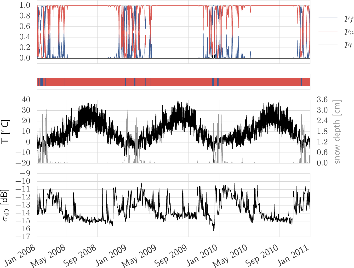
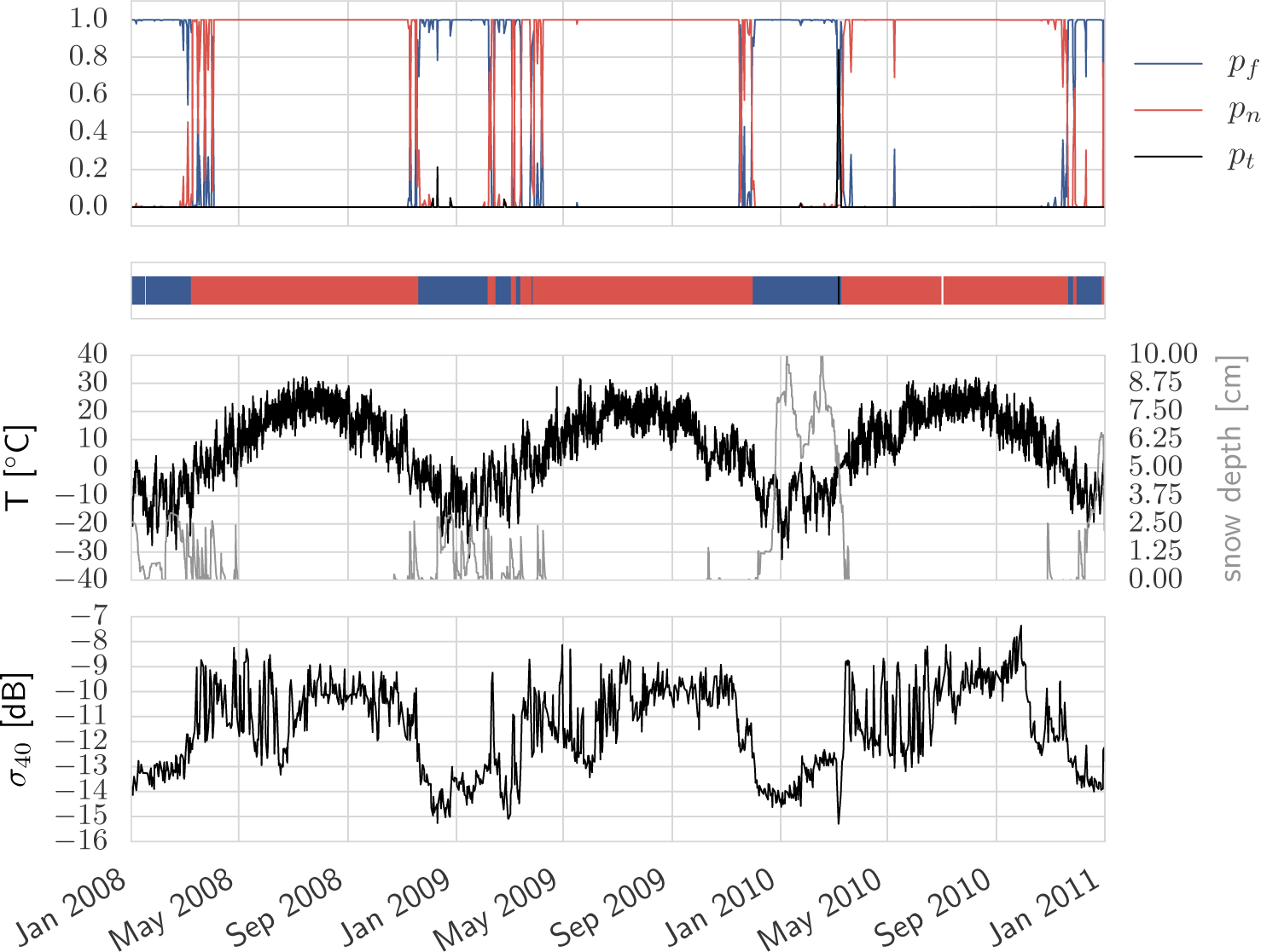
Three examples of the inferred F/T (using the full HMMFT model) state in different temperate climatic regions within the USA are shown in Figures 1–3, and the agreements with both ERA Interim and in situ-derived F/T states are summarized in Table 3. The winters in the first one, Orchard Range in Figure 1, are characterized by intermittent snow cover (maximum height of around 3 cm) and frequent, often diurnal changes between below and above zero temperatures. This is reflected in the inferred F/T state (overall agreement with in situ data: 86%); in summer, by way of contrast, the temperatures remain above the freezing point for months. The backscatter during the summer months is dominated by the variations in soil moisture (these are not shown in the figure) due to precipitation and evaporation.
The second station in South Dakota (Figure 2) is at almost the same latitude, but further to the east; the dry winters are colder with longer periods (of several weeks) of subzero temperatures and, thus, predominantly frozen conditions. These are reflected in the backscatter time series, which displays an offset of about 5 dB between winter and summer.
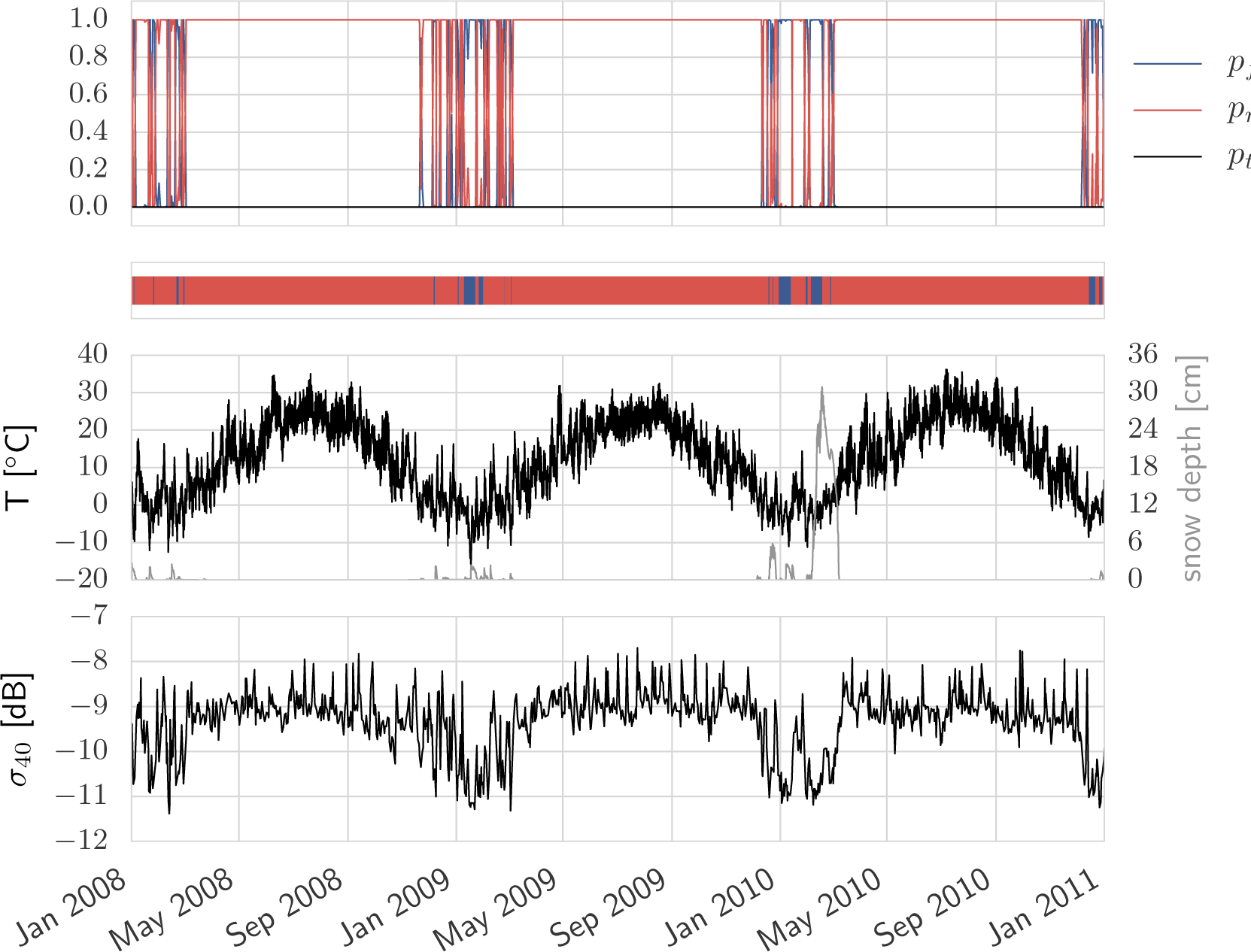
Even further to the east in Pennsylvania (Figure 3), the climate and, with it, the winters become more humid and warmer: the periods of temperatures below freezing are reduced, and during these, diurnal changes to above-zero temperatures are common. These changes are evident in the inferred F/T state (overall agreement with in situ data: 90%), as well as the backscatter data. Despite the warmer temperatures, larger snow covers can accumulate (30 cm depth in early spring 2010). During the melting of the snow, no distinct drop in σ40 is discernible.
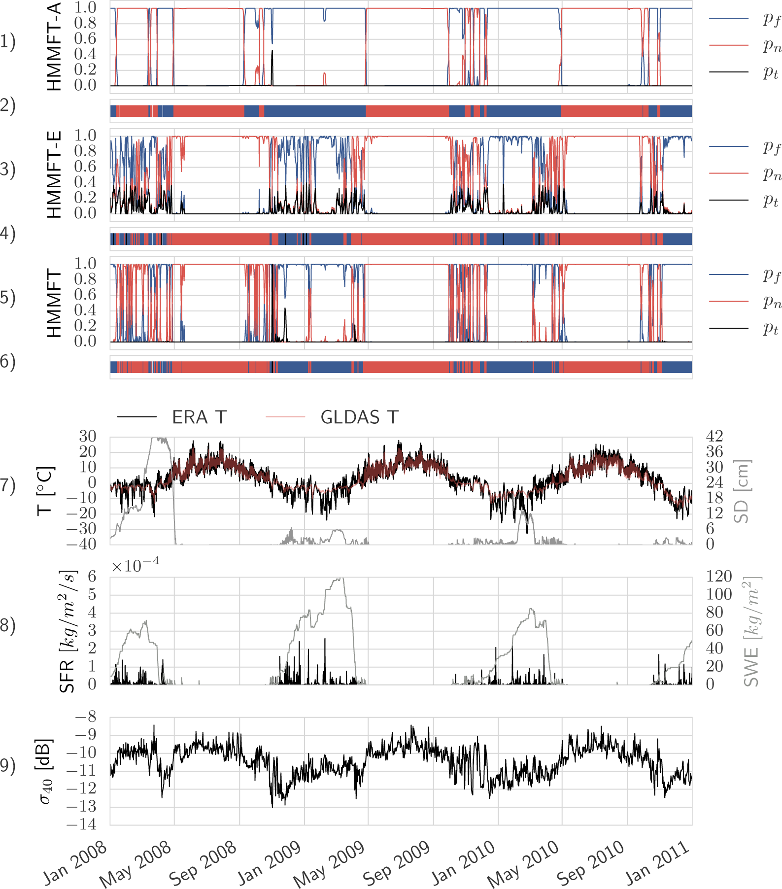
The F/T time series in Sweden (Figure 4) shows a number of such drops, e.g., in November, 2008: the ASCAT-only F/T State (HMMFT-A) attaches a posterior probability > 0.4 to the first one in the first week of November, but one < 0.01 to the second at the end of November, whereas the one based on both temperature and backscatter data assigns one exceeding 0.4 to both events. The ERA Interim snow data indicate no presence of snow on the first day (as opposed to the GLDAS record, which suggests melting snow), but a partial melting event on the second. The melting of snow does not always lead to a drop in backscatter [47,48], such as in April, 2010.
5.1.2. Maps
Figure 5 presents the average a posteriori probability of frozen conditions in the months of March to June, 2007: the successive poleward shift of the boundary between the predominantly frozen and non-frozen regions is evident in the Northern Hemisphere, with some exceptions in mountainous regions.
5.2. Comparison with External Data
The accuracy of the proposed algorithm (HMMFT) and the Surface State Flag (SSF) can be assessed and compared with respect to the three external datasets: GLDAS ST, ISMN ST and WMO AT.
5.2.1. GLDAS ST
The agreement of Equation (6) with respect to the GLDAS F/T state aHMMFT;GLDAS is summarized on a global basis in Table 4; these results are grouped according to different times of year, whose temporal extent depends on the location and is defined in detail in [16]. They are: winter, the transition period between winter and summer (TWS, duration: 60 days), summer and the transition between summer and winter (TSW, duration: 60 days).
The accuracy of the HMMFT exceeds the one of the SSF for all seasons for this dataset, with the difference being particularly pronounced in the transition to summer TWS (difference of 14.1 percentage point). The overall accuracy is also larger: 92.6 for HMMFT, 83.9 for SSF.
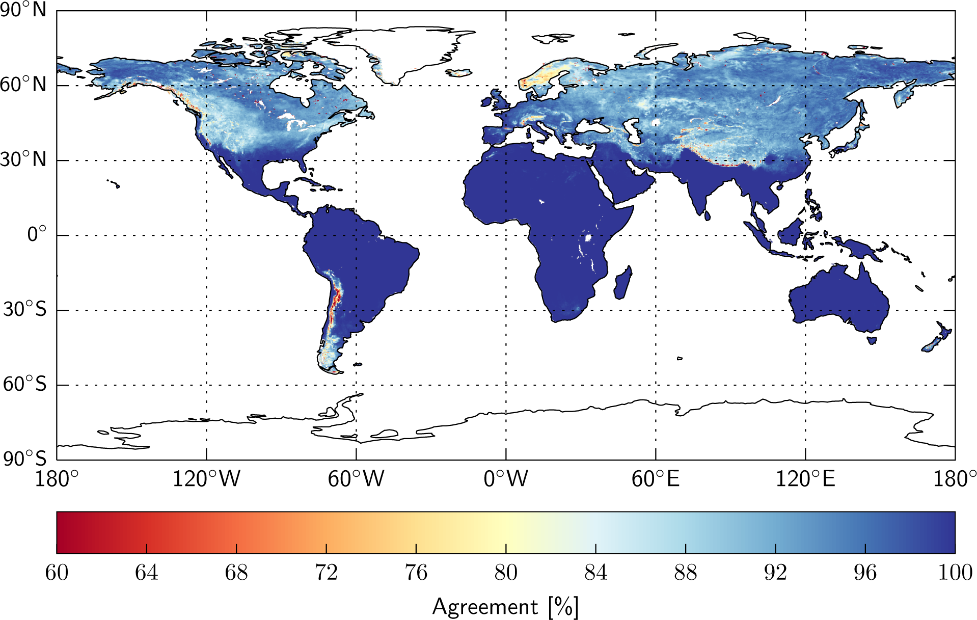
The global mean of the agreement aHMMFT;GLDAS averaged over all seasons is 95.5%; the latter’s spatial distribution is shown in Figure 6. Areas with aHMMFT;GLDAS > 95%, depicted in dark blue, are prevalent where freezing temperatures are exceedingly rare. In the remaining regions, typical values of 85%–95% dominate. Exceptions include Scandinavia and several mountain ranges, such as the Andes.
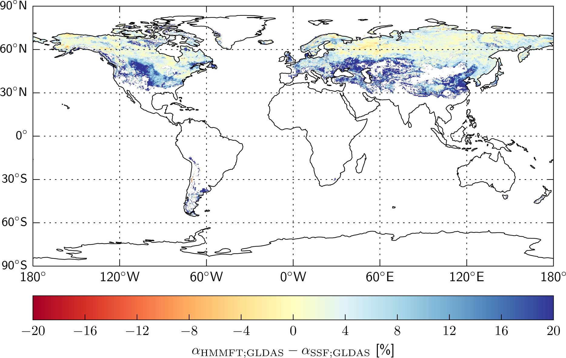
How these values compare to the SSF is visualized in Figure 7, where aHMMFT;GLDAS − aSSF;GLDAS is mapped. In the areas north of 55°N, this difference is smaller than five percentage points (pp) in magnitude, but in more temperate regions (e.g., Eastern Europe, Central Asia), aHMMFT;GLDAS can exceed aSSF;GLDAS by more than 10 percentage points (pp). The figure shows areas where the SSF does not produce a valid result in white, since no comparison could be made.
5.2.2. WMO AT
The comparison with the WMO air temperature data is summarized in Table 5: despite the different kind of reference data and the scale mismatch, the results are also broadly similar to the comparison with GLDAS ST. The HMMFT exhibits higher agreements than the SSF in all periods, with the greatest difference occurring in the transition seasons (aHMMFT;GLDAS − aSSF;GLDAS > 13 pp); overall, it is 10.2 pp.
5.2.3. ISMN Soil Temperature
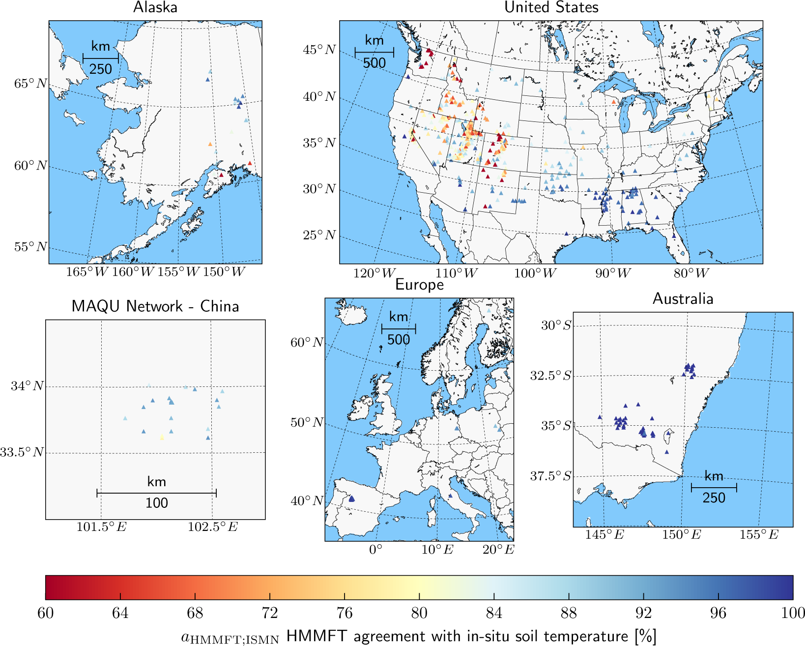
Unlike the previous external datasets, the measurements of some in situ soil temperature sensors do not necessarily cover the entire year; cf. Section 2. The agreement with these ST values is shown in Figure 8 and summarized (grouped according to the soil moisture networks) in Table 6. Both the annual means, as well as the respective differences between HMMFT and SSF are broadly consistent with the previous two datasets. Furthermore, the comparatively low accuracies obtained over some mountainous areas are reflected in the ISMN ST results: they are even more pronounced in some stations of the Soil Climate Analysis Network (SCAN) and Snow Telemetry (SNOTEL) networks (aHMMFT;ISMN < 60%), with conspicuous effects on the mean agreements in Table 6.
5.3. Sensitivity Analyses
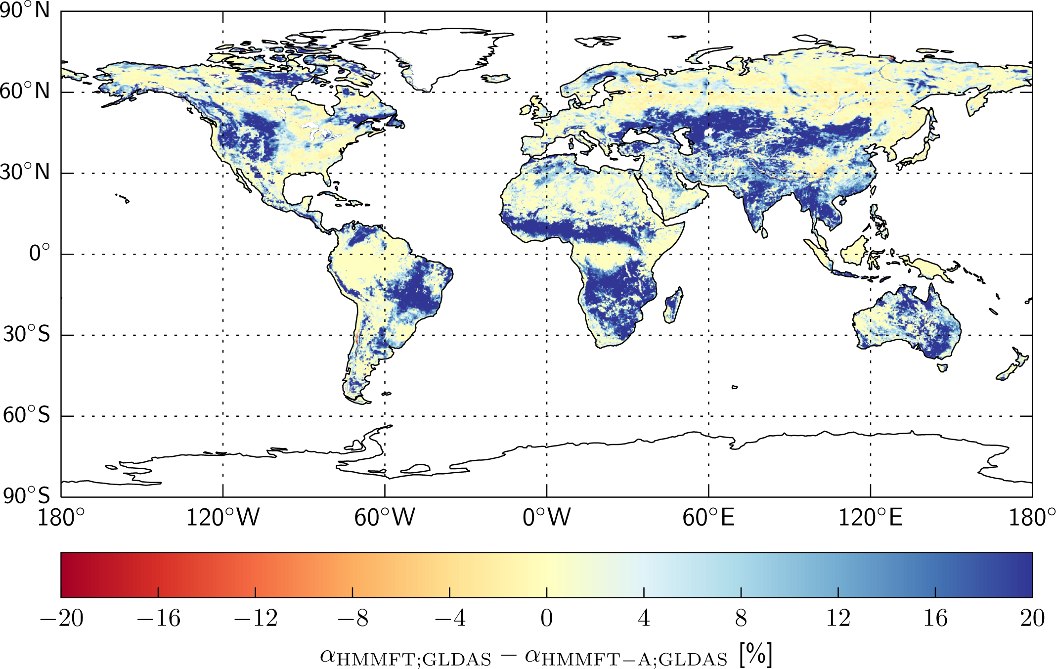
In contrast to the SSF, the HMMFT algorithm relies on both radar (ASCAT) and temperature (ERA Interim) as input data. The relative importance of these two datasets can be gauged from the agreement of the two sensitivity model runs with GLDAS ST. The change in agreement when the temperature data are left out (ASCAT-only; HMMFT-A) is limited (|aHMMFT;GLDAS − aHMMFT−A;GLDAS| < 5 pp) in parts of Eurasia (in particular, north of 55°), but also some regions in the tropics (e.g., Amazon rain forest) or the SE United States; see Figure 9. Decreases in accuracy exceeding 10 pp are widespread: they occur in, e.g., Central Asia and southern Africa, frequently where the SSF attains comparatively low accuracies (see Figure 7).
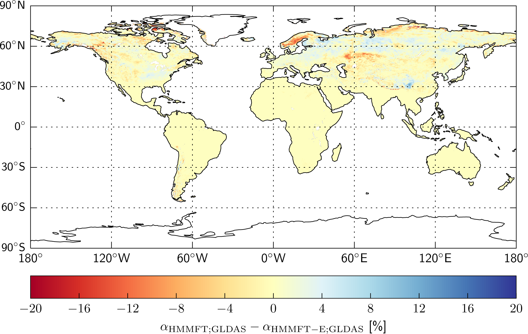
The difference to the ERA Interim-only version HMMFT-E is less than 5 pp in most parts of the world (Figure 10), with both versions achieving similar accuracies, except in a few regions; the difference is particularly pronounced in Scandinavia, where aHMMFT;GLDAS − aHMMFT−E;GLDAS < 10 pp.
6. Discussion
6.1. Quality Assessment
6.1.1. Temporal Analysis
The mismatch between the inferred F/T state and the one obtained from external data is seen to vary during the year: the agreements tend to be lower during the transition periods than during either summer or winter; cf. Tables 4 and 5. This pattern pertains to both the proposed HMM algorithm and the previously published SSF. The higher agreement for the HMM persists across both external datasets and all seasons; it is particularly pronounced during the transition periods TWS and TSW.
This tendency has been previously observed in numerous studies, e.g., [16,22,39]. For many scientific purposes, such as the monitoring of the length of the growing season [12,25] or the onset of snow melt [8], these transition periods are of crucial importance and also the periods where remote sensing data can prove particularly useful. The information they provide during these periods is quite distinct from what can be inferred from temperature measurements alone, which might also contribute to the observed discrepancies. For the purpose of flagging measurements for soil moisture retrieval, the winter and summer periods are at least as important, as any prolonged misclassification during these is expected to have a large impact on the quality.
6.1.2. Spatial Analysis
The areal comparison with ISMN in situ station data in Figure 8 shows that only low accuracies are obtained in the Rocky Mountains and the coastal mountain ranges of North America. The assessment with GLDAS data in Figure 7 is consistent in these areas and also shows low agreements in other mountainous areas, such as the Ural, as well as parts of Scandinavia. The latter figure shows that the SSF algorithm is plagued by similar problems (as are other approaches [48]) and achieves even lower accuracies in the aforementioned regions. Overall, the HMM scheme tends to have better correspondences in most parts of the world, except for certain regions in northwest Asia and Alaska.
6.2. Remote Sensing and Temperature-Based F/T States
These accuracy measures are, like in many previous studies [8,12], based on F/T states derived from temperature measurements. These temperature proxies are indicative of, but not necessarily equivalent to the radar F/T state [11,22,49]; some of the factors that contribute to this lack of representativeness for flagging backscatter measurements are as follows.
6.2.1. Snow Wetness
The properties of wet snow in the microwave region (e.g., scattering and absorption) differ noticeably from snow-free conditions; they thus have to be flagged for reliable soil moisture retrieval. The drop in backscatter associated with increasing liquid water content in snow has led to the inclusion of the state t [22]. However, the relation between the liquid water content of snow and both the air temperature above and the soil temperature below the snowpack is not clear-cut. Thus, the state t has not been considered when assessing F/T retrievals by temperature measurements [8]. In addition, it is only crudely considered in the estimated parameterization of the transition probabilities of Section 3.2, in that positive temperatures close to the freezing point favor the switch to t from f. However, they also enable a transition to n, and it is thus the backscatter information that will govern the inferred F/T state. An example of an estimated F/T state t can be found during the snow melt in March, 2010, in Figure 2.
6.2.2. Spatial Representativeness
Both the WMO and ISMN measurements are representative of horizontal scales with a typical extension of a few meters; the GLDAS and ASCAT data, on the other hand, to dozens of kilometers. This mismatch is expected to be particularly pronounced in topographically complex regions [16], as both the snow cover and the temperature distribution typically depends on altitude and slope aspect. This could affect the time series in Idaho (located at the foot of a mountain range) in Figure 1 and also explain the lower agreements found in mountain ranges, in particular with the ISMN ST in the Rocky Mountains; see Figures 6 and 8.
This topographic complexity has recently been studied with respect to its scale dependence by [50] and [30], who detected an influence of both altitude and aspect of the slopes. They also analyzed the impact of heterogeneous land cover, which was found to be frequency dependent. Such frequency dependence is expected to be not only due to the vegetation and snow cover [22,40], but has also been observed over bare soil. Wegmuller [51] found different scattering behavior as a function of the depth of the frozen layer above thawed soil, as well as for the inverse situation.
6.2.3. Temperature Data
The evolution of the temperature of the air and the top soil is tightly coupled [41]; however, due to, e.g., limited heat transport (relevant parameters include the soil heat conductivity and the boundary layer structure) and changes in internal energy (phase or temperature change), they are not expected to be equal at any one point in time. Simple physical diffusion models consider the air temperature as the driving term, such that the soil temperature is a low-pass filtered version; this rationale is reflected in the transition probabilities of the HMM. The most pronounced differences between the two temperatures are thus expected in the presence of high-frequency variations in air temperatures, e.g., during the transition seasons or during diurnal F/T cycles. The associated discrepancy of the different temperature proxies and the radar F/T state has been observed in both this study (e.g., Tables 4 and 5) and previous ones [16,22,39].
The physical temperature is closely related to the state of the water present in the landscape. The amount of frozen or liquid water in vegetation and soil as a function of temperature depends on several factors (such as the soil texture and the concentration of dissolved substances). Different functional relationships have been suggested, and hysteresis has been observed, e.g., [41]. The term F/T state and the commonly employed assessment approaches belie this immanent complexity: they rather assume that it is a binary decision whether a particular radar observation is affected, and the latter additionally assert that this decision can be made on the basis of a temperature measurement. The choice of these thresholds thus also varies in the relevant literature, e.g., [16,22]. This abrupt temperature dependence of the F/T state can lead to a high sensitivity to errors in the input temperature data, the accuracy of which in models depends, amongst other factors, on the density of ground stations, which is comparatively low in many subarctic regions [41].
6.3. Relative Importance of ASCAT and ERA Interim Data
This intrinsic discrepancy between temperature-based and remotely-sensed F/T states is also pertinent to the comparison of the partial input versions of the HMM, whose inclusion serves the purpose of analyzing the relative importance of the ASCAT and ERA Interim data. As the model run based exclusively on temperature data is compared to F/T states based exclusively on temperature data, as well, the agreement might be expected to be comparatively large.
Despite these difficulties in assessing the results of the partial input versions, a central question can still be addressed: are both ERA Interim and ASCAT data necessary?
The contribution of the ERA Interim dataset is made evident in Figure 9, which shows an increase in agreement with GLDAS ST compared to the ASCAT-only version exceeding 15 pp in many parts of the world, e.g., Southern Africa, Central Asia and the Amazon rain forest. Its importance in deriving the F/T state for C-band radar, in particular in regions where freezing conditions are rare, has also been observed by [16] and is also evident in Figure 2.
The relevance of the ASCAT data is more difficult to assess, as it is expected to be particularly large during those conditions, where the comparison with proxy F/T states is known to be inadequate, such as during diurnal F/T cycles (e.g., Figure 3) or the presence of wet snow (e.g., Figure 2). In the latter case, the inference of state t is mostly governed by the backscatter; see Section 6.2 and Figure 4. The latter also gives an example of the difference between HMMFT-E and HMMFT-A during periods of diurnal freeze thaw cycling, such as in April, 2010: the backscatter is on the level of the preceding months (i.e., winter conditions), but the HMMFT-E indicates thawed conditions, as the ERA Interim temperatures are on average above the freezing point. The opposite behavior is observed in the previous autumn (October, 2009): the backscatter exhibits large fluctuation, but is on average similar to the one of the preceding winter, such that the HMMFT-A infers frozen conditions, whereas the HMMFT (due to the inclusion of temperature data) points towards numerous changes between frozen and non-frozen conditions.
6.4. Comparison with the SSF
The combined algorithm HMMFT, using both temperature and backscatter data, achieves consistently higher accuracies than the SSF; cf. Section 5.2. The agreement with GLDAS ST is particularly increased in areas between 30 and 50°N, where thawed conditions are frequent and, thus, soil moisture information relevant for monitoring the hydrologic cycle. For this purpose, it is also important that, as opposed to the SSF, the HMM algorithm can always produce an F/T state. This F/T state is given in terms of probabilities, which implies that one can (or has to) choose appropriate thresholds on the probabilities to flag backscatter measurements for soil moisture retrieval.
7. Conclusions
Frozen conditions have a profound impact on the interaction of the soil and vegetation cover with microwaves. They thus impede the estimation of soil moisture based on both passive and active microwave remote sensing techniques. The Advanced Scatterometer (ASCAT) instruments are such active microwave sensors, and they provide data from which a global soil moisture product is derived. This product requires an accurate detection of frozen conditions. The proposed algorithm is the first one to be based on a probabilistic time series model that incorporates both ASCAT backscatter measurements and reanalysis air temperature data. The former are the observations whose distribution depends on the freeze/thaw (F/T) state; the latter serve as a generalized forcing term that governs the temporal evolution of the F/T state. The inclusion of air temperature is found to be particularly relevant in regions where frozen conditions are not common, as it leads to improved agreements (more than 10 pp) with externally-derived freeze/thaw detections. The suggested approach also consistently achieves higher agreements with reference datasets than the currently used algorithm for ASCAT freeze/thaw detection, which does not incorporate simultaneous temperature data. These assessments are fraught with difficulties and inconsistencies, as they do not compare like with like, but the results do indicate that the new method is more robust, as it is applicable at all grid points. Despite the considerably larger computational burden, the global applicability makes it a suitable algorithm for the purpose of screening the ASCAT backscatter observations used in soil moisture retrieval. The impact of such screening will be greater where freezing occurs regularly, such as in hemiboreal and subarctic climates. Particularly in these regions, the improved estimation of soil moisture and the freeze/thaw state is thus expected to contribute to the monitoring of land surface processes and changes.
Acknowledgments
The authors acknowledge the support of the Austrian Space Application Programme (ASAP) through the GMSM (Global Monitoring of Soil Moisture for Water Hazards Assessment) project, of the European Space Agency (ESA) through the Climate Change Initiative (CCI) Soil Moisture project and of the 7th Framework Program through the Geoland2 project (Project 218795).
- Author ContributionsSimon Zwieback and Wolfgang Wagner conceived of and designed the study. Christoph Paulik and Simon Zwieback implemented the algorithm and processed the data. All three authors interpreted the results and wrote the manuscript.
- Conflicts of InterestThe authors declare no conflict of interest.
References
- Naeimi, V.; Scipal, K.; Bartalis, Z.; Hasenauer, S.; Wagner, W. An Improved Soil Moisture Retrieval Algorithm for ERS and METOP Scatterometer Observations. IEEE Trans. Geosci. Remote Sens. 2009, 47, 1999–2013. [Google Scholar]
- Wagner, W.; Hahn, S.; Kidd, R.; Melzer, T.; Bartalis, Z.; Hasenauer, S.; Figa-Saldaña, J.; de Rosnay, P.; Jann, A.; Schneider, S.; et al. The ASCAT Soil Moisture Product: A Review of its Specifications, Validation Results and Emerging Applications. Meteorol. Z 2013, 22, 5–33. [Google Scholar]
- Woodhouse, I.H.; Hoekman, D. Determining Land-Surface Parameters from the ERS Wind Scatterometer. IEEE Trans. Geosci. Remote Sens. 2000, 38, 126–140. [Google Scholar]
- Macelloni, G.; Paloscia, S.; Pampaloni, P.; Ruisi, R.; Dechambre, M.; Valentin, R.; Chanzy, A.; Wigneron, J.P. Active and passive microwave measurements for the characterization of soils and crops. Agronomie 2002, 22, 581–586. [Google Scholar]
- Zribi, M.; le Hegarat-Mascle, S.; Ottle, C.; Kammoun, B.; Guerin, C. Surface soil moisture estimation from the synergistic use of the (multi-incidence and multi-resolution) active microwave ERS Wind Scatterometer and SAR data. Remote Sens. Environ. 2003, 86, 30–41. [Google Scholar]
- Pellarin, T.; Calvet, J.C.; Wagner, W. Evaluation of ERS scatterometer soil moisture products over a half-degree region in southwestern France. Geophys. Res. Lett. 2006, 33. [Google Scholar] [CrossRef]
- Draper, C.; Mahfouf, J.; Calvet, J.; Martin, E.; Wagner, W. Assimilation of ASCAT near-surface soil moisture into the SIM hydrological model over France. Hydrol. Earth Syst. Sci. 2011, 15, 3829–3841. [Google Scholar]
- Bartsch, A.; Kidd, R.; Wagner, W.; Bartalis, Z. Temporal and spatial variability of the beginning and end of daily spring freeze/thaw cycles derived from scatterometer data. Remote Sens. Environ. 2007, 106, 360–374. [Google Scholar]
- Wang, L.; Derksen, C.; Brown, R. Detection of pan-Arctic terrestrial snowmelt from QuikSCAT, 2000–2005. Remote Sens. Environ. 2008, 112, 3794–3805. [Google Scholar]
- Zhao, T.; Zhang, L.; Jiang, L.; Zhao, S.; Chai, L.; Jin, R. A new soil freeze/thaw discriminant algorithm using AMSR-E passive microwave imagery. Hydrol. Process. 2011, 25, 1704–1716. [Google Scholar]
- Bartsch, A.; Kumpula, T.; Forbes, B.; Stammler, S. Detection of Snow Surface Thawing and Refreezing in the Eurasian Arctic Using QuikSCAT: Implications for Reindeer Herding. Ecol. Appl. 2010, 20, 2346–2358. [Google Scholar]
- Kimball, J.; McDonald, K.; Running, S.; Frolking, S. Satellite radar remote sensing of seasonal growing seasons for boreal and subalpine evergreen forests. Remote Sens. Environ. 2004, 90, 243–258. [Google Scholar]
- Jones, M.; Kimball, J.; Jones, L.; McDonald, K. Satellite passive microwave detection of North America start of season. Remote Sens. Environ. 2012, 123, 324–333. [Google Scholar]
- Bartsch, A.; Wagner, W.; Rupp, K.; Kidd, R. Application of C and Ku-Band Scatterometer Data for Catchment Hydrology in Northern Latitudes, Proceedings of the 2007 IEEE International Geoscience and Remote Sensing Symposium (IGARSS 2007), Barcelona, Spain, 23–28 July 2007; pp. 3702–3705.
- Kim, Y.; Kimball, J.; McDonald, K.C.; Glassy, J. Developing a Global Data Record of Daily Landscape Freeze/Thaw Status Using Satellite Passive Microwave Remote Sensing. IEEE Trans. Geosci. Remote Sens. 2011, 49, 949–960. [Google Scholar]
- Naeimi, V.; Paulik, C.; Bartsch, A.; Wagner, W.; Member, S.; Kidd, R.; Park, S.E.; Elger, K.; Boike, J. ASCAT Surface State Flag (SSF): Extracting Information on Surface Freeze/Thaw Conditions From Backscatter Data Using an Empirical Threshold-Analysis Algorithm. IEEE Trans. Geosci. Remote Sens. 2012, 50, 2566–2581. [Google Scholar]
- Entekhabi, D.; Njoku, E.; O’Neill, P.; Kellogg, K.; Crow, W.; Edelstein, W.; Entin, J.; Goodman, S.; Jackson, T.; Johnson, J.; et al. The Soil Moisture Active Passive SMAP Mission. Proc. IEEE. 2010, 98, 704–716. [Google Scholar]
- Owe, M.; de Jeu, R.; Holmes, T. Multisensor historical climatology of satellite-derived global land surface moisture. J. Geophys. Res. 2008, 113. [Google Scholar] [CrossRef]
- Bartsch, A.; Sabel, D.; Wagner, W.; Park, S.E. Considerations for derivation and use of soil moisture data from active microwave satellites at high latitudes 3132–3135.
- Bartsch, A.; Duguay, C.; Heim, B.; Strozzi, T.; Urban, M.; Wiesmann, A.; Sabel, D.; Naeimi, V.; Paulik, C.; Ressl, J; et al. Final Report v2. ESA DUE Permafrost Deliverable 19, 2012. Available online: http://geo.tuwien.ac.at/permafrost/index.php/publications/final-report accessed on 17 March 2015.
- Högström, E.; Trofaier, A.M.; Gouttevin, I.; Bartsch, A. Assessing seasonal backscatter variations with respect to uncertainties in soil moisture retrieval in Siberian Tundra regions. Remote Sens. 2014, 6, 8718–8738. [Google Scholar]
- Zwieback, S.; Bartsch, A.; Melzer, T.; Wagner, W. Probabilistic fusion of Ku and C band scatterometer data for determining the freeze/thaw state. IEEE Trans. Geosci. Remote Sens. 2012, 50, 2583–2594. [Google Scholar]
- Mooney, P.; Mulligan, F.; Fealy, R. Comparison of ERA-40, ERA-Interim and NCEP/NCAR reanalysis data with observed surface air temperatures over Ireland. Int. J. Climatol. 2011, 31, 545–557. [Google Scholar]
- Wang, S.; Zhang, M.; Sun, M.; Wang, B.; Huang, X.; Wang, Q.; Feng, F. Comparison of surface air temperature derived from NCEP/DOE R2, ERA-Interim, and observations in the arid northwestern China: a consideration of altitude errors. Theor. Appl. Climatol. 2015, 119, 99–111. [Google Scholar]
- Kimball, J.; McDonald, K.; Frolking, S.; Running, S. Radar remote sensing of the spring thaw transition across a boreal landscape. Remote Sens. Environ. 2004, 89, 163–175. [Google Scholar]
- Jin, R.; Li, X.; Che, T. A decision tree algorithm for surface soil freeze/thaw classification over China using SSM/I brightness temperature. Remote Sens. Environ. 2009, 113, 2651–2660. [Google Scholar]
- Figa-Saldaña, J.; Wilson, J.; Attema, E.; Gelsthorpe, R.; Drinkwater, M.; Stoffelen, A. The advanced scatterometer (ASCAT) on the meteorological operational (MetOp) platform: A follow on for European wind scatterometers. Can. J. Remote Sens. 2002, 28, 404–412. [Google Scholar]
- Berrisford, P.D.D.; Fielding, K.; Fuentes, M.; Kållberg, P.; Kobayashi, S.; Uppala, S. The ERA-Interim Archive; ERA Report Series 1; ECMWF: Reading, UK, 2009; p. 16. [Google Scholar]
- Kerr, Y.; Waldteufel, P.; Richaume, P.; Wigneron, J.P.; Ferrazzoli, P.; Mahmoodi, A.; Al Bitar, A.; Cabot, F.; Gruhier, C.; Juglea, S.E.; et al. The SMOS Soil Moisture Retrieval Algorithm. IEEE Trans. Geosci. Remote Sens. 2012, 50, 1384–1403. [Google Scholar]
- Podest, E.; McDonald, K.C.; Kimball, J. Multisensor Microwave Senstivity to Freeze/Thaw Dynamics Across a Complex Boreal Landscape. IEEE Trans. Geosci. Remote Sens. 2014, 52, 6818–6829. [Google Scholar]
- Rodell, M.; Houser, P.R.; Jambor, U.; Gottschalck, J.; Mitchell, K.; Meng, C.; Arsenault, K.; Cosgrove, B.; Radakovich, J.; Bosilovich, M.; et al. The Global Land Data Assimilation System. Bull. Am. Meteorol. Soc. 2004, 85, 381–394. [Google Scholar]
- Ek, M.; Mitchell, K.; Lin, Y.; Rogers, E.; Grunmann, P.; Koren, V.; Gayno, G.; Tarpley, J. Implementation of the upgraded Noah land-surface model in the NCEP operational mesoscale Eta model. J. Geophys. Res. 2003, 108. [Google Scholar] [CrossRef]
- Dorigo, W.; Xaver, A.; Vreugdenhil, M.; Gruber, A.; Hegyiova, A.; Sanchis-Dufau, A.; Zamojski, D.; Cordes, C.; Wagner, W.; Drusch, M. Global automated quality control of in-situ soil moisture data from the International Soil Moisture Network. Vadose Zone J 2013. [Google Scholar] [CrossRef]
- Dorigo, W.; Wagner, W.; Hohensinn, R.; Hahn, S.; Paulik, C.; Xaver, A.; Gruber, A.; Drusch, M.; Mecklenburg, S.; van Oevelen, P.; et al. The International Soil Moisture Network: A data hosting facility for global in situ soil moisture measurements. Hydrol. Earth Syst. Sci. 2011, 15, 1675–1698. [Google Scholar]
- Gruber, A.; Dorigo, W.; Zwieback, S.; Xaver, A.; Wagner, W. Characterizing Coarse-Scale Representativeness of in situ Soil Moisture Measurements from the International Soil Moisture Network. Vadose Zone J 2013. [Google Scholar] [CrossRef]
- WMO. DS512.0 Data Hosting Facility, 2011, Available online: http://rda.ucar.edu/datasets/ds512.0/ accessed on 17 March 2015.
- Holmes, T.R.H.; Crow, W.T.; Hain, C. Spatial patterns in timing of the diurnal temperature cycle. Hydrol. Earth Syst. Sci. Discuss. 2013, 10, 6019–6048. [Google Scholar]
- McDonald, K.; Zimmermann, R.; Kimball, J. Diurnal and spatial variation of xylem dielectric constant in Norway Sruce (Picea abies [L.] Karst.) as related to microclimate, xylem sap flow and xylem chemistry. IEEE Trans. Geosci. Remote Sens. 2002, 40, 2063–2082. [Google Scholar]
- Wismann, V. Monitoring of Seasonal Thawing in Siberia with ERS Scatterometer Data. IEEE Trans. Geosci. Remote Sens. 2000, 38, 1804–1809. [Google Scholar]
- Colliander, A.; McDonald, K.; Zimmermann, R.; Schroeder, R.; Kimball, J.; Njoku, E.G. Application of QuikSCAT Backscatter to SMAP Validation Planning: Freeze/Thaw State Over ALECTRA Sites in Alaska From 2000 to 2007. IEEE Trans. Geosci. Remote Sens. 2012, 50, 461–469. [Google Scholar]
- Viterbo, P.; Beljaars, A.; Mahfouf, J.; Teixeira, J. The representation of soil moisture freezing and its impact on the stable boundary layer. Q. J. R. Meteorol. Soc. 1999, 125, 2401–2426. [Google Scholar]
- Lewis, P.; Gomez-Dans, J.; Kaminski, T.; Settle, J.; Quaife, T.; Gobron, N.; Styles, J.; Berger, M. An Earth Observation Land Data Assimilation System (EO-LDAS). Remote Sens. Environ. 2012, 120, 219–235. [Google Scholar]
- Wolfe, P. Convergence conditions for ascent methods. SIAM Rev. 1969, 11, 226–235. [Google Scholar]
- Ruppert, D. Statistics and Data Analysis for Financial Engineering; Springer: New York, NY, USA, 2011. [Google Scholar]
- Ashcraft, I.; Long, D. Comparison of methods for melt detection over Greenland using active and passive microwave measurements. Int. J. Remote Sens. 2006, 27, 2469–2488. [Google Scholar]
- Barber, D.; Taylan, C. Graphical Models for Time Series. IEEE Signal Process. Mag. 2010, 27, 18–28. [Google Scholar]
- Wagner, W.; Walker, A.; Helmut, R. Application of Low-Resolution Active Microwave Remote Sensing (C-Band) Over the Canadian Prairies, Proceedings of the 17th Canadian Symposium on Remote Sensing, Saskatoon, Saskatchewan, Canada, 13–15 June 1995; pp. 21–28.
- Park, S.E.; Bartsch, A.; Sabel, D.; Wagner, W.; Naeimi, V.; Yamaguchi, Y. Monitoring freeze/thaw cycles using ENVISAT ASAR Global Mode. Remote Sens. Environ. 2011, 115, 3457–3467. [Google Scholar]
- Colliander, A.; McDonald, K.; Zimmerman, R.; Podest, E.; Schroeder, R.; Kimball, J.; Njoku, E. Active and Passive multi-scale microwave remote sensing of the Alaska Ecological Transect: Application to SMAP freeze/thaw state validation planning, Proceedings of the International Geoscience and Remote Sensing Symposium (IGARSS), Vancouver, Canada, 24–29 July 2011; pp. 3156–3159.
- Du, J.; Kimball, J.S.; Azarderakhsh, M.; Dunbar, R.S.; Moghaddam, M.; McDonald, K.C. Classification of Alaska Spring Thaw Characteristics Using SatelliteL-Band Radar Remote Sensing. IEEE Trans. Geosc. Remote Sens. 2015, 53, 542–556. [Google Scholar]
- Wegmüller, U. The effect of freezing and thawing on the microwave signatures of bare soil. Remote Sens. Environ. 1990, 33, 123–135. [Google Scholar]


| μt = μf − 3 | bt =bf |
| Flag | Frozen | Unfrozen | |
|---|---|---|---|
| Temperature | < 0 °C | correct (TP) | incorrect (FN) |
| > 0 °C | incorrect (FP) | correct (TN) | |
| Invalid | % of unknown or not valid flags | ||
| Station | ERA Interim | In Situ |
|---|---|---|
| Orchard Range | 93.05 | 85.77 |
| Eros Data Center | 95.13 | 89.98 |
| Mahantango Creek | 94.76 | 90.63 |
| Winter | TWS | Summer | TSW | Overall | |
|---|---|---|---|---|---|
| HMMFT | 93.5 | 82.7 | 97.9 | 86.4 | 92.6 |
| SSF | 88.2 | 68.6 | 91.4 | 75.1 | 83.9 |
| Winter | TWS | Summer | TSW | Overall | |
|---|---|---|---|---|---|
| HMMFT | 87.5 | 85.8 | 98.6 | 88.7 | 92.1 |
| SSF | 77.9 | 71.7 | 92.3 | 73.4 | 81.9 |
| Network | Full name | Time Series(l/nl) | aSSF(l);ISMN | aHMMFT(l);ISMN | aHMMFT(nl);ISMN |
|---|---|---|---|---|---|
| ARM | Atmospheric Radiation Measurement | 37/12 | 76.35 | 89.90 | 80.98 |
| FLUXNET-AMERIFLUX | FLUXNET AmeriFlux | 0/4 | – | – | 99.96 |
| FMI | Finnish Meteorological Institute | 2/0 | 81.49 | 88.78 | – |
| HYDROL-NET_PERUGIA | Hydrological network Perugia | 1/0 | 85.42 | 97.96 | – |
| ICN | Illinois Climate Network | 1/0 | 83.00 | 89.31 | – |
| MAQU | Maqu | 15/5 | 89.84 | 89.67 | 89.69 |
| MOL-RAO | Meteorological Observatory Lindenberg | 2/0 | 85.96 | 94.26 | – |
| REMEDHUS | Remedhus | 20/0 | 69.13 | 99.08 | – |
| SCAN | Soil Climate Analysis Network | 124/156 | 77.17 | 90.30 | 84.38 |
| SNOTEL | Snow Telemetry | 124/180 | 69.25 | 79.25 | 74.21 |
| SWEX_POLAND | Soil, Water And Energy Exchange Poland | 4/0 | 82.01 | 91.78 | – |
| USDA-ARS | United States Department of Agriculture | 4/4 | 67.20 | 91.67 | 96.79 |
© 2015 by the authors; licensee MDPI, Basel, Switzerland This article is an open access article distributed under the terms and conditions of the Creative Commons Attribution license (http://creativecommons.org/licenses/by/4.0/).
Share and Cite
Zwieback, S.; Paulik, C.; Wagner, W. Frozen Soil Detection Based on Advanced Scatterometer Observations and Air Temperature Data as Part of Soil Moisture Retrieval. Remote Sens. 2015, 7, 3206-3231. https://doi.org/10.3390/rs70303206
Zwieback S, Paulik C, Wagner W. Frozen Soil Detection Based on Advanced Scatterometer Observations and Air Temperature Data as Part of Soil Moisture Retrieval. Remote Sensing. 2015; 7(3):3206-3231. https://doi.org/10.3390/rs70303206
Chicago/Turabian StyleZwieback, Simon, Christoph Paulik, and Wolfgang Wagner. 2015. "Frozen Soil Detection Based on Advanced Scatterometer Observations and Air Temperature Data as Part of Soil Moisture Retrieval" Remote Sensing 7, no. 3: 3206-3231. https://doi.org/10.3390/rs70303206