
Toward Estimating Wetland Water Level Changes Based on Hydrological Sensitivity Analysis of PALSAR Backscattering Coefficients over Different Vegetation Fields


Abstract
:
1. Introduction
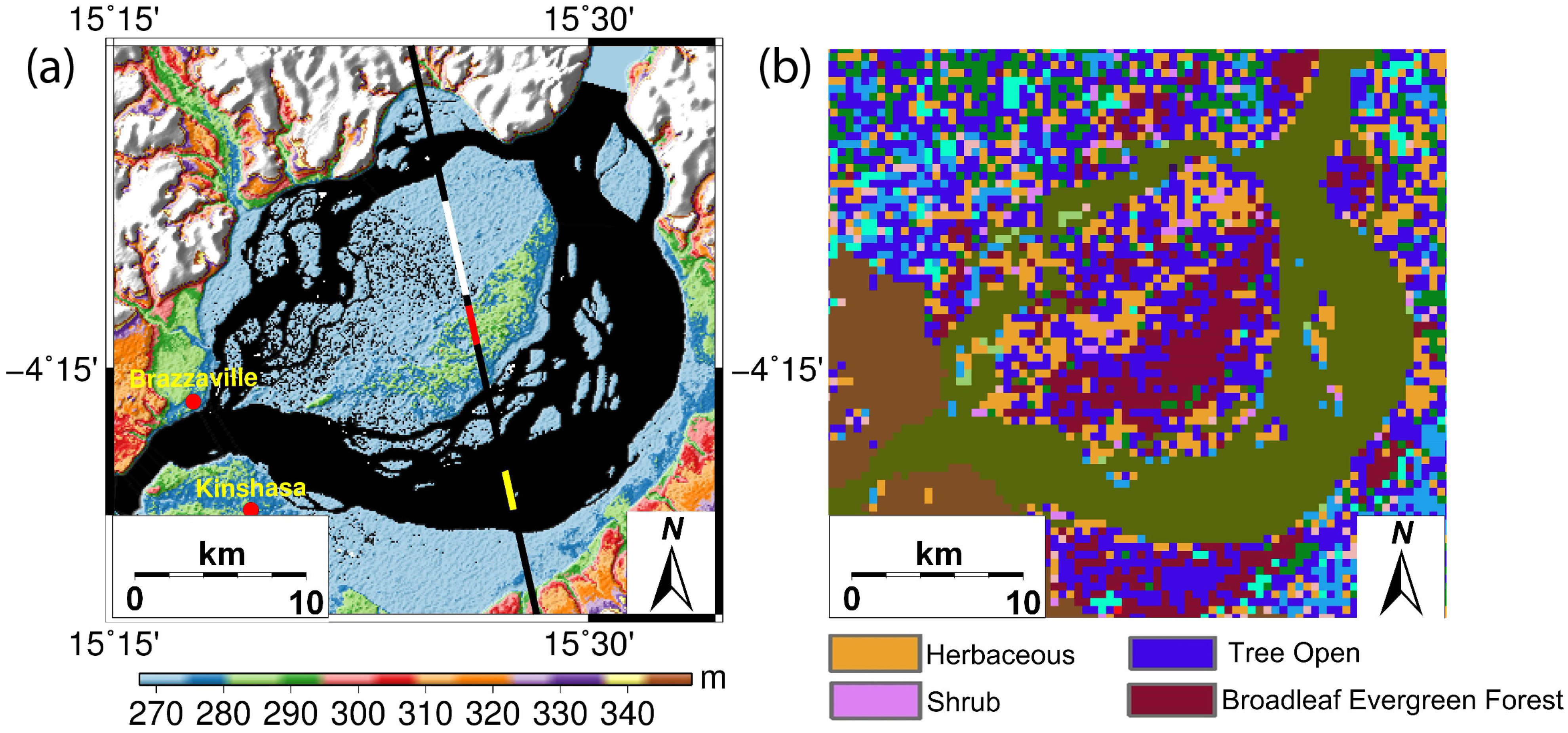
2. Study Area

3. Data Sets
3.1. Envisat Radar Altimetry
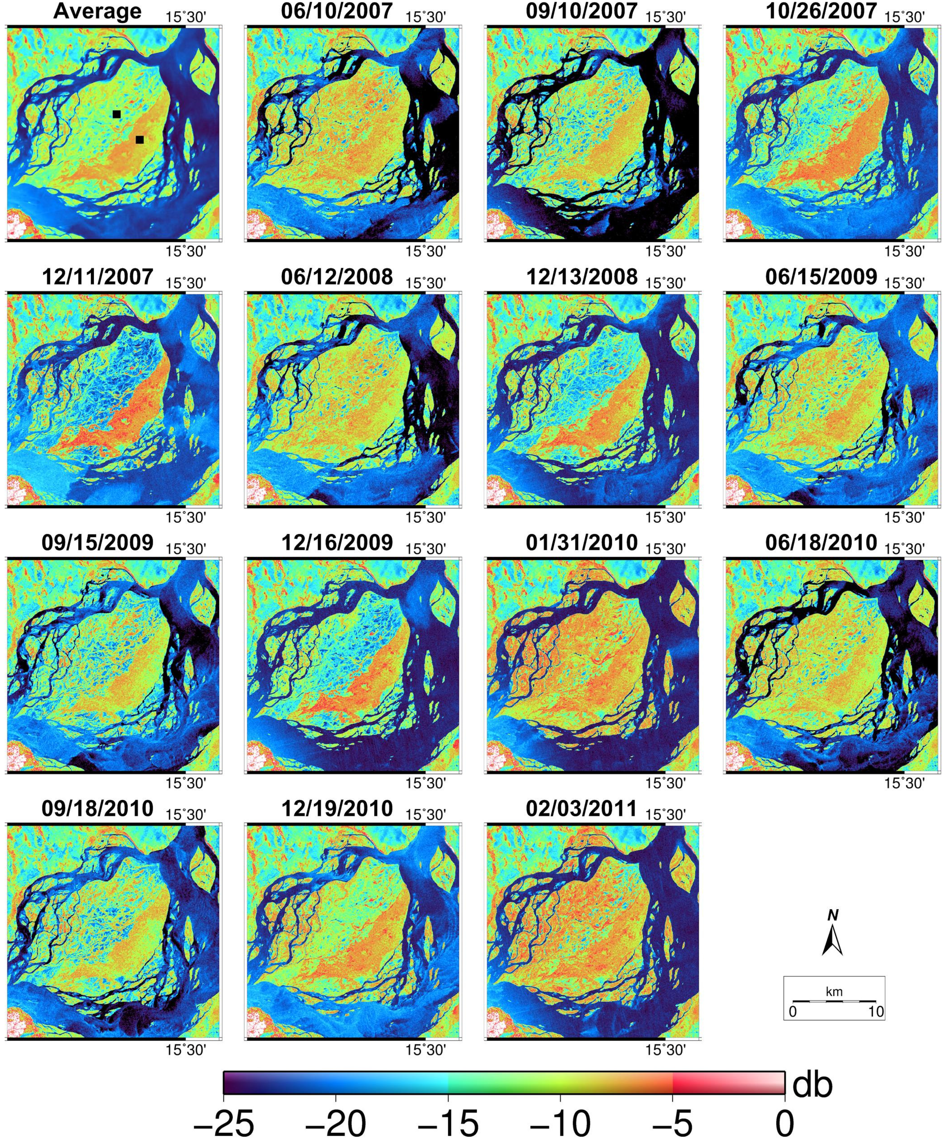
3.2. PALSAR Backscattering Coefficients

| Scene ID | Operation Mode | Date | Path | Frame | Polarization Mode |
|---|---|---|---|---|---|
| ALPSRP073347100 | FBD | 10 June 2007 | 607 | 7100 | HV/HH |
| ALPSRP086767100 | FBD | 10 September 2007 | 607 | 7100 | HV/HH |
| ALPSRP093477100 | FBS | 26 October 2007 | 607 | 7100 | HH |
| ALPSRP100187100 | FBS | 11 December 2007 | 607 | 7100 | HH |
| ALPSRP127027100 | FBD | 12 June 2008 | 607 | 7100 | HV/HH |
| ALPSRP153867100 | FBS | 13 December 2008 | 607 | 7100 | HH |
| ALPSRP180707100 | FBD | 15 June 2009 | 607 | 7100 | HV/HH |
| ALPSRP194127100 | FBD | 15 September 2009 | 607 | 7100 | HV/HH |
| ALPSRP207547100 | FBS | 16 December 2009 | 607 | 7100 | HH |
| ALPSRP214257100 | FBS | 31 January 2010 | 607 | 7100 | HH |
| ALPSRP234387100 | FBD | 18 June 2010 | 607 | 7100 | HV/HH |
| ALPSRP247807100 | FBD | 18 September 2010 | 607 | 7100 | HV/HH |
| ALPSRP261227100 | FBS | 19 December 2010 | 607 | 7100 | HH |
| ALPSRP267937100 | FBS | 3 February 2011 | 607 | 7100 | HH |
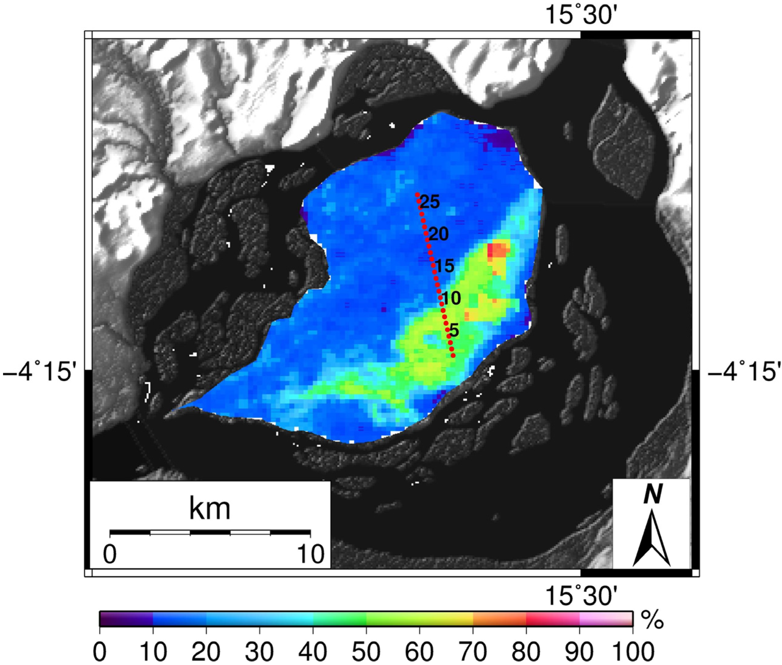
3.3. MODIS VCF
4. Envisat Altimetry and Interferometric SAR Data Processing
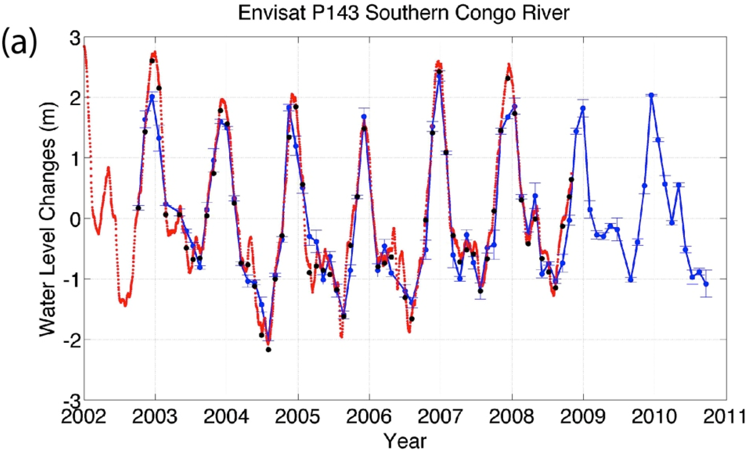
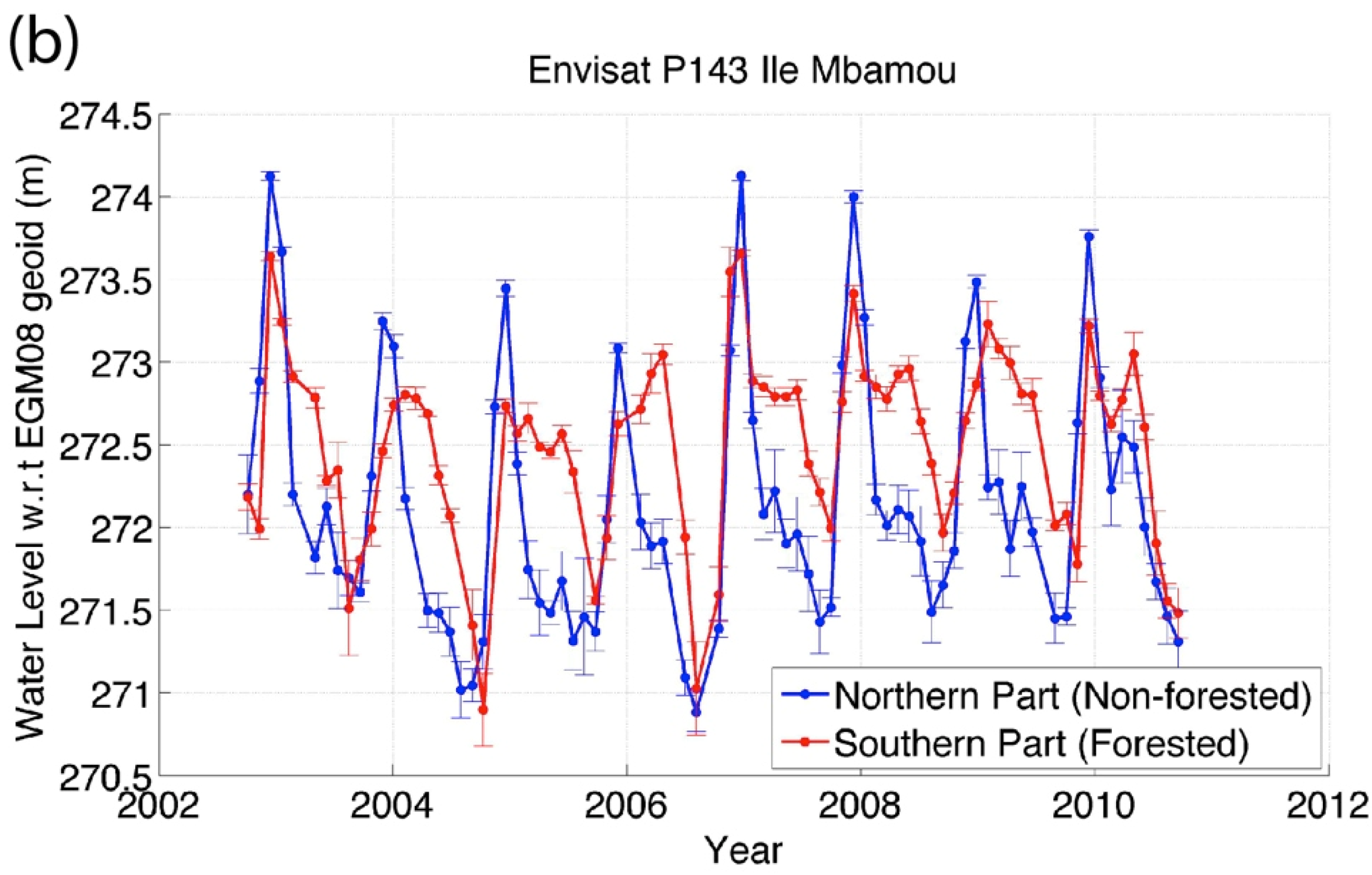
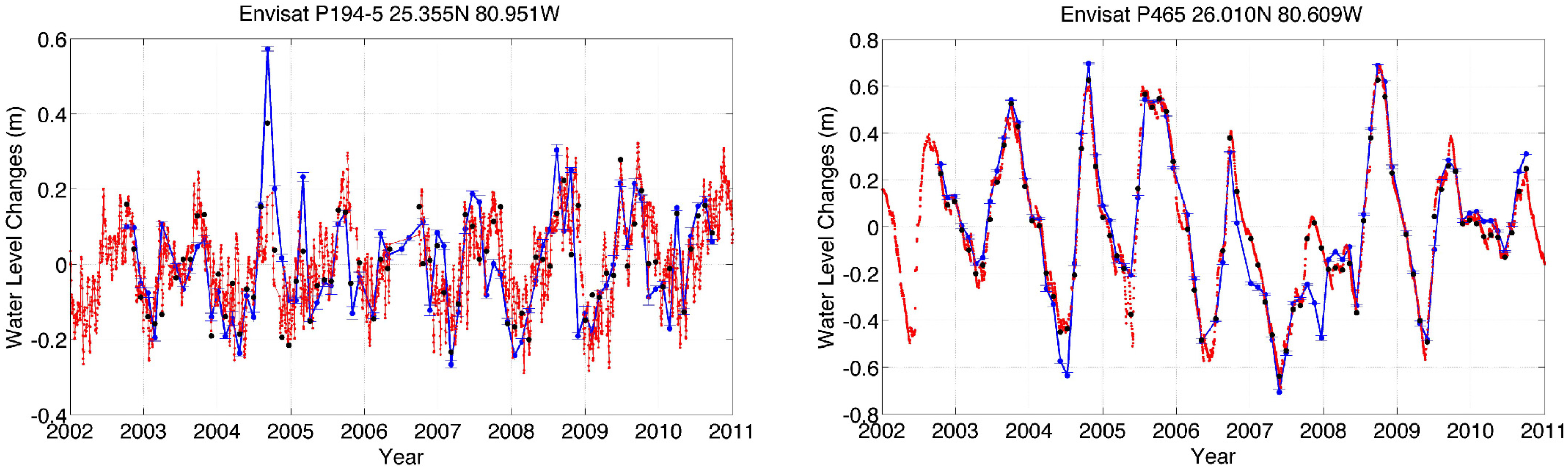
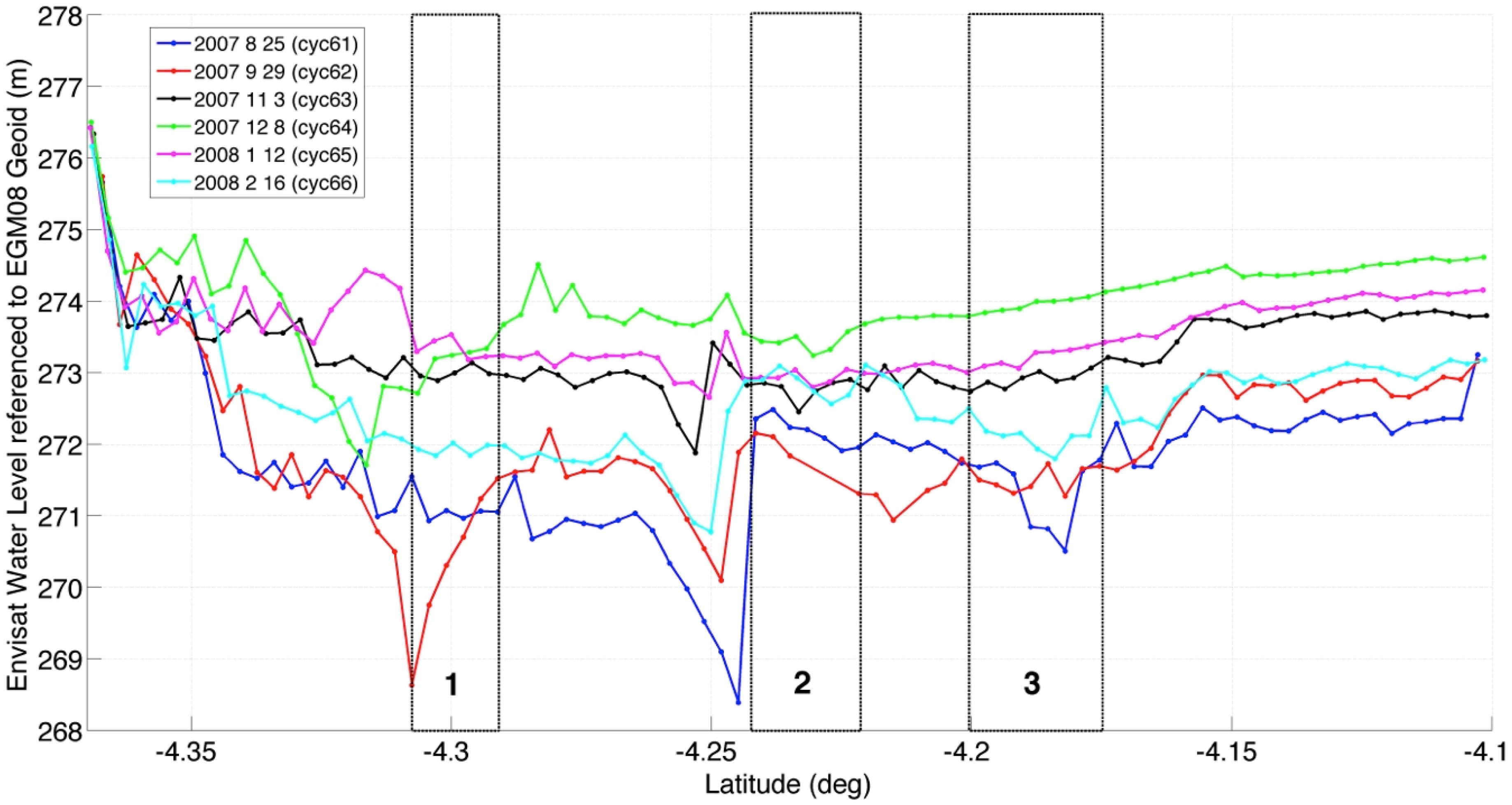
4.1. Water Level Changes from Envisat Altimetry over the Malebo Pool

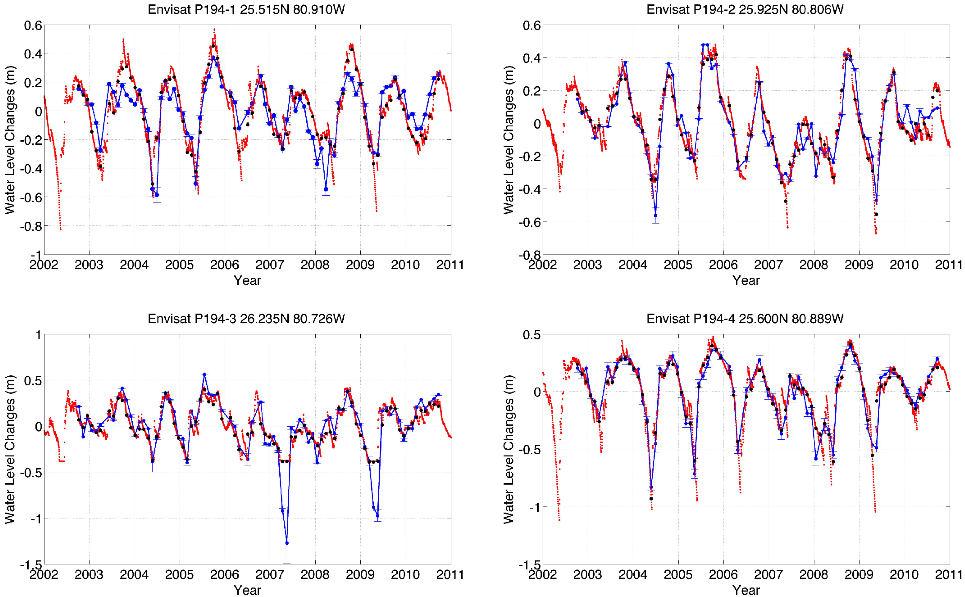
4.2. Comparison of Water Level Changes from Envisat Altimetry over the Everglades and in Situ Data
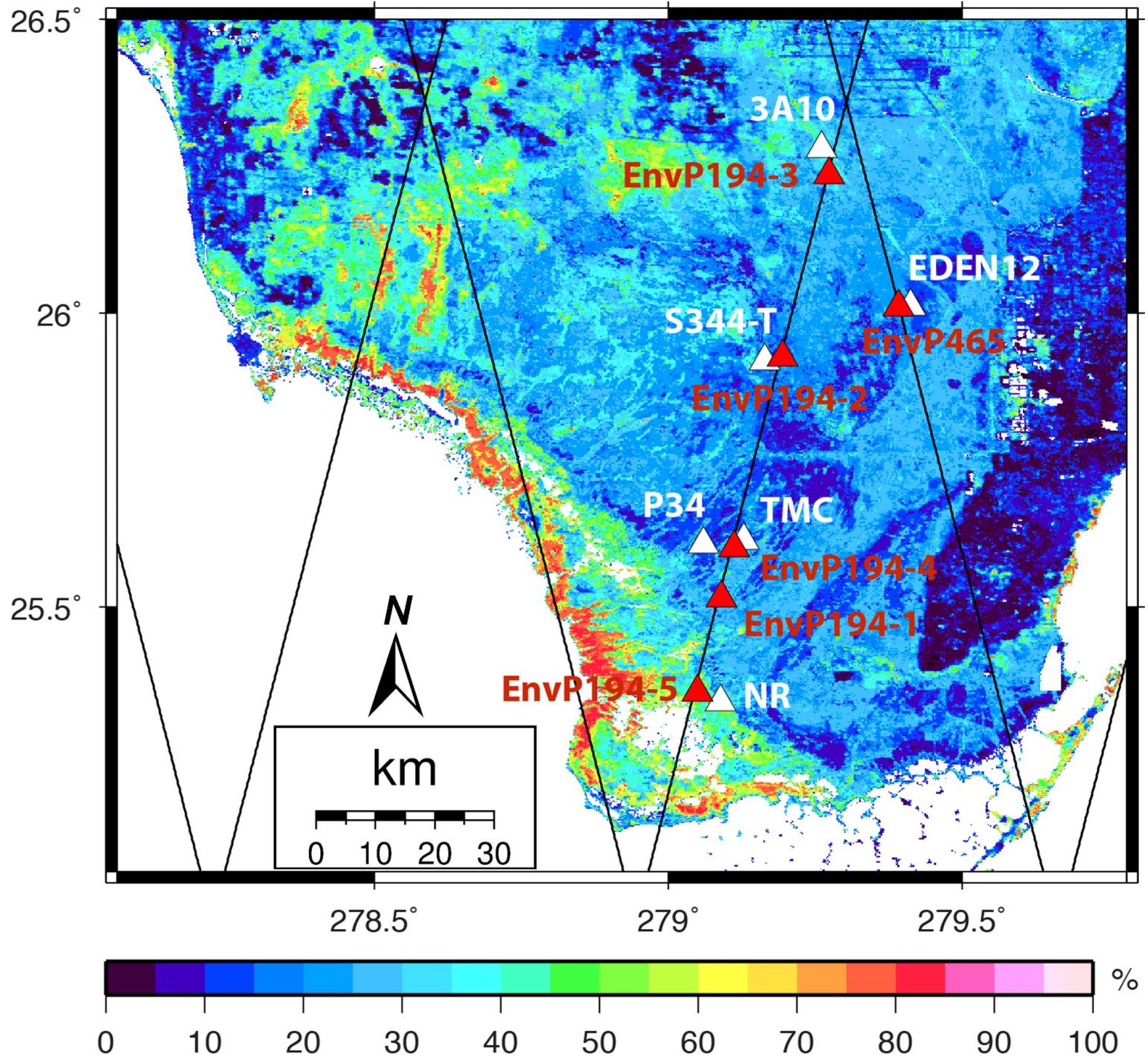

| Altimetry Time Series | In Situ Gauges | Distances between the Altimetry Station and Gauge (km) | RMSE (cm) | Correlation Coefficient | VCF (%) |
|---|---|---|---|---|---|
| EnvP194-1 | P34 | 10.7 | 12.2 | 0.83 | 25 |
| EnvP194-2 | S344-T | 3.2 | 8.6 | 0.92 | 19 |
| EnvP194-3 | 3A10 | 5.1 | 17.1 | 0.87 | 27 |
| EnvP194-4 | TMC | 2.3 | 8.0 | 0.97 | 29 |
| EnvP194-5 | NR | 4.4 | 9.8 | 0.75 | 48 |
| EnvP465 | EDEN12 | 2.1 | 8.6 | 0.96 | 21 |
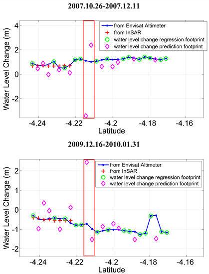
4.3. Water Level Changes over Each Envisat’s High-Rate Nominal Footprint
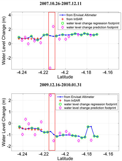
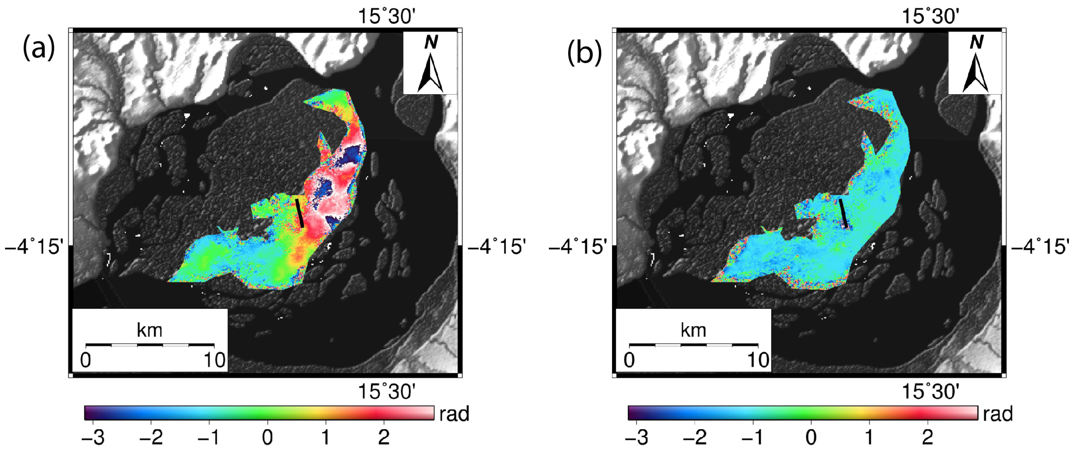
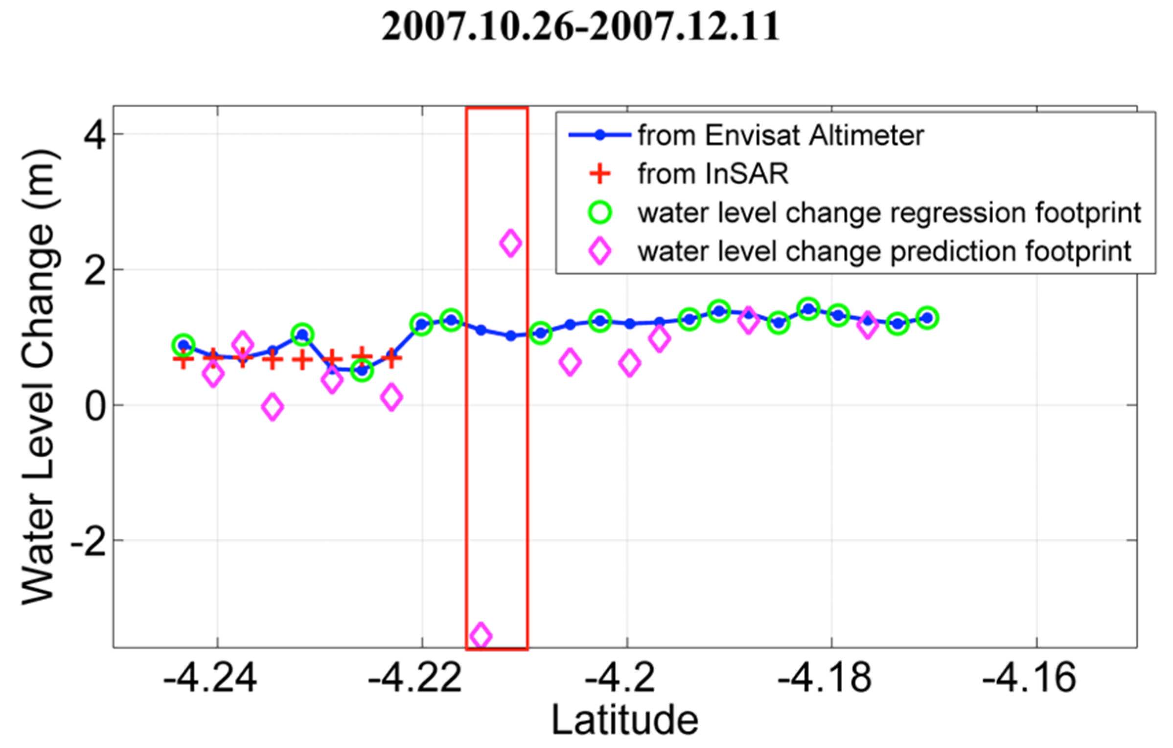
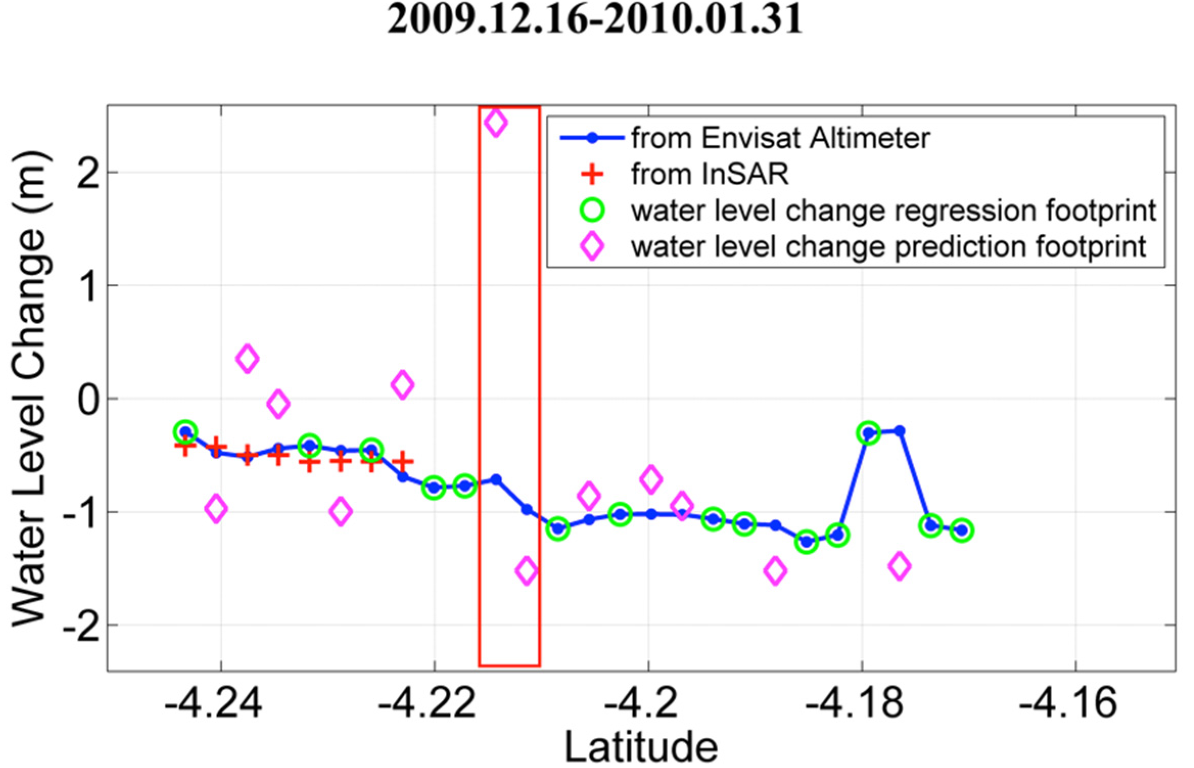
4.4. Water Level Changes from InSAR
| Attribute | Water Increasing Season | Water Decreasing Season |
|---|---|---|
| Perpendicular Baseline | 116 m | 79 m |
| Ambiguity height | 439 m | 645 m |
| Date | 26 October 2007 | 16 December 2009 |
| 11 December 2007 | 31 January 2010 |
5. Estimating Wetland Water Level Changes Based on Changes
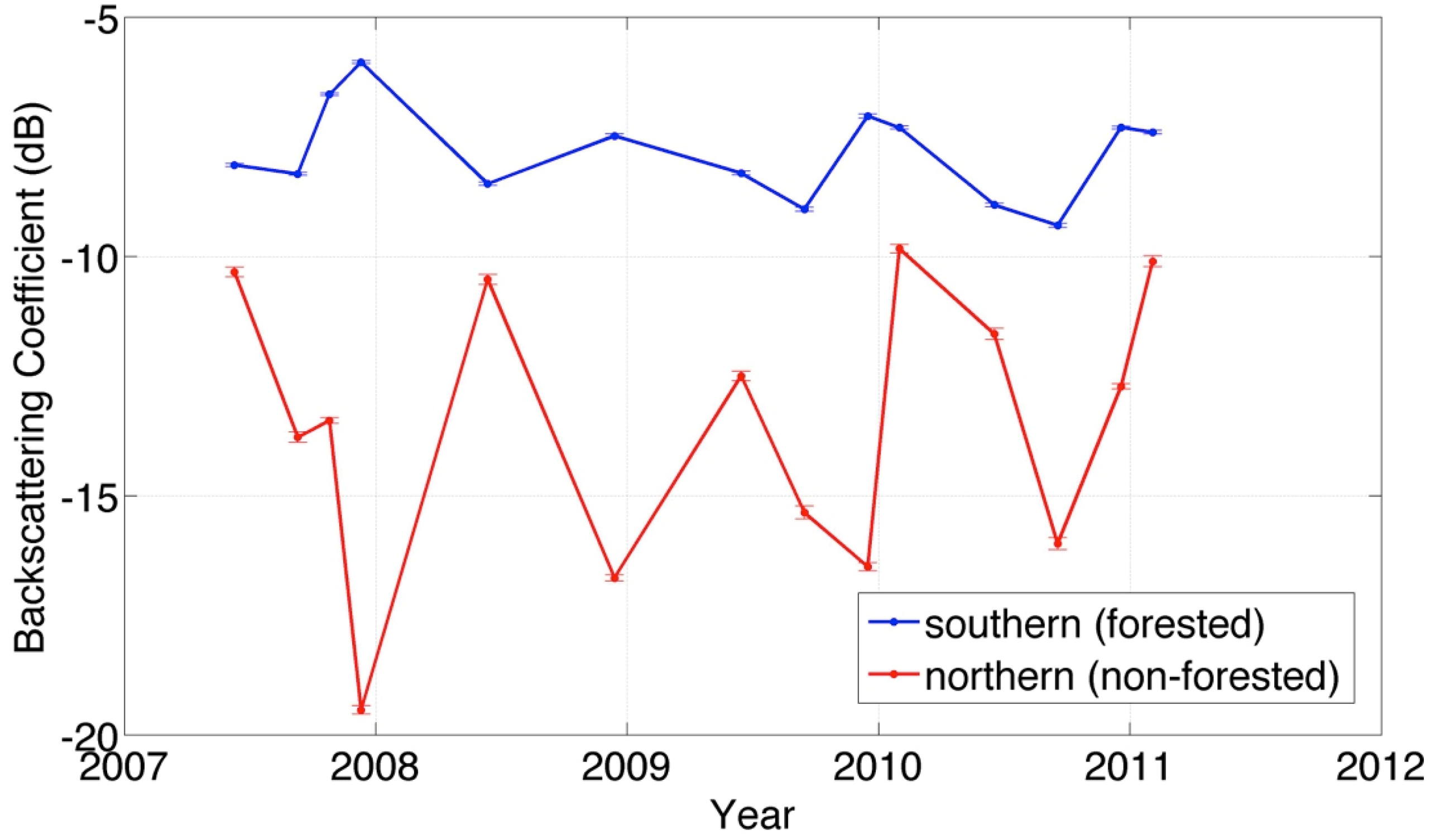
5.1. Temporal Variation of

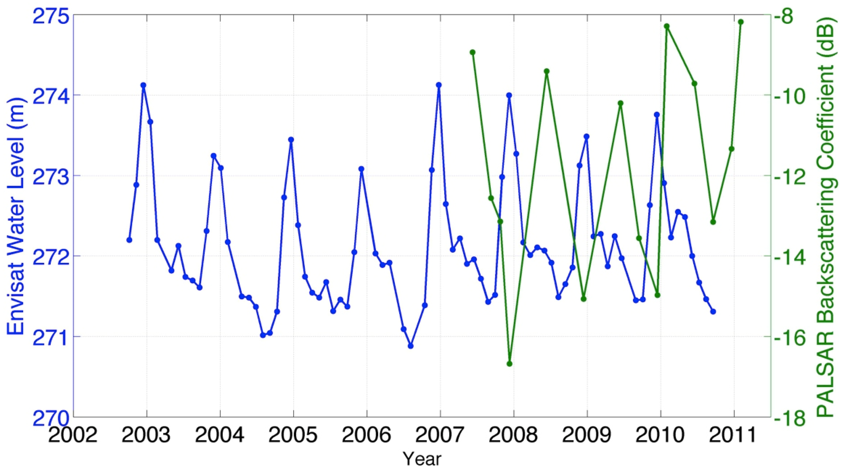
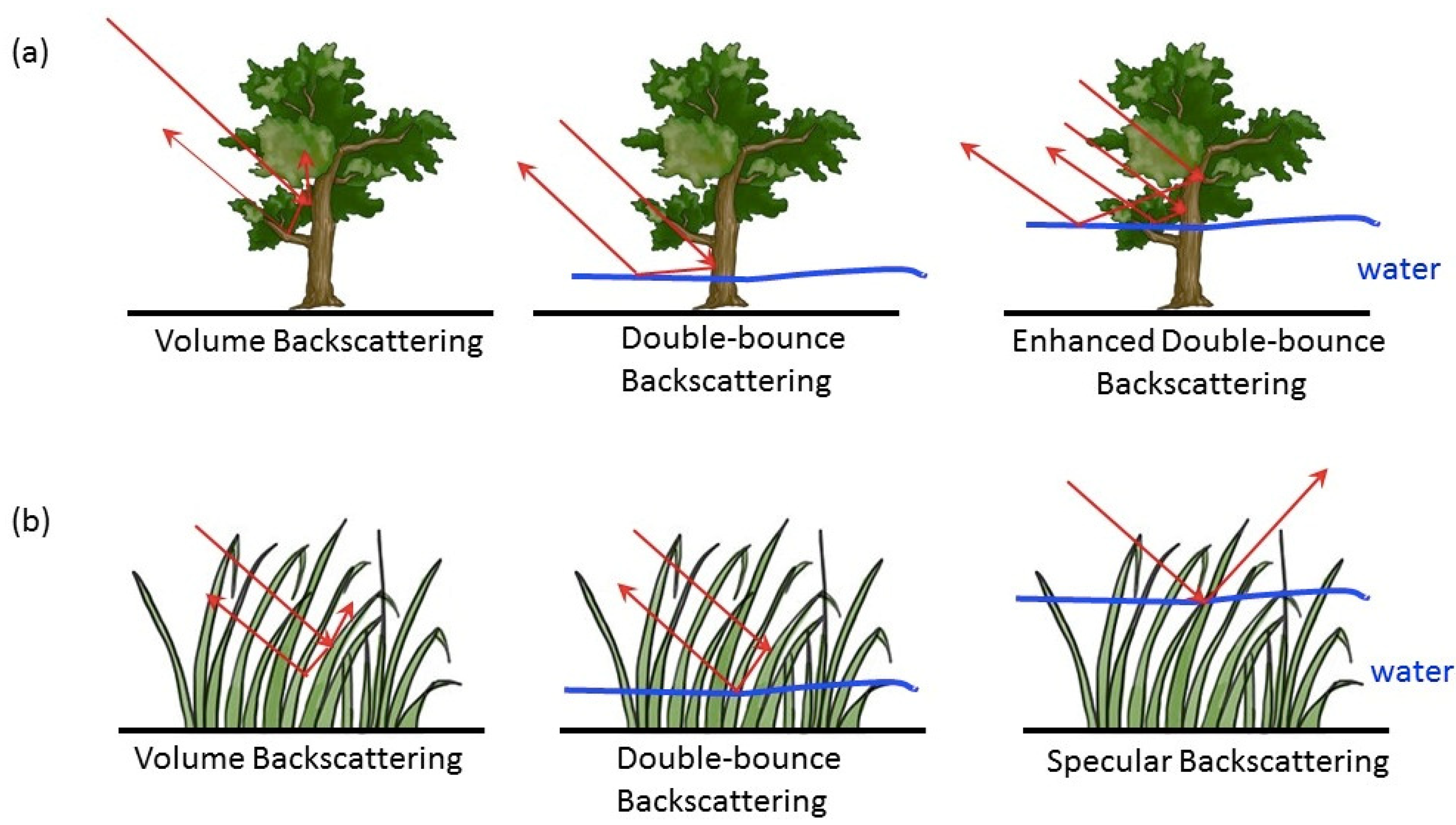
5.2. Effects of Water Level Changes on PALSAR
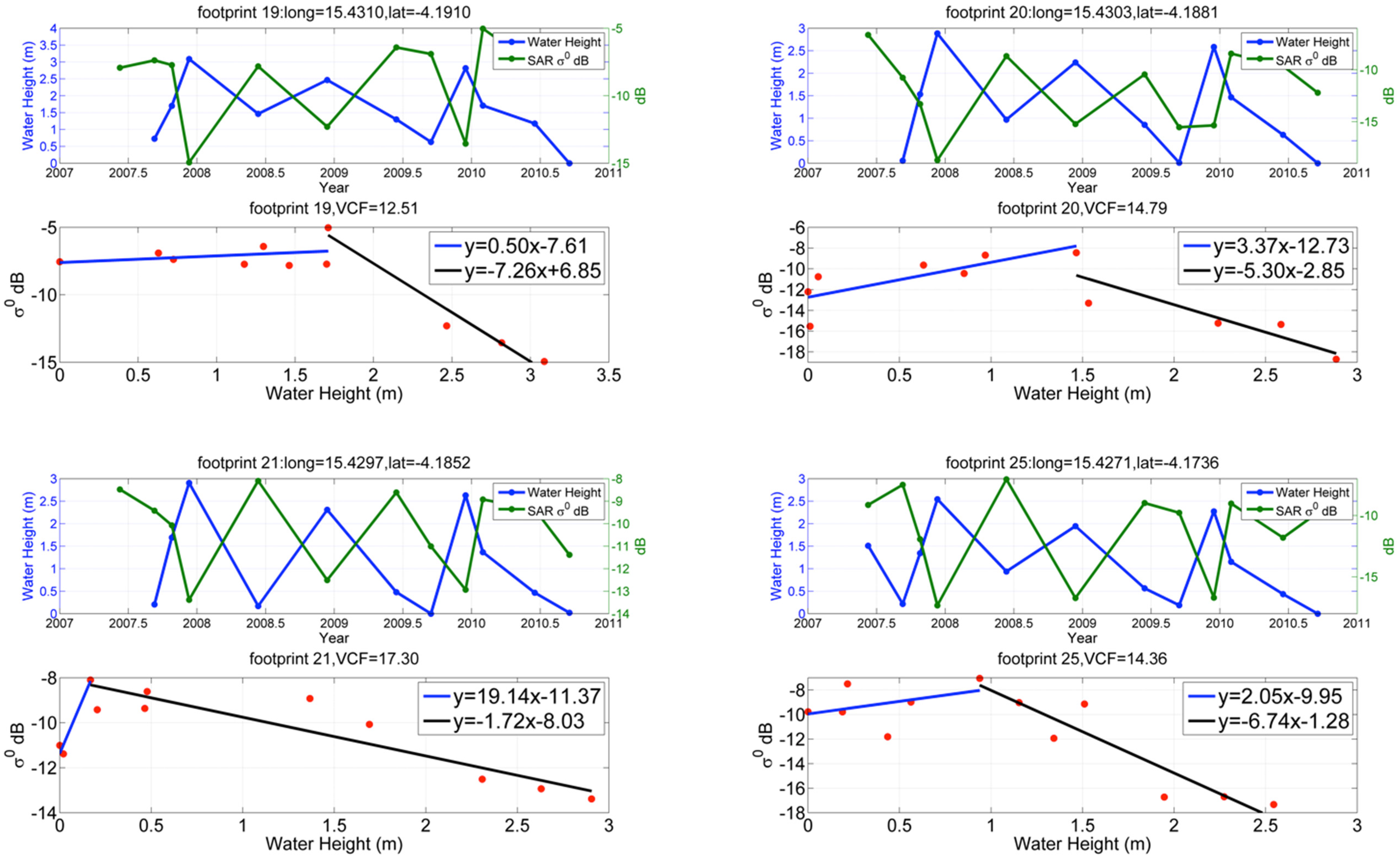
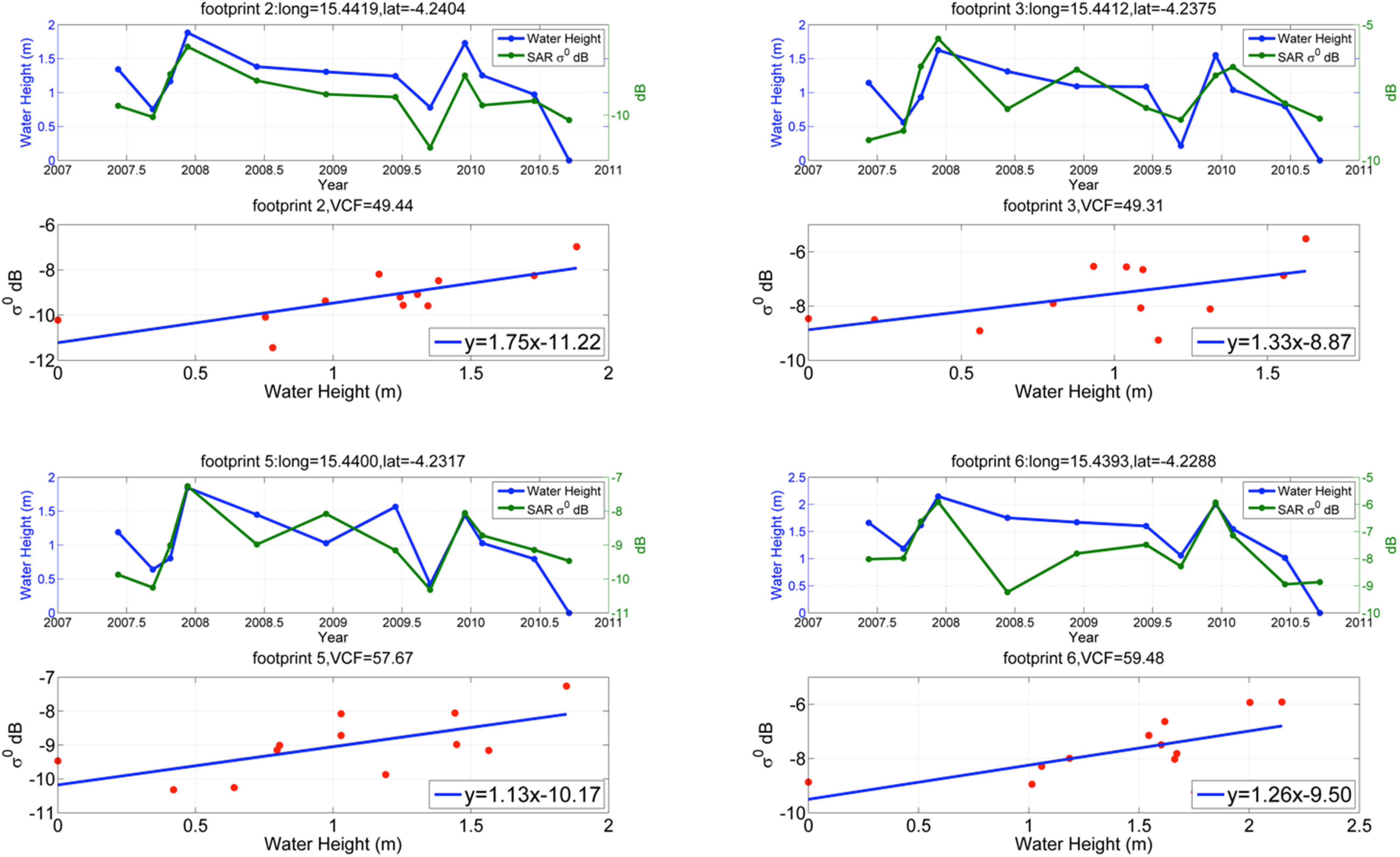
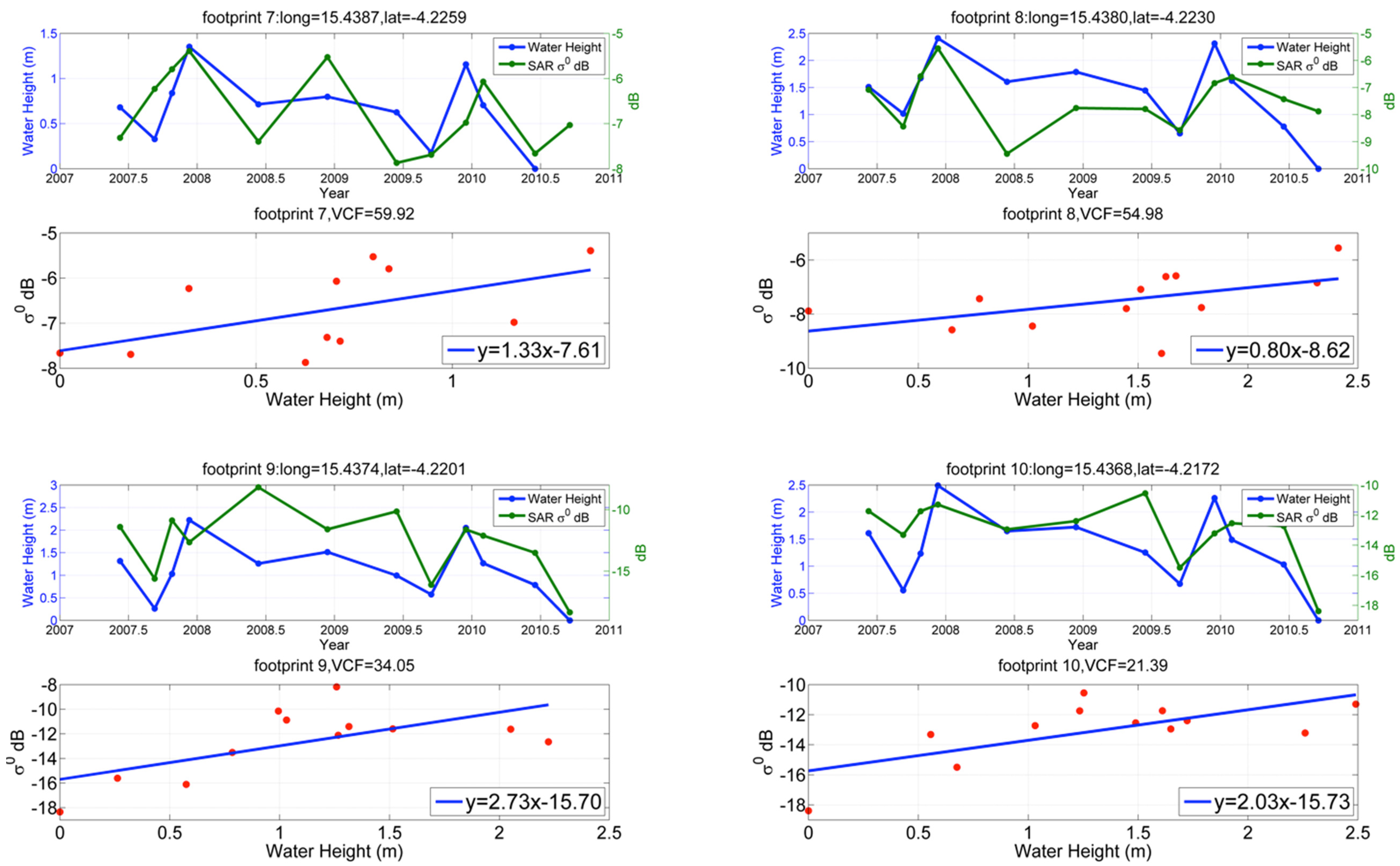
5.2.1. Relationship between Envisat Water Level Changes and PALSAR Changes
5.2.2. Distinguishing Forested and Non-Forested Lands


| Envisat Footprint | Latitude (Degree) | Longitude (Degree) | VCF (%) | Slope | Intercept | R2 |
|---|---|---|---|---|---|---|
| 1 | 15.4425 | −4.2434 | 48.9 | 1.33 | −9.29 | 0.15 |
| 2 | 15.4419 | −4.2404 | 49.4 | 1.75 | −11.2 | 0.56 |
| 3 | 15.4412 | −4.2375 | 49.3 | 1.33 | −8.86 | 0.32 |
| 4 | 15.4406 | −4.2346 | 51.2 | −0.23 | −7.83 | 0.01 |
| 5 | 15.44 | −4.2317 | 57.6 | 1.12 | −10.17 | 0.41 |
| 6 | 15.4393 | −4.2288 | 59.4 | 1.25 | −9.49 | 0.41 |
| 7 | 15.4387 | −4.2259 | 59.9 | 1.32 | −7.6 | 0.31 |
| 8 | 15.438 | −4.223 | 54.9 | 0.8 | −8.62 | 0.27 |
| 9 | 15.4374 | −4.2201 | 34.0 | 2.72 | −15.69 | 0.4 |
| 10 | 15.4368 | −4.2172 | 21.3 | 2.03 | −15.73 | 0.46 |
| Envisat Footprint | Latitude (Degree) | Longitude (Degree) | VCF (%) | Slope 1 | Intercept 1 | R2 | Slope 2 | Intercept 2 | R2 |
|---|---|---|---|---|---|---|---|---|---|
| 11 | 15.4361 | −4.2143 | 19.0 | 2.97 | −16.71 | 0.74 | −10.48 | 6.25 | 0.95 |
| 12 | 15.4355 | −4.2114 | 15.4 | 8.58 | −23.68 | 0.66 | −9.83 | 2.36 | 0.82 |
| 13 | 15.4348 | −4.2085 | 16.7 | 3.51 | −10.49 | 0.64 | −4.90 | −1.35 | 0.96 |
| 14 | 15.4342 | −4.2056 | 15.7 | 2.87 | −8.041 | 0.48 | −2.93 | −2.07 | 0.84 |
| 15 | 15.4335 | −4.2027 | 13.7 | 0.50 | −8.48 | 0.02 | −7.84 | 0.73 | 0.95 |
| 16 | 15.4329 | −4.1998 | 10.1 | 3.35 | −8.67 | 0.22 | −6.27 | −5.56 | 0.84 |
| 17 | 15.4323 | −4.1968 | 11.4 | 4.21 | −13.15 | 0.37 | −8.08 | −1.64 | 0.94 |
| 18 | 15.4316 | −4.1939 | 12.6 | 1.25 | −8.95 | 0.44 | −3.95 | −6.69 | 0.66 |
| 19 | 15.431 | −4.191 | 12.5 | 0.49 | −7.60 | 0.10 | −7.26 | 6.84 | 0.96 |
| 20 | 15.4303 | −4.1881 | 14.7 | 3.36 | −12.73 | 0.61 | −5.29 | −2.85 | 0.78 |
| 21 | 15.4297 | −4.1852 | 17.2 | 19.14 | −11.36 | 0.95 | −1.72 | −8.02 | 0.85 |
| 22 | 15.4291 | −4.1823 | 15.6 | 2.33 | −12.20 | 0.23 | −6.34 | −0.04 | 0.73 |
| 23 | 15.4284 | −4.1794 | 17.4 | 2.79 | −10.91 | 0.81 | −3.41 | −4.20 | 0.50 |
| 24 | 15.4278 | −4.1765 | 15.8 | −2.13 | −7.28 | 0.22 | −17.06 | 29.91 | 0.99 |
| 25 | 15.4271 | −4.1736 | 14.3 | 2.04 | −9.94 | 0.16 | −6.74 | −1.27 | 0.86 |
| 26 | 15.4265 | −4.1707 | 16.1 | 1.98 | −9.70 | 0.34 | −5.22 | −4.63 | 0.60 |
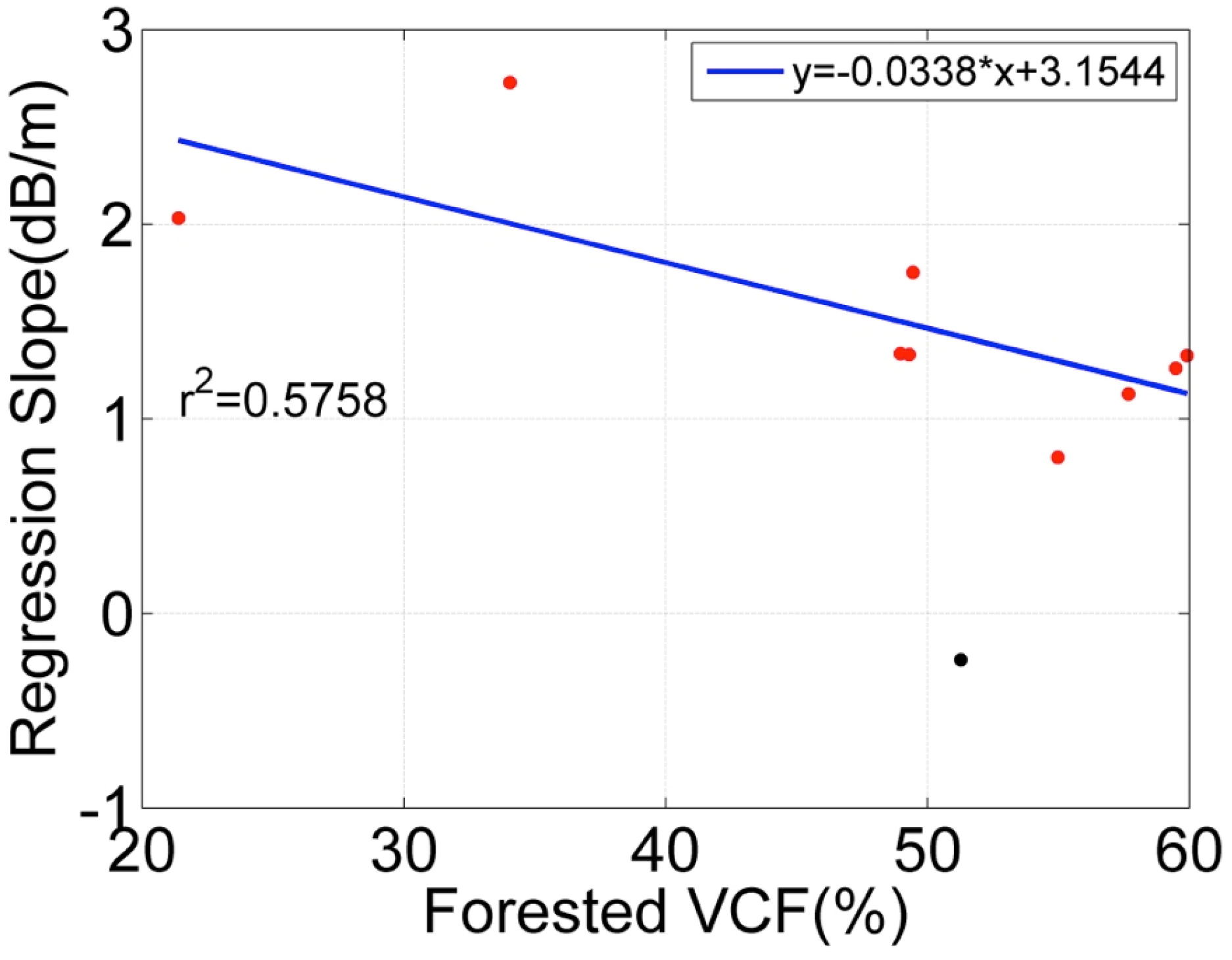
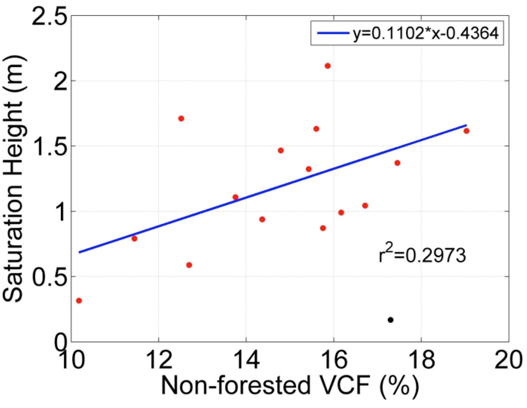
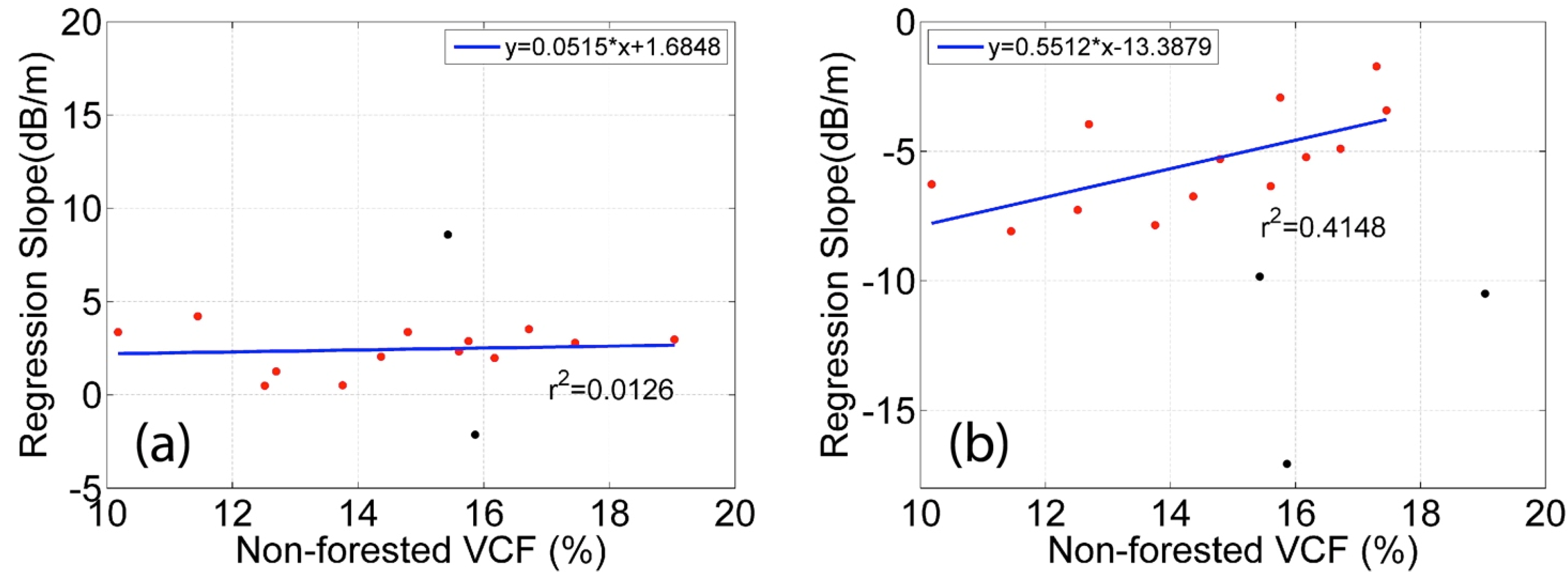
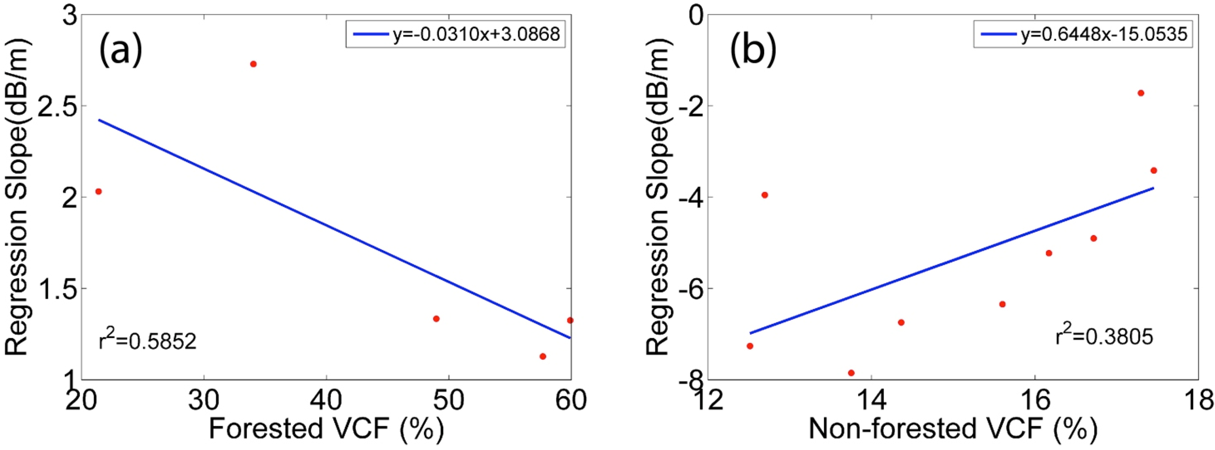
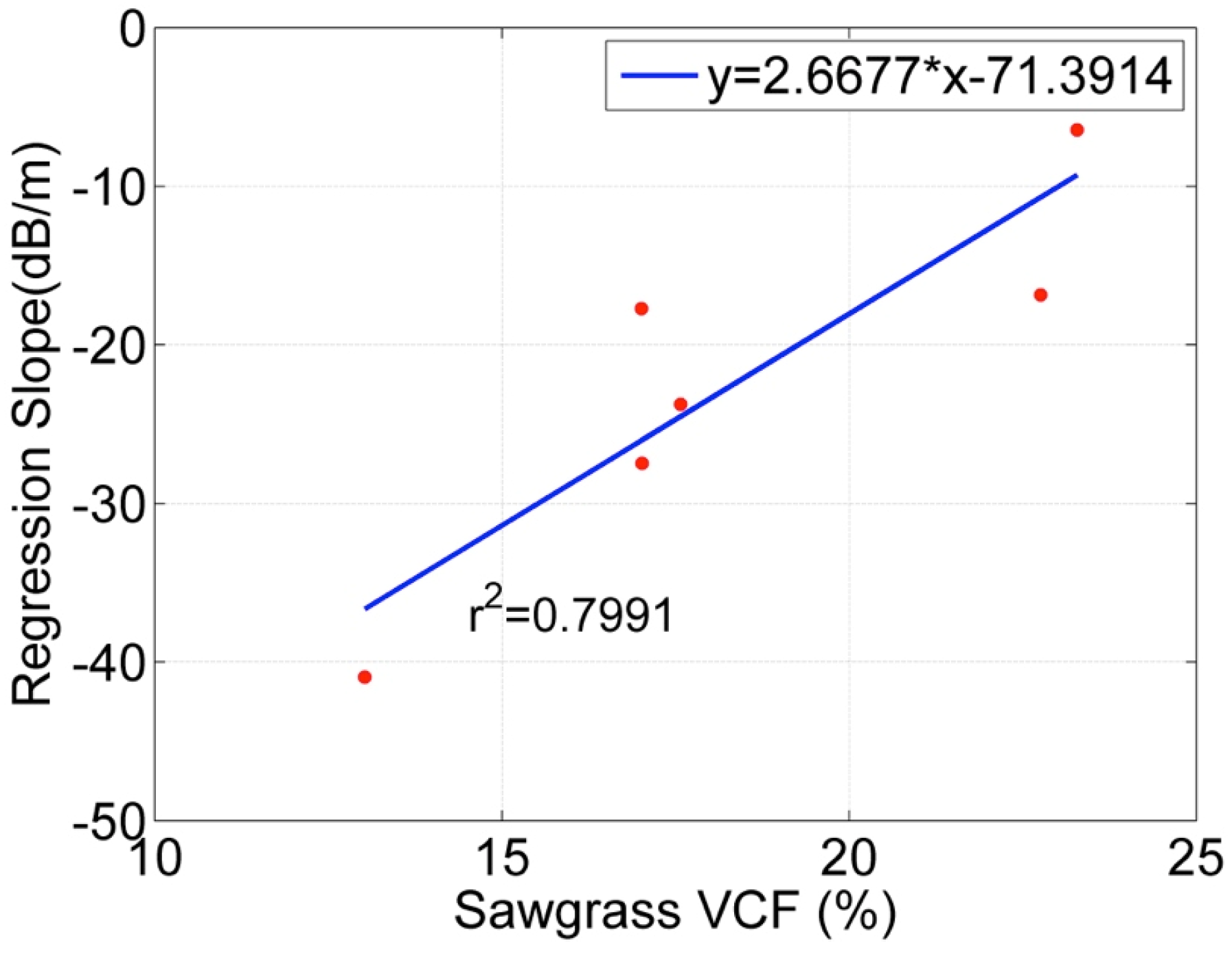
5.2.3. Relationship between the Sensitivity and VCF


5.3. Water Level Changes Estimated from Changes and VCF


| Differences for the Period of 26 October 2007–11 December 2007 (cm) | Differences for the Period of 16 December 2009–31 January 2010 (cm) | |
|---|---|---|
| Forested Land | 25.35 | 49.44 |
| −19.75 | −86.56 | |
| 82.80 | −39.20 | |
| 15.94 | 53.77 | |
| 61.97 | −80.99 | |
| RMSE | 48.95 | 64.69 |
| Non-Forested Land | (452.42) | (−315.31) |
| (−136.88) | (54.33) | |
| 55.48 | −20.67 | |
| 57.98 | −30.43 | |
| 23.87 | −7.70 | |
| 10.06 | 40.32 | |
| 7.56 | 119.36 | |
| RMSE | 37.86 | 58.80 |
6. Application Discussion

7. Conclusions
Acknowledgments
Author Contributions
Conflicts of Interest
References
- Barbier, E.B. Valuing environmental functions: Tropical wetlands. Land Econ. 1994, 70, 155–173. [Google Scholar] [CrossRef]
- Hayashi, M.; van der Kamp, G.; Rudolph, D.L. Water and solute transfer between a prairie wetland and adjacent uplands, 2. Chloride cycle. J Hydrol. 1998, 207, 56–67. [Google Scholar] [CrossRef]
- Neue, H.U.; Gaunt, J.L.; Wang, Z.P.; Becker-Heidmann, P.; Quijano, C. Carbon in tropical wetlands. Geoderma 1997, 79, 163–185. [Google Scholar] [CrossRef]
- Mitsch, W.J.; Gosselink, J.G. Wetlands, 4th ed.; John Wiley and Sons: New York, NY, USA, 2007. [Google Scholar]
- Jung, H.C.; Hamski, J.; Durand, M.; Alsdorf, D.; Hossain, F.; Lee, H.; Azad Hossain, A.K.M.; Hasan, K.; Khan, A.S.; Zeaul Hoque, A.K.M. Characterization of complex fluvial systems using remote sensing of spatial and temporal water level variations in the Amazon, Congo, and Brahmaputra rivers. Earth Surf. Process. Landf. 2010, 35, 294–304. [Google Scholar] [CrossRef]
- Beighley, R.E.; Ray, R.L.; He, Y.; Lee, H.; Schaller, L.; Andreadis, K.M.; Durand, M.; Alsdorf, D.E.; Shum, C.K. Comparing satellite derived precipitation datasets using the Hillslope River Routing (HRR) model in the Congo River Basin. Hydrol. Process. 2011, 25, 3216–3229. [Google Scholar] [CrossRef]
- Lee, H.; Beighley, R.E.; Alsdorf, D.; Jung, H.C.; Shum, C.K.; Duan, J.; Guo, J.; Yamazaki, D.; Andreadis, K. Characterization of terrestrial water dynamics in the Congo Basin using GRACE and satellite radar altimetry. Remote Sens. Environ. 2011, 115, 3530–3538. [Google Scholar] [CrossRef]
- Alsdorf, D.E.; Smith, L.C.; Melack, J.M. Amazon floodplain water level changes measured with interferometric SIR-C radar. IEEE Trans. Geosci. Remote Sens. 2001, 39, 423–431. [Google Scholar] [CrossRef]
- Alsdorf, D.; Bates, P.; Melack, J.; Wilson, M.; Dunne, T. Spatial and temporal complexity of the Amazon flood measured from space. Geophys. Res. Lett. 2007, 34, 1–5. [Google Scholar]
- Wdowinski, S.; Kim, S.W.; Amelung, F.; Dixon, T.H.; Miralles-Wilhelm, F.; Sonenshein, R. Space-based detection of wetlands’ surface water level changes from L-band SAR interferometry. Remote Sens. Environ. 2008, 112, 681–696. [Google Scholar] [CrossRef]
- Lu, Z.; Kwoun, O.I. Radarsat-1 and ERS InSAR analysis over southeastern coastal Louisiana: Implications for mapping water-level changes beneath swamp forests. IEEE Trans. Geosci. Remote Sens. 2008, 46, 2167–2184. [Google Scholar] [CrossRef]
- Chul Jung, H.; Alsdorf, D. Repeat-pass multi-temporal interferometric SAR coherence variations with Amazon floodplain and lake habitats. Int. J. Remote Sens. 2010, 31, 881–901. [Google Scholar] [CrossRef]
- Kim, S.W.; Hong, S.H.; Won, J.S. An application of L-band synthetic aperture radar to tide height measurement. IEEE Trans. Geosci. Remote Sens. 2005, 43, 1472–1478. [Google Scholar] [CrossRef]
- Kim, J.W.; Lu, Z.; Lee, H.; Shum, C.K.; Swarzenski, C.M.; Doyle, T.W.; Baek, S.H. Integrated analysis of PALSAR/Radarsat-1 InSAR and ENVISAT altimeter data for mapping of absolute water level changes in Louisiana wetlands. Remote Sens. Environ. 2009, 113, 2356–2365. [Google Scholar] [CrossRef]
- Hess, L.L.; Melack, J.M.; Novo, E.M.L.M.; Barbosa, C.C.F.; Gastil, M. Dual-season mapping of wetland inundation and vegetation for the central Amazon basin. Remote Sens. Environ. 2003, 87, 404–428. [Google Scholar] [CrossRef]
- Martinez, J.M.; Le Toan, T. Mapping of flood dynamics and spatial distribution of vegetation in the Amazon floodplain using multitemporal SAR data. Remote Sens. Environ. 2007, 108, 209–223. [Google Scholar] [CrossRef]
- Kasischke, E.S.; Smith, K.B.; Bourgeau-Chavez, L.L.; Romanowicz, E.A.; Brunzell, S.; Richardson, C.J. Effects of seasonal hydrologic patterns in south Florida wetlands on radar backscatter measured from ERS-2 SAR imagery. Remote Sens. Environ. 2003, 88, 423–441. [Google Scholar] [CrossRef]
- Grings, F.M.; Ferrazzoli, P.; Jacobo-Berlles, J.C.; Karszenbaum, H.; Tiffenberg, J.; Pratolongo, P.; Kandus, P. Monitoring flood condition in marshes using EM models and Envisat ASAR observations. IEEE Trans. Geosci. Remote Sens. 2006, 44, 936–941. [Google Scholar] [CrossRef]
- Grings, F.M.; Ferrazzoli, P.; Karszenbaum, H.; Salvia, M.; Kandus, P.; Jacobo-Berlles, J.C.; Perna, P. Model investigation about the potential of C band SAR in herbaceous wetlands flood monitoring. Int. J. Remote Sens. 2008, 29, 5361–5372. [Google Scholar] [CrossRef]
- Trung, V.N.; Choi, J.H.; Won, J.S. A land cover variation model of water level for the floodplain of Tonle Sap, Cambodia, derived from ALOS PALSAR and MODIS data. IEEE J. Sel. Top Appl. Earth Obs. Remote Sens. 2013, 6, 2238–2253. [Google Scholar] [CrossRef]
- Kim, J.-W.; Lu, Z.; Jones, J.W.; Shum, C.K.; Lee, H.; Jia, Y. Monitoring everglades freshwater marsh water level using L-band synthetic aperture radar backscatter. Remote Sens. Environ. 2014, 150, 66–81. [Google Scholar] [CrossRef]
- Lee, H.; Shum, C.K.; Yi, Y.; Ibaraki, M.; Kim, J.-W.; Braun, A.; Kuo, C.-Y.; Lu, Z. Louisiana wetland water level monitoring using retracked TOPEX/POSEIDON altimetry. Mar. Geod. 2009, 32, 284–302. [Google Scholar] [CrossRef]
- Birkett, C.M.; Mertes, L.A.K.; Dunne, T.; Costa, M.H.; Jasinski, M.J. Surface water dynamics in the Amazon Basin: Application of satellite radar altimetry. J. Geophys. Res.: Atmos. 2002, 107, LBA 26-1–LBA 26-21. [Google Scholar] [CrossRef]
- Lee, H.; Jung, H.C.; Yuan, T.; Beighley, R.E.; Duan, J. Controls of terrestrial water storage changes over the central Congo Basin determined by integrating PALSAR ScanSAR, Envisat altimetry, and GRACE data. In Remote Sensing of the Terrestrial Water Cycle; John Wiley & Sons, Inc: Hoboken, NJ, USA, 2014; pp. 115–129. [Google Scholar]
- Hansen, M.C.; DeFries, R.S.; Townshend, J.R.G.; Carroll, M.; Dimiceli, C.; Sohlberg, R.A. Global percent tree cover at a spatial resolution of 500 meters: First results of the MODIS vegetation continuous fields algorithm. Earth Interact. 2003, 7, 1–15. [Google Scholar] [CrossRef]
- DiMiceli, C.M.; Carroll, M.L.; Sohlberg, R.A.; Huang, C.; Hansen, M.C.; Townshend, J.R.G. Annual Global Automated MODIS Vegetation Continuous Fields (MOD44B) at 250 m Spatial Resolution for Data Years Beginning Day 65, 2000–2010; Collection 5 Percent Tree Cover; University of Maryland: College Park, MD, USA, 2010. [Google Scholar]
- Bailey, R.G.; Banister, K.E. The Zaïre River system. In The Ecology of River Systems; Davies, B.R., Walker, K.F., Eds.; Springer Netherlands: Dordrecht, The Netherlands, 1986; Volume 60, pp. 201–224. [Google Scholar]
- Thieme, M.L.; Abell, R.; Burgess, N.; Lehner, B.; Dinerstein, E.; Olson, D. Freshwater Ecoregions of Africa and Madagascar: A Conservation Assessment; Island Press: Washington, DC, USA, 2005. [Google Scholar]
- Baugh, C.A.; Bates, P.D.; Schumann, G.; Trigg, M.A. SRTM vegetation removal and hydrodynamic modeling accuracy. Water Resour. Res. 2013, 49, 5276–5289. [Google Scholar] [CrossRef]
- Brown, C.G.; Sarabandi, K.; Pierce, L.E. Model-based estimation of forest canopy height in red and Austrian pine stands using shuttle radar topography mission and ancillary data: A proof-of-concept study. IEEE Trans. Geosci. Remote Sens. 2010, 48, 1105–1118. [Google Scholar] [CrossRef]
- Tateishi, R.; Uriyangqai, B.; Al-Bilbisi, H.; Ghar, M.A.; Tsend-Ayush, J.; Kobayashi, T.; Kasimu, A.; Hoan, N.T.; Shalaby, A.; Alsaaideh, B.; Enkhzaya, T.; Gegentana; Sato, H.P. Production of global land cover data—GLCNMO. Int. J. Digit. Earth. 2010, 4, 22–49. [Google Scholar] [CrossRef]
- Sita, P. Etude préliminaire de la végétation de l’île M'Bamou. Available online: http://horizon.documentation.ird.fr/exl-doc/pleins_textes/divers12-05/12250.pdf (accessed on 20 December 2014).
- Wingham, D.J.; Rapley, C.G.; Griffiths, H. New techniques in satellite altimeter tracking systems. In Proceedings of 1986 International Geoscience and Remote Sensing Symposium (IGARSS’86) on Remote Sensing: Today’s Solutions for Tomorrow’s Information Needs; ESA Publication Division: Noordwijk, The Netherlands, 1986; Volume 3. [Google Scholar]
- Rosenqvist, A.; Shimada, M.; Ito, N.; Watanabe, M. ALOS PALSAR: A pathfinder mission for global-scale monitoring of the environment. IEEE Trans. Geosci. Remote Sens. 2007, 45, 3307–3316. [Google Scholar] [CrossRef]
- Pope, K.O.; Rejmankova, E.; Paris, J.F.; Woodruff, R. Detecting seasonal flooding cycles in marshes of the Yucatan Peninsula with SIR-C polarimetric radar imagery. Remote Sens. Environ. 1997, 59, 157–166. [Google Scholar] [CrossRef]
- Grings, F.; Salvia, M.; Karszenbaum, H.; Ferrazzoli, P.; Kandus, P.; Perna, P. Exploring the capacity of radar remote sensing to estimate wetland marshes water storage. J. Environ. Manage. 2009, 90, 2189–2198. [Google Scholar] [CrossRef] [PubMed]
- Shimada, M.; Isoguchi, O.; Tadono, T.; Isono, K. PALSAR radiometric and geometric calibration. IEEE Trans. Geosci. Remote Sens. 2009, 47, 3915–3932. [Google Scholar] [CrossRef]
- Werner, C.; Wegmüller, U.; Strozzi, T.; Wiesmann, A. Gamma SAR and interferometric processing software. In Proc of ERS-Envisat Symp; Citeseer: Gothenburg, Sweden, 2000; Volumer 461. [Google Scholar]
- NASA Shuttle Radar Topography Mission. Available online: https://lpdaac.usgs.gov/products/measures_products_table/srtmgl1 (accessed on 15 February 2015).
- Lee, H.; Shum, C.K.; Yi, Y.; Braun, A.; Kuo, C.-Y.Y. Laurentia crustal motion observed using TOPEX/POSEIDON radar altimetry over land. J. Geodyn. 2008, 46, 182–193. [Google Scholar] [CrossRef]
- Kruizinga, G.J. Dual-Satellite Altimeter Crossover Measurements for Precise Orbit Determination. Ph.D. Dissertation, University of Texas, Austin, TX, USA, 1997. [Google Scholar]
- Wegmuller, U. Automated terrain corrected SAR geocoding. In Proceedings of IEEE 1999 International Geoscience and Remote Sensing Symposium, Hamburg, Germany, 28 June–2 July 1999; Volume 3, pp. 1712–1714.
- Nelson, M.D.; McRoberts, R.E.; Hansen, M.C. Forest land area estimates from Vegetation Continuous Fields. In Proceedings of Proceedings of the Tenth Biennial Forest Service Remote Sensing Applications Conference—Remote Sensing for Field Users, Salt Lake City, UT, USA, 5–9 April 2004; pp. 5–9.
- Schmitt, C.B.; Burgess, N.D.; Coad, L.; Belokurov, A.; Besançon, C.; Boisrobert, L.; Campbell, A.; Fish, L.; Gliddon, D.; Humphries, K. Global analysis of the protection status of the world’s forests. Biol. Conserv. 2009, 142, 2122–2130. [Google Scholar] [CrossRef]
- Hansen, M.C.; Roy, D.P.; Lindquist, E.; Adusei, B.; Justice, C.O.; Altstatt, A. A method for integrating MODIS and Landsat data for systematic monitoring of forest cover and change in the Congo Basin. Remote Sens. Environ. 2008, 112, 2495–2513. [Google Scholar] [CrossRef]
- Costa, M.P.F.; Niemann, O.; Novo, E.; Ahern, F. Biophysical properties and mapping of aquatic vegetation during the hydrological cycle of the Amazon floodplain using JERS-1 and Radarsat. Int. J. Remote Sens. 2002, 23, 1401–1426. [Google Scholar] [CrossRef]
- Le Toan, T.; Ribbes, F.; Wang, L.-F.; Floury, N.; Ding, K.-H.; Kong, J.A.; Fujita, M.; Kurosu, T. Rice crop mapping and monitoring using ERS-1 data based on experiment and modeling results. IEEE Trans. Geosci. Remote Sens. 1997, 35, 41–56. [Google Scholar] [CrossRef]
- Kwoun, O.; Lu, Z. Multi-temporal RADARSAT-1 and ERS backscattering signatures of coastal wetlands in southeastern Louisiana. Photogramm. Eng. Remote Sens. 2009, 75, 607–617. [Google Scholar] [CrossRef]
- Alsdorf, D.E.; Rodríguez, E.; Lettenmaier, D.P. Measuring surface water from space. Rev. Geophys. 2007. [Google Scholar] [CrossRef]
- Wilson, M.D.; Bates, P.; Alsdorf, D.; Forsberg, B.; Horritt, M.; Melack, J.; Frappart, F.; Famiglietti, J. Modeling large-scale inundation of Amazonian seasonally flooded wetlands. Geophys. Res. Lett. 2007, 34, 4–9. [Google Scholar]
- Jung, H.C.; Jasinski, M.; Kim, J.W.; Shum, C.K.; Bates, P.; Neal, J.; Lee, H.; Alsdorf, D. Calibration of two-dimensional floodplain modeling in the central Atchafalaya Basin Floodway System using SAR interferometry. Water Resour. Res. 2012, 48, 1–13. [Google Scholar] [CrossRef]
© 2015 by the authors; licensee MDPI, Basel, Switzerland. This article is an open access article distributed under the terms and conditions of the Creative Commons Attribution license (http://creativecommons.org/licenses/by/4.0/).
Share and Cite
Yuan, T.; Lee, H.; Jung, H.C. Toward Estimating Wetland Water Level Changes Based on Hydrological Sensitivity Analysis of PALSAR Backscattering Coefficients over Different Vegetation Fields. Remote Sens. 2015, 7, 3153-3183. https://doi.org/10.3390/rs70303153
Yuan T, Lee H, Jung HC. Toward Estimating Wetland Water Level Changes Based on Hydrological Sensitivity Analysis of PALSAR Backscattering Coefficients over Different Vegetation Fields. Remote Sensing. 2015; 7(3):3153-3183. https://doi.org/10.3390/rs70303153
Chicago/Turabian StyleYuan, Ting, Hyongki Lee, and Hahn Chul Jung. 2015. "Toward Estimating Wetland Water Level Changes Based on Hydrological Sensitivity Analysis of PALSAR Backscattering Coefficients over Different Vegetation Fields" Remote Sensing 7, no. 3: 3153-3183. https://doi.org/10.3390/rs70303153