
A New Global Climatology of Annual Land Surface Temperature

Institute of Geography, University of Hamburg, Bundesstraße 55, 20146 Hamburg, Germany
Remote Sens. 2015, 7(3), 2850-2870; https://doi.org/10.3390/rs70302850
Submission received: 31 December 2014
/
Revised: 15 February 2015
/
Accepted: 27 February 2015
/
Published: 10 March 2015
(This article belongs to the Special Issue Recent Advances in Thermal Infrared Remote Sensing)
Abstract
:Land surface temperature (LST) is an important parameter in various fields including hydrology, climatology, and geophysics. Its derivation by thermal infrared remote sensing has long tradition but despite substantial progress there remain limited data availability and challenges like emissivity estimation, atmospheric correction, and cloud contamination. The annual temperature cycle (ATC) is a promising approach to ease some of them. The basic idea to fit a model to the ATC and derive annual cycle parameters (ACP) has been proposed before but so far not been tested on larger scale. In this study, a new global climatology of annual LST based on daily 1 km MODIS/Terra observations was processed and evaluated. The derived global parameters were robust and free of missing data due to clouds. They allow estimating LST patterns under largely cloud-free conditions at different scales for every day of year and further deliver a measure for its accuracy respectively variability. The parameters generally showed low redundancy and mostly reflected real surface conditions. Important influencing factors included climate, land cover, vegetation phenology, anthropogenic effects, and geology which enable numerous potential applications. The datasets will be available at the CliSAP Integrated Climate Data Center pending additional processing.
1. Introduction
Land surface temperature (LST) is the temperature of the Earth’s surface or “skin” [1]. It is an important parameter in the Earth system at the land-atmosphere interface. LST determines the long-wave radiation as well as the turbulent heat flux into the atmosphere and hence is related to both the surface radiation and energy balance. Therefore, LST is frequently used in a number of fields including hydrology, climatology, and geophysics. It shows great spatiotemporal variability due to the heterogeneity of influencing factors such as land cover, vegetation, soil moisture, geology and topography [2]. For instance, it can be used to estimate surface fluxes [3,4], evaporation [5,6], and to analyze the surface urban heat island [7,8,9,10].
The LST is directly linked to thermal infrared (TIR) radiation by Plank’s law describing the radiation emitted by a black body in thermal equilibrium. Therefore, derivation of LST by TIR remote sensing from satellites has a long history that can be traced back to the Television and InfraRed Observation Satellite 2 satellite in the early 1960s [11]. Today, numerous satellite LST retrieval algorithms are available [1,2], which can be classified into single-channel algorithms [12,13,14], multi-channel algorithms [15,16,17] and multi-angle algorithms [15]. While the first class is largely dependent on detailed knowledge of the atmospheric influences e.g., by radiative transfer modelling [18], multi-channel or split-window algorithms take advantage of the different atmospheric absorptions in different TIR bands to directly empirically correct the atmospheric influence from the measurements.
Besides substantial progress in the processing of TIR data, significant challenges remain with respect to LST retrieval. Particularly, the atmospheric influence depends on atmospheric composition and meteorology. Further, most real world objects are not perfect black bodies and emit less radiation, which is described by a wavelength-dependent factor, called emissivity. Since the emissivity is usually not known a priori, several methods for its estimation have been developed. Among the most frequently used approaches, are classification based methods [19] and normalized difference vegetation index (NDVI) based methods [20,21]. While the former assume constant emissivity within a particular land cover class, the latter assume that the vegetation fraction is the dominant influence on the emissivity. However, both methods do not work well in regions with very heterogeneous land cover which are not dominated by vegetation, such as urban areas for instance. More sophisticated approaches attempt to solve the Planck’s equation. Day-night approaches assume constant emissivity at two subsequent acquisitions and hence reduce the number of unknown variables. Likewise, the temperature emissivity separation (TES) approach [22] uses an empirical relationship between the spectral contrast and the minimum emissivity to increase the number of equations and make the retrieval problem solvable. Further challenges include cloud masking and anisotropy. A comprehensive review of all available methods and their advantages and disadvantages are given in [2].
Another important limitation to the application of remote sensing LST is data availability. Currently available instruments [23] either have low temporal or coarse spatial resolution. Instruments on geostationary satellites like the Spinning Enhanced Visible Infra-Red Imager (SEVIRI) onboard Meteosat Second Generation (MSG) satellites have a high temporal resolution (15 min) but a poor spatial resolution (3.1 km at nadir), which is inadequate for many applications, e.g., in urban areas. Instruments in polar orbits either have a wide swath width with a revisit time of approximately one day and a spatial resolution of about 1000 m (e.g., the Moderate-resolution Imaging Spectroradiometer, MODIS) or a low swath width with a spatial resolution of about 100 m but a long revisit time of about 1–2 weeks. Unfortunately, all sensors of this class (i.e., ASTER and Landsat 5, 7 and 8) have very similar equator passing times. Hence, the spatiotemporal variation is not sufficiently covered. The availability is further reduced by clouds, which systematically inhibit simultaneous acquisitions over large areas in humid and moderate climates.
Promising methods to enhance the spatiotemporal resolution and availability of LST data include downscaling (also referred as disaggregation or fusion) [24,25,26,27,28] or estimation of sub-cloud temperature [29]. A robust and already established method is diurnal temperature cycle (DTC) modelling [30,31,32,33] which allows interpolation of missing values due to single cloudy acquisitions. For instance in [30] a Levenberg-Marquardt minimization scheme was utilized to fit a DTC model to the time series of cloud-screened brightness temperatures and describe the thermal behavior of the land surface by five determined model parameters per day, which were found to be related to relevant physical properties of the land surface, such as NDVI and thermal inertia.
However, a sufficient number of diurnal acquisitions are only available in coarse spatial resolution. An alternative approach involves monitoring of the annual temperature cycle (ATC) which shows comparable deterministic variation in the irradiation (not due to the Earth’s rotation but the inclination of the Earth’s axis to the ecliptic and the resulting seasons). The idea to likewise fit a model to the ATC and derive annual cycle parameters (ACP) was first proposed in [34] and tested for its robustness in [35]. Like the DTC models, the ACP are related to important thermal surface characteristics and allow a continuous description of the thermal surface behavior independent of clouds which can be considered as “thermal landscapes”. Further case studies have shown their relevance in different parts of the world [36,37]. However, the applicability of ACPs remains limited to small areas on the order of 100 s to 1000 s of km2 and so far has not been tested on continental or global scale.
In this study a new global climatology dataset of annual land surface temperature based on MODIS LST on 1 km resolution is presented and tested. ACPs were calculated based on the MOD11A1 product twice a day based on all acquisitions from 2000 to 2013. The paper is organized as follows. In Section 2, the datasets and the annual cycle fitting methods are presented. In Section 3, the derived parameters are presented and analyzed and selected potential applications are highlighted and discussed. Conclusions are given in Section 4.
2. Data and Methods
2.1. Land Surface Temperatures MOD11A1
The MODIS Land Surface Temperature and Emissivity products provide temperature and emissivity values in swath-based and grid-based global products of different resolutions from the satellites Terra and Aqua. For this study the daily level 3 global 1 km grid product from Terra (MOD11A1) [38] was used, which has 1 km spatial resolution and is produced with a generalized split window approach using the MODIS bands 31 and 32 [17], which separates ranges of atmospheric column water vapor and lower boundary air surface temperatures into tractable sub-ranges. The data are freely available and are delivered by the U.S. Geological Survey (USGS) Land Processes Distributed Active Archive Center (LP DAAC), which is a component of NASA’s Earth Observing System Data and Information System. Here, version 5 of the product was used which contains a number of major refinements compared to the versions 4 and 4.1 [39]. Unfortunately, version 6 was not yet available at the time the study was conducted, but the ACP will be reprocessed as soon as the refined MOD11A1 dataset is available.
These data are delivered in gridded HDF files for each tile which contain a number of scientific data sets; LST_Day_1km, QC_Day, Day_view_time, Day_view_angl, LST_Night_1km, QC_Night, Night_view_time, Night_view_angl, Emis_31, Emis_32, Clear_day_cov, Clear_night_cov which are: the LST data itself, a Quality control flag, the viewing time and angle, and the number of cloud free acquisitions used to calculate the value (which might be more than one due to overlapping orbits) for day and night respectively. Further, the emissivity values for the two bands are given, which are based on the classification based approach of [19] for 18 land cover types with some small modifications [39].
The accuracy of the LST product has been tested and was found to mostly fall within 1 K [39,40,41]. In [42] the version 5 product was validated again using the superior radiance-based method as well as additional ground sites and it was found that LST was underestimated by more than 2 K at certain bare soil and desert sites. Besides the errors were also within 2 K and within 1 K in most cases. For this study, both day- and nighttime LST were used to derive ACP and the quality control flags were considered as a filter (see Section 3.1). Due to the large number of hundreds to thousands of observations, the effects of slightly varying overpass times and angles are assumed to be negligible. Therefore, these parameters were not evaluated. Terra is on a sun-synchronous, near-polar, circular orbit with equatorial crossing times around 1030 h local solar time in the descending (daytime) orbit and about 2230 h local solar time in its ascending (nighttime) orbit.
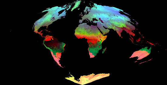
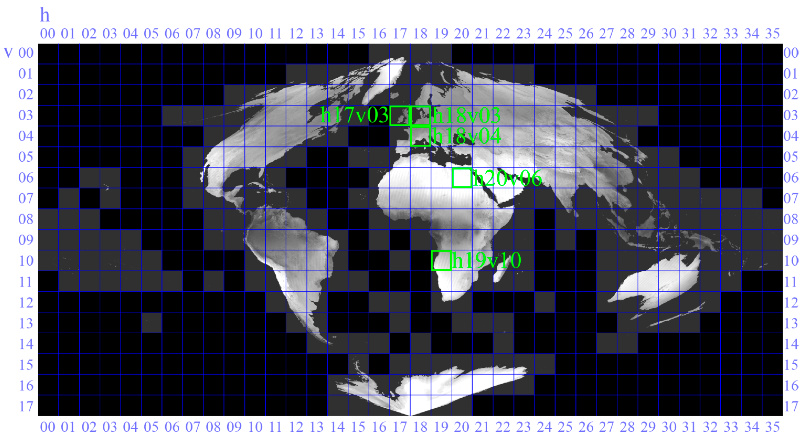
The MOD11A1 products are delivered in a sinusoidal grid by mapping the level-2 LST product (MOD11_L2) on 1 km (precisely 0.928-km) grids (Figure 1). The tiles are numbered horizontally and vertically starting at h00v00 (horizontal tile number, vertical tile number) in the upper left corner and proceeding right (horizontal) and downward (vertical). The tile size is 10° by 10° at the equator. The projection is an equal area projection and has large distortions at higher latitudes and longitudes.
The V5 MOD11A1 product’s acquisition range started 5 March 2000. For this study all acquisitions from then until the 31 December 2013 were used.
Figure 1.
Tiles and projection of MODIS land products. Tiles selected as examples for this study are highlighted.
Figure 1.
Tiles and projection of MODIS land products. Tiles selected as examples for this study are highlighted.
2.2. MODIS Land Cover and Urban Areas
The MODIS Land Cover product MCD12Q1 version 5.1 provides a classification of the global land cover in different classification systems. The land cover properties are contained within 500 m sinusoidal grids and are derived from one year of observations from the satellites Terra- and Aqua. Version 5.1 are produced with revised training data and several algorithm refinements [43]. The product contains five classification schemes with the primary land cover scheme identifying 17 land cover classes defined by the International Geosphere Biosphere Programme (IGBP). The scheme consists of 11 natural vegetation classes, three developed and mosaicked land classes, and three non-vegetated land classes. Here the IGBP classification scheme was utilized unless otherwise stated.
In this study, the land cover dataset was used to extract the surface urban heat island. Therefore, urban land cover was resampled to the 1000 m grid using nearest neighbor interpolation. Major urban centers were extracted by a morphological opening with a disk shaped structuring element of two pixel radius which means smaller urban areas (for instance, towns and villages) were excluded from the analysis. The corresponding rural areas were defined as all pixels within 15 pixels (~15 km) distance from the urban core areas that were not classified as urban in the original classification. Since only mean values for the urban and rural areas were analyzed and substantial change was not expected in the selected region (namely Great Britain), the land cover data from approximately the middle of the period (2006) were used.
2.3. Annual Cycle Parameters
The fundamental idea of ACP is the use of multi-temporal thermal data from long time periods to generate a pixel-wise simplified climatology of LST. The derived LST is applicable for acquisitions during largely cloud free conditions. Hence, every measurement is divided into a long-term average annual cycle of LST (which reflects the irradiation and climatology) as well as a day-specific anomaly (determined by meteorological, vegetation and soil conditions, as well as the exact overpass time), hereafter referred to as residuals. This climatology is periodic and hence can be approximated by a series of harmonic functions [35].
For the ACP model, the annual cycle is approximated by a constant term plus a sine function
where d is the day of the cycle and the three ACPs are the mean annual surface temperature (MAST), the yearly amplitude of surface temperature (YAST) and the phase shift θ. The phase shift accounts for the periodic boundary conditions of the surface energy balance which are shifted relatively to the radiative forcing (i.e., air temperature) and hence can be seen as a measure of the latency of heat uptake. It has to be acknowledged that between the tropic of Cancer and the tropic of Capricorn the model is less meaningful since the irradiation is characterized by two annual maxima instead of one especially at very low latitudes.
Since the ACPs were first developed for the Northern hemisphere and the larger percentage of land areas are on this hemisphere, the phase shift was defined relative to the spring equinox on 21st of March. Since a phase shift of π (respectively 182.5 days) is equivalent to a multiplication of the amplitude by −1, the YAST was set ≥ 0 per definition and the phase shift as −π ≤ θ < π respectively −182.5 days ≤ θ < 182.5 days. Since the full cycle was set to 365 days, intercalary days were ignored.
Figure 2.
Principle of the annual cycle parameters. (a) Sequence of acquisitions from tile h18v04 (covering Northern Italy, Switzerland, as well as large parts of France and Southern Germany) from different seasons (and also years); (b) Full time series for three selected pixels with different annual LST characteristics (Po Valley, Lake Garda, and Alpine mountains). (c) RGB color composite from the fitted parameters YAST, MAST and phase shift θ. Selected pixels are marked with +; (d) Annual cycle of the selected pixels and explanation of the parameters YAST, MAST, θ, and RMSE for the Alpine pixel.
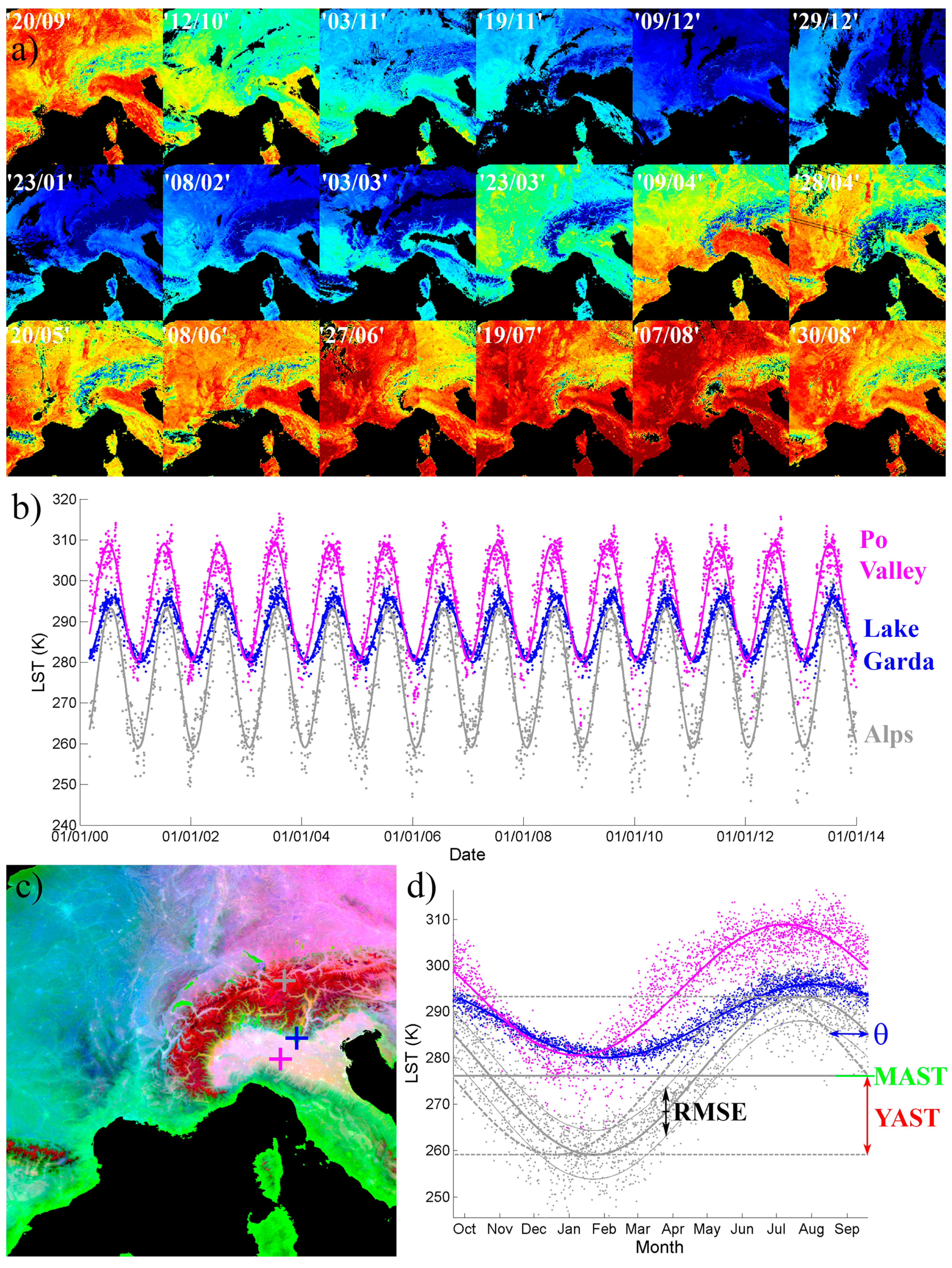
As additional parameters the root mean squared error (RMSE) of the fit and the number of clear sky acquisitions (NCSA) were calculated. Since the RMSE is the quadratic mean of the residuals, it is not only an accuracy measure but also a climatic characteristic providing an integrated measure of both the inter-diurnal and inter-annual variability of LST. NCSA on the other hand, is a measure for frequency of cloud occurrence, although it is strongly influenced by the orbital characteristics (areas in overlapping orbits have a larger number of cloud free observations). The principle is illustrated in Figure 2.
For a given series of LST measurements, the ACP for every pixel were estimated with an unconstrained nonlinear optimization algorithm [44] minimizing the square sum of the residuals. This iterative direct search method without gradients is based on a simplex (essentially an N-dimensional triangle) of parameter vectors. At each step a new point in or near the current simplex is created, its function value is compared with the function’s values at the vertices, and a new simplex of the best remaining values is created until the diameter of the simplex falls below a predefined threshold.
The minimization algorithm was already implemented in MATLAB and the ACPs were computed on a supermicro-server with 4 sockets of AMD Opteron (Abu-Dhabi) 6386 SE (4 × 16 cores, 1.4 to 2.8 GHz), 256 GB RAM, and a 100 TB external general parallel file system. Since the entire set of acquisitions (about 5000 scenes) for one tile was held in memory for processing, each tile demanded for approximately 14 GB of memory. Thus, the day and night-time ACP each took about one week of processing using 15 cores or 30 CPU-weeks in total respectively.
3. Results and Discussions
3.1. Cloud Quality Control
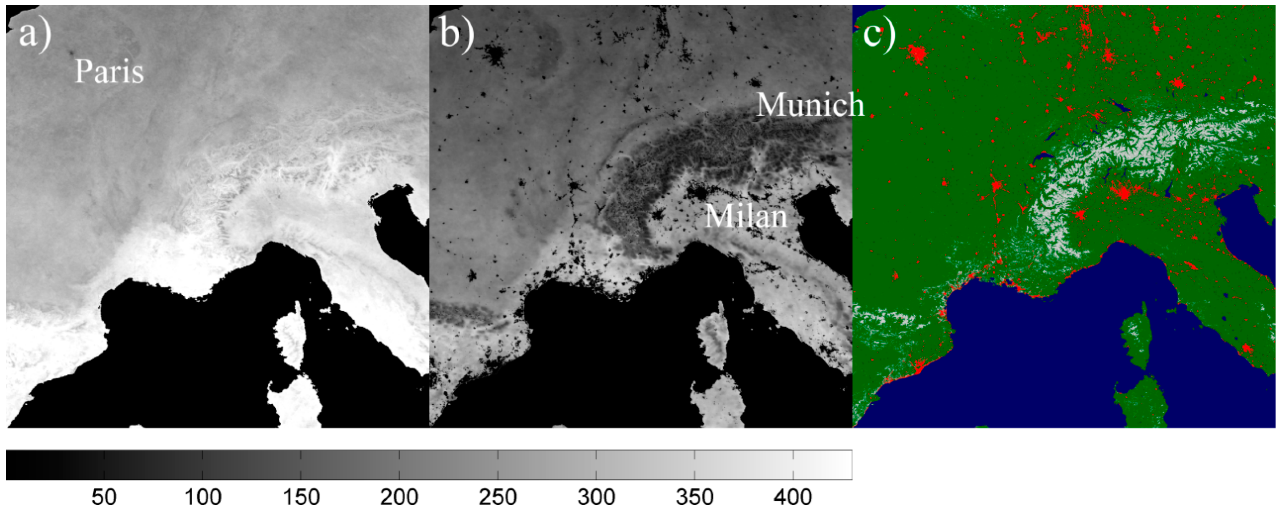
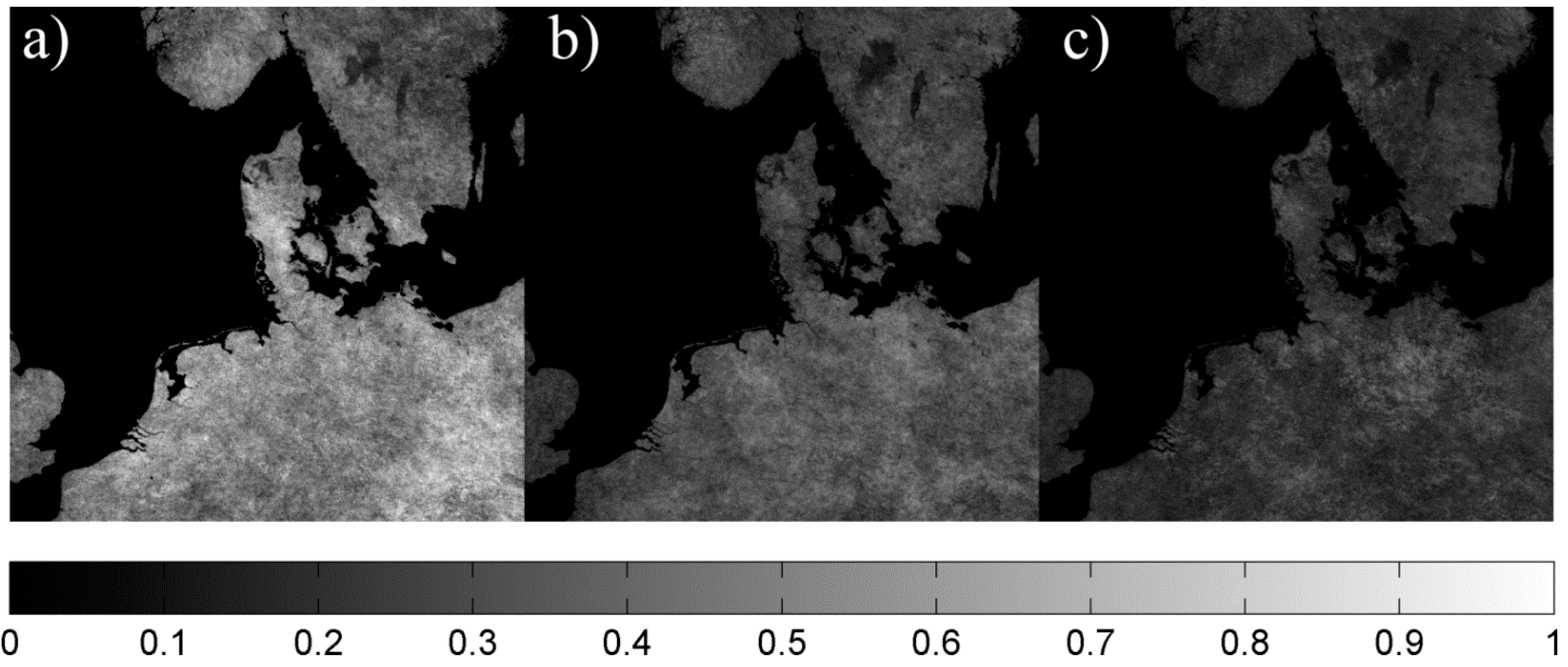
An accurate cloud masking plays an important role in the determination of multi-temporal LST parameters. Particularly, there is a tradeoff between avoidance of cloud contaminated pixels and a sufficiently large number of acquisitions for a precise fit of the model. The MOD11A1 product is already cloud filtered and delivers additional information about the quality of each produced data. The mandatory quality assessment (QA) flag within the product consists of two bits. A value of 00 indicates “LST produced, good quality, not necessary to examine detailed QA” while a value of 01 means “LST produced, unreliable or unquantifiable quality” [38]. Values of 10 and 11 mean “LST not produced due to cloud effects” and “other reasons than clouds” respectively. Hence, for this study the relevant decision was whether the unreliable or unquantifiable quality observations should be included in the ACP modelling. Figure 3 shows the number of available observations for the years 2011–2012 for MODIS tile h18v04 in total (a) and (b) with QA flag 00 only. While the number of available scenes generally decreased from an average of 231 to 131 by employing this criteria, the decrease is highly dependent on the land cover type. This especially is the case for snow and urban areas, which are frequently miss-classified as clouds or routinely not assessed as good quality. Large urban agglomerations like Paris or Milan can even be seen in the total number of produced acquisitions.
Figure 3.
Number of cloud free scenes for the period 2011–2012 for tile h18v04 for (a) all produced acquisitions; (b) acquisitions with good (“00”) quality flag; (c) Urban areas (red) according to MODIS land cover dataset.
Figure 3.
Number of cloud free scenes for the period 2011–2012 for tile h18v04 for (a) all produced acquisitions; (b) acquisitions with good (“00”) quality flag; (c) Urban areas (red) according to MODIS land cover dataset.

This selection also has implications on the quality of the accuracy of the produced ACP. Table 1 shows the mean values of the ACP produced with all acquisitions and the good acquisitions (QA = “00”) only for the same tile and period. Both, MAST and YAST are higher for the good acquisitions, which indicates a certain cloud contamination in the full dataset. Unfortunately, this variation is systematic (not displayed) with smaller differences in the Mediterranean areas (South) than in the region closer to the North Sea, which is likely related to the frequency of cloud cover and unfiltered contamination. Otherwise, the Alps (East) also show comparably high differences which are assumed to be a result of a systematic filtering of days with snow cover. Hence, it cannot inevitably be concluded that the ACP from the QA filtered product are more accurate. While for MAST both datasets are very well correlated for YAST, the R value amounts to only 0.87, which indicates that the parameter is more sensitive to outliers. The phase shift θ seems least sensitive to the selection of cloud free scenes. Since urban areas are one of the major applications of the product the entire LST data set was used without consideration of the QA flag.

Table 1.
Mean ACP for tile h18v04 for 2011–2012 for all produced values, good QA only, and correlation coefficient between both.
| Parameter | All | Good | R |
|---|---|---|---|
| YAST (K) | 12.0 | 12.6 | 0.87 |
| MAST (K) | 289.4 | 291.0 | 0.99 |
| θ | −0.35 | −0.34 | 0.95 |
3.2. Accuracy of ACP Retrieval
To assess the dependence of the accuracy on the number of available acquisitions, a bootstrapping type random experiment was conducted. Therefore, from the years 2001–2013 repeatedly scenes were randomly drawn that correspond to the expected numbers from 1, 2, and 4 years respectively. For each sample size ten different ACP sets were calculated. Figure 4 shows the spatial distribution of the standard deviation of the ten MAST values calculated from the different sets. The accuracy of the calculated parameters was seen to clearly increase with larger sample size. The median standard deviation of all pixels was 0.47 K for 1 year, 0.29 K for 2 years and 0.20 K for 4 years of data. Similarly, the median standard deviation of YAST was 0.66 K for 1 year, 0.46 K for 2 years and 0.30 K for 4 years of randomly chosen data which again shows that YAST is more sensitive towards the selection of scenes. It should be noted that the chosen sets are not entirely independent since some scenes are drawn in several sets. However, statistically the overlap between two sets was less than 1% for 1 year and still less than 10% for 4 years. On the other hand, the variability within the 13 years of data can be assumed to be higher than within one real year, hence the real accuracy may be higher. Although the 4 years of data already result in a reasonable accuracy the error due to the random selection of scenes is still considerable. Hence, it is recommended to calculate ACP from time series of several years if available. For this study, the entire period from 2000 to 2013 was used to achieve the highest possible accuracy even if this increases the computational costs.
Figure 4.
Standard deviation for MAST of 10 randomly sets of scenes equivalent to (a) one, (b) two, and (c) four years of data in Kelvin for tile h18v03.
Figure 4.
Standard deviation for MAST of 10 randomly sets of scenes equivalent to (a) one, (b) two, and (c) four years of data in Kelvin for tile h18v03.
3.3. Global Climatology of LST
Figure 5 shows some results of the global ACP modelling experiment. MAST is dominated by large scale temperature gradients. Roughly, the tropics and subtropics appear in red, temperate climates in orange, continental and especially boreal climate in green and artic climates in blue. The topography is also evident, in particular highland areas such as the Tibetan Plateau are seen as considerably colder than surrounding areas in the annual mean LST, as well as the Alps and the Andes, both of which are clearly visible.
Vegetation decreases MAST, as for instance can be seen in the areas of tropical rain forests. The pattern shows effects of the general (atmospheric) circulation such as the high LST values evident in the subtropical desserts at the down-welling edges of the Hadley cells. To a certain extent the effects of the Thermohaline (ocean) circulation can also be seen as for instance the comparably warmer temperatures in Europe than in America at comparable latitudes caused by the Gulf Stream.
Figure 5.
Results of the global ACP modelling experiment including all observations from 2000–2013. (a) Daytime mean annual surface temperature (MAST) in K; (b) Daytime yearly amplitude of surface temperature (YAST) in K; (c) Daytime phase shift θ in days; (d) Daytime RMSE of fit in K; (e) Number of daytime clear sky acquisitions (NCSA); (f) ∆MAST between day- and nighttime as measure for the amplitude of the diurnal temperature cycle in K; (g) RGB color composite of θ-RMSE-YAST; (h) Composite of MAST-NCSA-∆YASTday-night.
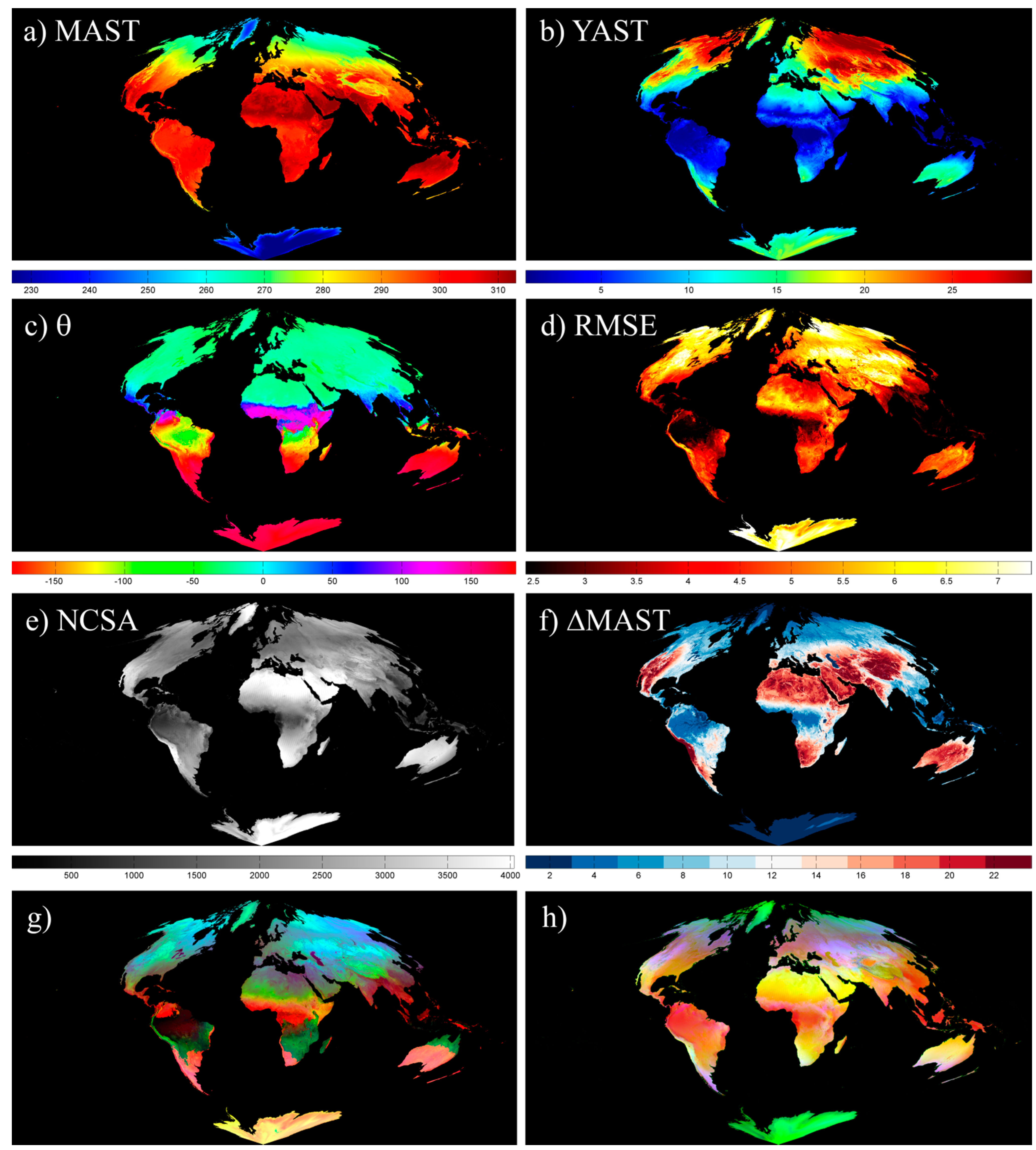
The annual amplitude YAST increases from the equator to the poles which demonstrates increasing seasonality associated with higher latitudes. Moreover YAST increases with continentality (e.g., in Siberia). The eastern parts of America and Eurasia show a more pronounced increase in YAST below the Ferrel cell, which might result from the frequent passage of Westerly disturbances and according oceanic influence in the west. Large water bodies especially at higher latitudes (e.g., Lake Baikal, Great Lakes) and river deltas (Nile, Amazon) show low YAST and partly seem to cause decreasing YAST values in the surrounding areas. Besides extreme variations in the irradiation forcing, Artic areas show smaller annual amplitude than boreal areas due to their perennial snow coverage.
The phase shift θ especially reflects the shifted seasons on the northern and southern hemispheres. In the northern hemisphere the lag (compared to the irradiation maximum) amounts to a couple of weeks and slightly increases from about 15 days at 25° N to about 29 days at 70° N. Large water bodies and high snow covered mountainous regions exhibit higher θ. Climates in low latitudes that are dominated by dry and wet seasons rather than the irradiation show a positive θ (e.g., in India and Southeast Asia, likely related to Monsoon effects). These values should be treated with caution since they result from the unequal distribution of cloud-free observations and the sine function presumably does not fit the real annual course of LST well. Nevertheless, e.g., the θ of about 50 days which was found in the Gulf of Mexico is consistent with the characteristic warmest Months April and May in Mexico-City. In the Southern hemisphere, θ is shifted by half a year and hence also a few weeks after solar irradiation. Around the equator a mixed “transition zone” with discontinuous θ can be found, however this occurs at low amplitudes. As stated above the ACP should be treated carefully between the tropics since the annual irradiation is not well approximated by the sine function at low latitudes. A general influence of the continentality cannot be detected in these regions. The noticeably increased phase shifts at the African and South American West coasts might be associated with the cold ocean currents Benguela Current and Peru Current.
The variability parameter RMSE is also increasing with latitude and likewise shows a strong impact of seasonality and continentality. Generally, the large scale RMSE pattern is mostly consistent with YAST. This makes sense, since large annual variation is likely to promote larger inter-diurnal and inter-annual variation. Further, substantial impact of land cover can be seen. Especially, tropical forests show very low variability. Otherwise, the Sahel zone shows a comparably high RMSE which is likely resulting from the high inter-annual variability.
The number of cloud free acquisitions essentially reflects the cloud climatology with the lowest values in the tropics and the highest values in sub-tropical deserts. Large rivers like Amazon and Danube and Lakes can be seen as reduced NCSA, which might either result from increased water availability for convective cloud formation or be an artefact of the cloud filtering algorithm which is likely sensitive to the water absorption spectrum.
The parameter ∆MAST denotes the difference between daytime and nighttime MAST and hence is a measure for the amplitude of the DTC. It shows low values in the tropical, boreal, and artic zones and high values in arid climates. Since the latitudinal gradient is comparably smaller for this “relative” parameter than for the absolute parameters MAST and YAST, the impact of land cover is much more pronounced. This results in a strong signal of rivers and water bodies, forest, and geology. Regarding the day-night differences of the other parameters (not displayed) YAST and RMSE generally are also lower during night which coincides with the reduced heat in the system. The phase shift is in general very similar at nighttime although the transition around the equator is a bit smoother for the nighttime acquisitions. The NCSA is generally higher during day in the tropics and higher during night in higher latitudes which might be related either to the different diurnal cloud characteristics or the acquisition schedule. It should be noted that the pattern is not useful without correction, since it is largely disturbed by the day and nighttime orbits.
If several parameters are combined as a RGB color composite the thermal landscapes can be visualized with even higher information density. Two examples are given in subfigures (g) and (h) which are RGB color composite of θ-RMSE-YAST and MAST-NCSA-∆YASTday-night respectively. Here the interpretation of the single parameters is more difficult but the composite gives a good intuitive impression of the thermal characteristics of the landscapes and the scope of the parameter set.
Besides real surface characteristics, the ACPs also contain some artefacts. As already discussed, the orbit patterns can be seen in NCSA especially at low latitudes. This inconsistency is partly inherited by RMSE since a higher number of (averaged) daily acquisitions smoothens the time series and reduces their variability. Another inconsistency can be found in NCSA and likewise in RMSE between the vertical tiles v02 and v03 in Siberia and North America especially at night-time.
Table 2 shows the correlation coefficients between the different parameter patterns (calculated from a smaller dataset which was resampled to 20% of the size). High correlations were found between YAST and RMSE due to the concurrence of high annual amplitudes and higher inter-diurnal amplitudes. The high correlations between YAST and MAST at daytime and the respective differences to the night-time values are trivial. A strong negative correlation was found between YAST and MAST due to the opposed latitudinal gradients and between YAST and RMSE which is a combined effect of the previous two. Generally, the low correlations indicate a low redundancy and high information content of the parameters. However, the small scale correlation might differ. For instance YAST and MAST show strong positive correlation at local scale where the differences are controlled by the thermal characteristics of the surface rather than differential irradiation. Hence, larger heat conductivity results in both, higher temperatures and larger diurnal and annual cycles. Consequently, the ACP must also be studied at a higher spatial scale in order to fully capture the local variation and utility of the parameters.
| R | YASTday | MASTday | thetaday | RMSEday | NCSAday | ∆YASTday-night | ∆MASTday-night |
|---|---|---|---|---|---|---|---|
| YASTday | 1.00 | −0.46 | 0.00 | 0.71 | 0.13 | 0.66 | 0.01 |
| MASTday | −0.46 | 1.00 | −0.33 | −0.54 | −0.13 | −0.10 | 0.66 |
| thetaday | 0.00 | −0.33 | 1.00 | 0.16 | 0.26 | 0.06 | −0.14 |
| RMSEday | 0.71 | −0.54 | 0.16 | 1.00 | 0.36 | 0.39 | 0.08 |
| NCSAday | 0.13 | −0.13 | 0.26 | 0.36 | 1.00 | 0.07 | 0.38 |
| ∆YASTday-night | 0.66 | −0.10 | 0.06 | 0.39 | 0.07 | 1.00 | 0.21 |
| ∆MASTday-night | 0.01 | 0.66 | −0.14 | 0.08 | 0.38 | 0.21 | 1.00 |
3.4. Thermal Landscape of Annual Cycle Characteristics
Due to the large number of more than 300 tiles and 10 parameters per tile (without combinations) only a very limited selection can be shown here. To increase the information density, color composites of 3 parameters are displayed. Figure 6 shows four such composite of single tiles. The first tile (a) shows a θ-YAST-RMSE composite of tile h18v03 which comprises mostly the Netherlands, Northern Germany as well as parts of neighbor countries. The phase shift (red) is strongest closer to the North Sea and in snow covered parts of Norway. YAST (green) is higher in Scandinavia and the East which indicates the increasing seasonality with latitude and continentality. The RMSE (blue) also shows a gradient from west to east (only partly visible in the composite). Urban areas are clearly distinguishable in yellow which somewhat resembles nightlight imagery.
Figure 6.
Selected ACP color composite of single tiles (hxxvyy) (a) θ-YAST-RMSE of (h18v03); (b) Nighttime RMSE-YAST-θ (h18v04); (c) RMSE-MAST-YAST (h20v06); (d) MAST-YAST-RMSE (h19v10).
Figure 6.
Selected ACP color composite of single tiles (hxxvyy) (a) θ-YAST-RMSE of (h18v03); (b) Nighttime RMSE-YAST-θ (h18v04); (c) RMSE-MAST-YAST (h20v06); (d) MAST-YAST-RMSE (h19v10).
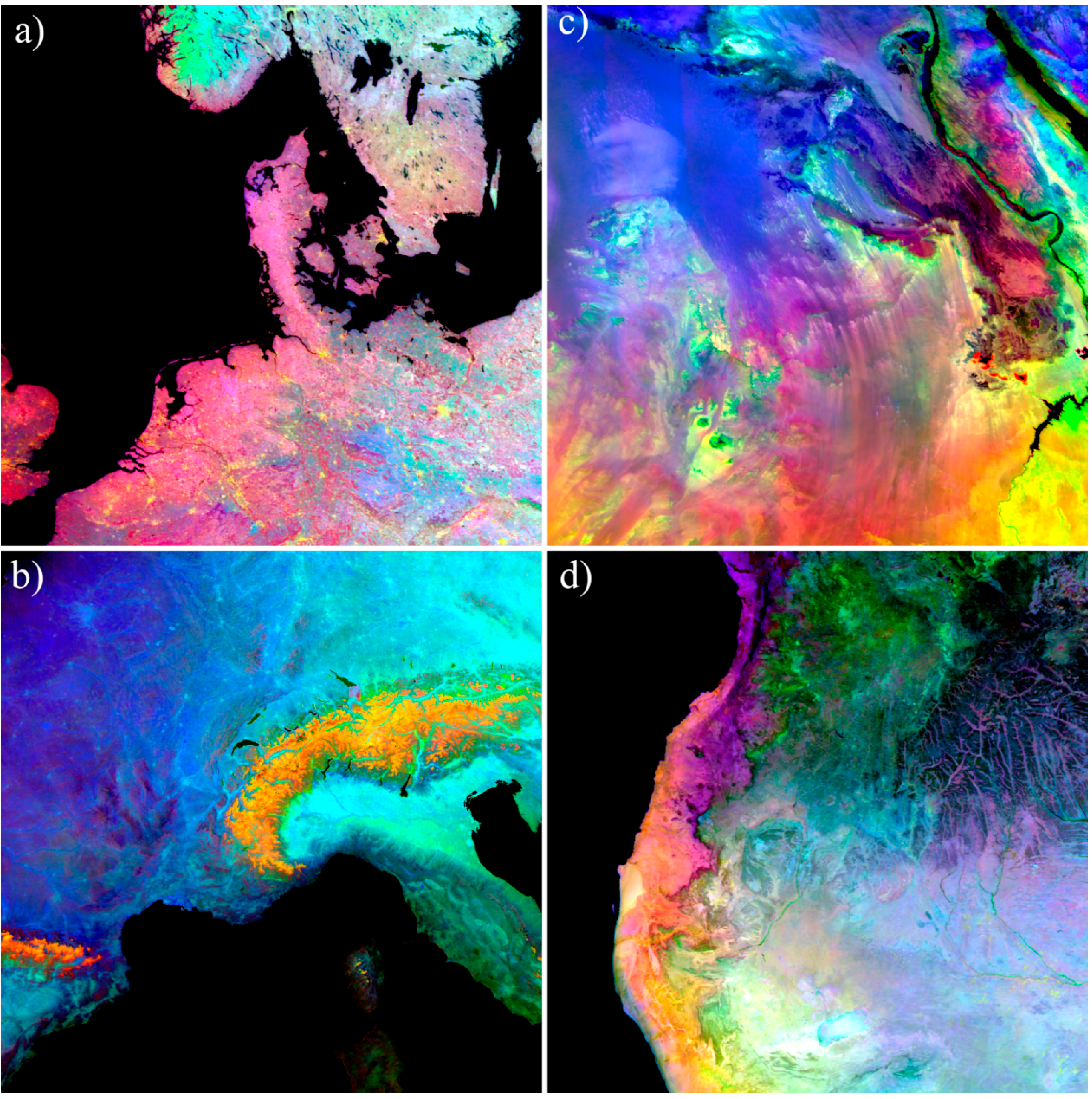
The second composite (b) is the adjacent tile to the south encompassing Northern Italy, Switzerland, as well as large parts of France and Southern Germany. This is a composite of three nighttime parameters, namely RMSE, YAST and θ. The (inter-diurnal and inter-annual) variation is especially high in the Alps and the Pyrenees which likely is an effect of different snow covers. The annual amplitude (green) shows a gradient from west to east with substantially larger values in the Po Valley south of it. MAST (blue) is lowest in the high mountainous regions (which together with the high RMSE results in the yellow color) and shows a strong gradient from the North towards the Mediterranean coast. Again, MAST shows a substantial impact of urban areas, most prominently the metropolitan region of Paris in the upper left of the image.
The third tile (c) shows a composite of RMSE, MAST and YAST of the Nile delta (upper left) and parts of the Sahara which mostly belong to Egypt as well as partly to Libya and Sudan. The delta is clearly visible in green while the rest of the composite is dominated by the geology which also leaves a large fingerprint in the diurnal differences (not shown). RMSE contains slight artefacts of NCSA in Northern Africa which can be seen as stripes in the upper left.
Tile (d) shows the West coast of Southern Africa with Angola in the north and Namibia in the south. The composite of daytime MAST, YAST and RMSE shows strong mean values (red) in the desert in the West, lower values in Kalahari Basin east of it, and much lower values in the Savannas in the north. The amplitude shows a strong gradient from north to south (green). While at the coastline geological influences can be seen, in the north-east the source areas of the Okavango (although not the delta) are very pronounced. The Etosha pan inside the Kalahari Basin can be recognized as homogenous very light blue area in the south.
3.5. Urban Climatology: A New Way of Mapping the Surface Urban Heat Island
The urban heat island (UHI) is of large interest and has been investigated over decades [45,46]. Thermal imagery plays a key role in UHI assessment. It offers the chance to directly measure the surface temperature which is crucial for the urban energy balance and modulates the air temperature of the lowest atmospheric layer. Further, the spatial structure of the surface temperature patterns is directly related to surface characteristics and also used to study the energy balance and the relation between atmospheric and surface UHI (SUHI). However, only the SUHI can be directly observed and there are various problems [7] but also progress [47,48,49] involved in estimating air temperatures from TIR data. Another common shortcoming of remote sensing SUHI studies is that they are frequently based on a single or a few acquisitions only and hence are strongly influenced by actual meteorological and soil conditions. If for instance clouds have shaded the ground before the observation this might result in substantial gradients which cannot easily be interpreted or eliminated. Since the ACP provides LST characteristics from a very large number of acquisitions they might be seen as a new paradigm for SUHI studies, as they allow researchers to analyze the effect and its annual course independent of clouds and instantaneous surface conditions. Further, the analysis can easily be conducted not only for a single city but for larger areas at once.
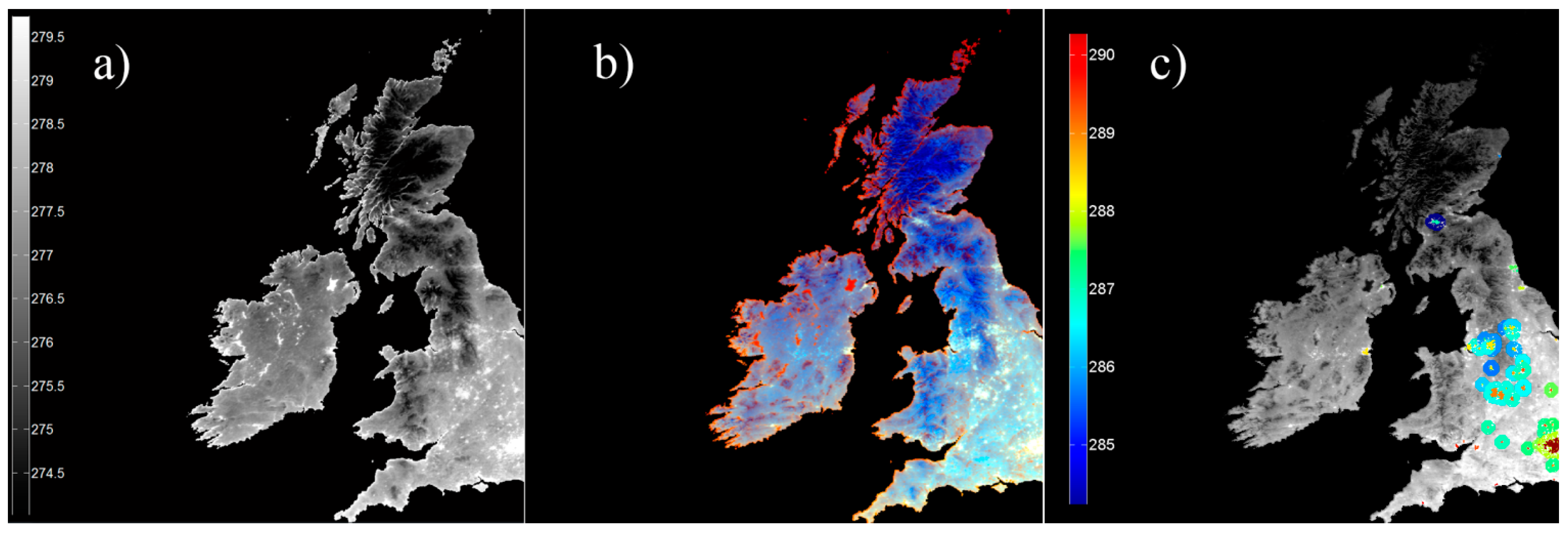
Figure 7 shows an example for Great Britain. The first image displays nighttime MAST and the second a composite of nighttime MAST, daytime MAST, and ∆MASTday-night. Urban areas are clearly visible due to their high values in all three parameters. Besides, coastlines also show high values of nighttime MAST due to the large heat capacity of the adjacent water bodies. Figure 7c shows the daytime SUHI average values for the urban centers (according to the MODIS land cover data) and the average values for the surrounding areas (defined by a 15 km buffer without any urban pixels). All cities show clear mean annual daily SUHIs with the largest effect in London. Likewise, cities show greater YAST (not displayed) but also smaller (absolute) phase shift, which indicates that no heat storage in the urban fabric for periods longer than the diurnal cycle can be seen in the parameter.
Figure 7.
Results of the surface urban heat island analysis for Great Britain. (a) Nighttime MAST; (b) Composite of nighttime MAST, daytime MAST, and ∆MASTday-night; (c) Daytime surface urban heat island of metropolitan areas. Mean MAST of urban and surrounding non-urban area.
Figure 7.
Results of the surface urban heat island analysis for Great Britain. (a) Nighttime MAST; (b) Composite of nighttime MAST, daytime MAST, and ∆MASTday-night; (c) Daytime surface urban heat island of metropolitan areas. Mean MAST of urban and surrounding non-urban area.
Since the urban extents from the MODIS mask are smaller than they would be estimated from the thermal landscape, ACP could possibly also improve urban mapping. Similarly, is has been demonstrated before that ACP are useful for the classification of intra-urban structural types like local climate zones [50,51]. However, urban areas are only one example and the global ACP dataset can be used for mapping purposes for different land covers.
3.6. Land Cover Mapping and Effective Climate Classification
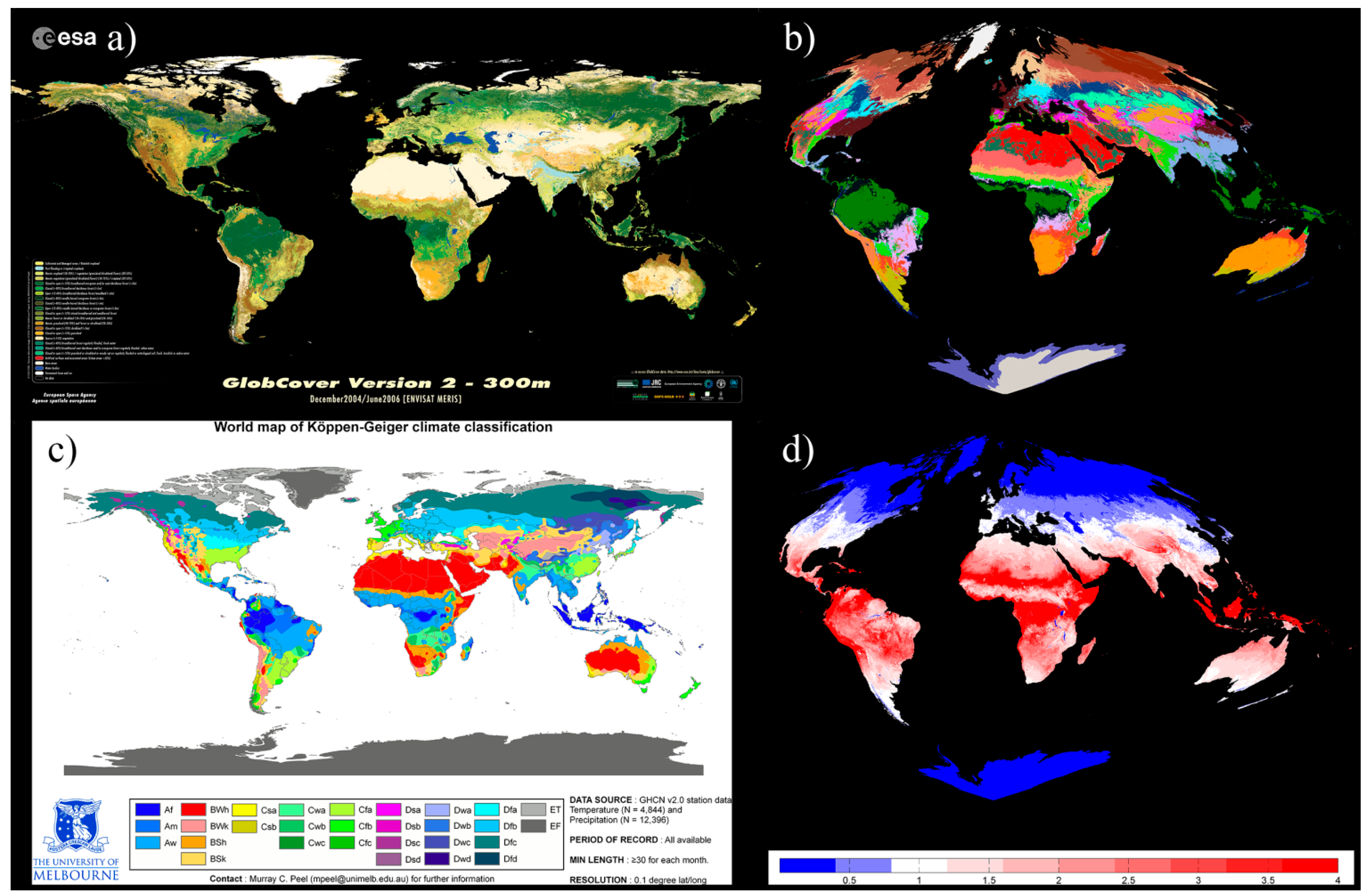
Thermal data is rarely included in global land cover mapping methods due to cloud gaps and its high temporal variability between subsequent acquisitions. Since they provide a robust long term estimate this is not the case for the ACPs. To get an initial indication of their utility for land cover mapping, a k-means cluster analysis (k = 30) of selected normalized ACPs (day: YAST, MAST, RMSE and NCSA; night: YAST, MAST as well as ∆MAST) was conducted. The ESA land cover map (Figure 8a) corresponds well with the result (Figure 8b in mostly random colors) although the classification algorithm is unsupervised and hence the class borders are not necessarily consistent with real classes. However, this does not necessarily mean that the land cover determines the LST characteristics since the large scale land cover also strongly reflects the climatic conditions. Hence, the classification likewise shows similarities (but also distinct differences) with the effective climate classification in Figure 8c, which is based on in situ observations. Since such temperature observations are sparse in some regions, they are frequently interpolated using LST [52,53]. Therefore, the ACPs could also be of added value since they provide a gap-free virtual LST pattern for every day of the year. Figure 8d shows the ratio between ∆MAST and YAST as measure for diurnal (red) and seasonal (blue) climates.
Since the ACP are clearly affected by both climate and land cover they might have potential to contribute to respective classifications, but this will require further investigations of the most useful parameters and algorithms.
Figure 8.
(a) ESA GlobCover. Map may be used freely, © ESA/ESA GlobCover Project, MEDIAS France/Postel; (b) k-means clustering of ACP with 30 clusters in random color-map; (c) Effective climate classification after Köppen & Geiger by Murrat Peal and colleagues [54] © CC BY-SA 3.0 (d) diurnal (red) and seasonal (blue) climates.
4. Conclusions
In this study a new global dataset of annual land surface temperature based on MODIS LST on 1 km resolution was presented and potential applications were highlighted. The ACPs: YAST, MAST, θ, RMSE, and NCSA for daytime and nighttime were calculated from all acquisitions from MODIS/Terra from 2000 to 2013. The parameters provide a new climatology of the important Earth system parameter LST, and characterize the thermal landscape extensively and free of cloud gaps. More specifically, they allow estimating the LST patterns at different scales for every place on Earth and for every day in the year and additionally deliver an estimate of the accuracy of both inter-diurnal and inter-annual variability. The parameters are robust, but the LST estimates are limited to acquisition times and largely cloud free conditions. If cloud free conditions are unlikely to occur, for example in wet seasons, the estimated LST must be treated with caution. Furthermore, between the tropics the validity of the ACP is limited since the annual cycle of irradiation is not well approximated by the sine function at low latitudes. The accuracy due to the random selection of scenes was tested and it was found that several years of data should ideally be used. The MODIS time series is certainly long enough to provide sufficient data to achieve a high accuracy. However, this might result in errors for areas that underwent land cover change. Despite a few artefacts from the orbit characteristics and level 3 product processing, the parameters generally reflect real surface conditions. The analyses correlations between most parameters indicated their high information content and low redundancy.
The parameters revealed different important influencing factors including climate, land cover, vegetation phenology, anthropogenic effects, and geology. Accordingly, the number and scope of potential applications are various and only a few could briefly be highlighted in this study. Besides the classification of local climate zones that was already tested, ACP could also be used for classification of land cover, geology, or effective climate zones. Further, they have been found to be good predictors for the LST downscaling of LST [26,55] and they could be used for change detection if the thermal characteristics show discontinuous or systematic deviations. Finally, a comprehensive evaluation of global SUHIs based on the ACP is currently conducted.
Since the parameters now have reached a stable level and are assumed to be of use for several applications, testers and applicants are welcome. After final processing the ACP datasets will published at the CliSAP Integrated Climate Data Center [56]—until then please contact the author. Besides, future work will include improvements of the parameters. This might include a more detailed analysis of the residuals and their temporal distribution to distinguish varying inter-daily variability in different seasons, inter-annual variability throughout the years, the effect of the seasonal cloud distribution, as well as systematic changes. Moreover, better cloud filtering by using neighborhood relations or excluding outliers in an iterative algorithm could improve the cloud-free fit and might even allow estimations of LST at conditions with a certain amount of convective clouds. A more detailed analysis of the QA flags and their dependency on land cover and LST also deserves further attention. However in this regard, it might make sense to wait for future anticipated products. For instance, version 6 of MOD11A1 will be available in the near future. This also applies to the new MOD21 product, which is based on a temperature emissivity separation algorithm with the MODIS bands 29, 31, and 32 [57,58]. Besides, the respective Aqua product MYD11A1 is currently processed which will increase the climatology to four times a day and will already allow for some DTC analysis.
Acknowledgments
I thank all data providers, especially the NASA and the USGS. Further, I thank Eleonore Schenk and Jürgen Böhner for acquisition and access to the computing resources as well as Thomas Orgis and Hinnerk Stüben for technical support. Eventually, I want to thank Manfred Bechtel, Lars Gerlitz, and Paul Alexander for proof reading as well as Otto Bechtel for his dedicated overall help with my work. This work was financed by the Cluster of Excellence CliSAP (EXC 177), University of Hamburg funded through the German Science Foundation (DFG).
Conflicts of Interest
The author declares no conflict of interest.
References
- Dash, P.; Göttsche, F.-M.; Olesen, F.-S.; Fischer, H. Land surface temperature and emissivity estimation from passive sensor data: Theory and practice-current trends. Int. J. Remote Sens. 2002, 23, 2563–2594. [Google Scholar]
- Li, Z.-L.; Tang, B.-H.; Wu, H.; Ren, H.; Yan, G.; Wan, Z.; Trigo, I.F.; Sobrino, J.A. Satellite-derived land surface temperature: Current status and perspectives. Remote Sens. Environ. 2013, 131, 14–37. [Google Scholar]
- Bastiaanssen, W.G.M.; Menenti, M.; Feddes, R.A.; Holtslag, A.A.M. A remote sensing surface energy balance algorithm for land (SEBAL). 1. Formulation. J. Hydrol. 1998, 212, 198–212. [Google Scholar]
- Frey, C.M.; Parlow, E. Flux measurements in Cairo. Part 2: On the determination of the spatial radiation and energy balance using ASTER satellite data. Remote Sens. 2012, 4, 2635–2660. [Google Scholar]
- Kalma, J.D.; McVicar, T.R.; McCabe, M.F. Estimating land surface evaporation: A review of methods using remotely sensed surface temperature data. Surv. Geophys. 2008, 29, 421–469. [Google Scholar]
- Li, Z.; Jia, L.; Lu, J. On uncertainties of the Priestley-Taylor/LST-Fc feature space method to estimate evapotranspiration: Case study in an arid/semiarid region in Northwest China. Remote Sens. 2014, 7, 447–466. [Google Scholar]
- Voogt, J.A.; Oke, T.R. Thermal remote sensing of urban climates. Remote Sens. Environ. 2003, 86, 370–384. [Google Scholar]
- Weng, Q. Thermal infrared remote sensing for urban climate and environmental studies: Methods, applications, and trends. ISPRS J. Photogramm. Remote Sens. 2009, 64, 335–344. [Google Scholar]
- Fabrizi, R.; Bonafoni, S.; Biondi, R. Satellite and ground-based sensors for the urban heat island analysis in the city of Rome. Remote Sens. 2010, 2, 1400–1415. [Google Scholar]
- Liu, L.; Zhang, Y. Urban heat island analysis using the Landsat TM data and ASTER data: A case study in Hong Kong. Remote Sens. 2011, 3, 1535–1552. [Google Scholar]
- Prata, A.J.; Caselles, V.; Coll, C.; Sobrino, J.A.; Ottle, C. Thermal remote sensing of land surface temperature from satellites: Current status and future prospects. Remote Sens. Rev. 1995, 12, 175–224. [Google Scholar]
- Sobrino, J.A.; Jiménez-Muñoz, J.C.; Paolini, L. Land surface temperature retrieval from LANDSAT TM 5. Remote Sens. Environ. 2004, 90, 434–440. [Google Scholar]
- Qin, Z.; Karnieli, A.; Berliner, P. A mono-window algorithm for retrieving land surface temperature from Landsat TM data and its application to the Israel-Egypt border region. Int. J. Remote Sens. 2001, 22, 3719–3746. [Google Scholar]
- Jimenez-Munoz, J.C.; Sobrino, J.A. A single-channel algorithm for land-surface temperature retrieval from ASTER data. IEEE Geosci. Remote Sens. Lett. 2010, 7, 176–179. [Google Scholar]
- Sobrino, J.A.; Li, Z.-L.; Stoll, M.P.; Becker, F. Multi-channel and multi-angle algorithms for estimating sea and land surface temperature with ATSR data. Int. J. Remote Sens. 1996, 17, 2089–2114. [Google Scholar]
- Price, J.C. Land surface temperature measurements from the split window channels of the NOAA 7 advanced very high resolution radiometer. J. Geophys. Res. Atmos. 1984, 89, 7231–7237. [Google Scholar]
- Wan, Z.; Dozier, J. A generalized split-window algorithm for retrieving land-surface temperature from space. IEEE Trans. Geosci. Remote Sens. 1996, 34, 892–905. [Google Scholar]
- Berk, A.; Anderson, G.P.; Bernstein, L.S.; Acharya, P.K.; Dothe, H.; Matthew, M.W.; Adler-Golden, S.M.; Chetwynd, J.H.J.; Richtmeier, S.C.; Pukall, B.; et al. MODTRAN4 radiative transfer modeling for atmospheric correction. Proc. SPIE 1999, 3756, 348–353. [Google Scholar]
- Snyder, W.C.; Wan, Z.; Zhang, Y.; Feng, Y.Z. Classification-based emissivity for land surface temperature measurement from space. Int. J. Remote Sens. 1998, 19, 2753–2774. [Google Scholar]
- Valor, E.; Caselles, V. Mapping land surface emissivity from NDVI: Application to European, African, and South American areas. Remote Sens. Environ. 1996, 57, 167–184. [Google Scholar]
- Sobrino, J.A.; Jiménez-Muñoz, J.C.; Sòria, G.; Romaguera, M.; Guanter, L.; Moreno, J.; Plaza, A.; Martínez, P. Land surface emissivity retrieval from different VNIR and TIR sensors. IEEE Trans. Geosci. Remote Sens. 2008, 46, 316–327. [Google Scholar]
- Gillespie, A.; Rokugawa, S.; Matsunaga, T.; Cothern, J.S.; Hook, S.; Kahle, A.B. A temperature and emissivity separation algorithm for Advanced Spaceborne Thermal Emission and Reflection radiometer (ASTER) images. IEEE Trans. Geosci. Remote Sens. 1998, 36, 1113–1126. [Google Scholar]
- Tomlinson, C.J.; Chapman, L.; Thornes, J.E.; Baker, C. Remote sensing land surface temperature for meteorology and climatology: A review. Meteorol. Appl. 2011, 18, 296–306. [Google Scholar]
- Inamdar, A.K.; French, A.; Hook, S.; Vaughan, G.; Luckett, W. Land surface temperature retrieval at high spatial and temporal resolutions over the southwestern United States. J. Geophys. Res. 2008, 113. [Google Scholar] [CrossRef]
- Zakšek, K.; Oštir, K. Downscaling land surface temperature for urban heat island diurnal cycle analysis. Remote Sens. Environ. 2012, 117, 114–124. [Google Scholar]
- Bechtel, B.; Zakšek, K.; Hoshyaripour, G. Downscaling land surface temperature in an urban area: A case study for Hamburg, Germany. Remote Sens. 2012, 4, 3184–3200. [Google Scholar]
- Chen, X.; Li, W.; Chen, J.; Rao, Y.; Yamaguchi, Y. A combination of TsHARP and thin plate spline interpolation for spatial sharpening of thermal imagery. Remote Sens. 2014, 6, 2845–2863. [Google Scholar]
- Keramitsoglou, I. Advanced earth observation methodologies for the study of the thermal environment of cities. In Proceedings of the 2012 Second International Workshop on Earth Observation and Remote Sensing Applications (EORSA), Shanghai, China, 8–11 June 2012; pp. 11–15.
- Lu, L.; Venus, V.; Skidmore, A.; Wang, T.; Luo, G. Estimating land-surface temperature under clouds using MSG/SEVIRI observations. Int. J. Appl. Earth Obs. Geoinf. 2011, 13, 265–276. [Google Scholar]
- Göttsche, F.-M.; Olesen, F.S. Modelling of diurnal cycles of brightness temperature extracted from METEOSAT data. Remote Sens. Environ. 2001, 76, 337–348. [Google Scholar]
- Göttsche, F.M.; Olesen, F.S. Modelling the effect of optical thickness on diurnal cycles of land surface temperature. Remote Sens. Environ. 2009, 113, 2306–2316. [Google Scholar]
- Duan, S.-B.; Li, Z.-L.; Wang, N.; Wu, H.; Tang, B.-H. Evaluation of six land-surface diurnal temperature cycle models using clear-sky in situ and satellite data. Remote Sens. Environ. 2012, 124, 15–25. [Google Scholar]
- Zhou, J.; Chen, Y.; Zhang, X.; Zhan, W. Modelling the diurnal variations of urban heat islands with multi-source satellite data. Int. J. Remote Sens. 2013, 34, 7568–7588. [Google Scholar]
- Bechtel, B. Multitemporal Landsat data for urban heat island assessment and classification of local climate zones. In Proceedings of the 2011 Joint Urban Remote Sensing Event (JURSE), Munich, Germany, 11–13 April 2011; pp. 129–132.
- Bechtel, B. Robustness of annual cycle parameters to characterize the urban thermal landscapes. IEEE Geosci. Remote Sens. Lett. 2012, 9, 876–880. [Google Scholar]
- Weng, Q.; Fu, P. Modeling annual parameters of clear-sky land surface temperature variations and evaluating the impact of cloud cover using time series of Landsat TIR data. Remote Sens. Environ. 2014, 140, 267–278. [Google Scholar]
- Bechtel, B. Die Hitze in der Stadt Verstehen—Wie sich Die Jahreszeitliche Temperaturdynamik von Städten aus Dem All Beobachten Lässt. In Globale Urbanisierung—Perspektive aus dem All; Taubenböck, H., Wurm, M., Esch, T., Dech, S., Eds.; Springer Spektrum: Berlin, Germany, 2015; in press. [Google Scholar]
- Wan, Z. Collection-5 MODIS Land Surface Temperature Products Users’ Guide; University of California: Santa Barbara, CA, USA, 2007. [Google Scholar]
- Wan, Z. New refinements and validation of the MODIS Land-Surface Temperature/Emissivity products. Remote Sens. Environ. 2008, 112, 59–74. [Google Scholar]
- Wan, Z.; Zhang, Y.; Zhang, Q.; Li, Z.-L. Quality assessment and validation of the MODIS global land surface temperature. Int. J. Remote Sens. 2004, 25, 261–274. [Google Scholar]
- Wang, K.; Liang, S. Evaluation of ASTER and MODIS land surface temperature and emissivity products using long-term surface longwave radiation observations at SURFRAD sites. Remote Sens. Environ. 2009, 113, 1556–1565. [Google Scholar]
- Wan, Z. New refinements and validation of the collection-6 MODIS land-surface temperature/emissivity product. Remote Sens. Environ. 2014, 140, 36–45. [Google Scholar]
- Friedl, M.A.; Sulla-Menashe, D.; Tan, B.; Schneider, A.; Ramankutty, N.; Sibley, A.; Huang, X. MODIS Collection 5 global land cover: Algorithm refinements and characterization of new datasets. Remote Sens. Environ. 2010, 114, 168–182. [Google Scholar]
- Lagarias, J.; Reeds, J.; Wright, M.; Wright, P. Convergence properties of the Nelder—Mead simplex method in low dimensions. SIAM J. Optim. 1998, 9, 112–147. [Google Scholar]
- Yow, D.M. Urban heat islands: Observations, impacts, and adaptation. Geogr. Compass 2007, 1, 1227–1251. [Google Scholar]
- Arnfield, A.J. Two decades of urban climate research: A review of turbulence, exchanges of energy and water, and the urban heat island. Int. J. Climatol. 2003, 23, 1–26. [Google Scholar]
- Bechtel, B.; Wiesner, S.; Zaksek, K. Estimation of dense time series of urban air temperatures from multitemporal geostationary satellite data. IEEE J. Sel. Top. Appl. Earth Obs. Remote Sens. 2014, 7, 4129–4137. [Google Scholar]
- Nichol, J.E.; Fung, W.Y.; Lam, K.; Wong, M.S. Urban heat island diagnosis using ASTER satellite images and “in situ”air temperature. Atmos. Res. 2009, 94, 276–284. [Google Scholar]
- Pichierri, M.; Bonafoni, S.; Biondi, R. Satellite air temperature estimation for monitoring the canopy layer heat island of Milan. Remote Sens. Environ. 2012, 127, 130–138. [Google Scholar]
- Bechtel, B.; Daneke, C. Classification of local climate zones based on multiple earth observation data. IEEE J. Sel. Top. Appl. Earth Obs. Remote Sens. 2012, 5, 1191–1202. [Google Scholar]
- Bechtel, B.; Alexander, P.J.; Böhner, J.; Ching, J.; Conrad, O.; Feddema, J.; Mills, G.; See, L.; Stewart, I. Mapping local climate zones for a worldwide database of the form and function of cities. ISPRS Int. J. Geo-Inf. 2015, 4, 199–219. [Google Scholar]
- Prihodko, L.; Goward, S.N. Estimation of air temperature from remotely sensed surface observations. Remote Sens. Environ. 1997, 60, 335–346. [Google Scholar]
- Cresswell, M.P.; Morse, A.P.; Thomson, M.C.; Connor, S.J. Estimating surface air temperatures, from Meteosat land surface temperatures, using an empirical solar zenith angle model. Int. J. Remote Sens. 1999, 20, 1125–1132. [Google Scholar]
- Peel, M.C.; Finlayson, B.L.; McMahon, T.A. Updated world map of the Köppen-Geiger climate classification. Hydrol. Earth Syst. Sci. 2007, 11, 1633–1644. [Google Scholar]
- Bechtel, B.; Böhner, J.; Zakšek, K.; Wiesner, S. Downscaling of diurnal land surface temperature cycles for urban heat island monitoring. In Proceedings of the Urban Remote Sensing Event (JURSE), Sao Paulo, Brazil, 21–23 April 2013.
- CliSAP Integrated Climate Data Center. Available online: http://icdc.zmaw.de/modis_lst_annualcycle.html (accessed on 31 December 2014).
- Hulley, G.C.; Hook, S.J. Generating consistent land surface temperature and emissivity products between ASTER and MODIS data for earth science research. IEEE Trans. Geosci. Remote Sens. 2011, 49, 1304–1315. [Google Scholar]
- Hulley, G.; Hook, S.; Hughes, T. Moderate Resolution Imaging Spectroradiometer (MODIS) MOD21 Land Surface Temperature and Emissivity Algorithm Theoretical Basis Document. Available online: http://lst.jpl.nasa.gov/emissivity.jpl.nasa.gov/downloads/examples/documents/MOD21_LSTE_ATBD_Hulley_v2.1.pdf (accessed on 31 December 2014).
© 2015 by the authors; licensee MDPI, Basel, Switzerland. This article is an open access article distributed under the terms and conditions of the Creative Commons Attribution license (http://creativecommons.org/licenses/by/4.0/).
Share and Cite
MDPI and ACS Style
Bechtel, B. A New Global Climatology of Annual Land Surface Temperature. Remote Sens. 2015, 7, 2850-2870. https://doi.org/10.3390/rs70302850
AMA Style
Bechtel B. A New Global Climatology of Annual Land Surface Temperature. Remote Sensing. 2015; 7(3):2850-2870. https://doi.org/10.3390/rs70302850
Chicago/Turabian StyleBechtel, Benjamin. 2015. "A New Global Climatology of Annual Land Surface Temperature" Remote Sensing 7, no. 3: 2850-2870. https://doi.org/10.3390/rs70302850