Article

Development of a New Daily-Scale Forest Fire Danger Forecasting System Using Remote Sensing Data

by
Ehsan H. Chowdhury
and
Quazi K. Hassan
*
Department of Geomatics Engineering, Schulich School of Engineering, University of Calgary, 2500 University Dr NW, Calgary, AB T2N 1N4, Canada
*
Author to whom correspondence should be addressed.
Remote Sens. 2015, 7(3), 2431-2448; https://doi.org/10.3390/rs70302431
Submission received: 23 December 2014 / Revised: 11 February 2015 / Accepted: 17 February 2015 / Published: 2 March 2015

Abstract

:
Forest fires are a critical natural disturbance in most of the forested ecosystems around the globe, including the Canadian boreal forest where fires are recurrent. Here, our goal was to develop a new daily-scale forest fire danger forecasting system (FFDFS) using remote sensing data and implement it over the northern part of Canadian province of Alberta during 2009–2011 fire seasons. The daily-scale FFDFS was comprised of Moderate Resolution Imaging Spectroradiometer (MODIS)-derived four-input variables, i.e., 8-day composite of surface temperature (TS), normalized difference vegetation index (NDVI), and normalized multiband drought index (NMDI); and daily precipitable water (PW). The TS, NMDI, and NDVI variables were calculated during i period and PW during j day and then integrated to forecast fire danger conditions in five categories (i.e., extremely high, very high, high, moderate, and low) during j + 1 day. Our findings revealed that overall 95.51% of the fires fell under “extremely high” to “moderate” danger classes. Therefore, FFDFS has potential to supplement operational meteorological-based forecasting systems in between the observed meteorological stations and remote parts of the landscape.

1. Introduction

Forest fires are a critical natural disturbance in most of the forested ecosystems around the globe including the Canadian boreal forest (that represents about 10% of the global forest [1]). In fact, Canadian forests have experienced about 8300 fires that burned an average of 2.3 million ha every year for the last 25 years [1]. In general, the forest fires are usually perceived as a threat (e.g., creating health hazards, burning vegetation increasing the carbon dioxide released into the atmosphere, economic loss, etc.) [2]. However, it has many positive impacts, such as helping forest regeneration, enriching soil nutrient regimes, killing insects and diseases, etc. [3,4]. In order to suppress fires, Canada has spent in the range of CAD $500 million to $1 billion every year on average during the last decade [1]. In addition, factors like deforestation, land use change, and climate change have caused increases in both the frequency and severity of forest fires across the world [5,6] which means that understanding of fire danger conditions is very important to aid sustainable fire management strategies [7].
Currently, Canada uses the Fire Weather Index (FWI) module of the Canadian Forest Fire Danger Rating System (CFFDRS) to forecast fire danger conditions at daily scale [8]. The FWI uses a set of meteorological input variables, such as mid-day (12 pm) measurements of air temperature (Ta), wind speed, and relative humidity (RH); and 24-h cumulative rainfall acquired at point locations. This system is also used in other places (i.e., Argentina [9]; Alaska, USA [10]; Indonesia [11]; Malaysia [11]; Mexico [12]; New Zealand [13]; Portugal [14]; Spain [15]; and Sweden [16]) around the world. Despite the global acceptance of the FWI, it has an inherent problem in delineating the spatial dynamics of the danger conditions, as it employs geographic information system (GIS)-based interpolation techniques. Note that the application of various interpolation techniques (e.g., spline, kriging, inverse distance weighting) may potentially generate contrasting spatial extents even employing the same input datasets [17]. Also, in some recent studies [18,19], the statistical Numerical Weather Prediction model has been used to calculate the danger-related indices of the Canadian CFFDRS and the US National Fire Danger Rating System (NFDRS) at a spatial resolution of 1° × 1° (i.e., ~110 × 110 km2) over the boreal forested regions of Alaska, where the major issue again is the relatively low spatial resolution. In this respect, remote sensing platforms are quite often useful in acquiring data at an improved spatial resolution (i.e., 250 to 1000 m for Moderate Resolution Imaging Spectroradiometer (MODIS) in particular) in a timely manner, and have already been proven to be an effective method of monitoring and forecasting fire danger conditions [20,21,22].
In comprehending fire danger conditions, researchers have used remote sensing-derived variables during the last several decades, which can be broadly clustered into four categories. Those include: (i) meteorological variables, e.g., surface temperature (TS) [23,24], Ta [25], RH [25]; (ii) vegetation greenness, e.g., normalized difference vegetation index (NDVI) [26]; enhanced vegetation index (EVI) [27,28], relative greenness (RG) [24], visible atmospherically resistant index (VARI) [29]; (iii) surface wetness conditions, e.g., temperature-vegetation dryness index (TVDI) [30], NDVI/TS [31], TS/EVI [32]; and (iv) vegetation wetness conditions, e.g., normalized multiband drought index (NMDI) [33], normalized difference water index (NDWI) [34], normalized difference infrared index (NDII) [35,36], global vegetation moisture index (GVMI) [36]. In most of these studies, the fire danger conditions are being described either during or after the fire occurrences, meaning they cannot be used for forecasting purposes [37]. However, a limited number of studies found in the literature can be useful in forecasting. For example:
  • Vidal and Devaux-Ros [38] employed Landsat TM images to calculate TS and NDVI in conjunction with meteorological station-based Ta data to calculate the water deficit index (WDI) over the Les Maures Mediterranean forests in southern France during 1990–1992 and observed that 100% of the fire pixels were captured in location where the pre-fire WDI value was ≥0.6. The major weakness of the study was the use of only 3 satellite images. Thus the researchers thought to conduct extensive validation, which was not carried out (Vidal, personal communication).
  • Guangmeng and Mei [39] utilized MODIS-based TS images over the forested regions of northeast China during April and May of 2003. They found that TS-values were increasing at least 3 days prior to the fire occurrences; however, their rate of increase was not quantified.
  • Oldford et al. [40] applied AVHRR-derived TS and NDVI images over the northern boreal-forested regions of the Northwest Territories in Canada during 1994. They also found that the TS-values had an increasing trend at least 3 days prior to fire occurrences like [39], while NDVI did not demonstrate clear indications. Also, TS values were evaluated against the meteorological variable-derived FWI code, and revealed a reasonable relationship over burned (i.e., r2≈ 0.55) and unburned (i.e., r2≈ 0.65) forested areas. In general, the use of either NDVI or TS might be unable to depict the dynamics of fire danger conditions, as danger would depend on many other biophysical variables.
  • Bisquert et al. [27] used MODIS-based 16-day composite EVI difference images and period of year for calculating fire occurrence over Galicia, Spain during 2001–2006 and found an overall accuracy of 58.2% when compared with observed fires. In this study, the input variable (i.e., EVI of 250 × 250 m resolution) was resampled into low spatial resolution (10 × 10 km), which could not depict the spatial variability of vegetation type and conditions, and prediction for a 16-day period was inappropriate for day-to-day forecasting purposes.
  • Akther and Hassan [41] exploited a MODIS-derived 8-day composite of TS, NMDI, and temperature-vegetation wetness index (TVWI) images over the boreal forested regions of Alberta, Canada during 2006–2008. They showed encouraging results, i.e., 91.6% of the fire pixels were found in “very high” to “moderate” danger classes. There were three critical issues: (i) cloud contaminated pixels (i.e., data gaps) were excluded from the analysis; (ii) the method for calculating TVWI was complicated and highly dependent on the skill of the personnel; and (iii) forecasting was done on an 8-day scale instead of a daily scale. In another study [42], the first two issues were addressed by employing (i) a gap-filling algorithm and (ii) NDVI instead of TVWI. They applied it over the boreal forested regions of Alberta during 2011 and found similar results (i.e., 98.2% of the fires fell under “very high” to “moderate” danger categories) like [41].
Here, our objective was to develop a daily-scale forest fire danger forecasting system (FFDFS) using remote sensing data in order to address the temporal resolution (i.e., 8-day scale) issue of the earlier developments described in [41,42]. In this context, we employed MODIS-derived 8-day composite of TS, NDVI, and NMDI; and daily perceptible water (PW: a surrogate of precipitation/humidity related variables). Usually, both precipitation and humidity related variables derived from meteorological observations are an integral part in the frame of the operational forest fire danger forecasting systems throughout the world, such as the CFFDRS system [8], US National Fire Danger Rating System [43], Australian McArthur Forest Fire Danger Rating System [44], and Russian Nesterov Index [45]. It would be interesting to mention that remote sensing-derived PW-related variables were also used in various fire-related studies. Those included the following: (i) Han et al. [46] used the AVHRR and GOES-derived daily PW in conjunction with NDVI and TS to calculate the FWI codes of the CFFDRS over the forested land in western Quebec, Canada during 1997; (ii) Sitnov and Mokhov [47] observed that the MODIS-derived PW values were lower than the long-term monthly average values over the fire spots in forested land of European Russia during July-August 2010; and (iii) Nieto et al. [25] used the MSG SEVIRI-derived PW images to calculate relative humidity over the Iberian Peninsula in Spain during 2005, which was one of the input variables in determining the dead fuel specific equilibrium moisture content (EMC) and was compared against the meteorological based EMCs.

2. Study Region, Data, and Methods

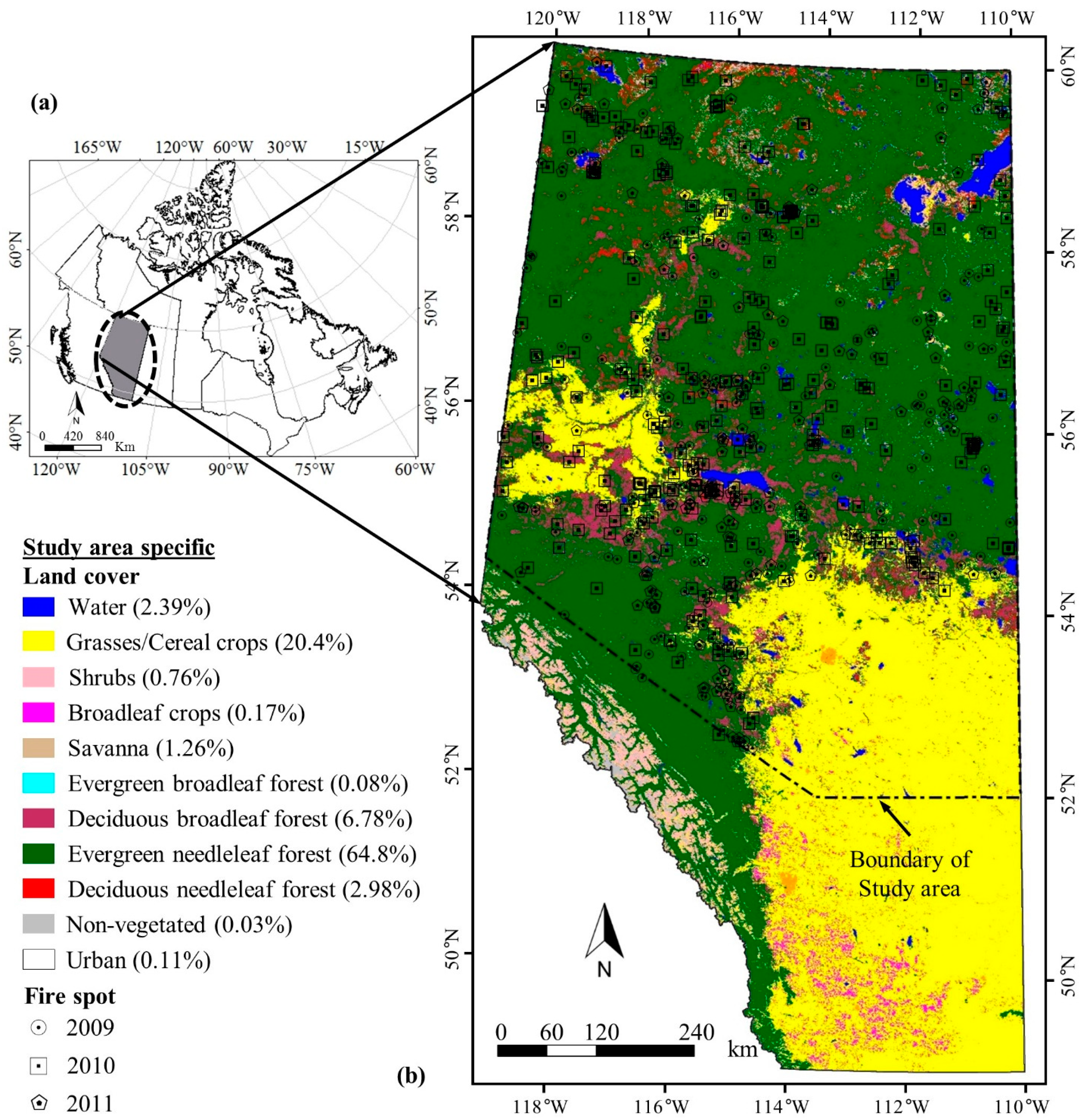
2.1. General Description of Study Area

The Canadian province of Alberta comprises six natural regions, which are categorized based on climate, topography, vegetation, soil and geological formations. Among these regions, the boreal forest alone occupies about 58% of the province [48] and often faces recurrent fire disturbances. For example, approximately 1560 fires occurred that burned about 196 thousand ha per annum on an average during the period 2003–2012 [49]. Here, we used the northern part of Alberta as our study area, which lies between 52–60°N latitude and 110–120°W longitude (Figure 1). The study area mainly covers eleven land cover types (see Figure 1), and among them, the four major forest land cover varieties (e.g., deciduous broadleaf forest, evergreen broadleaf forest, evergreen needleleaf forest, and deciduous needleleaf forest) occupy about 75% of the study area. The topography is highly variable and ranges between 162 to 3596 m above the mean sea level. The study area experiences cold winters and short warm summers and moderate annual precipitation that increases with elevation. The mean annual temperature and total precipitation vary from −3.6 to 1.1 °C, and 377–535 mm, respectively [48].

2.2. Data Requirements

We employed Terra MODIS-derived environmental variables for forecasting the forest fire danger conditions during 2009–2011 fire seasons. Those included: (i) 8-day composite of TS at 1 km spatial resolution, i.e., MOD11A2 v.005; (ii) 8-day composite of surface reflectance at 500 m spatial resolution, i.e., MOD9A1 v.005, which was subsequently used in calculating NMDI by use of near infrared (NIR) and shortwave infrared bands centered at 0.86 µm, 1.64 µm, and 2.13 µm, and NDVI by use of red and NIR spectral bands centered at 0.64 µm and 0.86 µm; and (iii) daily PW at 1 km spatial resolution, i.e., MOD05L2 v.051. The data were assimilated from 30 March–6 April to 22–29 September (i.e., DOY 89–96 to DOY 265–272) for TS, NMDI, and NDVI variables, and 30 March to 29 September (i.e., DOY 89 to DOY 272) for daily PW, respectively. In addition, we acquired an annual land cover map during 2008 derived from MODIS data at 500 m spatial resolution, i.e., MCD12Q1 v.005. In particular to the usage of remote sensing-based 8-day composite data had several issues, such as:
Figure 1. (a) Map of Canada showing the location of Alberta; and (b) spatial extent of the study area with dotted line shown over a MODIS-based annual land cover map of 2008 along with the fire occurrence spots available from Alberta ESRD during 2009–2011 fire seasons.
Remotesensing 07 02431 g001
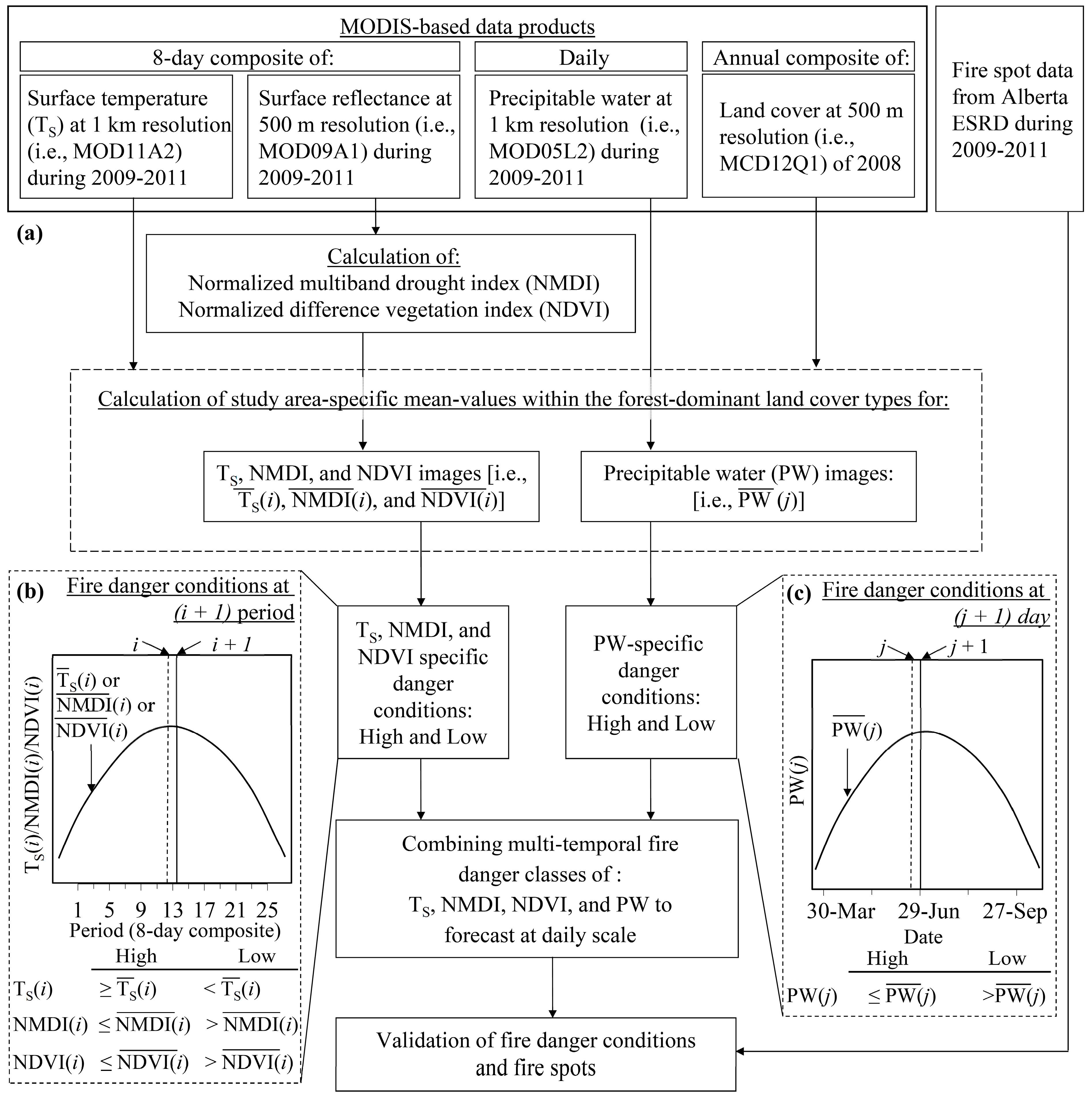
  • Though both TS and surface reflectance data (which were used to calculate NMDI, and NDVI) were available at daily temporal resolution, we employed their respective 8-day composite. This was because the computation of all these variables would be highly influenced by the atmospheric conditions, in particular the presence of cloud [50,51], which was critical in reducing the amount of cloud-contaminated pixels.
  • The 8-day composite of TS images were generated by averaging the TS images acquired under clear-sky conditions at approximately 10:30 am local time [52]. Thus, these values might not represent the daily variations and/or maximum temperature.
  • The 8-day composite of MODIS surface reflectance data used to calculate NMDI and NDVI was generated based on minimum-blue criterion, which coincided with the best clear-sky condition day during the composite of interest [53,54]. As such, two consecutive 8-day composite images might be apart in the range of 2 to 16 days. In addition, NMDI and NDVI variables were less dynamic in the temporal dimension, i.e., wetness/greenness condition of forest vegetation might not change over a short time period even though the vegetation would experience stresses [26].
Apart from the above-mentioned remote sensing data, we also used historical wildfire information available from Alberta Environment and Sustainable Resource Development (ESRD) during the 2009–2011 fire seasons. It consisted of several types of fire-related information, such as fire number, fire start date, fire location, and burned area. We considered those fire spots (i.e., the location of a fire started in a particular day) that eventually burned an area greater than or equal to 1 ha, as smaller fires might not be discernible by use of the spatial resolution of the commissioned environmental variables.

2.3. Implementation of a Gap-Filling Algorithm

Despite the usage of an 8-day composite of TS, NMDI, and NDVI images, there were still cloud-contaminated pixels in these images. In order to determine these data gaps, we employed MODIS quality assurance information for each variable of interest. Subsequently, we adopted the gap-filling algorithm to in-fill them described in [42], as follows:
X ( i ) = X ( i 1 ) + [ X ¯ ( i ) m × m X ¯ ( i 1 ) m × m ]
where, X(i) and X(i − 1) are the in-filled and non-contaminated values for the variables of TS, NMDI, and NDVI during i and i − 1 periods, respectively; X ¯ ( i ) m × m   a n d   X ¯ ( i 1 ) m × m are the average values of the variables of interest within m × m window size during i and i − 1 periods, respectively; and m × m is the window size in the range 3 × 3 to 15 × 15.
Prior to implementing any window size of interest, we always created artificial gaps over the good quality pixels and compared against the actual values. These good quality pixels were determined on the basis of the following characteristics: (i) for TS, when the average TS errors were reported ≤ 2 K; and (ii) for surface reflectance, we used the following set of criteria: cloud shadow (i.e., no), MOD35 cloud (i.e., clear), aerosol quality (i.e., climatology and low), internal cloud algorithm flag (i.e., no cloud), cirrus detected (i.e., none and small), and pixel adjacent to cloud (i.e., no). We only filled the gaps if the root mean square error (RMSE) was less than (i) 2 K for TS, which would be acceptable according to [55,56]; and (ii) 0.03 for both NMDI and NDVI, which would also be acceptable according to [53,57].
Note that we implemented the above-mentioned algorithm in an earlier study [42] in order to generate in-filled 8-day composite of TS, NMDI, and NDVI images during 2011 fire season. Thus, we filled the data gaps of these three variables of interest during the fire seasons of 2009 and 2010 in the scope of this study. However, we did not attempt to fill the data gaps in the daily PW image, because these gaps might be due to the presence of high moisture content in the atmosphere [58], which would potentially decrease the fire occurrences [59].
Upon employing the MODIS quality assurance information for each variable of interest, we found that the data gaps in the 8-day composite of TS, NMDI, and NDVI variables were in the range 0.52%–2.82%, 0.001%–0.0334%, and 0.00003%–0.0035%, respectively, on average during 2009–2011. Subsequently, we filled these gaps using both spatial (i.e., in the range 3 × 3 to 15 × 15 window sizes) and temporal (i.e., considering the images from i − 1 and i periods) dimensions for the variable of interest. We observed that the gaps were in-filled approximately (i) in the range 84.70% to 98.93% for TS images; and (ii) 100% for NMDI and NDVI images, during 2009–2011 period. The above results demonstrated that all the gap pixels could not be in-filled after implementing the gap-filling algorithm. The reasons behind the incapability to fill all the data-gaps were the lack of contamination-free pixels in both temporal (i.e., the pixel of interest was cloudy during i − 1 period) and spatial dimensions (i.e., none of the pixels were cloud-free within the window of interest) for the variable of interest [42,60].

2.4. Development of a Daily-Scale FFDFS

In this study, we developed a remote sensing-based FFDFS system at a daily scale using MODIS-derived variables, and its conceptual diagram is shown in Figure 2. The proposed system comprised of four steps. Firstly, we assimilated all four input variables (i.e., TS, NMDI, NDVI, and PW) within the four forest-dominant land cover types. Secondly, we computed the study area-specific average values for all input variables during the i period (i.e., T S ¯ ( i ) , NMDI ¯ ( i ) , NDVI ¯ ( i ) ) and j day (i.e., PW ¯ ( j ) ) . Thirdly, we calculated fire danger conditions (high or low; see Figure 2b,c) for each of the input variables during both i + 1 period and j + 1 day upon comparing the input variable-specific instantaneous values at a given pixel from i period and j day (i.e., TS(i), NMDI(i), NDVI(i), PW(j)) with their respective average values computed in the second step. We assumed that the fire danger condition for the specific variable of interest would be high if following condition would prevail. For example, T S ( i )     T S ¯ ( i ) : high temperature might favor fire; NMDI ( i )     NMDI ¯ ( i ) : low moisture in vegetation might support fire; NDVI ( i )     NDVI ¯ ( i ) : low vegetation greenness might support fire as it relates with other biophysical variables; and PW ( j )     PW ¯ ( j ) : low water vapor in the atmosphere might be associated with the flammability of both live and dead fuels. Finally, we stratified the individual input variable-specific danger conditions into five danger categories, such as: (i) extremely high: when all the four variables fell in the high danger class; (ii) very high: when at least three of the four variables fell in the high danger class; (iii) high: when at least two of the four variables fell in the high danger class; (iv) moderate: when at least one of the four variables fell in the high danger class; and (v) low: when all four variables fell in the low danger class. In integrating the individual variable-specific fire danger conditions in the framework of daily-scale FFDFS, we assumed that the impact of the 8-day composite of TS, NMDI, and NDVI variables would be constant over the following 8-day period.
After generating the daily fire danger maps, we evaluated them with the Alberta ESRD ground-based fire spots data during 2009–2011. In these cases, we overlaid the fire spots over the forecasted fire danger maps over a day of interest and computed the distribution of the fire danger categories over the fire spots. Finally, we determined the “% of each danger classes” over all of the fire spots during the entire study period. Note that we stratified all the multi-spatial input variables (i.e., TS, NMDI, NDVI, and PW) of the FFDFS so that the gridded pixels of each dataset matched. In this context, we resampled both the TS and PW images from 1 km to 500 m prior to integrating with the NMDI and NDVI images. Hence, our proposed FFDFS system would generate danger maps at a spatial resolution of 500 m.
Figure 2. (a) The conceptual diagram of daily-scale FFDFS; (b) fire danger conditions of 8-day scale TS, NMDI, and NDVI (based on Chowdhury and Hassan [42]); and (c) fire danger conditions of daily PW.
Remotesensing 07 02431 g002

3. Results and Discussion

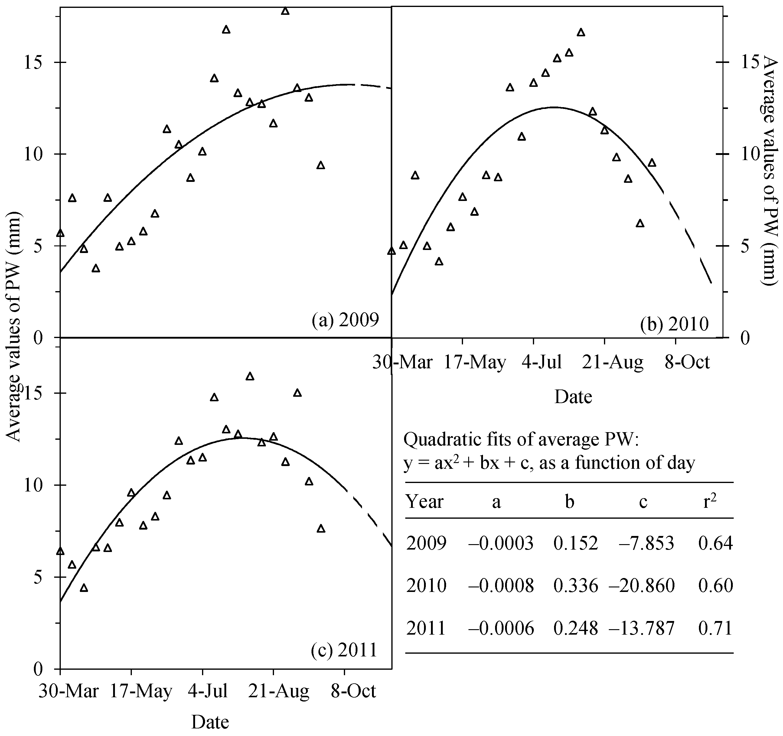
3.1. Evaluation of the Impact of Daily PW on the Fire Danger Condition

As we were incorporating the daily PW variable in the FFDFS framework for the first time, we opted to evaluate its individual impact on the fire danger conditions prior to integrating with other variables. As part of this process, we computed the study area-specific average values of PW ( PW ¯ ) in order to comprehend its seasonal trends. Then, we performed quadratic fits for the PW ¯ as a function of 8-day periods (see Figure 3). The r2-value for these curves were in the 0.60–0.71 range during the 2009–2011 period. Note that the generic shapes of these curves were similar to those illustrated in Figure 2c, which proved that our assumed pattern for the PW held quite nicely.
Figure 3. Study area-specific average values of PW (i.e., 8-day average) with day for the fire seasons of 2009–2011 (i.e., between 30 March to 29 September (i.e., DOY 89 and 272)).
Remotesensing 07 02431 g003
Upon getting the study area-specific daily ( PW ¯ ) during j day, we computed the daily PW-specific fire danger conditions (i.e., high and low) during j + 1 day, and compared them against the ground-based fire spots. It revealed that on average, 53.54% of fire spots fell under high danger category (i.e., PW(j) ≤ PW ¯ (j)) during the period of 2009–2011 (see Figure 4). These findings were found acceptable as the fire occurrences would not only depend on the PW but also other factors, e.g., temperature, precipitation, wind regimes, topography, fuel types, source of ignitions, etc. [8,26,61,62,63]. In addition, we observed that other input variables of the FFDFS (i.e., TS, NMDI, and NDVI) demonstrated similar results (i.e., 50.60%, 65.50%, and 61.95% of the fire spots fell under the “high danger” category for TS, NMDI, and NDVI respectively during 2009–2011). It could therefore be suggested that individual variables might not able to capture the fire danger conditions precisely.Furthermore, we analyzed the actual fire occurrence in the context of the study area-specific average and standard deviations associated with PW (see Figure 4) and observed two major issues. Firstly, we did not find whether relatively lower PW (i.e., less than “average-1 standard deviation”) was related to more fire occurrences. In fact, similar situations were also observed for the variables TS, NMDI, and TVWI over boreal forested regions of Alberta in [41]. Also, Bartsch et al. [64] noticed that more dryness did not always favour fire occurrences while investigating soil moisture anomalies as a fire danger indicator over Siberia. Secondly, we found that approximately 70.44% of the fires fell within “average ± 1 standard deviation” and similar results were also reported in other studies, e.g.,:
  • Clabo and Bunkers [65] found that most of the fires occurred in South Dakota when the PW in the 800–700 mb layer (i.e., ~1.8–2.7 km above the ground surface) was below or around the monthly PW ¯ -levels;
  • Sitnov and Mokhov [47] observed the daily PWs were highly anomalous (i.e., water vapor content was low compared to that of the ten years average-values) during 23 July to 18 August 2010 over European Russia when more than 60% of the fires took place; and
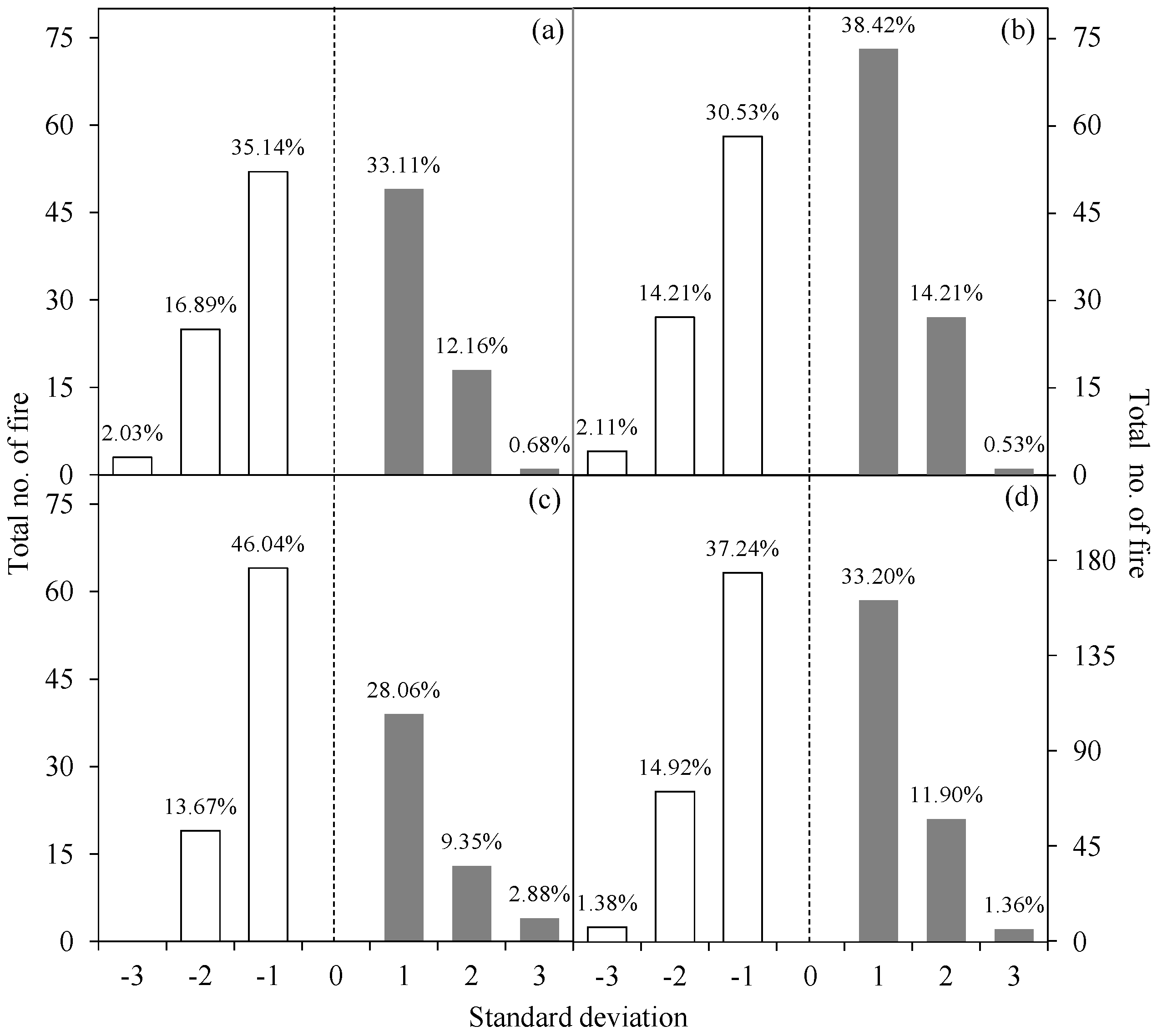
  • Akther and Hassan [41] reported that most of the fire occurrences were found within the “average ± 1 standard deviation” for the variables TS, NMDI, and TVWI over boreal forested regions of Alberta.
Figure 4. Frequency distribution of the fires with respect to the PW variable and its corresponding study area average values during the j day when actual fires occurred in the following j + 1 day on the basis of the “study area-specific average ±3 standard deviation” values and percentage of fire spots during (a) 2009, (b) 2010, (c) 2011, and (d) 2009–2011.
Remotesensing 07 02431 g004
Additionally, the daily PW variable was based on total column of water vapor amounts in the atmosphere and usually found to be very sensitive to boundary-layer water vapor [66]. Also, relationships between water vapor at different boundary layers and fire occurrences were reported in the literature; (i) Brotak [67] found that low moisture at the 850 mb layer was highly associated with severe fires in the eastern United States (i.e., 93% of the all fire occurrences); and (ii) Price [68] showed that PW at above 300 mb and the 300–500 mb layer was linked to lightning activity, which would be considered one of the major source of fire ignition. Note that in Canada alone, lightning-caused fire burned more than 1.6 million ha of forested land annually on average [69]. As a result, it would be worthwhile to investigate the water vapor regimes at different boundary layers and their relationship with fire occurrences. In such cases, one of the viable options would be the use of radiosonde data [67,68].

3.2. Evaluation of Daily-Scale FFDFS System

Once the variable-specific (i.e., TS, NMDI, NDVI, and PW) fire danger conditions (i.e., either high or low) were generated, we combined all the variables of interest to forecast the fire danger conditions at the daily scale. The combined fire danger conditions demonstrated excellent results, i.e., on average 95.51% of the fires fell under “extremely high” to “moderate” danger classes during the 2009–2011 period (Table 1). In addition, we also observed very good results using the combined variables of TS, NMDI, and NDVI at the 8-day scale while comparing with the Alberta ESRD fire data from 2009–2011 (Table 2). They show that on average, 90.94% of the fires fell in “very high” to “moderate” danger classes. It was clearly evident that the daily-scale FFDFS performed better than the 8-day scale FFDFS, i.e., improvement over 4.5% during the period of 2009–2011. However, the major enhancement of the FFDFS system was the capability to forecast fire danger conditions at the daily scale, which would be a prerequisite from an operational perspective.
Table 1. Percentage of data under each fire danger category using the combined variable of TS, NMDI, NDVI, and PW in comparison with the fire spot.
YearNo. of Variables Fulfilling the Danger ConditionFire Danger Categories% of DataCumulative % of Data
AllExtremely High8.958.95
At least 3Very High28.3637.31
2009At least 2High36.5773.88
At least 1Moderate20.9094.78
NoneLow5.22100.00
AllExtremely High14.8814.88
At least 3Very High30.9545.83
2010At least 2High30.3676.19
At least 1Moderate19.6495.83
NoneLow4.17100.00
AllExtremely High15.4415.44
At least 3Very High36.5952.03
2011At least 2High30.0882.11
At least 1Moderate13.8295.93
NoneLow4.07100.00
AllExtremely High13.0813.08
At least 3Very High31.9745.05
2009–2011At least 2High32.3477.39
At least 1Moderate18.1295.51
NoneLow4.49100.00
Table 2. Percentage of data under each fire danger category using the combined variable of TS, NMDI, and NDVI in comparison with the fire spot.
YearNo. of Variables Fulfilling the Danger ConditionFire Danger Categories% of DataCumulative % of Data
2009AllVery High22.9222.92
At least 2High31.9454.86
At least 1Moderate34.0388.89
NoneLow11.11100.00
2010AllVery High30.7730.77
At least 2High35.1665.93
At least 1Moderate24.7390.66
NoneLow9.34100.00
2011AllVery High32.8432.84
At least 2High31.3464.18
At least 1Moderate29.1093.28
NoneLow6.72100.00
2009-2011AllVery High28.8428.84
At least 2High32.8161.65
At least 1Moderate29.2990.94
NoneLow9.06100.00
Figure 5 shows the combined fire danger map at 500 m spatial resolution for 13 June 2009 (i.e., DOY 164) while the input variables were acquired during the immediate preceding day (i.e., 12 June 2009; DOY 163) for PW, and period (i.e., 2–9 June 2009; DOY 153–160) for TS, NMDI, and NDVI. The fire danger map shown in Figure 5 revealed that approximately 91.50% of the pixels fell into the “extremely high” to “moderate” danger categories. In addition, we observed that the actual fires that started in 13 June 2009 (i.e., 23 fires that burned more than 36,000 ha) and their specific danger conditions demonstrated that 95.24% of fire fell under “extremely high” to “moderate” danger classes (sample fire spots along with the danger conditions are shown in Figure 5b). Note that our observed agreements were similar to the 8-day scale forecasting, such as 91.6 and 98.19% of fires falling under “very high” to ”moderate” danger categories in [41,42] respectively.
Despite the excellent performance of the FFDFS, we observed that a small percentage of the fire spots (i.e., 4.49%) fell in the low danger category, which could be improved upon by considering other fire-related variables. Those might include the incorporation of (i) spatially dynamic but temporally static (e.g., topographic parameters such as slope, elevation, and aspect, proximity to road networks, and proximity to urban areas) [62] and spatially static but temporally dynamic (e.g., the effect of long weekends would attract more people to camp in forests) variables; (ii) other meteorological variables, such as incident solar radiation, amount and duration of precipitation, wind regimes; (iii) lightning as a source of ignition; (iv) vegetation phenology as it might play an important role in defining water stress and thus fire occurrence [22]; and (v) relatively higher spatial resolution (e.g., 250 m) for the input variables in delineating the landscape in more detail [70]. Among these, wind regimes are commonly used in most of the operational systems; however, we were unable to incorporate such a variable in our proposed FFDFS as remote sensing-based estimates of wind regimes would be extremely difficult.
Figure 5. (a) Fire danger map for 13 June 2009, forecasted by combining the TS, NMDI, NDVI, and PW variables exploited during the immediate preceding day i.e., 12 June 2009; and actual fire occurrences during 13 June 2009 (i.e., DOY 164); (b) fire danger classes with actual fire spot.
Remotesensing 07 02431 g005

4. Concluding Remarks

In the course of this study, we developed a simple but unique fully remote sensing-based framework for forecasting daily forest fire danger conditions at 500 m spatial resolution. This proposed system consisted of three steps: (i) processing of the input variables (i.e., TS, NMDI, NDVI, and PW) of the FFDFS system, and computation of their respective study-area specific average values; (ii) determination of variable-specific fire danger conditions (either high or low); and (iii) stratification of all the four variable-specific fire danger conditions into five fire danger categories (i.e., extremely high, very high, high, moderate, and low). The proposed daily-scale FFDFS system revealed that 94.78%–95.93% of the fires fell under “extremely high” to “moderate” danger classes during the 2009–2011 period. We believe that the proposed system would be useful in supplementing the currently operational meteorological-based forecasting systems, in particular for remote areas of the landscape and in between two weather stations. Also, the proposed system could potentially be adopted in other jurisdictions and/or globally; however, we strongly recommend that it should be thoroughly evaluated prior to its implementation.

Acknowledgments

The study was funded by an NSERC Discovery Grant to Hassan. We would like to acknowledge the Queen Elizabeth II scholarship given to E. Chowdhury. We are indebted to NASA for providing the MODIS data free of cost and Alberta Environment and Sustainable Resource Development for making fire-related data freely available. In addition, we would like to acknowledge the anonymous reviewers for commenting on our paper.

Author Contributions

Ehsan H. Chowdhury was responsible for data acquisition, pre-processing, and development of the methods under the direction of Quazi K. Hassan. Both authors were significantly involved in writing this article.

Conflicts of Interest

The authors declare no conflict of interest.

References and Notes

  1. Natural Resources Canada (NRCAN). Fire. Available online: http://www.nrcan.gc.ca/forests/fire/13143 (accessed on 29 November 2014).
  2. Montealegre, A.L.; Lamelas, M.T.; Tanase, M.A.; de la Riva, J. Forest fire severity assessment using ALS data in a Mediterranean environment. Remote Sens. 2014, 6, 4240–4265. [Google Scholar] [CrossRef]
  3. Ruokolainen, L.; Salo, K. The effect of fire intensity on vegetation succession on a sub-xeric health during ten years after wildfire. Ann. Bot. Fennici 2009, 46, 30–42. [Google Scholar] [CrossRef]
  4. Chu, T.; Guo, X. Remote sensing techniques in monitoring post-fire effects and patterns of forest recovery in Boreal forest regions: A review. Remote Sens. 2014, 6, 470–520. [Google Scholar] [CrossRef]
  5. Souza, C.M., Jr.; Siqueira, J.V.; Sales, M.H.; Fonseca, A.V.; Ribeiro, J.G.; Numata, I.; Cochrane, M.A.; Barber, C.P.; Roberts, D.A.; Barlow, J. Ten-year Landsat classification of deforestation and forest degradation in the Brazilian Amazon. Remote Sens. 2013, 5, 5493–5513. [Google Scholar] [CrossRef]
  6. Flannigan, M.; Stocks, B.; Turetsky, M.; Wotton, M. Impacts of climate change on fire activity and fire management in the circumboreal forest. Glob. Change Biol. 2009, 15, 549–560. [Google Scholar] [CrossRef]
  7. Vadrevu, K.P.; Csiszar, I.; Ellicott, E.; Giglip, L.; Badarinath, K.V.S.; Vermote, E.; Justice, C. Hotspot analysis of vegetation fires and intensity in the Indian region. IEEE J. Sel. Top. Appl. Earth Obs. Remote Sens. 2013, 6, 224–238. [Google Scholar] [CrossRef]
  8. Van Wagner, C.E. Development and Structure of the Canadian Forest Fire Weather Index; Government of Canada: Ottawa, ON, Canada, 1987; pp. 1–37. [Google Scholar]
  9. Taylor, S.W. Considerations of applying the Canadian Forest Fire Danger Rating System in Argentina. Unpublished report. Canadian Forest Service, Pacific Forestry Centre: Victoria, BC, Canada, 2001; 1–25. [Google Scholar]
  10. Alexander, M.E.; Cole, F.V. Rating fire danger in Alaska ecosystems: CFFDRS provides an invaluable guide to systematically evaluating burning conditions. Fireline 2001, 12, 2–3. [Google Scholar]
  11. De Groot, W.J.; Field, R.D.; Brady, M.A.; Roswintiarti, O.; Mohamad, M. Development of the Indonesian and Malaysian Fire Danger Rating Systems. Mitig. Adapt. Strat. Glob. Change 2007, 12, 165–180. [Google Scholar] [CrossRef]
  12. Lee, B.S.; Alexander, M.E.; Hawkes, B.C.; Lynham, T.J.; Stocks, B.J.; Englefield, P. Information systems in support of wildland fire management decision making in Canada. Comput. Electron. Agric. 2002, 37, 185–198. [Google Scholar] [CrossRef]
  13. Alexander, M.E.; Fogarty, L.G. A Pocket Card for Predicting Fire Behavior in Grasslands under Severe Burning Conditions; Fire Technology Transfer Note 25; Natural Resources Canada, Canadian Forest Service: Ottawa, ON, Canada, 2002; pp. 1–8. [Google Scholar]
  14. San-Miguel-Ayanz, J.; Barbosa, P.; Liberta, G.; Schmuck, G.; Schulte, E.; Bucella, P. The European forest fire information system: A European strategy towards forest fire management. In Proceedings of the 3rd International Wildland Fire Conference, Sydney, Australia, 3–6 October 2003.
  15. Viegas, D.X.; Bovio, G.; Ferreira, A.; Nosenzo, A.; Sol, B. Comparative study of various methods of fire danger evaluation in southern Europe. Int. J. Wildland Fire 1999, 9, 235–246. [Google Scholar] [CrossRef]
  16. Granstrom, A.; Schimmel, J. Assessment of the Canadian Forest Fire Danger System for Swedish Fuel Conditions (in Swedish); Rescue Services Agency: Stockholm, Sweden, 1998; pp. 1–34. [Google Scholar]
  17. Chilès, J.-P.; Delfiner, P. Geostatistics Modeling Spatial Uncertainty, 2nd ed.; John Wiley & Sons Inc.: Hoboken, NJ, USA, 2012; pp. 1–699. [Google Scholar]
  18. Molders, N. Suitability of the Weather Research and Forecasting (WRF) Model to Predict the June 2005 Fire Weather for Interior Alaska. Wea. Forecast. 2008, 23, 953–973. [Google Scholar] [CrossRef]
  19. Peterson, D.; Hyer, E.; Wang, J. A short-term predictor of satellite-observed fire activity in the North American boreal forest: Toward improving the prediction of smoke emissions. Atmos. Environ. 2013, 71, 304–310. [Google Scholar] [CrossRef]
  20. Leblon, B.; Bourgeau-Chavez, L.; San-Miguel-Ayanz, J. Sustainable development-authoritative and leading edge content for environmental management. In Use of Remote Sensing in Wildfire Management; Curkovic, S., Ed.; InTech: Croatia, Yugoslavia, 2012; pp. 55–81. [Google Scholar]
  21. Ceccato, P.; Flasse, S.; Tarantola, S.; Jacquemoud, S.; Grégoire, J.-M. Detecting vegetation leaf water content using reflectance in the optical domain. Remote Sens. Environ. 2001, 77, 22–33. [Google Scholar] [CrossRef]
  22. Bajocco, S.; Rosati, L.; Ricotta, C. Knowing fire incidence through fuel phenology: A remotely sensed approach. Ecol. Model. 2010, 221, 59–66. [Google Scholar] [CrossRef]
  23. Leblon, B.; García, P.A.F.; Oldford, S.; Maclean, D.A.; Flannigan, M. Using cumulative NOAA-AVHRR spectral indices for estimating fire danger codes in northern boreal forests. Int. J. Appl. Earth Obs. Geoinf. 2007, 9, 335–342. [Google Scholar] [CrossRef]
  24. Oldford, S.; Leblon, B.; Maclean, D.; Flannigan, M. Predicting slow‐drying fire weather index fuel moisture codes with NOAA‐AVHRR images in Canada’s northern boreal forests. Int. J. Remote Sens. 2006, 27, 3881–3902. [Google Scholar] [CrossRef]
  25. Nieto, H.; Aguadoa, I.; Chuvieco, E.; Sandholt, I. Dead fuel moisture estimation with MSG-SEVIRI data. Retrieval of meteorological data for the calculation of equilibrium moisture content. Agric. For. Meteorol. 2010, 150, 861–870. [Google Scholar] [CrossRef]
  26. Leblon, B.; Alexander, M.; Chen, J.; White, S. Monitoring fire danger of northern boreal forests with NOAA-AVHRR NDVI images. Int. J. Remote Sens. 2001, 22, 2839–2846. [Google Scholar] [CrossRef]
  27. Bisquert, M.M.; Sanchez, J.M.; Caselles, V. Fire danger estimation from MODIS Enhanced Vegetation Index data: Application to Galicia region (North-west Spain). Int. J. Wildland Fire 2011, 20, 465–473. [Google Scholar] [CrossRef]
  28. Bisquert, M.; Sanchez, J.M.; Caselles, V. Modeling fire danger in Glacia and Asturias (Spain) from MODIS images. Remote Sens. 2014, 6, 540–554. [Google Scholar] [CrossRef]
  29. Schneider, P.; Roberts, D.A.; Kyriakidis, P.C. A VARI-based relative greenness from MODIS data for computing the fire potential index. Remote Sens. Environ. 2008, 112, 1151–1167. [Google Scholar] [CrossRef]
  30. Rahimzadeh-Bajgiran, P.; Omasa, K.; Shimizu, Y. Comparative evaluation of the vegetation dryness index (VDI), the temperature vegetation dryness index (TVDI), and the improved TVDI (iTVDI) for water stress detection in semi-arid regions of Iran. ISPRS J. Photogram. Remote Sens. 2012, 68, 1–12. [Google Scholar] [CrossRef]
  31. Aguado, I.; Chuvieco, E.; Martin, P.; Salas, J. Assessment of forest fire danger conditions in southern Spain from NOAA images and meteorological indices. Int. J. Remote Sens. 2003, 24, 1653–1668. [Google Scholar] [CrossRef]
  32. Mildrexler, D.J.; Zhao, M.; Heinsch, F.A.; Running, S.W. A new satellite-based methodology for continental-scale disturbance detection. Ecol. Appl. 2007, 17, 235–250. [Google Scholar] [CrossRef] [PubMed]
  33. Wang, L.; Qu, J.J.; Hao, X. Forest fire detection using normalized multi-band drought index (NMDI) with satellite measurements. Agric. For. Meteorol. 2008, 148, 1767–1776. [Google Scholar] [CrossRef]
  34. Stow, D.; Niphadkar, M.; Kaiser, J. MODIS-derived visible atmospherically resistant index for monitoring chaparral moisture content. Int. J. Remote Sens. 2005, 26, 3867–3873. [Google Scholar] [CrossRef]
  35. Peterson, S.H.; Roberts, D.A.; Dennison, P.E. Mapping live fuel moisture with MODIS data: A multiple regression approach. Remote Sens. Environ. 2008, 112, 4272–4284. [Google Scholar] [CrossRef]
  36. Sow, M.; Mbow, C.; Hély, C.; Fensholt, R.; Sambou, B. Estimation of herbaceous fuel moisture content using vegetation indices and land surface temperature from MODIS data. Remote Sens. 2013, 5, 2617–2638. [Google Scholar] [CrossRef]
  37. Chowdhury, E.H.; Hassan, Q.K. Operational perspective of remote sensing-based forest fire danger forecasting systems. ISPRS J. Photogram. Remote Sens. 2014. [Google Scholar] [CrossRef]
  38. Vidal, A.; Devaux-Ros, C. Evaluating forest fire hazard with a Landsat TM derived water stress index. Agric. For. Meteorol. 1995, 77, 207–224. [Google Scholar] [CrossRef]
  39. Guangmeng, G.; Mei, Z. Using MODIS land surface temperature to evaluate forest fire risk of northeast China. IEEE Geosci. Remote Sens. Lett. 2004, 1, 98–100. [Google Scholar] [CrossRef]
  40. Oldford, S.; Leblon, B.; Gallant, L. Mapping pre-fire forest conditions with NOAA-AVHRR images in northern boreal forests. Geocarto Int. 2003, 18, 21–32. [Google Scholar] [CrossRef]
  41. Akther, M.S.; Hassan, Q.K. Remote sensing-based assessment of fire danger conditions over boreal forest. IEEE J. Sel. Top. Appl. Earth Obs. Remote Sens. 2011, 4, 992–999. [Google Scholar] [CrossRef]
  42. Chowdhury, E.H.; Hassan, Q.K. Use of remote sensing-derived variables in developing a forest fire danger forecasting system. Nat. Hazards 2013, 67, 321–334. [Google Scholar] [CrossRef]
  43. Burgan, R.E. 1988 Revisions to the 1978 National Fire-danger Rating System; U.S. Department of Agriculture, Forest Service: Asheville, NC, USA, 1988; pp. 1–39. [Google Scholar]
  44. McArthur, A.G. Fire Behavior in Eucalypt Forests; Australia Forestry and Timber Bureau: Canberra, Australia, 1967; pp. 1–36. [Google Scholar]
  45. Nesterov, V.G. Forest Fire Danger and Methods of Its Determination; USSR State Industry Press: Goslesbumizdat, Moscow, Russia, 1949; pp. 1–76. [Google Scholar]
  46. Han, K.; Viay, A.A.; Anctil, F. High-resolution forest fire weather index computations using satellite remote sensing. Can. J. Forest Res. 2003, 33, 1134–1143. [Google Scholar] [CrossRef]
  47. Sitnov, S.A.; Mokhov, I.I. Water-vapor content in the atmosphere over European Russia during the summer 2010 fires. Atmos. Ocean. Phys. 2013, 49, 380–394. [Google Scholar] [CrossRef]
  48. Downing, D.J.; Pettapiece, W.W. Natural Regions and Subregions of Alberta; Natural regions committee, Government of Alberta: Edmonton, AB, Canada, 2006; pp. 1–254. [Google Scholar]
  49. Environment and Sustainable Resource Development (ESRD). 10-Year Wildfire Statistics. Available online: http://www.srd.alberta.ca/Wildfire/WildfireStatus/HistoricalWildfireInformation/10-YearStatisticalSummary.aspx (accessed on 23 June 2014).
  50. Wan, Z. MODIS Land-Surface Temperature Algorithm Theoretical Basis Document, Version 3.3; University of California: Santa Barbara, CA, USA, 1999; pp. 1–77. Available online: http://modis.gsfc.nasa.gov/data/atbd/atbd_mod11.pdf (accessed on 15 January 2011).
  51. Vermote, E.F.; Vermeulen, A. MODIS Algorithm Theoretical Basis Document, Atmospheric Correction Algorithm: Spectral Reflectances (MOD09), Version 4.0; University of Maryland: College Park, MD, USA, 1999; pp. 1–107. Available online: http://modis.gsfc.nasa.gov/data/atbd/atbd_mod08.pdf (accessed on 15 January 2011).
  52. Wan, Z. MODIS Land Surface Temperature Products User`s Guide, Collection 5; University of California: Santa Barbara, CA, USA, 2006; pp. 1–30. Available online: http://www.icess.ucsb.edu/modis/LstUsrGuide/MODIS_LST_products_Users_guide_C5.pdf (accessed on 10 December 2011).
  53. Vermote, E.F.; Kotchenova, S.Y.; Ray, J.P. MODIS Surface Reflectance User’s Guide, Version 1.3; University of Maryland: College Park, MD, USA, 2011; pp. 1–40. Available online: http://modis-sr.ltdri.org/products/MOD09_UserGuide_v1_3.pdf (accessed on 15 January 2011).
  54. Descloitres, J; Vermote, E. Operational retrieval of the spectral surface reflectance and vegetation index at global scale from SeaWiFS data. In Proceedings of the International Conference and Workshops on Ocean Color, Land Surfaces, Radiation and Clouds, Aerosols, ALPS.99: The contribution of POLDER and new generation spaceborne sensors to global change studies, Meribel, France, 18–22 January 1999.
  55. Wan, Z. New refinements and validation of the collection-6 MODIS land-surface temperature/emissivity product. Remote Sens. Environ. 2014, 140, 36–45. [Google Scholar] [CrossRef]
  56. Oyoshi, K.; Akatsuka, S.; Takeuchi, W.; Sobue, S. Hourly LST monitoring with the Japanese geostationary satellite MTSAT-1R over the Asia-Pacific region. Asian J. Geoinform. 2014, 14, 1–13. [Google Scholar]
  57. Gao, X.; Huete, A.R.; Didan, K. Multisensor comparisons and validation of MODIS vegetation indices at the semiarid Jordana experimental range. IEEE Trans. Geosci. Remote Sens. 2003, 41, 2368–2381. [Google Scholar] [CrossRef]
  58. Kaufman, Y.K.; Gao, B-O. Remote sensing of water vapor in the Near IR from EOS/MODIS. IEEE Trans. Geosci. Remote Sens. 1992, 30, 871–884. [Google Scholar] [CrossRef]
  59. Haines, D.A. A lower atmospheric severity index for wildland fires. Natl. Wea. Dig. 1988, 13, 23–27. [Google Scholar]
  60. Kang, S.; Running, S.W.; Zhao, M.; Kimball, J.S.; Glassy, J. Improving continuity of MODIS terrestrial photosynthesis products using an interpolation scheme for cloudy pixels. Int. J. Remote Sens. 2005, 26, 1659–1676. [Google Scholar] [CrossRef]
  61. Lecina-Diaz, J.; Alvarez, A.; Retana, J. Extreme fire severity patterns in topographic, convective and wind-driven historical wildfires of Mediterranean pine forests. PLoS One 2014, 9, e85127. [Google Scholar] [CrossRef] [PubMed] [Green Version]
  62. Adab, H.; Kanniah, K.D.; Solaimani, K. Modeling forest fire risk in the northeast of Iran using remote sensing and GIS techniques. Nat. Hazards 2013, 65, 1723–1743. [Google Scholar] [CrossRef]
  63. Ardakani, A.S.; Zoej, M.J.V.; Mohammadzadeh, A.; Mansourian, A. Spatial and temporal analysis of fires detected by MODIS data in northern Iran from 2001 to 2008. IEEE J. Sel. Top. Appl. Earth Obs. Remote Sens. 2011, 4, 216–225. [Google Scholar] [CrossRef]
  64. Bartsch, A.; Balzter, H.; George, C. The influence of regional surface soil moisture anomalies on forest fires in Siberia observed from satellites. Environ. Res. Lett. 2009, 4, 045021. [Google Scholar] [CrossRef]
  65. Clabo, D.R.; Bunkers, M.J. Using variable column precipitable water as a predictor for large fire potential. In Weather and Climate Impacts, Proceedings of the Ninth Symposium on Fire and Forest Meteorology, Palm Springs, CA, USA, 20 October 2011; American Meteorological Society: Boston, MA, USA.
  66. Gao, B.-C.; Kaufman, Y.J. Algorithm Technical Background Document, The MODIS Near-IR Water Vapor Algorithm, Product ID: MOD05—Total Precipitable Water. Available online: http://modis-atmos.gsfc.nasa.gov/_docs/atbd_mod03.pdf (accessed on 10 January 2014).
  67. Brotak, E.A. An investigation of the synoptic situations associated with major wildland fire. J. Appl. Meteorol. 1977, 16, 867–870. [Google Scholar] [CrossRef]
  68. Price, C. Evidence for a link between global lightning activity and upper tropospheric water vapour. Nature 2000, 406, 290–293. [Google Scholar] [CrossRef] [PubMed]
  69. Stocks, B.J.; Mason, J.A.; Todd, J.B.; Bosch, E.M.; Wotton, B.M.; Amiro, B.D.; Flannigan, M.D.; Hirsch, K.G.; Logan, K.A.; Martell, D.L.; et al. Large forest fires in Canada, 1959–1997. J. Geophys. Res. 2003, 108, 8149. [Google Scholar] [CrossRef]
  70. Wing, M.G.; Burnett, J.D.; Sessions, J. Remote sensing and unmanned aerial system technology for monitoring and quantifying forest fire impacts. Int. J. Remote Sens. Appl. 2014, 4, 18–35. [Google Scholar] [CrossRef]

