Article

Using Ridge Regression Models to Estimate Grain Yield from Field Spectral Data in Bread Wheat (Triticum Aestivum L.) Grown under Three Water Regimes

by
Javier Hernandez
1,*,
Gustavo A. Lobos
2,†,
Iván Matus
3,†,
Alejandro Del Pozo
2,†,
Paola Silva
1,† and
Mauricio Galleguillos
4,*
1
Department of Agricultural Production, Faculty of Agronomics Sciences, University of Chile, Santiago, Casilla 1004, Chile
2
Plant Breeding and Phenomic Center, Faculty of Agricultural Sciences, University of Talca, Talca, Casilla 747–721, Chile
3
Research Regional Center-Quilamapu, Agricultural Research Institute, Chillán, Casilla 426, Chile
4
Department of Environmental Sciences, Faculty of Agronomic Sciences, University of Chile, Santa Rosa 11315, La Pintana, Santiago, Chile
*
Authors to whom correspondence should be addressed.
These authors contributed equally to this work.
Remote Sens. 2015, 7(2), 2109-2126; https://doi.org/10.3390/rs70202109
Submission received: 23 July 2014 / Accepted: 27 January 2015 / Published: 16 February 2015

Abstract

:
Plant breeding based on grain yield (GY) is an expensive and time-consuming method, so new indirect estimation techniques to evaluate the performance of crops represent an alternative method to improve grain yield. The present study evaluated the ability of canopy reflectance spectroscopy at the range from 350 to 2500 nm to predict GY in a large panel (368 genotypes) of wheat (Triticum aestivum L.) through multivariate ridge regression models. Plants were treated under three water regimes in the Mediterranean conditions of central Chile: severe water stress (SWS, rain fed), mild water stress (MWS; one irrigation event around booting) and full irrigation (FI) with mean GYs of 1655, 4739, and 7967 kg∙ha−1, respectively. Models developed from reflectance data during anthesis and grain filling under all water regimes explained between 77% and 91% of the GY variability, with the highest values in SWS condition. When individual models were used to predict yield in the rest of the trials assessed, models fitted during anthesis under MWS performed best. Combined models using data from different water regimes and each phenological stage were used to predict grain yield, and the coefficients of determination (R2) increased to 89.9% and 92.0% for anthesis and grain filling, respectively. The model generated during anthesis in MWS was the best at predicting yields when it was applied to other conditions. Comparisons against conventional reflectance indices were made, showing lower predictive abilities. It was concluded that a Ridge Regression Model using a data set based on spectral reflectance at anthesis or grain filling represents an effective method to predict grain yield in genotypes under different water regimes.

Graphical Abstract

1. Introduction

Breeding programs must evaluate different agronomic and physiological traits in a large number (thousands) of genotypes that result from various crossings [1,2,3]. One of the traits is grain yield (GY), which has low heritability and a high genotype by environment interaction. Yield production is particularly sensitive to the meteorological conditions that occur from anthesis to grain filling. Therefore, evaluation of genotypes yields in different environments and growing seasons is required [1,4]. Breeding based on GY has been restricted to Mediterranean dryland environments because the most limiting factor of yield is drought stress [5,6,7]. Thus, creating methods that are able to indirectly estimate the GY of different genotypes in intermediate stages of development could reduce costs and the time needed to measure them [8,9].
During wheat growth, the leaves, canopy and spikes can absorb, reflect, or transmit energy reaching the surface due to interaction of incident radiation with the plant structure and photosynthetic elements [10,11]. By determining the spectral signature of canopy and leaf reflectance with a spectroradiometer, it is possible to indirectly measure agronomic and physiological traits [9,12] such as chlorophyll content [13,14], aerial biomass [15], plant water content [16], or grain yield [17,18]. Indices based on reflectance at different wavelengths, known as spectral reflectance indices (SRIs), have been used for this purpose [17,19,20,21]. Several of these indices have also been positively correlated (using logarithmic or linear models) with crop dry matter (DM), leaf area index (LAI), green area index (GAI), and potential photosynthetic capacity [5,17,20]. However, these indices only use a limited portion of the spectral information by reducing, simplifying, or not considering the abundant information it contains [22,23]. Also, optimal wavelengths for estimating traits, such as GY, can vary in accordance with the phenological stage and environmental conditions [18,24].
Because remote sensing sensors usually intercept more wavelengths than those used by the indices, it has been proposed that all information from hyperspectral sensors be used through linear regression techniques that use multivariate inputs. [23,24,25]. One of the approaches is a linear regression model based on least squares; however, this technique performs poorly when input variables are collinear or exceed the number of training cases [26,27]. This is why regression techniques based on penalizing regression parameters and linear combination from the predictor variables are more appropriate for spectral assessment [26,28]. According to Ferrio et al. [25], this type of approach should be proven empirically in the field to understand the indirect relationship between wavelengths and GY because it can vary depending on the environmental conditions and location. In durum wheat [25] and maize [24], GY prediction has been evaluated by multivariate techniques using partial least square regression (PLRS). This technique breaks down all the variability of spectral information into a few factors that determine GY and leads to correct results. Other models use the whole information generated by spectral measurements, such as ridge regression, which was introduced by Tikhonov [29] and generalized by Hoerl and Kennard [30]. This type of multivariate linear regression includes a contraction of the multivariate model regression coefficients and reduces them to the same degree [27].
In this context, new methodologies that manage a wide range of information from canopy reflectance should be studied to identify their potential use in estimating GY. The main objective of the present study was to evaluate the ability of canopy reflectance to predict GY in a wide range of bread wheat genotypes through a multivariate regression technique. In addition, the model was evaluated under three water regimes and two phenological stages to assess its ability to predict and operate under conditions different to those from which it was generated. Comparisons against conventional spectral indices are also presented.

2. Experimental Section

2.1. Plant Material and Experimental Sites

A set of 368 advanced spring wheat (Triticum aestivum) lines from three breeding programs, INIA-Chile, INIA-Uruguay and CIMMYT, were evaluated in two Mediterranean environments in central Chile during the 2011-2012 season. The sites were Cauquenes (35°58′S, 72°17′W; 177 m.a.s.l.) under rainfed or severe water stress (SWS) conditions and Santa Rosa (36°32′S, 71°55′W; 217 m.a.s.l.) under two water regimes: mild water stress (MWS) and full irrigation (FI). At Cauquenes the average annual temperature is 14.7 °C, the minimum average is 4.7 °C (July) and the maximum average is 27 °C (January) [31]; the annual precipitation was 410 mm in 2011. The soil was granitic with a sandy clay loam texture, classified as Ultic Palexeralfs [31]. Santa Rosa corresponds to a high yielding area; the average annual temperature in this region is 13.0 °C, the minimum average is 3.0 °C (July) and the maximum average is 28.6 °C (January) [32]; the annual precipitation was 736 mm in 2011. The soil is formed from volcanic ash of silt loam texture, classified as Melanoxerands.
Each experimental unit consisted of five rows, 2 m long with a separation of 0.2 m between rows, and a 20 gr∙m−2 seed rate. An alpha lattice experimental design with one replicate was used, with the exception of the FI environment, which had two replicates. Crops were sown on 7 September in Cauquenes and 31 August in Santa Rosa. Plot fertilization was as follows: 260 kg∙ha−1 ammonium phosphate (46% P2O5 and 18% N), 90 kg∙ha−1 potassium chloride (60% K2O), 200 kg∙ha−1 Sul-Po-Mag (22% K2O, 18% MgO, and 22% S), 10 kg∙ha−1 boronatrocalcite (11% B), and 3 kg∙ha−1 zinc sulfate (35% Zn). These fertilizers were applied with a cultivator before sowing. Furthermore, 80 kg∙ha−1 N was applied during tillering. Weed control was carried out with2-methyl-4-chlorophenoxyacetic acid (MCPA) at 750 g∙a.i.∙ha−1 plus 8 g∙a.i.∙ha−1 of metsulfuron-methyl. In the FI trial, four furrow irrigations were applied at tillering, flag leaf emergence, ear emergence, and grain filling, corresponding to stages Z21, Z37, Z50, Z70 of the Zadoks scale, respectively [33]. In MWS, only one irrigation event occurred during stage Z21. Each irrigation event was approximately 50 mm, and the genotypes subjected to severe stress were not irrigated.

2.2. Measurements

Spectral reflectance (350–2500 nm) of the canopy was measured using a portable spectroradiometer (FieldSpec 3 JR, ASD, Boulder, CO, USA) with a diameter of 2.3 mm and with a fiber optics of 25° (aperture) full conical angle. A full spectrum consists of 2150 narrow channels with 1 nm interval between 350 and 2500 nm. Three spectra per plot were taken with the beam of the fiber optics placed at 45° (shooting angle) and 80 cm over the top of the canopy. Measurements were made on clear days from 11.00 to 17.00 h to limit variations of reflectance induced by changes of the sun angles, and radiometric calibration was performed approximately every 15 min against a field reference panel (Spectralon, ASD), as described in Lobos et al. [18]. Measurements were taken for each genotype in two phenological stages: (1) anthesis (AN) in one location, Santa Rosa (22 November 2011) and (2) grain filling (GF) in two locations, Cauquenes (13 December 2011) and Santa Rosa (21 December 2011). Data from the spectroradiometer were also standardized to correct structural changes associated with environmental, atmospheric, plant, and other variations, so that the information from the biologically equivalent sources could be compared; wavelengths were centered in their mean, but not scaled, using the standard normal variation (SNV) described by Randolph [34]. Information from reflectance was used to calculate several spectral vegetation indices. The indices were chosen according to different biophysical criteria. The normalized difference vegetation index or NDVI (R900 − R680)/(R900 + R680) and the simple ratio or SR (R900/R680) are correlated with photosynthetic area [5,17,20,35], the photochemical reflectance index or PRI (R531 − R570)/(R531 + R570) is correlated with radiation use efficiency [36] and the water index or WI (R970/R900) is correlated with water status [37] Thereafter, a regression analysis was generated between each index and grain yield, where the coefficients of the regression were obtained to generate a predictive model for grain yield. Finally, the model fit between observed and predicted grain yields was evaluated using the coefficient of determination (R2).
GY was determined by harvesting the 2 m2 plot at ground level. The plants for each plot were then threshed and the grain separated from the plants.

2.3. Ridge Regression Model

Bands between the 350 and 2500 nm wavelengths were used to perform the analyses. Some wavelengths were manually eliminated from the model when they exhibited high variability in their magnitudes or values out of range. All the plots in each trial were used to calibrate the model. Models were identified in accordance with the water regime and the phenological stage in which they were measured. The relationship between canopy reflectance and GY was determined by a multivariate regression model known as a regression ridge [26]. This multivariate linear regression locates the minimum sum of squares of the prediction, while limiting the sum of squares of the regression coefficients. This type of regression includes a penalization factor on the regression coefficients when these are determined in the vector matrix:
R S S ( λ ) = i = 1 n ( y i y ^ i ) 2 + j = 1 P j 2
where RSS is the residual sum of squares, λ controls the degree of penalization of the regression coefficients, n is the number of observations, y is the dependent variable, y ^ is the regression prediction, p is the number of independent variables (wavelengths), and βj is the value of the jth coefficient. The optimum values of λ for the ridge regression functions were determined with generalized cross-validation (GCV). This type of approach separates the observations between the training and validation sets. Thus, many linear models such as lambdas (λ) were generated and randomly selected to predict yield. Each of the models generated from the calibration set was evaluated with the validation set where the maximum GCV value was obtained, which corresponds to the coefficient of determination that specified the model fit value in the validation group. Lambdas were obtained across the validation and calibration models and the optimal mean lambda was used to predict the yield in the genotypes. To ensure a correct selection of the lambda parameter, we repetitively created sets of randomly selected data that corresponded to 30% of the total data.
To correctly compare the models generated in the different trials and stages, R2 and the root mean square error (RMSE) were calculated for each of the models:
R M S E = ( Y o b s Y p r e ) 2 N 1
where Yobs is the observed yield, Ypre is yield predicted by the model, and N is the number of observations. This statistic will allow the calculation of the relative RMSE (rRMSE) for each model, which is defined as the relationship between RMSE and the standard error of yield in each trial [25]. To evaluate whether the GY prediction is more accurate when more genotypes and conditions are added, a combined model was generated independently for each phenological stage with data from the different trials. Subsequently, the combined models were used to predict GY in the water regime from which they had been generated. To determine the robustness of the individual models generated in each location, their coefficients were applied in the other condition using reflectance information obtained from each plot. The regression coefficients obtained in two phenological stages and three water regimes using the multivariate ridge regression model were plotted. In order to make an easier comparison between them, coefficients were rescaled, dividing them by the maximum absolute value for each model.
All the statistical analyses were performed with the R-project 3.01 [38] program. The models based on ridge regression, GVC estimates, and λ values were obtained by the ridge.lm function [36] in the MASS library for R.

3. Results and Discussion

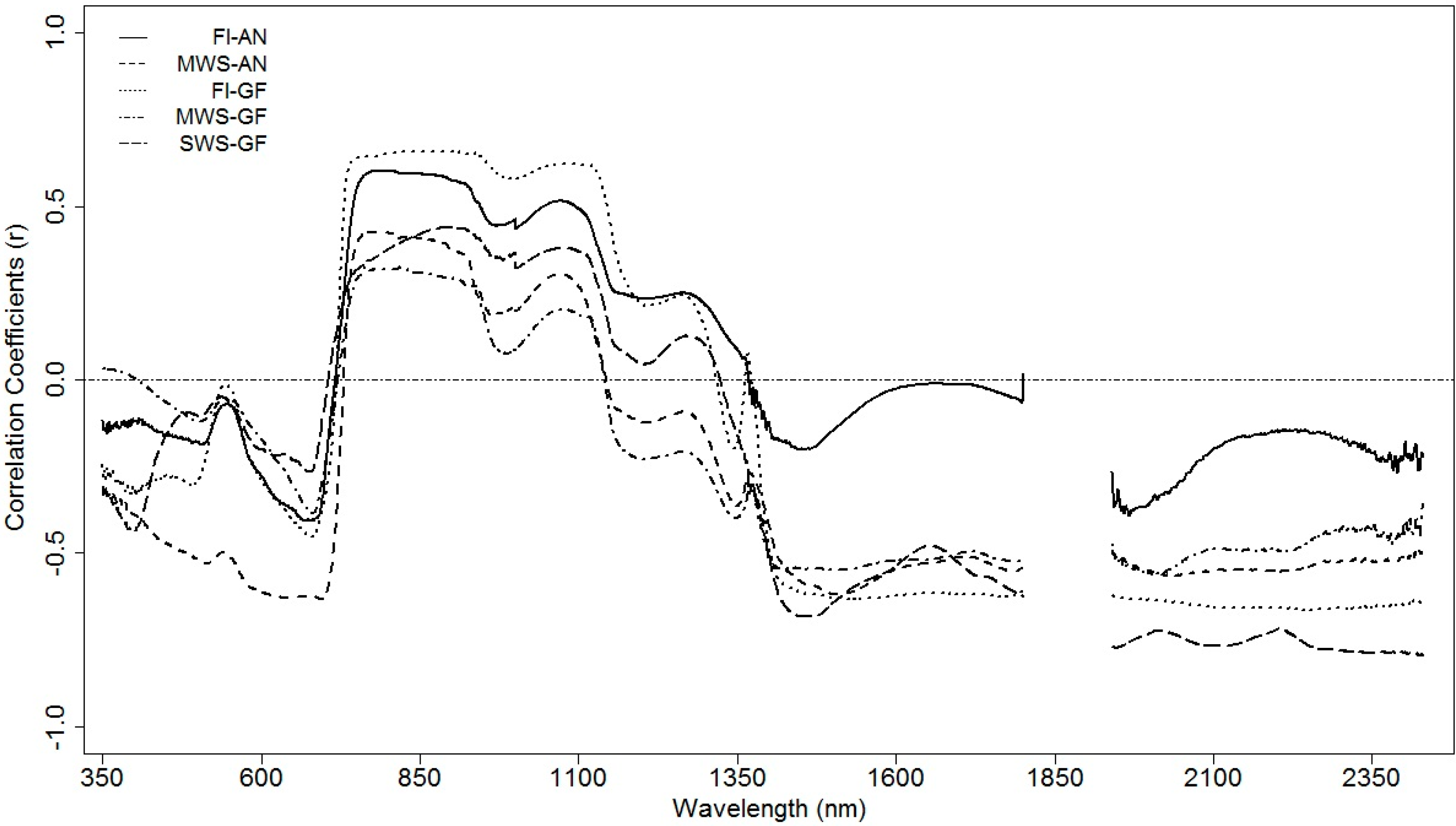
3.1. Relationship between Spectral Signature and Grain Yield

Mean GY was reduced by 79% and 41% under SWS and MWS, respectively, compared to GY under full irrigation (Table 1). The highest standard deviation and the lowest coefficient of variation were observed in FI, but the opposite occurred in SWS. Significant Pearson correlations were found between the GY of the 368 wheat genotypes in single wavelengths (Figure 1). In the visible zone of the spectrum (400 to 700 nm), the correlation values were negative in all environments; MWS measured at AN had the highest mean value (R = −0.55). In the near-infrared (NIR) zone, the area included between 700 and 1100 nm, the R values were positive in all environments; under FI at the GF stage the R values were on average 0.63. In the shortwave infrared zone (SWIR, 1100 and 1300 nm), changes in the signs depended on the environment; (1) positive correlation in FI-AN, FI-GF and SWS-GF, and (2) negative relationships in MWS-AN and MWS-GF. Negative correlation coefficients were found in all environments at wavelengths higher than 1400 nm; under SWS at the GF stage the correlation was the strongest (R = −0.65).
Table 1. Main statistical parameters of grain yield for the 368 genotypes growing under three water regimes.
VariableNMean Kg∙ha−1Min Kg∙ha−1Max Kg∙ha−1SD Kg∙ha−1CV (%)
Severe Stress39116551304394696.142.1
Medium Stress3994739607101441425.830.1
Full Irrigation39779672240129921788.422.5
N: number of samples, Mean: grain yield average, Min: minimum grain yield, Max: maximum grain yield, SD: standard deviation, CV: coefficient of variation. Mean, Min, Max, SD and CV in kg·ha−1. Severe Stress (SV), Medium Stress (MS) and Full Irrigation (FI) correspond to three water conditions.
Figure 1. Pearson’s coefficient of correlation (R) between grain yield and wavelengths measured at anthesis (AN) and grain filling (GF) under severe water stress (SWS), medium water stress (MWS) and full irrigation (FI).
Remotesensing 07 02109 g001
When the spectral signatures of the 15 genotypes with the highest and lowest GY were compared under each water regime, clear differences in the reflectance of certain wavelengths were observed (Figure 2). With the exception of SWS, genotypes with the highest GY exhibited lower reflectance values between 400 and 750 nm; these differences were clearly observed in MWS measured at anthesis. Under FI, no substantial differences in reflectance were observed in the two growing stages close to 550 nm. However, under MWS, differences in reflectance were evident, particularly at anthesis. Differences were less obvious for SWS as compared with the other water regimes and presented opposite tendencies to MWS with higher values for high-yield genotypes of the zone correspondent to close at 550 nm. Reflectance corresponding to the red edge (700 to 800 nm) also contrasted between the top high-yielding and lower-yielding genotypes (Figure 2), where higher reflectance values were observed in high-yielding genotypes. For the NIR region between 800 and 1200 nm, reflectance was higher in the genotypes with the highest yields; on the average, FI demonstrated the highest values on both dates. In the SWIR wavelengths (1200 to 2400 nm), high-yield genotypes under the three water regimes generally exhibited lower mean reflectance for this area as compared with low-yield genotypes.
Figure 2. Standard normal variation (SNV) reflectance of 15 genotypes with the highest (HY) and lowest (LY) yields determined at the anthesis (a) and grain filling (b) stages, under severe water stress (SWS), medium water stress (MWS) and full irrigation (FI).
Remotesensing 07 02109 g002

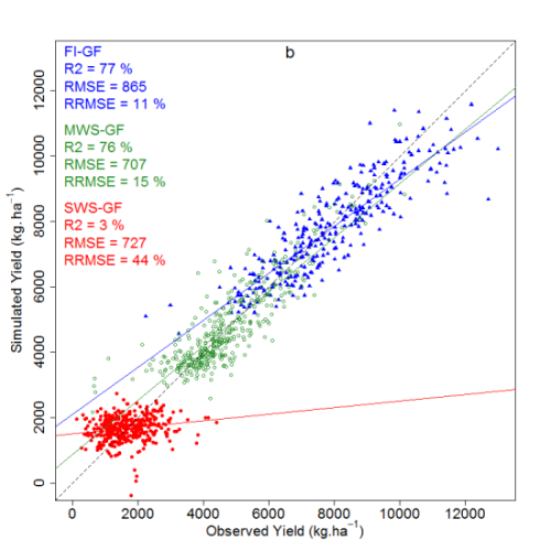
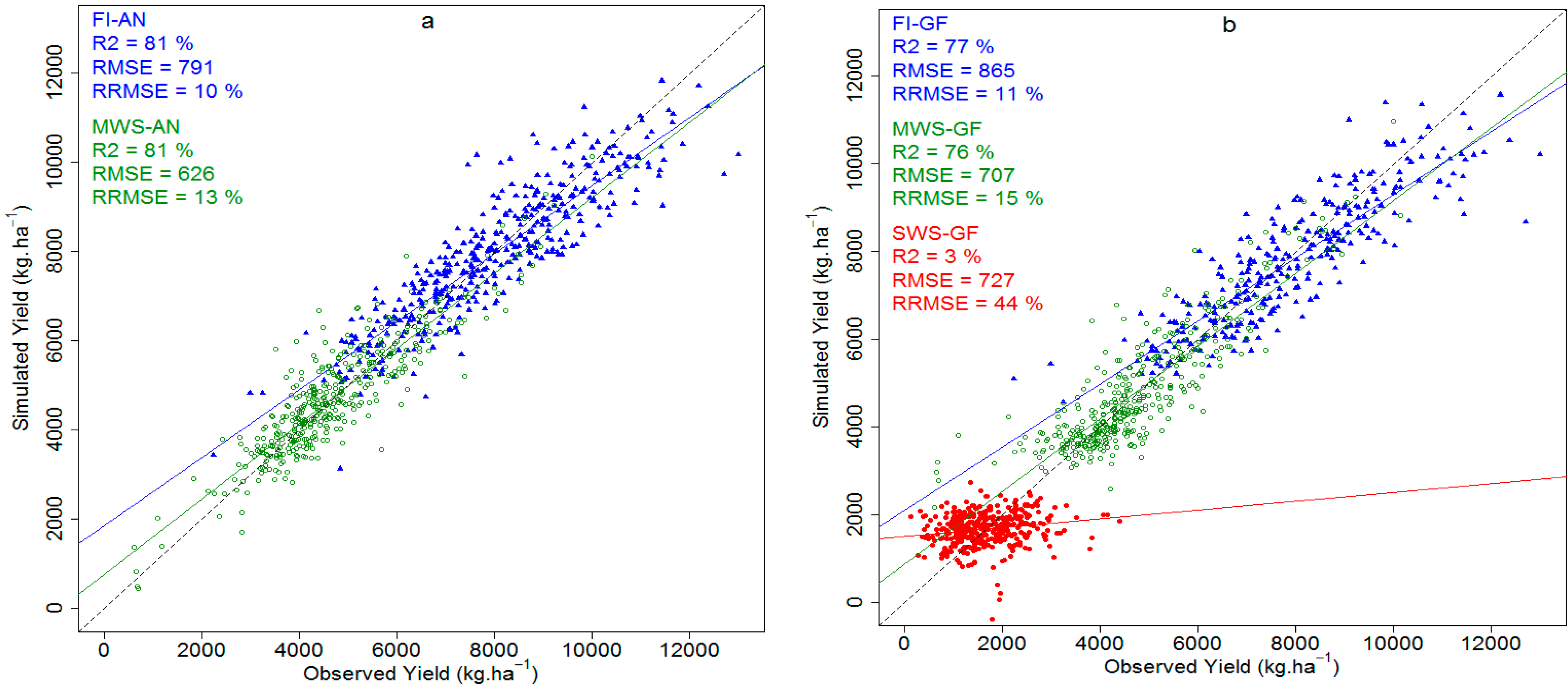
3.2. Prediction with the Ridge Regression Model

The results showed that models generated by ridge regression explained between 77% and 91% of yield variability in the three water regimes and phenological stages (Table 2). Values of the coefficient of determination (R2) for GY were higher under MWS (R2 = 0.88) at anthesis and under SWS (R2 = 0.91) at grain filling. The highest coefficient of determination occurred under SWS at the GF stage. The most extreme RMSE values were 210 and 809 kg∙ha−1 for SWS-GF and FI-AN, respectively. The highest rRMSE values were obtained in both stress conditions (MWS and SWS) at grain filling with 14.4% and 12.7%, respectively. The lowest rRMSE values were found in FI independently of the phenological stage. Combined models explained between 90% and 92% of the variation in predicting grain yield (Table 2) at AN and GF, respectively.
Table 2. The most important statistics obtained from the Ridge Regression models to estimate yields based on the spectral signature in each plot.
ModelnLambdaR2 (%)RMSE (kg∙ha−1)rRMSE (%)
Anthesis
FI39756.78080910.2
MWS3993.88849810.5
FI-MWS7964.19071111.2
Grain Filling
FI3013.8837259.2
MWS39920.77768414.4
SWS3912.19121012.7
FI-MWS-SWS10911.19276016.8
n: number of samples; lambda: model penalization value; R2: model coefficient of determination; RMSE (kg∙ha−1): root mean square error; rRMSE: ratio between RMSE and yield. Data correspond to all environments (FI: full irrigation, MWS: medium water stress, SWS: severe water stress), and phenological stages (AN: anthesis and GF: grain filling).
When the relative weight of the regression coefficients resulting from the ridge regression model (Figure 3) was analyzed, there was variability in the magnitude of coefficients for the different wavelengths that was dependent on both the water regime and phenological stages. For wavelengths between 400 and 750 nm, model coefficients were both positive and negative for the two phenological stages. All the models in this zone had positive regression coefficient values for wavelengths from 480 to 550 nm. In contrast, the 550 to 570 nm zone had negative values under SWS at GF and positive values under FI at AN. In the red edge zone (700 to 800 nm), coefficient values were negative in all water regimes, however, in the GF stage under MWS, values were negative but became positive from 740 nm onwards. Coefficients in FI were negative in the reflectance area between 950 and 1000 nm and positive for SWS; the sign of the coefficients was maintained in both development stages. In the 1100 to 2500 nm zone, coefficient values were found to depend on both water regime and phenological stage. At 1100 nm, coefficients at anthesis were close to 0 under FI and MWS; however, values were positive in the three water regimes when measured at GF. At 1240 nm, irrigated environments at both development stages had values close to 0, but were negative under water stress conditions. No clear pattern was observed in any environment or phenological stage for wavelengths between 2000 and 2400 nm.
The regression coefficients of each combined model were later used to predict the GY in the water regime from which they had been generated (Figure 4). The comparison resulted in an R2 of 81% under FI and MWS respectively, at anthesis, whereas it was 77% and 76% under FI and MWS at grain filling. However, yield prediction using the combined model generated during grain filling was not significant under SWS.
Figure 3. Relative weight of regression coefficients for each wavelength. Coefficients have been re-scaled, dividing them by the maximum absolute value for each model in order to simplify the comparison Data correspond to all environments (FI: full irrigation, MWS: medium water stress, SWS: severe water stress), and phenological stages ((a) AN: anthesis and (b) GF: grain filling). Coefficients were generated after the calibration of each environmental and phenological stage.
Remotesensing 07 02109 g003
Figure 4. Comparison of observed grain yield (kg∙ha−1) by using regression coefficients of combined models for the phenological stages of (a) anthesis and (b) grain filling. R2: coefficient of determination, RMSE: Root Mean Squared Error, rRMSE: Relative Root Mean Squared Error, red dots correspond to SWS, green dots to MWS, and blue dots to FI.
Remotesensing 07 02109 g004
Model robustness was then evaluated for each water regime and phenological stage by applying each model to the other conditions and stages (Table 3). In this case, both water regime and development stage exhibited differences in the ability to predict GY. In general, most of the models achieved an acceptable yield prediction in other environmental conditions. The highest correlation value was found for the SWS-GF model applied to MWS-GF, while the lowest value was for MWS-GF applied to FI-AN. It was observed that models generated at anthesis usually have a greater ability to predict yield as compared with models generated at grain filling. Low and medium yield environments also show a better correlation between observed and predicted yields. Although the correlation coefficient values tend to be higher in most of the cases evaluated, rRMSE values for these models were much higher than those found in individual and combined models. In the model generated, SWS-GF showed the highest rRMSE values in all the environments where it was applied.
Table 3. Coefficients of correlation of individual models applied to different environments. Coefficients of regression generated by each water regime (SWS, MWS and FI) and phenological stage (AN and GF) were used for yield predictions in the different conditions.
ModelFI-ANMWS-ANFI-GFMWS-GFSWS-GF
RrRMSE (%)RrRMSE (%)RrRMSE (%)RrRMSE (%)RrRMSE (%)
FI-AN *0.77 ***530.56 ***190.69 ***540.43 ***132
MWS-AN *0.66 ***550.56 ***540.76 ***190.68 ***99
FI-GF *0.67 ***220.46 ***540.65 ***540.71 ***136
MWS-GF *0.02 ns650.18 **430.31 ***620.67 ***104
SWS-GF *0.46 ***1370.43 ***1070.25 **1360.78 ***102
* p < 0.05; ** p < 0.01; *** p < 0.001; ns = non-significant. * Models’ regression coefficients applied to different environments and phenological stages.

3.3. Prediction with Spectral Vegetation Indices

The spectral vegetation indices were calculated and used to predict wheat grain yield. The predictive power was lower than the prediction by the Ridge model with R2 values between 0% and 62% (Table 4). The PRI under FI-GF and MWS-GF were not significantly correlated. The WI generally showed the highest predictive ability with significant correlations for all phenological stages and environments, with R2 between 56% and 69%. At FI-AN and SWS-GF the spectral vegetation indices showed the minimum R2 values to predict grain yield correctly. However, when spectral information from water regimes was combined within a phenological stage, the vegetation indices with the highest values were NDVI and WI (R2 > 80%) during grain filling. Finally, in the MWS environment, for both AN and GF, the predictive power of the indices was higher than for the other environmental conditions (Table 4).

3.4. Discussion

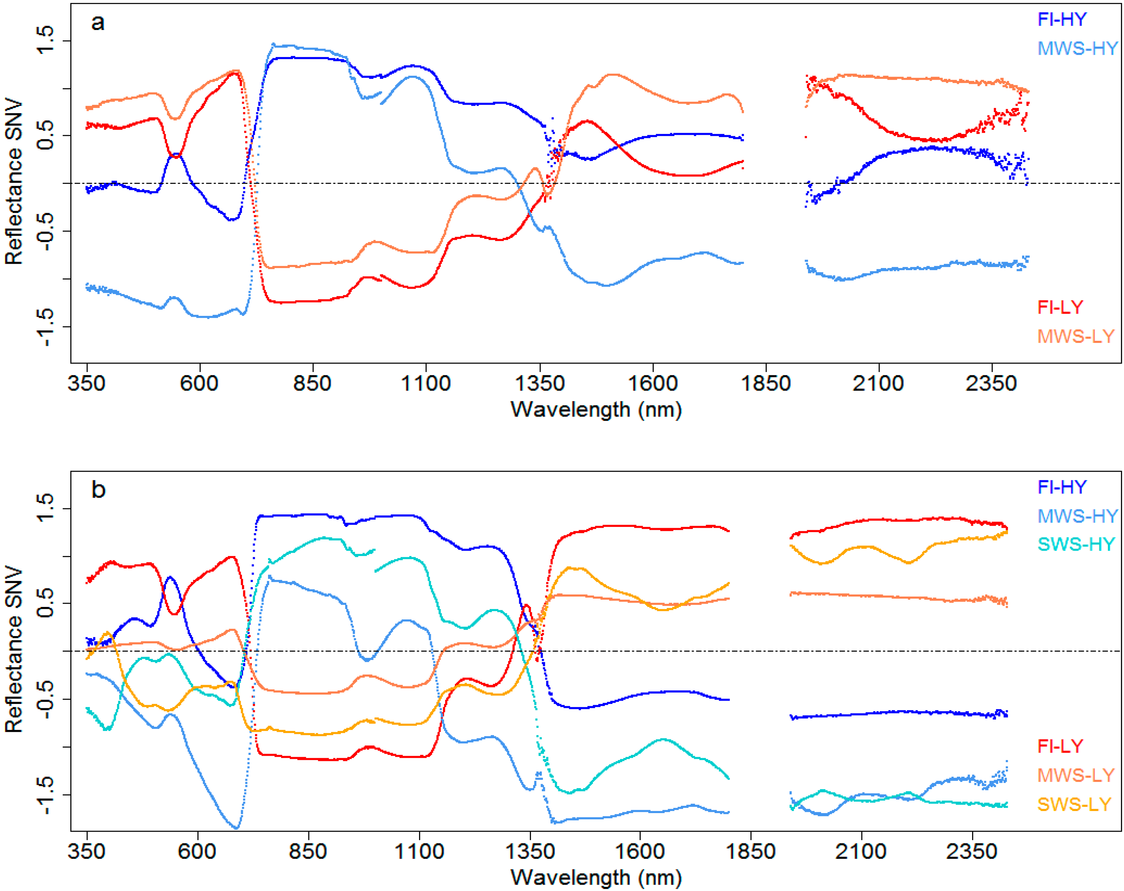
3.4.1. Canopy Reflectance in Genotypes of Contrasting Grain Yield

Reflectance values were measured by field spectroradiometry for wavelengths between 400 and 2500 nm in the 368 genotypes in different environments and at different development stages and were similar to those reported in wheat and barley grown with and without stress for different development stages [37,39]. High-yield genotypes reflected a lower amount of radiation in the visible spectrum (400–700 nm) as compared with low-yield genotypes, and this could be related to the leaf content of anthocyanins, carotenoids and chlorophyll, which are lower as a consequence of water stress [10,40]. As reported by Penuelas et al. [41], lower reflectance in the visible spectrum was associated with higher chlorophyll content. Also, Zhao et al. [42] reported higher reflectance in the 550–710 nm zone in a maize crop with an N deficit. However, other studies [37,43] revealed lower reflectance in the red zone associated with higher rates of N fertilization in wheat plants.
Table 4. Relationships of spectral vegetation indices measured at anthesis and grain filling in three water conditions to grain yield. Values are expressed as coefficient of determination (R2).
ModelNDVIPRIWISR
R2 (%)R2 (%)R2 (%)R2 (%)
Anthesis
FI23.3 ***25.2 ***55.8 ***23.8 ***
MWS34.1 ***42.6 ***55.9 ***40.2 ***
FI-MWS37.9 ***50.8 ***69.0 ***45.3 ***
Grain filling
FI28.8 ***0.0 NS51.3 ***14.9 ***
MWS47.9 ***0.0 NS62.7 ***38.8 ***
SWS35.7 ***22.1 **54.1 ***30.1 ***
FI-MWS-SWS79.8 ***0.0 NS79.8 ***53.0 ***
* p < 0,05; ** p < 0,01; *** p < 0,001; ns = non-significant.
In the NIR zone (800 to 1300 nm), high-yield genotypes showed higher reflectance in all environments, which could be associated with a greater leaf area index and green biomass [44,45]. Between 930 and 970 nm, the lowest reflectance value found for MWS was probably related to the canopy’s water content [46]. In MWS and SWS environments, there was an increase in reflectance in this zone due to lower water content. The inverse phenomenon was observed for FI environments (Figure 2). In the SWIR region, some bands have been associated with water absorption [16]. In this zone, low-yield genotypes exhibited higher reflectance and these differences were increased under stress conditions (MWS and SWS), which suggest that water can influence the reflectance measurements. Seelig et al. [16] indicated that the 1200, 1450, 1930 and 2500 nm wavelengths exhibited a significant correlation with leaf water content, however, some wavelengths had high variability. It should be clearly noted that the estimates of grain yield are achieved by assessing the state of the whole plant, and the relationship between these variables and yield is indirect.

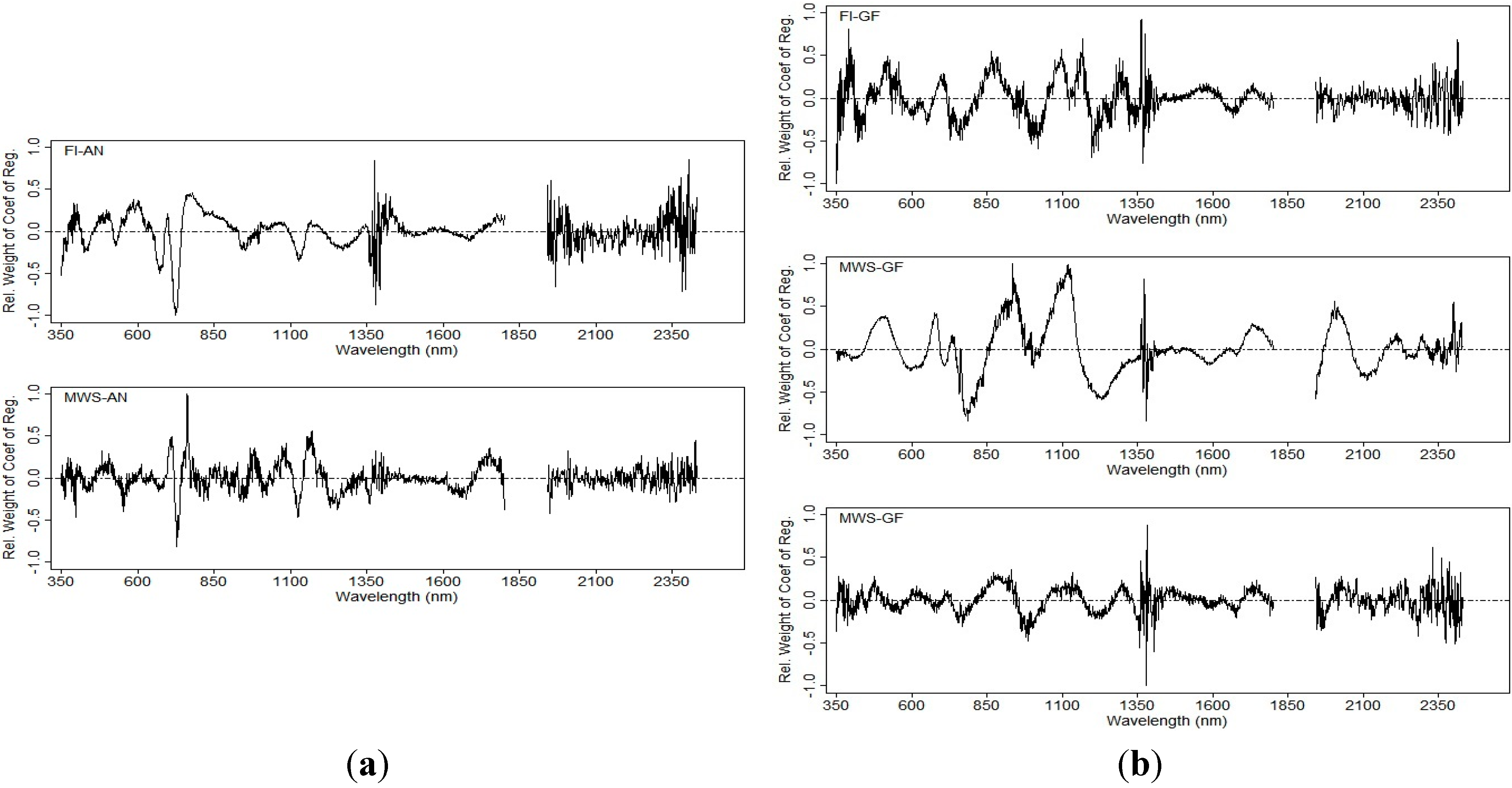
3.4.2. Regression Coefficients for Different Spectral Zones

The highest regression coefficients in the models generated by ridge regression for each wavelength (Figure 3) were found in zones previously related to reflectance studies on chlorophyll content (680 and 550 nm) and carotenoids (480 nm) [42], leaf area index and biomass (680 to 980 nm), [44], water content (930 to 970 nm) [47], and SWIR (1300 to 1450 nm) [16]. Under FI and MWS the coefficient values in the 680 nm zone were negative at anthesis and changed to positive at grain filling, whereas at 550 nm the values were the opposite between FI and MWS conditions for the same phenological stage. For the spectral zone associated with brown pigment content (750 and 800 nm) [20], coefficient values were positive under FI and MWS conditions at anthesis. However, when the quantity of these compounds increased at grain filling, the coefficient values tended to be negative in the three environments (FI, MWS, SWS). This indicates that the model was able to separate between phenological stages through differences in these compounds (Figure 3). In the NIR region, changes in reflectance related to N content and aerial biomass reported in maize [48] were also present in the regression coefficients; during anthesis, positive values around 800 nm become negative at 900 nm in FI and to a lesser extent in MWS. This contrasts with measurements at grain filling where negative values became positive in both water stress conditions and to a lesser extent in FI. These variations in magnitude and sign of the coefficients could account for changes in the canopy because this zone has been related to differences in the canopy’s biomass during measurements between anthesis and grain filling [37,43].
In the case of NIR wavelengths associated with canopy water content [47], regression coefficients during anthesis showed that FI and MWS environments have values close to 0, while MWS, SWS, and to a lesser degree optimum irrigation, have positive and high coefficient values at grain filling. This coincides with Peñuelas et al. [46], who found that declines in reflectance in the zone between 930 and 970 nm are correlated with canopy water content. In addition, differences were found in the regression coefficient values for the SWIR zone, which has been associated with water content and absorbance. Negative coefficient values were observed under FI and MWS environments in the spectral zone between 1100 and 1140 nm. However, when measured at grain filling, both water regimes exhibited positive values, with the exception of SWS, which had values close to 0. Sims and Gamon [49] stated that these zones are directly correlated with water content in plants under field conditions. In the 1240 to 1260 nm zone, coefficients were negative in both stages and under the three water regimes. Reflectance measurements taken during the grain-filling period, when plant water content is an important factor for development, can be used as a selection criterion.
In summary, genotypes with low reflectance in the visible wavelengths (VIS) (400 to 700 nm), high reflectance in the NIR (750 to 1100 nm), and low reflectance in the SWIR (1300 to 2400 nm), which are associated with high photosynthetic capacity, biomass, and water content, tend to have higher GY. Various studies in wheat have associated GY with reflectance data from these zones of the spectral signature [17,21,50].

3.4.3. Grain Yield Prediction Using Multivariate Models

Although the ridge regression models are empirical approaches, they show good correlations with GY and integrate morpho-physiological information that determines GY [51,52]. At anthesis, the best model was under MWS, and this was probably due the greater GY variability (CV = 30.1%), which increases the magnitude of the data variation and improves the predictive ability of the model [25]. At grain filling, the highest R2 occurred under SWS, which can be explained by Figure 1 where a high correlation exists between the SWIR zone (associated with water content) and GY. Thus, under terminal drought conditions, those genotypes that reach grain filling with the greatest plant water content attain higher GY. Combined models showed higher R2 than individual models, suggesting that integrating a greater amount of measurement information improves predictive capacity. This slight increase in the estimate could be due to the presence of more information in the model for the number of environments (2) as well as the number of evaluated genotypes (368), which represents a substantial number for these types of studies. When data from the combined models were used to predict GY within individual trials, coefficients of determination were generally high, but still lower than the individual models (Figure 4). Combined models generated during anthesis resulted in R2 values that decreased the capacity to predict GY by 8% in comparison to the individual models.
When the combined model generated during grain filling was used to predict yield in the individual trials, decreases of 76% and 77% under MWS and FI conditions, respectively, were observed. However, this decrease was higher under SWS during grain filling and declined to only 3% of the capacity to predict GY. This could be due to the fact that in MWS and FI the chlorophyll content, biomass, and leaf area index are components that indicate different levels of water stress, thus, when these variables are higher the yield is higher. Nevertheless, in an environment with severe water limitations, the most significant factor is the plant’s water capacity, such as the canopy water content until the end of the period of growing (grain filling). Although it is possible to generate combined models between different environments, interactions produced among genotypes and the environment cannot be overlooked because the traits being used to achieve GY predictions are different between environments. These differences are not considered when generating the prediction because an empirical model is being used. A similar situation was observed by Weber et al. [24] in maize where a decrease in the capacity to predict GY was found when using regression coefficients of combined models in the environments that generated them.
When individual models were used to predict grain yield in other conditions, MWS during anthesis was the best model to predict GY. This could be due to the existence of higher variability at this stage in chlorophyll content, biomass, and water content together with a greater expression of yield variability among the evaluated genotypes compared to the other environments, for example the MWS-GF where low predictive capacity was observed. The rRMSE values for all models were much higher than the data from the individual models. One of the main limitations of using models generated for different environmental conditions and different phenological stages is that they cannot be used without a detailed calibration and corresponding validations

3.4.4. Comparison between the Spectral Vegetation Indices and Ridge Regression Predictions

The yield predictive capacity of the spectral vegetation indices was lower than the Ridge model for all the environments and phenological stages (Table 4). However, strong correlations were obtained for NDVI and WI, particularly when all environments in grain filling were included. Similar results were obtained by Royo et al. [21] with R2 values higher than 80% for the same vegetation indices, but only during anthesis. In the current research, the WI produces good predictions in both phenological stages, but with an R2 of 80% during grain filling. In general terms, the WI exhibited a strong correlation with grain yield compared to the rest of the spectral vegetation indices. These results demonstrated that for the set of genotypes tested the biophysical response of plants, which is explained as the changes in the spectral signatures, was mainly related to water content in the plants cells as represented by the WI. These results respond to the great variability in the drought conditions to which the plants were exposed. The different abilities of vegetation indices to predict grain yield demonstrates the low stability in predicting GY under different environment and phenological conditions, but this is not the case when Ridge regression is applied.
The different environments generate variable predictive conditions, with MWS having the best adjustments among all the indices. The MWS data set exhibited the most important variability in terms of the different wavelength used for each index. Regressions were thus constructed with an ample range of information from the spectral data, which responded to the different morpho-physiological traits found in the intermediate stress environment. However, this phenomenon did not occur in the same way for the FI and SWS environments, which had more extreme environmental conditions, and the spectral data set considered by the indices was not sufficiently variable among the 368 genotypes. Therefore, the morpho-physiological response of the genotypes was more homogeneous.
Ridge predictions were robust for all environments and exhibited a high adjustment with values always greater than 77% (Table 2). These results indicate the method’s sensitivity for capturing small spectral variations in genotypes exposed to extreme environmental conditions. Similar results were found by Weber et al. [24] and Ferrio et al. [25], who used methods from multivariate regressions and who also demonstrated results that were more robust than conventional spectral indices. Both studies used the PLSR method and generated predictions with coefficients of determination (R2) between 16% and 76% [25] and 69% and 71% [24], which were lower values than the ridge regression model used with our data set.

4. Conclusions

Canopy reflectance measurements represent a relevant source of information because some wavelengths are directly related to morpho-physiological processes. The information provided by field spectroradiometry at different stages and under different water regimes allows prediction of yields over a wide set of different genotypes. Different genotypes vary in their response according pigment concentrations, biomass, and water content, which are key parameters that define the optical properties of the canopy.
The ridge regression models were able to estimate genotype yields for different irrigation conditions and physiological stages. Better predictions were obtained using all the wavelengths of the canopy reflectance spectrum in different environments when compared to conventional yield predictions based on spectral indices. Models that integrated all the information for a specific phenological stage were usually more robust at determining yield than individual models. Results suggest that the most accurate genotype prediction is achieved at the anthesis stage, but further evaluation must be performed during anthesis at SWS in order to complete the data set for all conditions. Finally, this technique could be suitable to predict grain yield among different genotypes in high and low-yield environments. However, during grain filling, the combined model showed poor results in SWS conditions. Indeed, it should be noted that the information generated is highly dependent on the environment where measurements are taken, so these data must be re-evaluated in a wide range of environments and genotypes to generate the most robust models possible.

Acknowledgments

The authors would like to thank Julio di Rienzo of the University of Cordova for his technical assistance in data management and analysis of the spectral data. This work was supported by the research grant FONDECYT N° 1110732, FONDEQUIP 130073, and the research program “Adaptation of Agriculture to Climate Change (A2C2)” from Universidad de Talca, Chile.

Author Contributions

Javier Hernandez processed and analyzed the data and wrote the manuscript. Gustavo A. Lobos led the study and collected field data and spectral data in Chillan and Cauquenes and contributed to the writing of the manuscript. Ivan Matus provided germplasm for the experiments and supervised the field activities in Chillan and Cauquenes. Alejandro del Pozo helped in the design of the experiment, collected field and spectral data and contributed to the writing of the manuscript. Paola Silva contributed to the writing of the manuscript. Mauricio Galleguillos processed and analyzed the data, contributed to the writing of the manuscript and discussed the results and statistical analysis.

Conflicts of Interest

The authors declare no conflict of interest.

References

  1. Araus, J.L.; Slafer, G.A.; Royo, C.; Serret, M.D. Breeding for yield potential and stress adaptation in cereals. Crit. Rev. Plant Sci. 2008, 27, 377–412. [Google Scholar] [CrossRef]
  2. Fleury, D.; Jefferies, S.; Kuchel, H.; Langridge, P. Genetic and genomic tools to improve drought tolerance in wheat. J. Exp. Bot. 2010, 61, 3211–3222. [Google Scholar] [CrossRef] [PubMed]
  3. Reynolds, M.; Pask, A.; Mullan, D. Physiological Breeding I: Interdisciplinary Approaches to Improve Crop Adaptation; International Maize and Wheat Improvement Center (CIMMYT): Texcoco, Mexico, 2012. [Google Scholar]
  4. Cattivelli, L.; Rizza, F.; Badeck, F.-W.; Mazzucotelli, E.; Mastrangelo, A.M.; Francia, E.; Mare, C.; Tondelli, A.; Stanca, A.M. Drought tolerance improvement in crop plants: An integrated view from breeding to genomics. Field Crops Res. 2008, 105, 1–14. [Google Scholar] [CrossRef]
  5. Araus, J.L.; Slafer, G.A.; Reynolds, M.P.; Royo, C. Plant breeding and drought in c3 cereals: What should we breed for? Ann. Bot. 2002, 89, 925–940. [Google Scholar] [CrossRef] [PubMed]
  6. Araus, J.L.; Serret, M.D.; Edmeades, G.O. Phenotyping maize for adaptation to drought. Front. Physiol. 2012, 3, 1–20. [Google Scholar] [CrossRef] [PubMed] [Green Version]
  7. Reynolds, M.; Mujeeb-Kazi, A.; Sawkins, M. Prospects for utilising plant-adaptive mechanisms to improve wheat and other crops in drought-and salinity-prone environments. Ann. Appl. Biol. 2005, 146, 239–259. [Google Scholar] [CrossRef]
  8. Araus, J.L.; Cairns, J.E. Field high-throughput phenotyping: The new crop breeding frontier. Trends Plant Sci. 2014, 19, 52–61. [Google Scholar] [CrossRef] [PubMed]
  9. White, J.W.; Andrade-Sanchez, P.; Gore, M.A.; Bronson, K.F.; Coffelt, T.A.; Conley, M.M.; Feldmann, K.A.; French, A.N.; Heun, J.T.; Hunsaker, D.J. Field-based phenomics for plant genetics research. Field Crops Res. 2012, 133, 101–112. [Google Scholar] [CrossRef]
  10. Hatfield, J.; Gitelson, A.A.; Schepers, J.S.; Walthall, C. Application of spectral remote sensing for agronomic decisions. Agron. J. 2008, 100, S117–S131. [Google Scholar] [CrossRef]
  11. Blackburn, G.A. Hyperspectral remote sensing of plant pigments. J. Exp. Bot. 2007, 58, 855–867. [Google Scholar] [CrossRef] [PubMed]
  12. Royo, C.; Villegas, D. Field measurements of canopy spectra for biomass assessment of small-grain cereals. In Biomass-Detection, Production and Usage; Matovic, D., Ed.; INTECH: Rijeka, Croatia, 2011; pp. 27–52. [Google Scholar]
  13. Sims, D.A.; Gamon, J.A. Relationships between leaf pigment content and spectral reflectance across a wide range of species, leaf structures and developmental stages. Remote Sens. Environ. 2002, 81, 337–354. [Google Scholar] [CrossRef]
  14. Garriga, M.; Retamales, J.B.; Romero, S.; Caligari, P.D.S.; Lobos, G.A. Chlorophyll, anthocyanin and gas exchangechanges assessed by spectroradiometry in fragaria chiloensis under salt stress. J. Integr. Plant Biol. 2014, 56, 505–515. [Google Scholar] [CrossRef] [PubMed]
  15. Liu, J.; Pattey, E.; Miller, J.R.; McNairn, H.; Smith, A.; Hu, B. Estimating crop stresses, aboveground dry biomass and yield of corn using multi-temporal optical data combined with a radiation use efficiency model. Remote Sens. Environ. 2010, 114, 1167–1177. [Google Scholar] [CrossRef]
  16. Seelig, H.D.; Hoehn, A.; Stodieck, L.S.; Klaus, D.M.; Adams Iii, W.W.; Emery, W.J. The assessment of leaf water content using leaf reflectance ratios in the visible, near-, and short-wave-infrared. Int. J. Remote Sens. 2008, 29, 3701–3713. [Google Scholar] [CrossRef]
  17. Aparicio, N.; Villegas, D.; Casadesus, J.; Araus, J.L.; Royo, C. Spectral vegetation indices as nondestructive tools for determining durum wheat yield. Agron. J. 2000, 92, 83–91. [Google Scholar] [CrossRef]
  18. Lobos, G.A.; Matus, I.; Rodriguez, A.; Romero-Bravo, S.; Araus, J.L.; del Pozo, A. Wheat genotypic variability in grain yield and carbon isotope discrimination under mediterranean conditions assessed by spectral reflectance. J. Integr. Plant Biol. 2014, 56, 470–479. [Google Scholar] [CrossRef] [PubMed]
  19. Araus, J.L. Integrative physiological criteria associated with yield potential. In Increasing Yield Potential in Wheat: Breaking the Barriers; Reynolds, M.P., Rajaram, S., McNab, A., Eds.; International Maize and Wheat Improvement Center (CIMMYT): Texcoco, Mexico, 1996; pp. 150–167. [Google Scholar]
  20. Peñuelas, J.; Filella, I. Visible and near-infrared reflectance techniques for diagnosing plant physiological status. Trends Plant Sci. 1998, 3, 151–156. [Google Scholar] [CrossRef]
  21. Royo, C.; Aparicio, N.; Villegas, D.; Casadesus, J.; Monneveux, P.; Araus, J.L. Usefulness of spectral reflectance indices as durum wheat yield predictors under contrasting mediterranean conditions. Int. J. Remote Sens. 2003, 24, 4403–4419. [Google Scholar] [CrossRef]
  22. Graeff, S.; Claupein, W. Quantifying nitrogen status of corn (Zea mays L.) in the field by reflectance measurements. Eur. J. Agron. 2003, 19, 611–618. [Google Scholar] [CrossRef]
  23. Hansen, P.; Schjoerring, J. Reflectance measurement of canopy biomass and nitrogen status in wheat crops using normalized difference vegetation indices and partial least squares regression. Remote Sens. Environ. 2003, 86, 542–553. [Google Scholar] [CrossRef]
  24. Weber, V.S.; Araus, J.L.; Cairns, J.E.; Sanchez, C.; Melchinger, A.E.; Orsini, E. Prediction of grain yield using reflectance spectra of canopy and leaves in maize plants grown under different water regimes. Field Crops Res. 2012, 128, 82–90. [Google Scholar] [CrossRef]
  25. Ferrio, J.P.; Villegas, D.; Zarco, J.; Aparicio, N.; Araus, J.L.; Royo, C. Assessment of durum wheat yield using visible and near-infrared reflectance spectra of canopies. Field Crops Res. 2005, 94, 126–148. [Google Scholar] [CrossRef]
  26. Hastie, T.; Tibshirani, R.; Friedman, J.; Franklin, J. The elements of statistical learning: Data mining, inference and prediction. Math. Intell. 2005, 27, 83–85. [Google Scholar]
  27. Lazaridis, D.C.; Verbesselt, J.; Robinson, A.P. Penalized regression techniques for prediction: A case study for predicting tree mortality using remotely sensed vegetation indices this article is one of a selection of papers from extending forest inventory and monitoring over space and time. Can. J. For. Res. 2010, 41, 24–34. [Google Scholar] [CrossRef]
  28. Cai, T.; Ju, C.; Yang, X. Comparison of ridge regression and partial least squares regression for estimating above-ground biomass with landsat images and terrain data in mu us sandy land, China. Arid Land Res. Manag. 2009, 23, 248–261. [Google Scholar] [CrossRef]
  29. Tikhonov, A. On the stability of inverse problems. Proc. URSS Acad. Sci. 1943, 39, 195–198. [Google Scholar]
  30. Hoerl, A.E.; Kennard, R.W. Ridge regression: Applications to nonorthogonal problems. Technometrics 1970, 12, 69–82. [Google Scholar] [CrossRef]
  31. Stolpe, N. Descripciones de los Principales Suelos de la Octava Región de Chile; Universidad de Concepción,Facultad de Agronomía: Chillán, Chile, 2006. [Google Scholar]
  32. Del Pozo, A.; del Canto, P. Características del Valle Central: Áreas Agroclimáticas y Sistemas Productivos en las VII y VIII Regiones; Instituto de Investigaciones Agropecuarias,Centro Regional de Investigación Quilamapu: Chillan, Chile, 1999. [Google Scholar]
  33. Zadoks, J.C.; Chang, T.T.; Konzak, C.F. A decimal code for the growth stages of cereals. Weed Res. 1974, 14, 415–421. [Google Scholar] [CrossRef]
  34. Randolph, T.W. Scale-based normalization of spectral data. Cancer Biomark. 2006, 2, 135–144. [Google Scholar] [PubMed]
  35. Serrano, L.; Ustin, S.L.; Roberts, D.A.; Gamon, J.A.; Peñuelas, J. Deriving water content of chaparral vegetation from AVIRIS data. Remote Sens. Environ. 2000, 74, 570–581. [Google Scholar] [CrossRef]
  36. Venables, W.N.; Ripley, B.D. Modern Applied Statistics with S; Springer: New York, NY, USA, 2002. [Google Scholar]
  37. Serrano, L.; Filella, I.; Peñuelas, J. Remote sensing of biomass and yield of winter wheat under different nitrogen supplies. Crop Sci. 2000, 40, 723–731. [Google Scholar] [CrossRef]
  38. R Development Core Team. R: A Language and Environment for Statistical Computing; R Foundation for Statistical Computing: Vienna, Austria, 2012. [Google Scholar]
  39. Peñuelas, J.; Inoue, Y. Reflectance indices indicative of changes in water and pigment contents of peanut and wheat leaves. Photosynthetica 1999, 36, 355–360. [Google Scholar] [CrossRef]
  40. Gitelson, A.A.; Chivkunova, O.B.; Merzlyak, M.N. Nondestructive estimation of anthocyanins and chlorophylls in anthocyanic leaves. Am. J. Bot. 2009, 96, 1861–1868. [Google Scholar] [CrossRef] [PubMed]
  41. Penuelas, J.; Gamon, J.A.; Griffin, K.L.; Field, C.B. Assessing community type, plant biomass, pigment composition, and photosynthetic efficiency of aquatic vegetation from spectral reflectance. Remote Sens. Environ. 1993, 46, 110–118. [Google Scholar] [CrossRef]
  42. Zhao, D.; Raja Reddy, K.; Kakani, V.G.; Read, J.J.; Carter, G.A. Corn (Zea mays L.) growth, leaf pigment concentration, photosynthesis and leaf hyperspectral reflectance properties as affected by nitrogen supply. Plant Soil 2003, 257, 205–218. [Google Scholar] [CrossRef]
  43. Filella, I.; Serrano, L.; Serra, J.; Peñuelas, J. Evaluating wheat nitrogen status with canopy reflectance indices and discriminant analysis. Crop Sci. 1995, 35, 1400–1405. [Google Scholar] [CrossRef]
  44. Peñuelas, J.; Isla, R.; Filella, I.; Araus, J.L. Visible and near-infrared reflectance assessment of salinity effects on barley. Crop Sci. 1997, 37, 198–202. [Google Scholar] [CrossRef]
  45. Peñuelas, J.; Filella, I.; Serrano, L.; Savé, R. Cell wall elasticity and water index (r970 nm/r900 nm) in wheat under different nitrogen availabilities. Int. J. Remote Sens. 1996, 17, 373–382. [Google Scholar] [CrossRef]
  46. Peñuelas, J.; Filella, I.; Biel, C.; Serrano, L.; Savé, R. The reflectance at the 950–970 nm region as an indicator of plant water status. Int. J. Remote Sens. 1993, 14, 1887–1905. [Google Scholar] [CrossRef]
  47. Peñuelas, J.; Pinol, J.; Ogaya, R.; Filella, I. Estimation of plant water concentration by the reflectance water index WI (r900/r970). Int. J. Remote Sens. 1997, 18, 2869–2875. [Google Scholar] [CrossRef]
  48. Osborne, S.; Schepers, J.S.; Francis, D.; Schlemmer, M.R. Use of spectral radiance to estimate in-season biomass and grain yield in nitrogen-and water-stressed corn. Crop Sci. 2002, 42, 165–171. [Google Scholar] [CrossRef] [PubMed]
  49. Sims, D.A.; Gamon, J.A. Estimation of vegetation water content and photosynthetic tissue area from spectral reflectance: A comparison of indices based on liquid water and chlorophyll absorption features. Remote Sens. Environ. 2003, 84, 526–537. [Google Scholar] [CrossRef]
  50. Aparicio, N.; Villegas, D.; Araus, J.L.; Casadesús, J.; Royo, C. Relationship between growth traits and spectral vegetation indices in durum wheat. Crop Sci. 2002, 42, 1547–1555. [Google Scholar] [CrossRef]
  51. Gutierrez, M.; Reynolds, M.P.; Raun, W.R.; Stone, M.L.; Klatt, A.R. Spectral water indices for assessing yield in elite bread wheat genotypes under well-irrigated, water-stressed, and high-temperature conditions. Crop Sci. 2010, 50, 197–214. [Google Scholar] [CrossRef]
  52. Babar, M.; Reynolds, M.; van Ginkel, M.; Klatt, A.; Raun, W.; Stone, M. Spectral reflectance indices as a potential indirect selection criteria for wheat yield under irrigation. Crop Sci. 2006, 46, 578–588. [Google Scholar] [CrossRef]

