Article

3D Maize Plant Reconstruction Based on Georeferenced Overlapping LiDAR Point Clouds

by
Miguel Garrido
1,*,
Dimitris S. Paraforos
2,
David Reiser
2,
Manuel Vázquez Arellano
2,
Hans W. Griepentrog
2 and
Constantino Valero
1
1
Laboratorio de Propiedades Físicas (LPF)-TAGRALIA, Technical University of Madrid, Madrid 28040, Spain
2
Institute of Agricultural Engineering, University of Hohenheim, Garbenstr. 9, Stuttgart D-70599, Germany
*
Author to whom correspondence should be addressed.
Remote Sens. 2015, 7(12), 17077-17096; https://doi.org/10.3390/rs71215870
Submission received: 14 October 2015 / Revised: 19 November 2015 / Accepted: 1 December 2015 / Published: 17 December 2015

Abstract

:
3D crop reconstruction with a high temporal resolution and by the use of non-destructive measuring technologies can support the automation of plant phenotyping processes. Thereby, the availability of such 3D data can give valuable information about the plant development and the interaction of the plant genotype with the environment. This article presents a new methodology for georeferenced 3D reconstruction of maize plant structure. For this purpose a total station, an IMU, and several 2D LiDARs with different orientations were mounted on an autonomous vehicle. By the multistep methodology presented, based on the application of the ICP algorithm for point cloud fusion, it was possible to perform the georeferenced point clouds overlapping. The overlapping point cloud algorithm showed that the aerial points (corresponding mainly to plant parts) were reduced to 1.5%–9% of the total registered data. The remaining were redundant or ground points. Through the inclusion of different LiDAR point of views of the scene, a more realistic representation of the surrounding is obtained by the incorporation of new useful information but also of noise. The use of georeferenced 3D maize plant reconstruction at different growth stages, combined with the total station accuracy could be highly useful when performing precision agriculture at the crop plant level.

Graphical Abstract

1. Introduction

The systematic study of plants at their physical environment with a high temporal resolution can give valuable information about the growth of the plants under varying environmental conditions. In order to achieve that it is necessary to develop non-destructive measuring methodologies of plant growth. These methodologies should automate the process of plant phenotyping in order to assess complex plant traits. The plant responses to stress have proven to be strongly related with the 3D plant structure [1]. Plant canopy structure affects many biological plant processes like growth, evapotranspiration, and photosynthesis [2]. Consequently, plant phenotyping by using sensor-based 3D plant structures can give valuable information about the plant development and the interaction of the plant genotype with the environment [3].
A wide region of applications related to agriculture can be found in the literature with the aim to develop a sensor-based 3D canopy reconstruction of a plant or a tree [4]. This became feasible with the high increase of computational power and the reduction of sensor prices. One of the first studies in 3D plant reconstruction was performed by Ivanov et al. in [5] using stereovision. In this research, the leaf position and orientation of maize plants were defined from images taken from different viewpoints. The 3D digital model of a maize plant was discussed in [6] based on photogrammetry. The specific methodology also allowed to track the development of the maize plant under different growth stages, which is important for computer simulations. Structured light-based 3D reconstruction is presented in [7] using multiple pairs of high-resolution digital cameras. A time-of-flight (ToF) camera for corn plants’ 3D holographic reconstruction under a controlled environment is utilized in [8]. In the same work, a methodology is proposed for morphological phenotype extraction, including stem diameter, leaf length, leaf area, and leaf angle. The consumer-gaming interface Microsoft Kinect has been used for digitization and visualization of potted greenhouse tomato plants in indoor environments [9] and for poplar trees outdoors [10]. Ultrasonic sensors have been also used to detect canopy structure and density, mainly for adjusting canopy spraying machines [11]. New researches incorporate electromagnetic sensors for structural-geometrical modelling of orchard trees [12]. Utilizing structure-from-motion (SfM) combined with multi-view stereo (MVS) methodology [13] phenotyping of tomato plants was performed. The results indicated a high level of reliability of the presented phenotyping methodology, especially at the organ-level. A 3D near-infrared (NIR)-laser triangulation scanner was used in [3] to estimate growth and structural information from plants.
According to two reviews regarding sensor technology, one for imaging techniques for plant phenotyping [4] and another one for geometric characterization of tree crops [14], the most widely-accepted and most promising sensor for 3D plant reconstruction is light detection and ranging (LiDAR). This can be justified by the large number of applications that are found in the literature. To name a few, in [15] LiDAR measurements from an apple orchard are used to enable the adjustment of pesticide output from an axial fan sprayer based on different scaling parameters. A tractor-mounted scanning 2D LiDAR system is utilized in [16] for acquiring the tree-row structure in orchards and vineyards. In [17] this system was expanded using a global navigation satellite system (GNSS) in order to georeference the LiDAR measurements. In [18] a four-wheel cart was developed in order to detect corn plant location and spacing using a 2D LiDAR. The combination of a LiDAR and a light curtain system is described in [19] for tree stem classification in nurseries. The advantage of using the light curtain system is highlighted as it reduces complexity level of data processing.
In order to get a georeferenced 3D reconstruction of the canopy, integration or synchronization with a positioning system is required for georeferencing LiDAR data that have been acquired from different viewpoints or different time instances [4]. The most common ways to achieve that is by using optical encoders placed on the wheel of the vehicle that is carrying the sensors or by using a GNSS. The accuracy of the positioning system should be high enough (a few cm) to be able to use its information for point cloud registration [17]. More accurate positioning devices could be utilized, such as total stations that have an accuracy at the mm level. Commonly, these devices are used in the domain of civil engineering and provide a higher accuracy compared to satellite-based positioning methods. Recent total stations offer robotic dynamic tracking of a prism, and if it is mounted on an agricultural vehicle, the total station automatically follows the prism movements and continuously recording the distance and angle (horizontal and vertical). The total station used in the following experiments has been examined for its accuracy advantage compared to the real-time kinematic (RTK)-GNSS under real in-field conditions [20].
As already mentioned, for a full coverage of the plant surface to be obtained, 3D point clouds of the plants are necessary. These point clouds are acquired from LiDAR sensors with simultaneous different viewpoints, or from the same sensor but for different views on discrete time-instances. The problem that arises is how to register and fuse these overlapping 3D point clouds in a single coordinate system. The georeferencing procedures as described above ease this task as all the acquired 3D point clouds have already been transformed in the same coordinate system. Many algorithms have been proposed in the last decades that solve this problem, such as the graduated assignment algorithm based on a neural network/statistical physics network [21] or iterative closest point (ICP) [22]. Among these, the ICP algorithm is one of the most attractive [23] due to simple implementation. This algorithm can be used to produce a precise 3D model of a crop through the fusion of different LiDAR's positions [24]. As additional LiDAR’s views are added to the fused point cloud, a lower standard error is obtained. From a given number of LiDAR views the error does not decrease any more [25].
The main goal of this research was to develop a methodology for 3D maize plant reconstruction based on overlapping different georeferenced 3D point clouds, provided by different LiDAR’s orientation and time instances. Thereby, in future research, individual plant characteristics can be extracted from this 3D point cloud outcome. The LiDAR data acquisition under different growth stages of the plants will allow a 4D maize plant reconstruction by simulating the development of the crop over time. Accurate 3D reconstruction of crop plants will also permit the use of precision agriculture applications to be implemented. Tasks like automated mechanical weeding or precise spraying could be performed according to crop state. The big advantage of accurate georeferencing over time is that other georeferenced data (e.g., satellite data, yield maps, etc.) can be integrated to the existing fused 3D point cloud.

2. Materials and Methods

2.1. Hardware, Sensors and Configuration

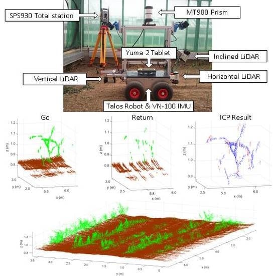
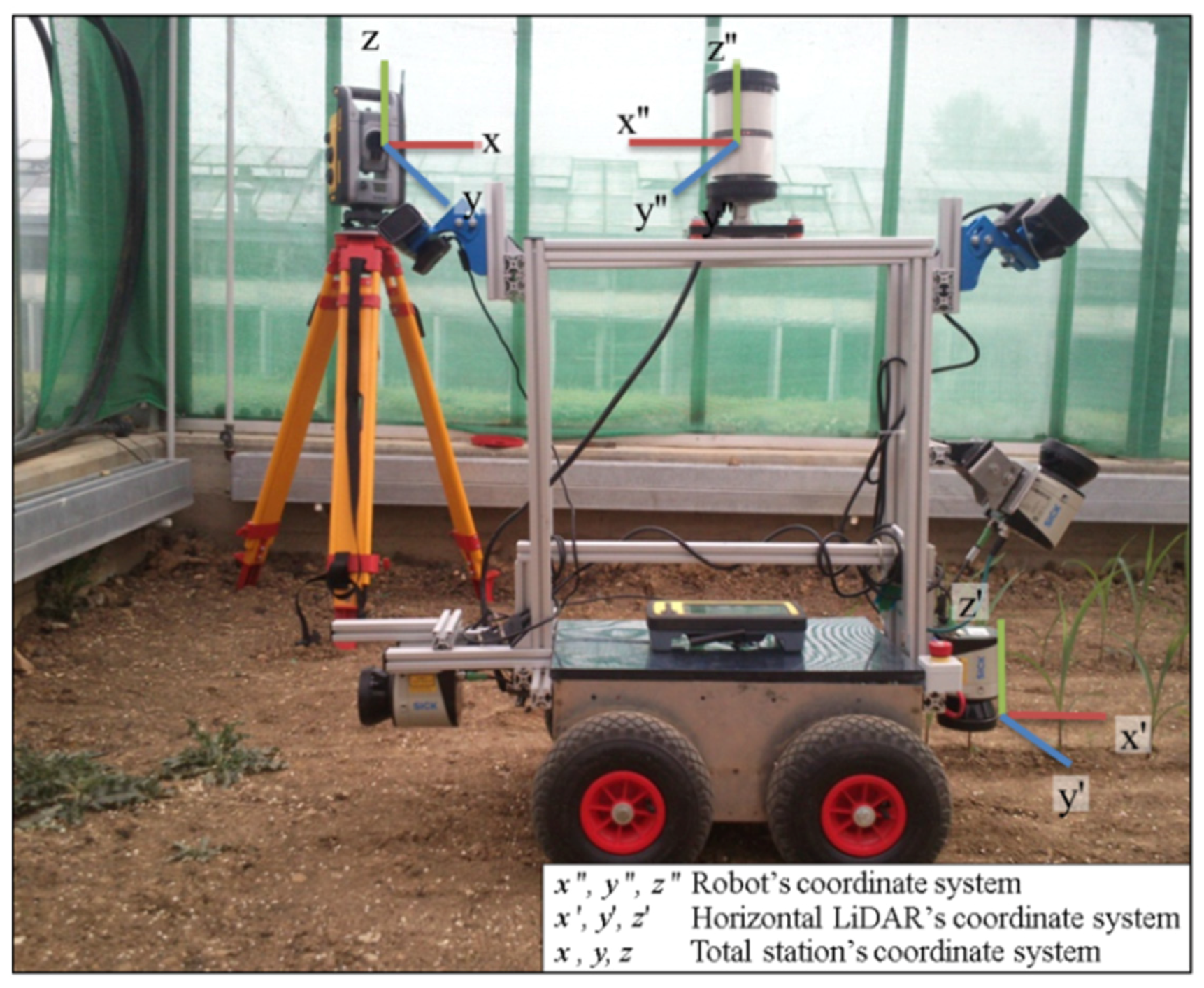
A small four-wheel autonomous robot called “Talos”, developed at the University of Hohenheim, was used to move the sensors between the maize crop rows. On this robot, different sensors were installed (see Figure 1): three LiDARs, an inertial measurement unit (IMU), and a prism which was tracked by a total station for georeferencing [26].
Figure 1. Equipment mounted on the “Talos” robot platform and the used total station.
Remotesensing 07 15870 g001
The model chosen for LiDAR sensors was the LMS 111 (SICK AG, Waldkirch, Germany). Its main characteristics are summarized in Table 1.
Table 1. LMS 111 technical data [27].
Functional DataGeneral Data
Operating range: from 0.5 m to 20 mLiDAR Class: 1 (IEC 60825-1)
Field of view/Scanning angle: 270°Enclosure Rating: IP 67
Scanning Frequency: 25 HzTemperature Range: −30 °C to +50 °C
Angular resolution: 0.5°Light source: Infrared (905 nm)
Systematic error: ±30 mmTotal weight: 1.1 kg
Statistical error: 12 mmLight spot size at optics cover/18 m: 8 mm/300 mm
Each LiDAR was installed with a different orientation and at a different location: horizontally, mounted at the front of the robot at a height of 0.2 m above the ground level; push-broom or inclined at an angle of 30°, mounted at the front of the robot at a height of 0.58 m; and vertically, mounted at the back of the robot at a height of 0.2 m (see Figure 1).
In all LiDAR sensors, two digital filters were activated for optimizing the measured distance values: a fog filter (becoming less sensitive in the near range (up to approx. 4 m); and a N-pulse-to-1-pulse filter, which filters out the first reflected pulse in case that two pulses are reflected by two objects during a measurement [27].
To acquire the three dimensional orientation of the robot in space during the field experiments, a VN-100 IMU (VectorNav, Dallas, TX, USA) was placed at the center of the robot. The accuracy values of the sensor were 2.0° RMS for the heading at static and dynamic mode, and 0.5° RMS and 1.0° RMS for both pitch and roll in static and dynamic mode, respectively.
In order to georeference the acquired LiDAR data, a SPS930 Universal Total Station was used (Trimble, Sunnyvale, CA, USA), with a distance measurement accuracy in tracking prism mode of ± (4 mm + 2 ppm). For that tracking mode, a Trimble MT900 Machine Target Prism was mounted on top of the robot, at the same axis as the IMU, and at a height of 1.07 m to always guarantee line of sight to the total station (see Figure 1). To ensure that all heights measured by the total station were positive, the software of the Total Station was configured in a way that the device had a height of 2 m above the ground, when in reality it was located only 1.2 m above the ground. The total station data was sent to a Yuma 2 rugged tablet computer (Trimble, Sunnyvale, CA, USA), which was connected to the robot computer via a serial RS232 interface for continuous data exchange. Five fixed control ground points were used for setting up the total station. In the specific setup the total station position was chosen as the origin of the coordinate system. If a predefined geodetic coordinate reference system (e.g., WGS84) is desired, the absolute coordinates of the fixed ground points are measured and are given as parameters during the total station set up. This variation does not affect the presented methodology.
Sensor acquisition and recording was accomplished by an embedded computer, equipped with an i3-Quadcore 3.3 GHz processor, 4 GB RAM and SSD hard drive. The robot computer ran on Linux (Ubuntu 14.04) and used the Robot Operating System (ROS-Indigo) middleware. The communications between the sensors and the robot computer were performed via RS232 interface for the IMU and Yuma 2; and via Ethernet for the LiDARs. All sensor data were time-stamped, according to the computer system time, and individually saved, respecting their acquisition frequencies: 25, 15, and 40 Hz for the LiDAR, total station, and IMU, respectively.

2.2. Field Experiments

Five rows of maize were seeded in a greenhouse to be independent of weather conditions. The row length was 5.2 m, while the width was defined as usual in maize to 0.75 m, with 41 plants per row. A theoretical distance between plants of 0.13 m was considered. The five rows were seeded with a standard deviation of 0.019, 0.017, 0.006, 0.048, and 0.047 m, respectively (see Figure 2), as is usually the result of seeding machines.
Data acquisition was performed when the crop was, mostly, at V3 leaf stage (by leaf collar method [28]), with an average height of 0.25 m. The robot movement was driven by a remote joystick, automatically adjusting the speed, at every path (between the cultivation lines) and direction (go and return) (see Figure 2), resulting in a total of eight recorded datasets. The average speed was around 0.06 m/s in order to acquire a high data density.
Figure 2. Representation of the total station location (*), the directions travelled by the robot during data acquisition, and the plant positions of the five maize rows (∙).
Remotesensing 07 15870 g002

2.3. Data Processing

This section explains the proposed methodology for getting the aerial point clouds of the maize crop rows referenced to the total station coordinates. This is a necessary prerequisite to perform the georeferenced overlapping of the aerial crop point clouds. For this purpose, it was necessary to conduct a pre-processing of the data, which was followed by a number of transformations and translations: (1) from the total station to the LiDAR sensor; and (2) from the LiDAR sensor to the scanned point. This process was repeated for each LiDAR, taking into account its location on the frame of the robot and its orientation.

2.3.1. Pre-Processing Data

Data pre-processing was performed, at each sensor used, in a different way. For this study, an off-line Matlab R2015a (MathWorks, Natick, MA, USA) process was used with actual field data collected during the field experiments.
The first step for the IMU data was to adapt the sensor coordinate system, depending on robot direction. Once the coordinate system was adjusted, a Savitzky-Golay FIR (Finite-Impulse Response) smoothing filter was applied, also known as polynomial smoothing or least-squares smoothing filter. This type of filter can preserve the high-frequency content of the desired signal, at the expense of not removing as much noise as the FIR averager [29]. The filter parameters were a polynomial order of seven and a frame size of 51.
Regarding total station’s data, the timestamp was adjusted given its latency over radio (40 ms), specified at the sensor technical data sheet [30].
In the case of the LiDARs sensors, the data was filtered to eliminate false positives or all those that did not contribute relevant information, considering only those detections with a distance between 0.03 m and 10 m, and with a remission value (reflectance percentage values from the laser pulse intensity) between 200 and 1000. Later, the resulting detections were transformed from polar to Cartesian coordinates, using the horizontal LiDAR coordinate system as a reference. The actual orientation of each LiDAR was considered during the subsequent applied transformations.
Data analysis was performed as long as information from all three sensors (total station, IMU, and LiDAR) was available. This could be justified by the sensor’s timestamp. Lastly, at every dataset, IMU and total station data were interpolated by the Piecewise Cubic Hermite Interpolating Polynomial (PCHIP) method [31], to each LiDAR data timestamp.

2.3.2. Serial Transformations and Translations

From Total Station to LiDAR Sensor

Due to the robot rigid body aluminium frame that was carrying the sensors, a static transformation and translation was performed, from the prism—tracked by the total station—to each LiDAR sensor. Thus, the relative coordinates (referred to the total station’s coordinate system) of each LiDAR and for each timestamp was obtained. For that, three steps were followed (see Figure 3 and Figure 4):
  • Firstly, the LiDARs’ coordinates at the robot's coordinate system ( x L i D A R , y L i D A R , z L i D A R ) were obtained, taking into account the prism as the origin, following the rigid translation (see Equation (1)) values of each LiDAR (see translation values at Table 2).
    [ x L i D A R y L i D A R z L i D A R ] = [ x _ t r a n s l a t i o n y _ t r a n s l a t i o n p r i s m _ h e i g h t + z _ t r a n s l a t i o n ]
  • Secondly, a transformation for evaluating the three dimensional orientation of the robot was applied at the coordinates obtained for each LiDAR (see Equation (2)). For that, the IMU values (roll “φ”, pitch “θ”, and yaw “ψ”) were considered at the LiDAR’s timestamp “t” ( x φ t , y θ t , z ψ t ) .
  • Finally, a second translation was performed (see Equation (2)) from the prism-tracked coordinates to the total station for that specific timestamp ( x p r i s m t , y p r i s m t , z p r i s m t ) . Thus, the LiDAR coordinates at the total station’s coordinate system for the evaluated time ( x L i D A R t , y L i D A R t , z L i D A R t ) were obtained.
    [ x L i D A R t y L i D A R t z L i D A R t 1 ] = [ x L i D A R y L i D A R z L i D A R 1 ] × [ 1 0 0 0 0 cos ( x φ t ) sin ( x φ t ) 0 0 sin ( x φ t ) cos ( x φ t ) 0 0 0 0 1 ] × [ cos ( y θ t ) 0 sin ( y θ t ) 0 0 1 0 0 sin ( y θ t ) 0 cos ( y θ t ) 0 0 0 0 1 ] ×                         [ cos ( z ψ t ) sin ( z ψ t ) 0 0 sin ( z ψ t ) cos ( z ψ t ) 0 0 0 0 1 0 0 0 0 1 ] × [ 1 0 0 0 0 1 0 0 0 0 1 0 x p r i s m t y p r i s m t z p r i s m t 1 ]

From LiDAR Sensor to Scanned Point

Once the LiDAR sensor’s coordinates at the total station’s coordinates system at the evaluated timestamp “t” were obtained, the next step was to convert the local LiDAR point cloud, for that time, into total station’s coordinates system. For that, four steps were followed (see Figure 3 and Figure 4):
  • The starting points were the Cartesian coordinates obtained at every LiDAR scan, using the horizontal orientation as reference, for the evaluated time ( x point t , y point t , z point t ) .
  • In order to integrate the LiDAR’s scan into the robot’s coordinate system, a different transformation ( x φ , y θ , z ψ ) was applied (see Equation (3)) depending on the LiDAR’s orientation and the robot’s direction (see Table 2). Table 2 presents the first rough calibration of the LiDAR’s positions and orientations. This was performed using a measuring tape and a bullseye level for the two-dimensional plane levelling (roll and pitch angles). An angle meter was used for precise measurement of the inclined LiDAR slope. The thorough calibrations were performed later on during the implementation of the ICP algorithm at the point cloud overlapping.
    [ x point t y point t z point t 1 ] = [ x point t y point t z point t 1 ] × [ 1 0 0 0 0 cos ( x φ ) sin ( x φ ) 0 0 sin ( x φ ) cos ( x φ ) 0 0 0 0 1 ] × [ cos ( y θ ) 0 sin ( y θ ) 0 0 1 0 0 sin ( y θ ) 0 cos ( y θ ) 0 0 0 0 1 ] ×                                                  [ cos ( z ψ ) sin ( z ψ ) 0 0 sin ( z ψ ) cos ( z ψ ) 0 0 0 0 1 0 0 0 0 1 ]
Table 2. Transformation and translation values depending on LiDAR’s orientation and robot direction.
LiDAR OrientationDirectionRoll x φ (°)Pitch y θ (°)Yaw z ψ (°)x Translation (m)y Translation (m)z Translation (m)
Horizontal Go0−1800−0.4500.205
Return180000.4500.205
Inclined Go0−30180−0.5100.58
Return0−3000.5100.58
Vertical Go0−9000.5726−0.01770.1997
Return180−900−0.57260.01770.1997
3.
Then, a second transformation to evaluate the three dimensional orientation of the robot was applied at LiDAR’s scan (see Equation (4)). For that, the IMU values (roll “φ”, pitch “θ”, and yaw “ψ”) were considered at timestamp “t” ( x φ t , y θ t , z ψ t ) .
4.
Finally, a translation from the LiDAR coordinates to the total station’s coordinate system for the evaluated time “t” ( x L i D A R t , y L i D A R t , z L i D A R t ) was performed (see Equation (4)); thereby each LiDAR scanned point at the total station's coordinate system ( x point t , y point t , z point t ) was obtained.
[ x point t y point t z point t 1 ] = [ x point t y point t z point t 1 ] × [ 1 0 0 0 0 cos ( x φ t ) sin ( x φ t ) 0 0 sin ( x φ t ) cos ( x φ t ) 0 0 0 0 1 ] × [ cos ( y θ t ) 0 sin ( y θ t ) 0 0 1 0 0 sin ( y θ t ) 0 cos ( y θ t ) 0 0 0 0 1 ] ×                         [ cos ( z ψ t ) sin ( z ψ t ) 0 0 sin ( z ψ t ) cos ( z ψ t ) 0 0 0 0 1 0 0 0 0 1 ] × [ 1 0 0 0 0 1 0 0 0 0 1 0 x L i D A R t y L i D A R t z L i D A R t 1 ]
In Figure 3 the robot, LiDAR, and total station coordinate system are depicted, while Figure 4 presents an example of the whole transformation process for the vertical LiDAR orientation.
Figure 3. Robot’s (double quote), LiDAR’s (single quote), and total station’s (unquoted) coordinate systems.
Remotesensing 07 15870 g003
Figure 4. (Left) Transformation and translation process from total station to the LiDAR, and (Right) from the LiDAR to the scanned point. Double quoted, single quoted, and unquoted correspond to the robot’s, LiDAR’s, and total station’s coordinate system, respectively.
Remotesensing 07 15870 g004

2.4. Point Cloud Overlapping

For developing the proposed methodology (i.e., georeferenced overlapping of point clouds for three-dimensional maize plant reconstruction), each LiDAR orientation processed data was evaluated individually (see Figure 5). Thus, considering the goal of this research, it was possible to determine which configurations were satisfactory.
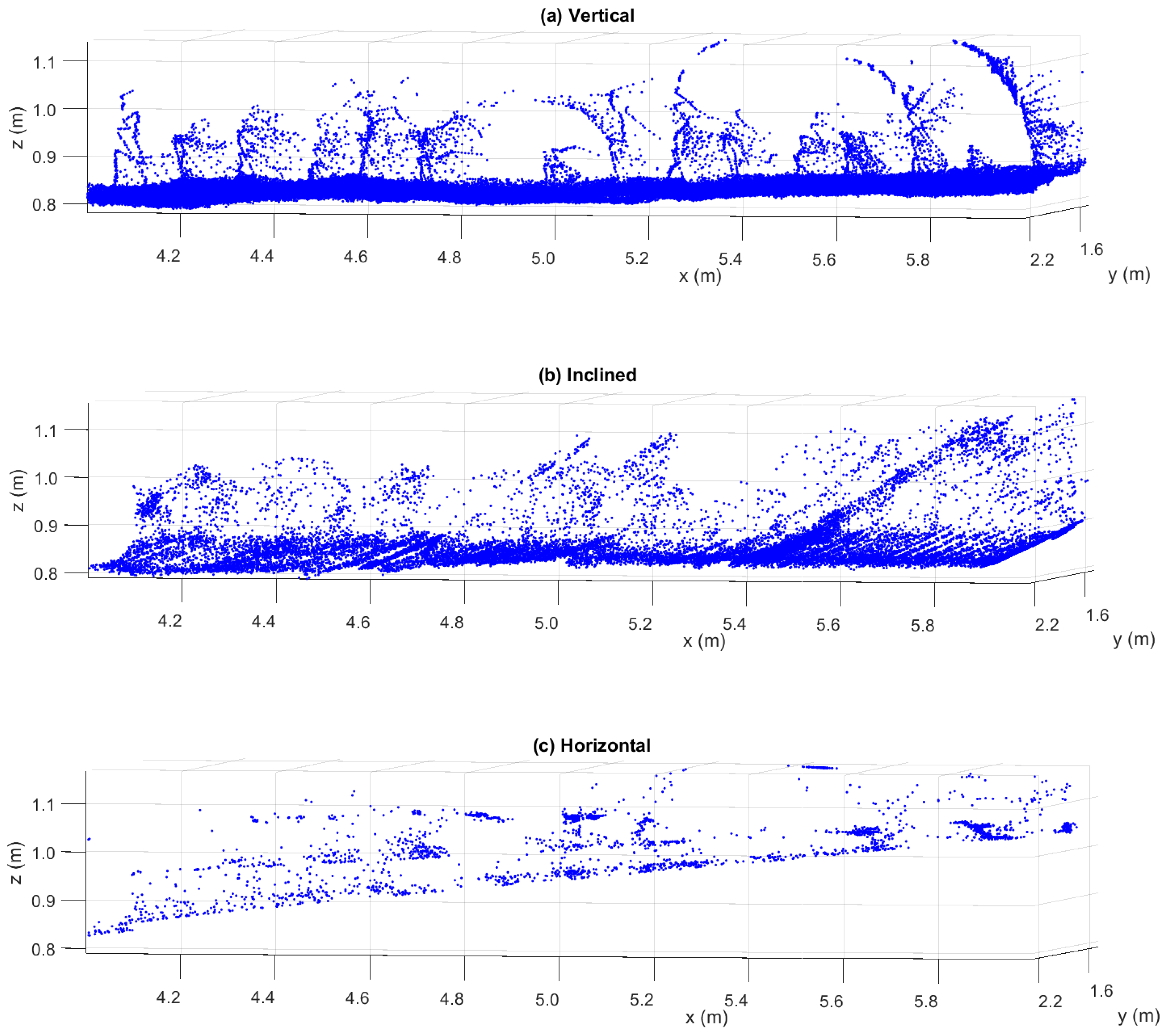
Surroundings characterization by the horizontal LiDAR’s orientation was directly related to ground unevenness as its scanned points were at a larger distance compared to the other two LiDARs. In case of a leveled surface, only a small part of the plant will be detected by obtaining a single cross section for each plant at the corresponding LiDAR height. The soil will not be detected, thereby hampering the procedure of noise removal. If the robot suffers fluctuations or moves on a sloping ground (e.g., a small downslope suffered by the “Talos” robot, see Figure 5c), a greater number of incorrect plant detections would be obtained (not just at the LiDAR height), making possible the ground detection in a higher distance as LiDAR and ground plane are not parallel. In this way, a horizontal LiDAR’s orientation could be useful for row navigation of an autonomous vehicle, but not for plant reconstruction, as the plant detections are limited. Thus, its use was discarded for the purpose of the present study, which was based on the vertical and inclined LiDAR’s orientations.
To do the evaluations of the aerial point clouds (of the selected LiDAR’s orientation: vertical and inclined), in addition to their shapes and resolutions, it was also important to evaluate the outlier effect obtained at each orientation. According to a previous study: “An outlier is an observation that deviates so much from other observations. It can be caused by different sources and they are mainly measurements that do not belong to the local neighborhood and do not obey the local surface geometry” [32].
This effect is enhanced when smaller objects than the footprint of the laser beam are detected. In these cases, instead of registering a clear detection, in which the entire beam hits the object, the reflected pulse received at the LiDAR will belong partially (depending on the shutter percentage) to the desired object, as well as to the unwished second target, which is behind the first one.
Figure 5. 
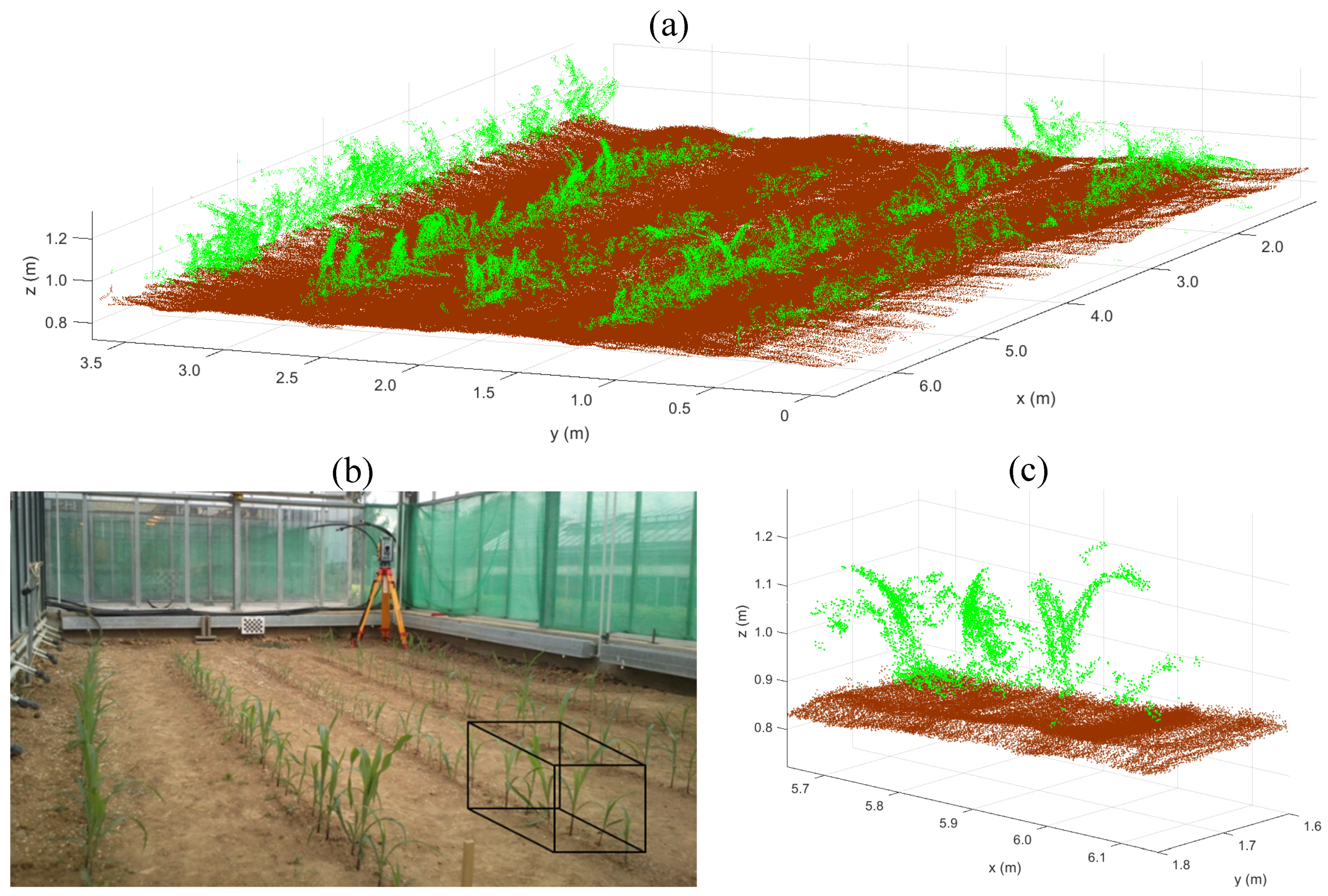
Raw data point cloud obtained with (a) vertical; (b) inclined; and (c) horizontal LiDAR orientation while “Talos” was moving in descending order in x-axis.
Remotesensing 07 15870 g005
In this regard, Sanz-Cortiella et al. in [33] evaluated the effect of partial blockages of the beam on the distance measured by the LiDAR, deducting that distance value depends more on the blocked radiant power than on the blocked surface area of the beam, and that there was an area of influence which was dependent on the shutter percentage. In their case, this varied from 1.5 to 2.5 m with respect to the foreground target, so if the second impact of the laser beam occurred within that range it would affect the measurement given by the sensor. However, when the second target was outside this area of influence, the sensor ignored this second target and gave the distance to the first impact target. Thereby, its understanding was an essential process before the point clouds overlapping, adjusting the noise removal filter to their need.
Vertical LiDAR’s orientation provided basically the plant projection. Its resolution was greatly affected by the robot’s speed. Consequently, keeping the speed constant (automatically) was of great importance. On the other hand, the inclined LiDAR’s orientation had a wider field of view, and the plants were detected more than once by different beam angles and at different times. Due to this inclined orientation, the robot’s speed was not that crucial as it was for the vertical orientation. For the inclined LiDAR, the ground roughness was highly important, as the detections were performed at a larger distance. Therefore, small precision flaws during the transformations would affect, to a greater extent, the point cloud’s precision (see Figure 5).
Regarding the outlier effect, cumulative observations were detected from the vertical LiDAR’s orientation. These detections were mainly at the back side of the plant in respect to the LiDAR view, in line with the projection angle of the scan. The outlier shape remained constant as the plants were scanned just once. On the other hand, the outlier shape which was obtained from the inclined LiDAR’s orientation was not constant. In this case, each plant was detected at different scan angle and at different time, requiring a more exhaustive filtering (see Figure 5).
The 3D point cloud overlapping was performed at each path and crop line using both go and return robot's travelling direction. Thus, by manual distance delimitation, four different 3D point clouds were used for each row: vertical and inclined go and return.
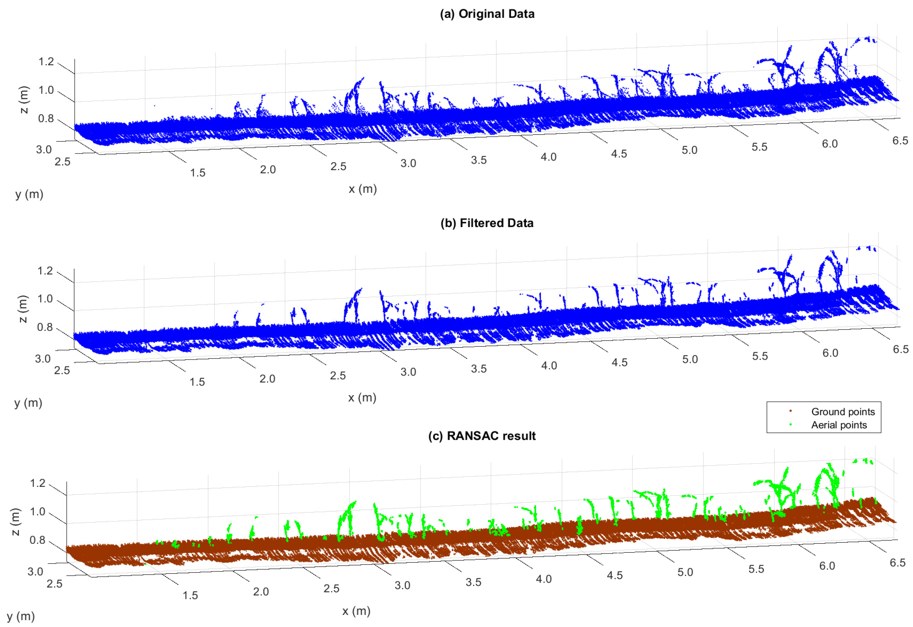
The aerial point data cloud was extracted by a succession of pre-filters. In the first place, all the points which did not provide new information were removed using a gridding filter, thus reducing the size of the point cloud. Then, the point cloud noise was reduced by a sparse outlier removal filter [34], making the application of the RANSAC algorithm easier, in order to distinguish the aerial from the ground points. The applied pre-filters were:
  • Gridding filter: returns a down sampled point cloud using box grid filter. GridStep specifies the size of a 3D box. Points within the same box are merged to a single point in the output (see Table 3).
  • Noise Removal filter: returns a filtered point cloud that removes outliers. A point is considered to be an outlier if the average distance to its K nearest neighbors is above a threshold [34] (see Table 3). In the case of the inclined LiDAR’s orientation it was necessary to apply serially, as mentioned earlier, a second noise removal filter.
  • RANSAC fit plane: this function, developed by Peter Kovesi [35], uses the RANSAC algorithm to robustly fit a plane. It only requires the selection of the distance threshold value between a data point and the defined plane to decide whether a point is an inlier or not. For plane detection, which was the same as ground detection in our case, the evaluations were conducted at every defined evaluation interval or vehicle advance (see Table 3).
Table 3. Point clouds overlapping parameters.
LiDAR Orient.GridStep (m3)Noise Removal Filter INoise Removal IIRANSAC
NeighborsStd. thresholdNeighborsStd. thresholdEval. Intervals (m)Threshold (m)
Vertical(3 × 3 × 3) × 10−9101--0.1950.07
Inclined50.3101
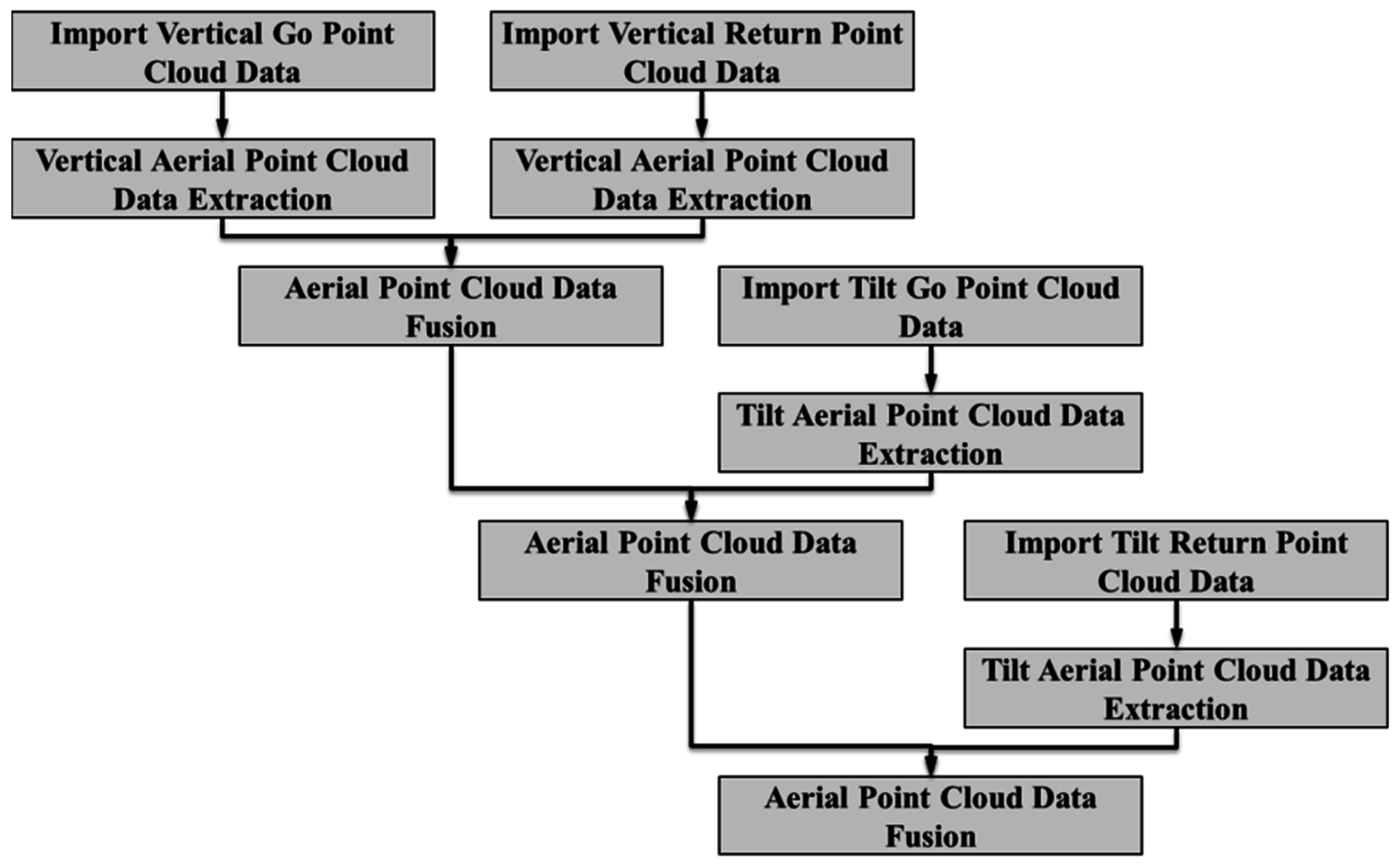
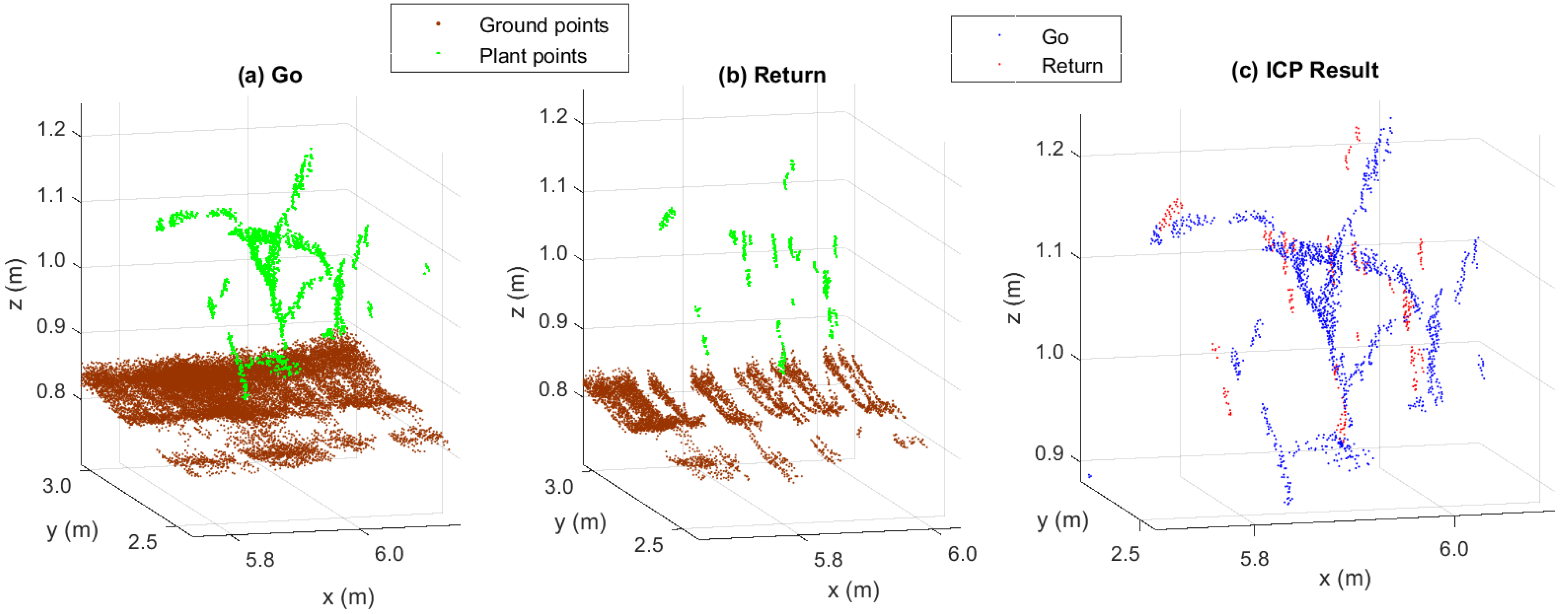
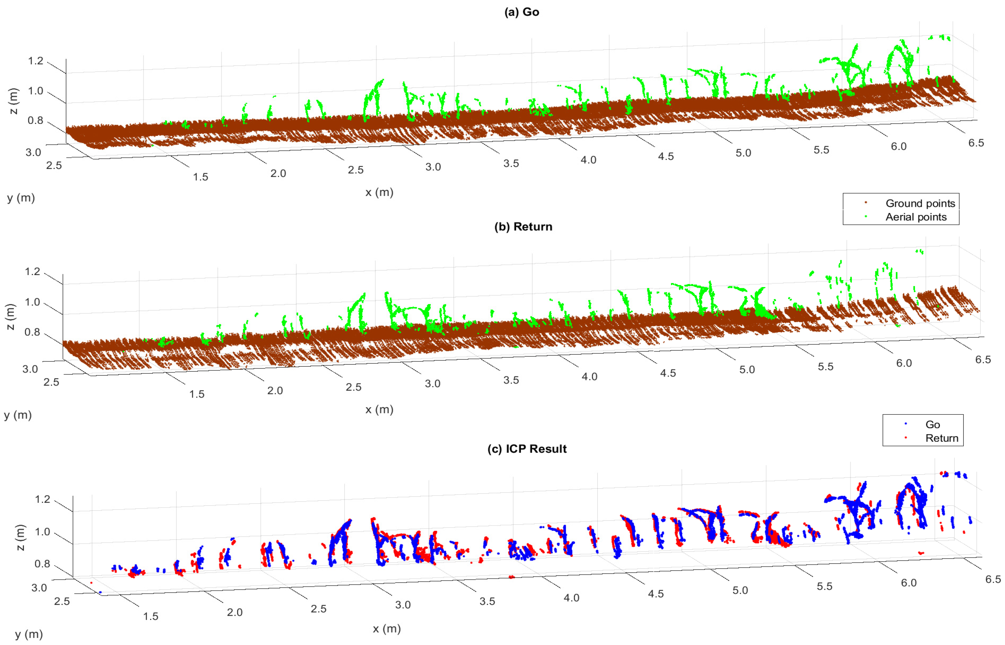
To perform the point cloud data overlapping, considering only the resulting aerial points from the previous process, serial fusions were performed. Firstly, the aerial vertical point clouds (go and return) were fused, followed by the aerial inclined point cloud when the robot goes, and finally by the aerial inclined point cloud when the robot returns (see Figure 6). The required steps for point cloud fusion were:
4.
Iterative Closest Point (ICP): the ICP algorithm takes two point clouds as an input and returns the rigid transformation (rotation matrix R and translation vector T) that best aligns the new point cloud to the previous referenced point cloud. It is using the least squares minimization criterion [36]. The starting referenced point cloud was the one obtained by the vertical LiDAR’s orientation when going.
5.
Gridding filter: the same 3D box size was considered, as defined at the aerial point cloud extraction (see Table 3).
Figure 6. Overlapping process followed at each path and row.
Remotesensing 07 15870 g006
Table 3 shows the parameter values that were chosen during the point clouds overlapping. In order to achieve a fine resolution or detailed characterization of the plant impacts during the point’s merge process, a box grid filter length of 3 mm was selected. For ground removal, the RANSAC algorithm was performed within a factor of 1.5 of the theoretical distance between the plants, thus ensuring its adaptation to ground relief and the presence of maize plants at each interval, and not only ground detections that would result in a malfunction of the algorithm. For ensuring complete ground detection, the distance threshold was set 3.5 times higher than the statistical LiDAR error.
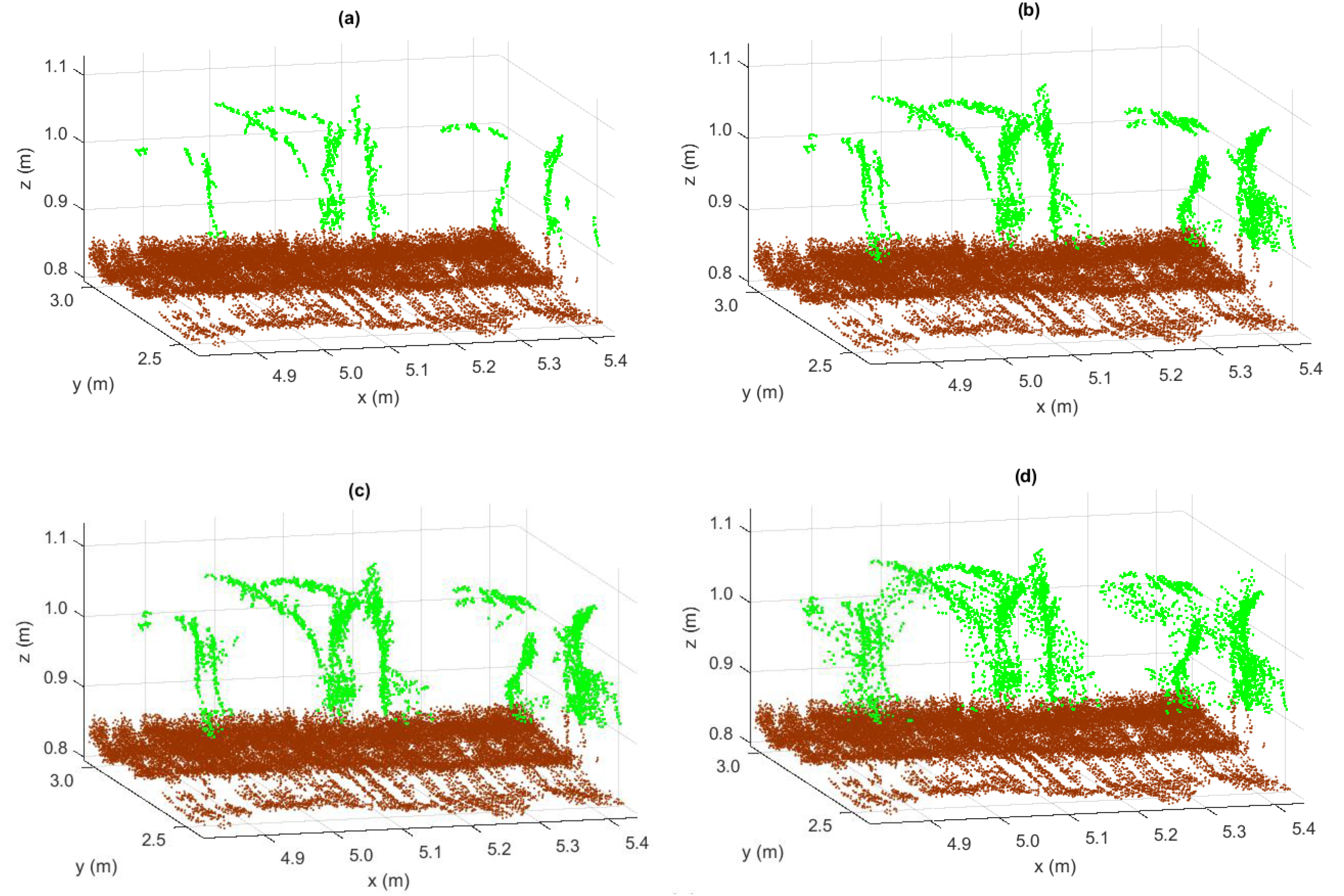
Regarding noise removal filter parameters, nearest neighbor points were used to adjust the sensitivity of the filter to noise. By decreasing the value of nearest neighbor points a more sensitive filter was obtained. On the other hand, the outlier threshold set the standard deviation from the mean of the average distance to neighbors of all points, to assess whether the point is an outlier or not. By increasing the value of outlier threshold a more sensitive filter was obtained. A neighbor point’s parameter was evaluated by keeping constant the outlier threshold to its default value equal to one. This was accomplished by trial and error, selecting those filter values that better reduce the point cloud noise without losing much useful information.
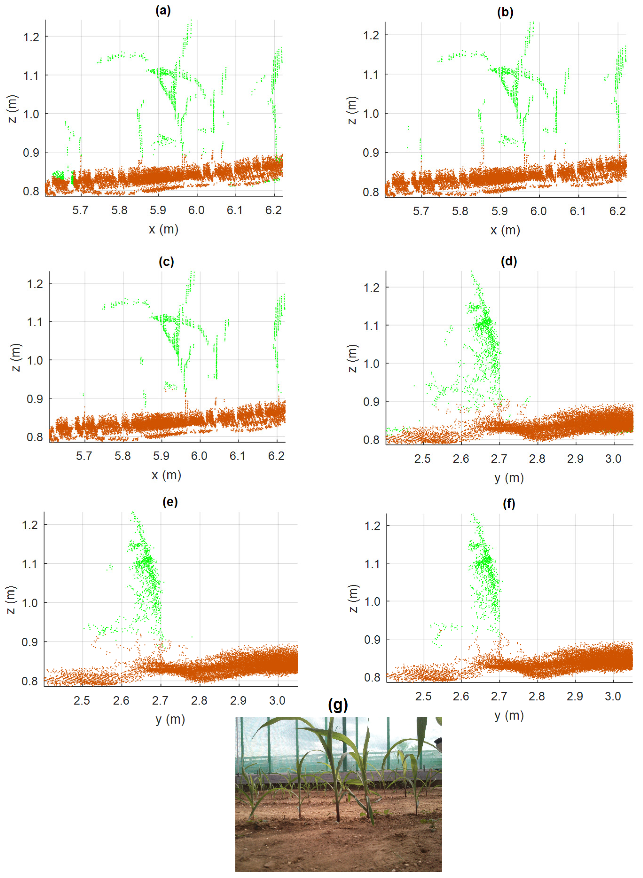
Figure 7 presents the front (XZ) and lateral (YZ) view during vertical orientation noise removal filter evaluation for five, 10, and 20 of nearest neighbor points. Figure 7 shows how, by increasing the number of considered neighbors, a greater number of outliers were removed, but eliminating at the same time useful information (see the removed maize at the left side in Figure 7c). At the vertical orientation the number of neighbors was configured to a value of 10. On the other hand, the inclined orientation, with a more dispersed but less dense point cloud, needed the inclusion of a previous noise removal filter. For this filter the same approach as at the vertical orientation was followed.
Figure 7. 
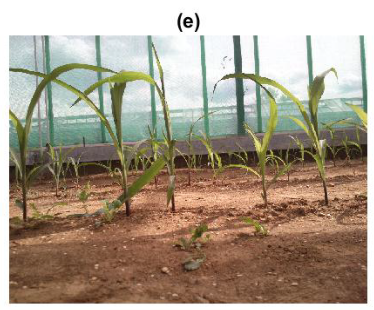
Plants reconstruction during vertical orientation noise removal filter evaluation. (ac) XZ view considering five, 10, and 20 nearest neighbor points. (df) YZ view considering five, 10, and 20 nearest neighbor points. (g) Image of the front view of the plants.
Remotesensing 07 15870 g007

3. Results and Discussion

Table 4 presents the raw point cloud data obtained during the experiment. An initial manual delimitation was performed based on row dimensions. As the greenhouse terrain was mostly flat, a low number of detections were acquired by the horizontal LiDAR, representing only the 6.5% of the total detections. On the opposite side, almost two-thirds (65.8%) of the raw detections were acquired by the vertical LiDAR. The inclined LiDAR contributed 27.7%. Clearly, for each row direction (go or return) the sum of points for all three LiDARs (vertical, inclined, and horizontal) is 100%.
As it was mentioned in the previous section, horizontal LiDAR information was discarded. This decision was taken, in addition to its reduced contribution, due to the non-viable implementation of the proposed methodology on its point cloud pattern, as ground detection was required by the RANSAC fit plane function.
Table 5 shows the point cloud reduction of the vertical and inclined LiDAR data during the filtering process and the aerial point cloud extraction.
Table 4. Raw point cloud data recorded during the experiments.
GoReturn
RowVerticalInclinedHorizontalVerticalInclinedHorizontal
1147,839 (67.8%)52,267 (24.0%)17,788 (8.2%)230,918 (72.6%)61,832 (19.4%)25,453 (8.0%)
2135,406 (67.2%)52,069 (25.8%)14,107 (7%)118,372 (66.3%)49,799 (27.9%)10,503 (5.9%)
3176,956 (68.4%)74,659 (28.9%)6928 (2.7%)122,287 (63.3%)62,085 (32.1%)8894 (4.6%)
4182,801 (63.6%)83,829 (29.2%)20,891 (7.3%)110,882 (64.4%)49,799 (28.9%)11,568 (6.7%)
596,887 (61.3%)46,535 (29.4%)14,703 (9.3%)121,867 (58.3%)74,329 (35.5%)12,969 (6.2%)
Table 5. Point cloud reduction during aerial point cloud extraction.
LiDARDirectionRowRaw DataGriddingNoise RemovalAerial Points
VerticalGo1147,839 (100%)138,832 (93.9%)133,035 (90.0%)3392 (2.3%)
2135,406 (100%)129,824 (95.9%)124,515 (92.0%)3667 (2.7%)
3176,956 (100%)152,789 (86.3%)147,981 (83.6%)1765 (1.0%)
4182,801 (100%)158,960 (87.0%)153,960 (84.2%)3615 (2.0%)
596,887 (100%)93,892 (96.9%)90,659 (93.6%)1739 (1.8%)
Return1230,918 (100%)187,909 (81.4%)182,355 (79.0%)4466 (1.9%)
2118,372 (100%)100,197 (84.6%)95,605 (80.8%)3333 (2.8%)
3122,287 (100%)115,917 (94.8%)111,752 (91.4%)1786 (1.5%)
4110,882 (100%)107,510 (97.0%)103,605 (93.4%)3153 (2.8%)
5121,867 (100%)102,549 (84.1%)98,623 (80.9%)2086 (1.7%)
InclinedGo152,267 (100%)41,913 (80.2%)33,965 (65.0%)3808 (7.3%)
252,069 (100%)48,364 (92.9%)39,149 (75.2%)2418 (4.6%)
374,659 (100%)64,623 (86.6%)52,327 (70.1%)1052 (1.4%)
483,829 (100%)65,919 (78.6%)55,350 (66.0%)3259 (3.9%)
546,535 (100%)42,868 (92.1%)35,045 (75.3%)1274 (2.7%)
Return161,832 (100%)57,381 (92.8%)46,914 (75.9%)3845 (6.2%)
249,799 (100%)46,843 (94.1%)38,192 (76.7%)4593 (9.2%)
362,085 (100%)56,734 (91.4%)46,328 (74.6%)2123 (3.4%)
460,891 (100%)58,000 (95.3%)48,954 (80.4%)2925 (4.8%)
574,329 (100%)58,928 (79.3%)48,663 (65.5%)1846 (2.5%)
Total 2,062,510 (100%)1,829,952 (88.7%)1,686,977 (81.8%)56,145 (2.7%)
As an example, considering the point cloud obtained by the vertical LiDAR’s orientation when the robot was going for the path 1 and row 2, Figure 8 shows the results at each aerial point cloud extraction process step. While the original point cloud consisted of 135,406 scan detections, they were reduced by 4.1% and 3.9% once the grid and noise removal filters were applied, respectively.
In the filtered point cloud, the RANSAC algorithm was used. This made possible to divide the ground detections, defined by the fit plane, from the aerial detections (represented by brown and green at the Figure 8c). The aerial point cloud was always represented by a small part (<10%) of the recorded detections at the original point cloud. This percentage was depended on the used LiDAR orientation (2.7% for our example). This low percentage of points under consideration facilitated the processing time of the subsequent steps, increasing at the same time the accuracy of the ICP algorithm.
The inclined LiDAR raw data were almost three times less than compared with the raw data of the vertical LiDAR (see Table 4). This difference in number of points disappears when the aerial points outcome is considered solely, where an equal percentage was contributed by each LiDAR orientation (vertical and inclined) (see Table 5). This could be explained by considering that plants are detected more than once by the inclined LiDAR, while this detection is performed only once by the vertical LiDAR.
Figure 8. (a) Original point cloud; (b) filtered point cloud; and (c) RANSAC results during aerial point cloud extraction for the vertical LiDAR’s orientation when going at path 1 and row 2.
Remotesensing 07 15870 g008
Continuing with the same example, Figure 9 shows the point cloud result during aerial point cloud fusion by the vertical LiDAR’s orientation when the robot was going and returning for the path 1 and row 2. The ICP algorithm was applied as soon as the aerial points were defined. The number of detections for going and returning that corresponding to aerial points were 3667 and 3333, respectively (see Table 6). Equation (5) set out the rigid transformation results (Euler angles R in degrees and translation vector T “XYZ” in m) that best align the vertical returning point cloud to the vertical going point cloud. Similarly, Equation (6) sets out the average rigid transformation obtained after all fusions during the experiment. Figure 9c presents the resulting point cloud fusion, after applying the rigid ICP transformation. Figure 10 shows a zoom in plants presented at Figure 9, in order to provide a better felling of the agreement between the different point clouds.
R = [ 0.11 0.11 0.86 ] ,   T = [ 0.11 0.01 0.02 ]
R = [ 0 ± 0.81 0 ± 0.41 2.31 ± 11.33 ] , T = [ 0.05 ± 0.05 0.06 ± 0.16 0.02 ± 0.23 ]
Figure 9. (a) RANSAC go results; (b) RANSAC return results; and (c) ICP result of the aerial point clouds for the vertical LiDAR’s orientation when going and returning at path 1 and row 2.
Remotesensing 07 15870 g009
Figure 10. (a) RANSAC go results; (b) RANSAC return results; and (c) ICP result of the aerial point clouds for the vertical LiDAR’s orientation when going and returning at path 1 and row 2 for a specific row interval.
Remotesensing 07 15870 g010
On Table 6 the first column on the right is the total amount of aerial points for each row and for the entire experiment. As it can be seen the total amount of aerial points was 55,083 (100%). The obtained values expose that 51.9% of the final aerial points were provided by the vertical LiDAR. The rest 48.1% was provided by the inclined LiDAR. In Table 6 the percentage for each LiDAR, the going and returning are also presented.
Table 6. Aerial point cloud provided during the data fusion (V:vertical LiDAR orientation; I:inclined LiDAR orientation). The percentage of the contributed points of each step during the fusion process is also presented.
RowVGoVReturnVGo + VReturn “Grid”VGo + VReturn + IGo “Grid”VGo + VReturn + IGo + IReturn “Grid”
13392 (22.4%)4466 (29.4%)7711 (50.8%)11,391 (75.1%)15,173 (100%)
23667 (26.6%)3333 (24.2%)6915 (50.2%)9297 (67.5%)13,775 (100%)
31765 (26.8%)1786 (27.1%)3491 (53.0%)4500 (68.3%)6591 (100%)
43615 (28.5%)3153 (24.8%)6684 (52.6%)9820 (77.3%)12,705 (100%)
51739 (25.4%)2086 (30.5%)3809 (55.7%)5072 (74.2%)6839 (100%)
Total14,178 (25.7%)14,824 (26.9%)28,610 (51.9%)40,080 (72.8%)55,083 (100%)
As new point clouds were overlapping, provided by different LiDAR’s orientation (vertical and inclined) and time instances (go and return), a more realistic 3D reconstruction was obtained. Through the serial inclusion of the four views (vertical go (Figure 11a), plus vertical return (Figure 11b), plus inclined go (Figure 11c), and plus inclined return (Figure 11d)), additional scanning data were provided. Taking into account only one LiDAR single-view, not all aerial points which define a plant were considered. Through the incorporation of new LiDAR views, these aerial points’s exclusion is reduced. By this inclusion process, different points of view of the scene were taken into account, resulting in a more realistic representation of the surrounding area. There is a point where extra information, by the inclusion of a new LiDAR view, may introduce noise to the fused point cloud. In this way, the inclusion of different LiDAR views should be carefully examined, as it may not only incorporate new useful information but also noise (see Figure 11d).
Figure 11. Detail of the aerial point cloud provided during the data fusion process at path 1 and row 2. (a) Vertical Go; (b) Vertical Go + Return; (c) Vertical + Inclined Go; (d) Vertical + Inclined; and (e) actual plants.
Remotesensing 07 15870 g011aRemotesensing 07 15870 g011b
Figure 12 shows the final point cloud once the georeferenced overlapping process of the eight trips was completed (go and return at every path), allowing the visualization of the five maize rows on which the entire experiment was performed. A low number of aerial points detected at the end of row three can be seen (background of the middle row according to the figure). This highlights the seedling emergence problems that these plants had. Figure 12 also shows a greater outlier effect at the first maize row (y-axis coordinates from 3.0 to 3.6 m). The wall that delimited the greenhouse was very close to this row (about one meter) causing a second impact of the laser beam within the area of influence and thereby affecting the measurement given by the sensor.
Figure 12. (a) 3D view of the 21 m2 (3.75 m wide and 5.6 m length) of the maize field, with 1,630,832 and 55,083 ground and plant impacts, respectively; (b) Picture of the maize field; (c) Plants zoom of the area within the black cube represented in b.
Remotesensing 07 15870 g012

4. Conclusions

A new methodology for georeferenced 3D reconstruction of maize plant structure during the first stages of development has been proposed. This has been accomplished using a combination of a total station, an IMU, several LiDAR point clouds with different angles and timestamps provided by a moving on autonomous vehicle, and a complex multistep algorithm for data processing. For point cloud overlapping, a filtering process was conducted in order to down sample the data by merging, removing the noise, and obtaining the aerial points once the ground was detected. The application of the ICP algorithm proved to be very important during point cloud fusion by finding the best translation and rotation matrices that minimize an error metric based on the distance between point clouds. Through its application, sensors and transformation errors (from total station, IMU, and LiDAR) were adjusted to the reference point cloud. From the results it was proved that the orientation of the LiDAR is important and specifically in relation to the number of final aerial points that are used for the 3D plant reconstruction.
The proposed methodology can help the aim of developing a georeferenced 3D plant reconstruction of an entire crop. The produced 3D plant structure can be used for plant phenotyping purposes in order to detect complex plant traits. Having a georeferenced 3D reconstruction of the crop from different growth stages, other time-stamped georeferenced data can be fused to the existing crop reconstruction. Finally, the use of the total station and the level of accuracy that this sensor provides to the final 3D crop reconstruction, can offer a big advantage when performing precision farming related applications. More specifically, it can help towards crop protection using autonomous machines or harvesting utilizing robotic systems.
In turn, the proposed methodology could be useful for other LiDAR data processing when plant and ground are detected (prerequisite for RANSAC’s application). This might be the case of point clouds acquired of other plants, crops, or trees, whether from a UGV (Unmanned Ground Vehicle) or from a UAV (Unmanned Aerial Vehicle), which allow the data collection from different inclination angles due to their high maneuverability.
For the purpose of conducting a method for verifying the aerial points obtained in this article, further work is required by comparing these results with the images recorded during the experiments by a Kinect (Microsoft, Washington, DC, USA), using its depth information and green channel.

Acknowledgments

The research leading to these results has received funding from the European Union’s Seventh Framework Programme (FP7/2007–2013) under Grant Agreement No. 245986, by a mobility grant of UPM and by the Madrid's community, S2013/ABI-2747 (TAVS-CM) and Structural Funds of the European Union.The project was conducted at the Max-Eyth Endowed Chair (Instrumentation & Test Engineering) at the Hohenheim University (Stuttgart, Germany) which is partly grant funded by the Deutsche Landwirtschafts-Gesellschaft e.V. (DLG).

Author Contributions

The first four authors conducted all of the in-person fieldwork from March until May 2015 supervised and guided by the fifth author. Once that the principal author finished his stay in the host university (University of Hohenheim) and returned to his home university (Technical University of Madrid), he conducted the data analysis as well as the wording of this article. Data were discussed and analyzed on multiple occasions by the first, second and last author. The final article was jointly authored.

Conflicts of Interest

The authors declare no conflict of interest.

References

  1. Omasa, K.; Hosoi, F.; Konishi, A. 3D LiDAR imaging for detecting and understanding plant responses and canopy structure. J. Exp. Bot. 2007, 58, 881–898. [Google Scholar] [CrossRef] [PubMed]
  2. Li, F.; Cohen, S.; Naor, A.; Shaozong, K.; Erez, A. Studies of canopy structure and water use of apple trees on three rootstocks. Agric. Water Manag. 2002, 55, 1–14. [Google Scholar] [CrossRef]
  3. Kjaer, K.H.; Ottosen, C.-O. 3D laser triangulation for plant phenotyping in challenging environments. Sensors 2015, 15, 13533–13547. [Google Scholar] [CrossRef] [PubMed]
  4. Li, L.; Zhang, Q.; Huang, D. A review of imaging techniques for plant phenotyping. Sensors 2014, 14, 20078–20111. [Google Scholar] [CrossRef] [PubMed]
  5. Ivanov, N.; Boissard, P.; Chapron, M.; Andrieu, B. Computer stereo plotting for 3-D reconstruction of a maize canopy. Agric. For. Meteorol. 1995, 75, 85–102. [Google Scholar] [CrossRef]
  6. De Moraes Frasson, R.P.; Krajewski, W.F. Three-dimensional digital model of a maize plant. Agric. For. Meteorol. 2010, 150, 478–488. [Google Scholar] [CrossRef]
  7. Nguyen, T.T.; Slaughter, D.C.; Max, N.; Maloof, J.N.; Sinha, N. Structured light-based 3D reconstruction system for plants. Sensors 2015, 15, 18587–18612. [Google Scholar] [CrossRef] [PubMed]
  8. Chaivivatrakul, S.; Tang, L.; Dailey, M.N.; Nakarmi, A.D. Automatic morphological trait characterization for corn plants via 3D holographic reconstruction. Comput. Electron. Agric. 2014, 109, 109–123. [Google Scholar] [CrossRef]
  9. Li, D.; Xu, L.; Tan, C.; Goodman, E.D.; Fu, D.; Xin, L. Digitization and visualization of greenhouse tomato plants in indoor environments. Sensors 2015, 15, 4019–4051. [Google Scholar] [CrossRef] [PubMed]
  10. Andújar, D.; Fernández-Quintanilla, C.; Dorado, J. Matching the best viewing angle in depth cameras for biomass estimation based on poplar seedling geometry. Sensors 2015, 15, 12999–13011. [Google Scholar] [CrossRef] [PubMed]
  11. Palleja, T.; Landers, A.J. Real time canopy density estimation using ultrasonic envelope signals in the orchard and vineyard. Comput. Electron. Agric. 2015, 115, 108–117. [Google Scholar] [CrossRef]
  12. Arikapudi, R.; Vougioukas, S.; Saracoglu, T. Orchard tree digitization for structural-geometrical modeling. In Precision Agriculture 2015; Stafford, J.V., Ed.; Wageningen Academic: Volcani Center, Israel, 2015; pp. 329–336. [Google Scholar]
  13. Rose, J.C.; Paulus, S.; Kuhlmann, H. Accuracy analysis of a multi-view stereo approach for phenotyping of tomato plants at the organ level. Sensors 2015, 15, 9651–9665. [Google Scholar] [CrossRef] [PubMed]
  14. Rosell, J.; Sanz, R. A review of methods and applications of the geometric characterization of tree crops in agricultural activities. Comput. Electron. Agric. 2012, 81, 124–141. [Google Scholar] [CrossRef]
  15. Walklate, P.; Cross, J.; Richardson, G.; Murray, R.; Baker, D. It—Information technology and the human interface: Comparison of different spray volume deposition models using lidar measurements of apple orchards. Biosyst. Eng. 2002, 82, 253–267. [Google Scholar] [CrossRef]
  16. Rosell Polo, J.R.; Sanz, R.; Llorens, J.; Arnó, J.; Ribes-Dasi, M.; Masip, J.; Camp, F.; Gràcia, F.; Solanelles, F.; Pallejà, T.s. A tractor-mounted scanning lidar for the non-destructive measurement of vegetative volume and surface area of tree-row plantations: A comparison with conventional destructive measurements. Biosyst. Eng. 2009, 102, 128–134. [Google Scholar] [CrossRef] [Green Version]
  17. Rosell, J.R.; Llorens, J.; Sanz, R.; Arno, J.; Ribes-Dasi, M.; Masip, J.; Escolà, A.; Camp, F.; Solanelles, F.; Gràcia, F. Obtaining the three-dimensional structure of tree orchards from remote 2D terrestrial lidar scanning. Agric. For. Meteorol. 2009, 149, 1505–1515. [Google Scholar] [CrossRef]
  18. Shi, Y.; Wang, N.; Taylor, R.K.; Raun, W.R.; Hardin, J.A. Automatic corn plant location and spacing measurement using laser line-scan technique. Precis. Agric. 2013, 14, 478–494. [Google Scholar] [CrossRef]
  19. Garrido, M.; Perez-Ruiz, M.; Valero, C.; Gliever, C.J.; Hanson, B.D.; Slaughter, D.C. Active optical sensors for tree stem detection and classification in nurseries. Sensors 2014, 14, 10783–10803. [Google Scholar] [CrossRef] [PubMed]
  20. Paraforos, D.S.; Griepentrog, H.W.; Geipel, J.; Stehle, T. Fused inertial measurement unit and real time kinematic-global navigation satellite system data assessment based on robotic total station information for in-field dynamic positioning. In Precision Agriculture 2015; Stafford, J.V., Ed.; Wageningen Academic: Volcani Center, Israel, 2015; pp. 275–282. [Google Scholar]
  21. Gold, S.; Rangarajan, A.; Lu, C.-P.; Pappu, S.; Mjolsness, E. New algorithms for 2D and 3D point matching: Pose estimation and correspondence. Pattern Recognit. 1998, 31, 1019–1031. [Google Scholar] [CrossRef]
  22. Besl, P.J.; McKay, N.D. Method for registration of 3-D shapes. IEEE Trans. Pattern Anal. Mach. Intell. 1992, 14, 239–254. [Google Scholar] [CrossRef]
  23. Liu, Y. Automatic registration of overlapping 3D point clouds using closest points. Image Vis. Comput. 2006, 24, 762–781. [Google Scholar] [CrossRef]
  24. Hosoi, F.; Nakabayashi, K.; Omasa, K. 3-D modeling of tomato canopies using a high-resolution portable scanning LiDAR for extracting structural information. Sensors 2011, 11, 2166–2174. [Google Scholar] [CrossRef] [PubMed]
  25. Keightley, K.E.; Bawden, G.W. 3D volumetric modeling of grapevine biomass using tripod LiDAR. Comput. Electron. Agric. 2010, 74, 305–312. [Google Scholar] [CrossRef]
  26. Reiser, D.; Garrido, M.; Vazquez, M.; Paraforos, D.S.; Griepentrog, H.W. Crop row detection in maize for developing navigation algorithms under changing plant growth stages. In Proceedings of Robot 2015, Second Iberian Robotics Conference, Lisbon, Portugal, 19–21 November 2015; pp. 371–382.
  27. Waldkirch, S.A. Laser Measurement Systems of the LMS100 Product Family: Operating Instructions. Available online: https://mysick.com/saqqara/im0031331.pdf (accessed on 2 October 2015).
  28. Ritchie, S.; Hanway, J.; Benson, G. How A Corn Plant Develops; Special Report No. 48; Iowa State University of Science and Technology Cooperative Extension Service: Ames, IA, USA, 1992. [Google Scholar]
  29. Orfanidis, S.J. Introduction to Signal Processing; Prentice Hall, Ed.; Pearson Education, Inc.: Upper Saddle River, NJ, USA, 1995. [Google Scholar]
  30. Trimble. SPS930 Universal Total Stations Datasheet. Available online: http://construction.trimble.com/sites/construction.trimble.com/files/marketing_material/022482–1867_Trimble_SPSx30_UTS_DS_0611_sec.pdf (accessed on 7 September 2015).
  31. Kahaner, D.; Moler, C.; Nash, S. Numerical Methods and Software; Prentice-Hall, Inc.: Englewood Cliffs, NJ, USA, 1989. [Google Scholar]
  32. Sotoodeh, S. Outlier detection in laser scanner point clouds. In Proceedings of the ISPRS Commission V Symposium “Image Engineering and Vision Metrology”, Dresden, Germany, 25–27 September 2006; pp. 297–302.
  33. Sanz-Cortiella, R.; Llorens-Calveras, J.; Rosell-Polo, J.R.; Gregorio-Lopez, E.; Palacin-Roca, J. Characterisation of the LMS200 laser beam under the influence of blockage surfaces. Influence on 3D scanning of tree orchards. Sensors 2011, 11, 2751–2772. [Google Scholar] [CrossRef] [PubMed]
  34. Rusu, R.B.; Marton, Z.C.; Blodow, N.; Dolha, M.; Beetz, M. Towards 3D point cloud based object maps for household environments. Robot. Auton. Syst. 2008, 56, 927–941. [Google Scholar] [CrossRef]
  35. Kovesi, P. Matlab and Octave Functions for Computer Vision and Image Processing. Available online: http://www.peterkovesi.com/matlabfns (accessed on 15 July 2015).
  36. Bergström, P.; Edlund, O. Robust registration of point sets using iteratively reweighted least squares. Comput. Optim. Appl. 2014, 58, 543–561. [Google Scholar] [CrossRef]

