Validation of S-NPP VIIRS Sea Surface Temperature Retrieved from NAVO

Abstract

The validation of sea surface temperature (SST) retrieved from the new sensor Visible Infrared Imaging Radiometer Suite (VIIRS) onboard the Suomi National Polar-Orbiting Partnership (S-NPP) Satellite is essential for the interpretation, use, and improvement of the new generation SST product. In this study, the magnitude and characteristics of uncertainties in S-NPP VIIRS SST produced by the Naval Oceanographic Office (NAVO) are investigated. The NAVO S-NPP VIIRS SST and eight types of quality-controlled in situ SST from the National Oceanic and Atmospheric Administration in situ Quality Monitor (iQuam) are condensed into a Taylor diagram. Considering these comparisons and their spatial coverage, the NAVO S-NPP VIIRS SST is then validated using collocated drifters measured SST via a three-way error analysis which also includes SST derived from Moderate Resolution Imaging Spectro-radiometer (MODIS) onboard AQUA. The analysis shows that the NAVO S-NPP VIIRS SST is of high accuracy, which lies between the drifters measured SST and AQUA MODIS SST. The histogram of NAVO S-NPP VIIRS SST root-mean-square error (RMSE) shows normality in the range of 0–0.6 °C with a median of ~0.31 °C. Global distribution of NAVO VIIRS SST shows pronounced warm biases up to 0.5 °C in the Southern Hemisphere at high latitudes with respect to the drifters measured SST, while near-zero biases are observed in AQUA MODIS. It means that these biases may be caused by the NAVO S-NPP VIIRS SST retrieval algorithm rather than the nature of the SST. The reasons and correction for this bias need to be further studied.

1. Introduction

Sea Surface Temperature (SST; see Table 1 for a list of abbreviations used in this paper) is a fundamental variable at the ocean-atmosphere interface [1]. It affects the complex interactions between atmosphere and ocean at a variety of scales. Thus, SST datasets with high quality are needed for many applications, such as operational monitoring, numerical weather, and ocean forecasting, climate change research, and so on. SST is collected routinely from in situ measurements, such as ships, moored and drifting buoys. They are usually taken as ground truth while limited in time and space coverage. Nowadays, continuous SST retrieved from satellites is increasingly used. However, the infrared satellite measurements are often contaminated by clouds and the microwave satellite observations are unavailable in rainfall, near sea ice or land, etc. Additionally, they are measured from different sensors and platform types, it is necessary to assess their biases and errors carefully before further use [2].

Table 1. List of abbreviations.

Abbreviations	Full Name
AVHRR	Advanced Very High Resolution Radiometer
EUMETSAT	European Organisation for the Exploitation of Meteorological Satellites
GHRSST	Group for High Resolution SST
GTS	Global Telecommunication System
HDF	Hierarchical Data Format
HR-Drifter	high resolution SST drifters
iQuam	in situ Quality Monitor
JPL	Jet Propulsion Laboratory
MODIS	Moderate Resolution Imaging Spectro-radiometer
NASA	National Aeronautics and Space Administration
NAVO	Naval Oceanographic Office
netCDF	network Common Data Form
NOAA	National Oceanic and Atmospheric Administration
OBPG	Ocean Biology Processing
OISST	Optimum-Interpolation Sea Surface Temperature
OSI-SAF	EUMETSAT Ocean and Sea Ice Satellite Application Facility
OSTIA	Operational SST and Sea Ice Analysis
RSMAS	Rosenstiel School of Marine and Atmospheric Science
SST	Sea Surface Temperature
S-NPP	Suomi National Polar-orbiting Partnership
VIIRS	Visible Infrared Imaging Radiometer Suite

Table 1. List of abbreviations.

Abbreviations	Full Name
AVHRR	Advanced Very High Resolution Radiometer
EUMETSAT	European Organisation for the Exploitation of Meteorological Satellites
GHRSST	Group for High Resolution SST
GTS	Global Telecommunication System
HDF	Hierarchical Data Format
HR-Drifter	high resolution SST drifters
iQuam	in situ Quality Monitor
JPL	Jet Propulsion Laboratory
MODIS	Moderate Resolution Imaging Spectro-radiometer
NASA	National Aeronautics and Space Administration
NAVO	Naval Oceanographic Office
netCDF	network Common Data Form
NOAA	National Oceanic and Atmospheric Administration
OBPG	Ocean Biology Processing
OISST	Optimum-Interpolation Sea Surface Temperature
OSI-SAF	EUMETSAT Ocean and Sea Ice Satellite Application Facility
OSTIA	Operational SST and Sea Ice Analysis
RSMAS	Rosenstiel School of Marine and Atmospheric Science
SST	Sea Surface Temperature
S-NPP	Suomi National Polar-orbiting Partnership
VIIRS	Visible Infrared Imaging Radiometer Suite

To provide gap-free SST for various applications, many interpolated datasets, such as Optimum-Interpolation Sea Surface Temperature (OISST), the Operational SST and Sea Ice Analysis (OSTIA), and so on, are made by various research groups [3,4] incorporating as more available data from satellites and in situ measurements as possible. However, these products do not include SST from the new sensor of the Visible Infrared Imaging Radiometer Suite (VIIRS). It is a primary sensor onboard the Suomi National Polar-orbiting Partnership (S-NPP) satellite which launched on 28 October 2011 and achieved provisional maturity status by early 2013 [5]. VIIRS started a new era of moderate-resolution imaging capabilities as a successive sensor of Advanced Very High Resolution Radiometer (AVHRR) and Moderate Resolution Imaging Spectro-radiometer (MODIS). High-quality global SST is critically needed at the present stage. First, there is an increasing concern with the aging of the MODIS because they have far exceeded their original retirement ages. Second, the comparatively long records of AVHRR SST have been already accumulated (over 30 years), while the latest and final AVHRR onboard National Oceanic and Atmospheric Administration (NOAA)-19 for the afternoon orbit was launched on 6 February 2009.

Many works on sensor measurements calibration and satellite derived products validation have been done in order to verify the performance of S-NPP VIIRS [5,6,7,8,9,10]. They showed that the VIIRS has been working very well since launched after a number of issues were resolved. The radiometric uncertainty for the reflective solar bands is generally believed to be comparable to that of MODIS within 2% in reflectance, while an agreement on the order of 0.1 K with AVHRR and other existing references for the sea surface temperature bands has been reached. In this paper, we focus on the performances of SST derived from S-NPP VIIRS. The existing operational SST algorithms developed by several government organizations and institutes, such as NOAA, Naval Oceanographic Office (NAVO), the Rosenstiel School of Marine and Atmospheric Science (RSMAS), and Ocean and Sea Ice Satellite Application Facility (OSI-SAF) from the European Organization for the Exploitation of Meteorological Satellites(EUMETSAT), have been evaluated for VIIRS SST retrieval [11]. To keep consistency for assimilation into analyses and models, the SST is retrieved from NAVO, which provides operational processing of SST retrievals for AVHRR since 1993. Initial comparison between buoys and VIIRS SST processing at NAVO show a high root mean square error and a warm bias for both daytime and nighttime [12]. With the improvements of the sensor calibrating and cloud screening, as well as the increasing number of matchups allowing better algorithm coefficients to be regressed, the NAVO S-NPP VIIRS SST became operational at the end of January 2013 [13].

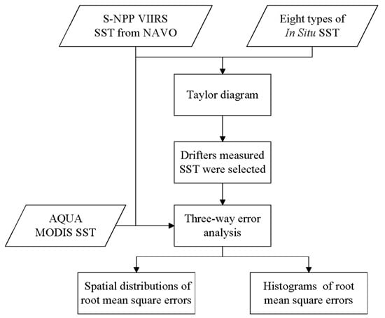
In this paper, we particularly focus on the comparison between global in situ and NAVO S-NPP VIIRS SST. Previous works have shown the difficulty in comparing different sources of SST with their specific characteristics in global and regional scale [2,14,15]. To assess the accuracy of satellite SST, it is important to utilize as many in situ measurements as possible for validation, especially for regions of sparse data. The Taylor diagram is first used to demonstrate the differences of the RMSE, correlation and standard deviation between the NAVO S-NPP VIIRS SST and eight types of in situ measurements, and then select drifter SST as reference to validate the VIIRS SST. Then, a three-way error analysis in conjunction with the drifter and AQUA MODIS SSTs are employed to evaluate the performance of VIIRS SST. The results can be beneficial for other applications, such as the data interpretation, improvement of sensor design, SST retrieval algorithm and merging the VIIRS SST with other available data sources, etc.

This work is organized as follows: the NAVO S-NPP VIIRS, AQUA MODIS and in situ SST used in this work are described in Section 2. A strategy for matching the VIIRS SST and in situ SST and the distribution of the matchups is outlined in Section 3. Then an initial comparison between the VIIRS SST and various types of in situ SST is performed in Section 4. The root mean square error of VIIRS SST is estimated via three-way analyses in Section 5. Conclusions are presented in Section 6.

2. Data

2.1. NAVO S-NPP VIIRS SST

The VIIRS is first on the S-NPP satellite which launched on 28 October 2011 as a part of the Joint Polar Satellite System (JPSS) program [5]. S-NPP is in a sun-synchronous near-polar orbit at 824 km with a swath-width of ~3060 km. As a result, VIIRS provides complete coverage of the globe twice daily without inter-orbit gaps: once in the early afternoon (ascending overpass with a local time node of approximately 13:25) and once in the early morning (descending overpass). The VIIRS provides 22 spectral bands coverage from 0.4–12.5 μm (five imagery bands at ~375 m nadir resolution and 17 moderate resolution bands at ~750 m at nadir). S-NPP VIIRS SST processing relies on five moderate resolution bands (center at 0.67 μm, 0.87 μm, 3.7 μm, 10.7 μm and 12.0 μm) for cloud screening and SST computations. The S-NPP VIIRS is a subsequent sensor of AVHRR and MODIS for SST. The Non-Linear SST (NLSST) algorithm which has been used for MODIS and AVHRR was improved and designated for VIIRS at NAVO [13]. The processing is done in every “target arrays” which is a small granule with 10 × 6 pixel-windows. Cloud-screened and SST retrieved is done on the 2 × 2 pixel unit array, which resulted in the spatial resolution of ~1.5 km.

To avoid the bright reflective of solar radiation, the mid-infrared channel cannot be used in the daytime algorithm as follows:

$$SS{T}_{day}=a_0+a_1{T}_{11}+a_2(T_{11}-T_{12})T_{sfc}+a_3(T_{11}-T_{12})(\sec (\theta )-1)+a_4(T_{11}-T_{12})$$

(1)

where a₀, a₁, a₂, a₃, a₄ are coefficients derived by regression analysis, T₁₁ and T₁₂ are the brightness temperatures at 11 μm (VIIRS band M15) and 12 μm (VIIRS band M16), respectively. T_sfc is a first guess SST that scales the coefficient multiplying the brightness temperature difference between T₁₁ and T₁₂. θ is the sensor zenith angle in radians and this term compensates for the increasing path length when the scan is away from nadir.

The mid-infrared channel is included in the nighttime algorithm as follow:

$$SS{T}_{night}=b_0+b_1{T}_{11}+b_2(T_{3.7}-T_{12})T_{sfc}+b_3(\sec (\theta )-1)+b_4(T_{3.7}-T_{12})$$

(2)

where b₀, b₁, b₂, b₃, b₄ are coefficients derived by regression analysis, T_3.7 is the measured brightness temperature at the mid-infrared channel 3.7 µm (VIIRS band M12). Although the VIIRS measures the skin temperature with infrared sensor, they are regressed to a nominal depth 1 m. There are ~1012 VIIRS granules (~85 s for each granule) every day can be received in near real-time at NAVO. The level 2 NAVO VIIRS SST is integrated to the Group for High-Resolution SST (GHRSST) and quality flags ranging from zero to five are appended to the data follow the GHRSST Data Processing Specification (GHRSST-DPS) [16]. Only the best quality data with flag five are used for validation. They are available at ftp.nodc.noaa.gov/pub/data.nodc/ghrsst/L2P/VIIRS_NPP/NAVO [17].

2.2. MODIS SST

The MODIS is on the AQUA satellite which launched in 2002. The AQUA platform is in a sun-synchronous near-polar orbit at altitude of ~705 km with a local time ascending node of ~13:30. The MODIS measure ±55° from nadir, yielding a swath-width of 2330 km and imaging the entire earth every one to two days at three different spatial resolutions (two bands at 250 m, five bands at 500 m, and 29 bands at 1000 m). It provides 36 channels coverage from 0.4 μm to 14.4 μm. Specifically, the 3.959, 4.05, 11, and 12 µm channels are used for the SST retrieved. The MODIS SST is integrated to the GHRSST through a joint collaboration between the National Aeronautics and Space Administration (NASA) Jet Propulsion Laboratory (JPL), Ocean Biology Processing Group (OBPG), and the RSMAS [18]. The daily MODIS ocean products, such as the Level 1, geolocation, cloud mask products, and higher level geophysical product are processed by OBPG in Hierarchical Data Format (HDF). SST retrieval algorithm, error statistics and quality flagging is in the charge of RSMAS (for more details see [19]). The MODIS 11 µm SST algorithm [20] also uses the nonlinear SST (NLSST) algorithm [21]. Algorithm coefficients are derived via collocations to in situ observations and continuously verified by RSMAS. The coefficients are tuned to three segments depending on the brightness temperature difference (BTD, in °C) between the 11 and 12 µm channels: BTD ≤ 0.5, 0.5 ≤ BTD ≤ 0.9 and BTD ≥ 0.9. During nighttime, the mid-infrared algorithm SST (retrieved from the mid-infrared bands near 4 µm) is used for the baseline SST, while the weekly Reynolds OISST product is bilinear interpolated to the pixel location for the daytime baseline. JPL acquires MODIS level 2 SST from the OBPG in near real-time and reformats them to the GHRSST specification with complete metadata, such as quality flags, in network Common Data Form (netCDF). The MODIS SST is considered to be measurements of the skin layer SST. Approximately 288+ five minute observation granules with ~1 km resolution per day can be achieved from GHRSST via ftp.nodc.noaa.gov/pub/data.nodc/ghrsst/L2P/MODIS_A/JPL [22].

2.3. In Situ Data

In situ subsurface SSTs from five independent data sources obtained from NOAA in situ Quality Monitor (iQuam [23,24]) are used to generate matchups with the satellite data. In addition to four in situ data types (drifters, ships, tropical, and coastal moorings) from the single source, Global Telecommunication System (GTS), four more platform types have been added, including ARGO floats, high-resolution SST drifters (HR-Drifter), coral reef watch (CRW) buoys, and Integrated Marine Observing System (IMOS) track ships. The ships and drifters from GTS are flagged as GTS-Ship and GTS-Drifter to distinguish with the IMOS ships and HR-Drifter, respectively. The tropical moorings (T-mooring) are the moored buoys located at the tropical oceans and the coastal moorings (C-mooring) are the moored buoys located at the coastal areas. The original sampling rate of moored buoys is usually ~10 min and they are usually smoothed at hourly intervals (0000, 0100, 0200…2200, 2300 UTC) to minimize the noise. Drifting buoys observations are also processed into hourly intervals. Some ships take hourly observations, but most take four observations a day at the synoptic reporting hours (0000, 0600, 1200. and 1800 UTC). Argo is an internationally-coordinated program aimed at seeding the global ocean with 3000 profiling floats, which measure temperature and salinity of the upper 2000 m of the ocean [25]. Although Argo floats are designed to shut off at 5 m from the surface in order to avoid contamination/degradation of salinity sensors by pollutants (bio-fouling) at the sea surface and preserve stability, most of them still measure temperature and salinity between 3 and 5 m. They may prove to be a useful global reference for stability as a longer time series accumulates. HR-Drifter is more accurate than the GTS-Drifter. A second decimal place was added in the HR-Drifter temperature in response to high accuracy requests from GHRSST. IMOS ships are from Integrated Marine Observing System (IMOS). CRW is from Coral Reel Watch/NOAA. Since the in situ SSTs sensors are mounted onboard different platforms, maintained by different countries and agencies, the quality of in situ SSTs is often suboptimal and non-uniform. Buoys remain unattended in a hostile environment for years, and ship records are subject to human errors. Additional errors occur during data transmission (to satellite and back to ground), processing and distribution via GTS. The quality assurance for all of the in situ data thus has been done through the NOAA iQuam on a daily basis. A quality flag ranging from zero to five is also appended to the data follows the GHRSST-DPS. Also the best quality data with flag five are used in this study.

3. NAVO S-NPP VIIRS SST—In Situ SST Matchups

3.1. Collocation Criteria

The comparisons are conducted through using extensive collocations between the NAVO S-NPP VIIRS SST and in situ SST during 2014. For each in situ observation, all the near-simultaneous VIIRS observations (within ±1 h) within a radius of 0.05° are selected. Since the in situ observations are organized into daily files, they are collocated with the VIIRS SST from the previous, current, and following day, to ensure accurate collocation at the beginning and end of the daily in situ files. The strict temporal criterion is to limit the influence of possible diurnal warming effects in the surface ocean, which can even reach several degrees at low wind and high insolation conditions [26]. Finally the collocated VIIRS SST is taken an average of the selected values, if and only if, the standard deviation within the collocated window was not exceeding the threshold applied. The standard deviation restriction is an additional filter to reduce the impact from the cloud contamination and suboptimal atmospheric conditions. In this study, the threshold is set as 1 °C.

3.2. Distributions of Matchups

A total number of 90,773 matchups between the VIIRS SSTs and in situ SSTs are obtained during 2014. The number of each type of matchups for daytime and nighttime are summarized in Table 2. The distribution of the matchups is shown in Figure 1. The GTS-Drifter provides a more complete global coverage (Figure 1a). However, their sampling is still sparse and non-uniform in some areas. The fewest of VIIRS-drifting buoy pairs are found in the tropical oceans and the shallow marginal seas. The tropical oceans are characterized by persistent cloud cover and divergent surface currents. The shallow marginal seas with complex topography and human factors lead to few drifting buoys. Figure 1b shows the coverage of other types of matchups. The VIIRS and GTS-Ship matchups are sparse and concentrated around major ship routes in the North Pacific and North Atlantic. There are fewer matchups in the southern hemisphere due to far fewer ships. Additionally, sampling rate of ships is low (as mention in Section 2.3) and the S-NPP VIIRS overpass at fixed local time, which coincide to the ships only in certain limited regions, also lead to fewer matchups. The sampling rate of moored buoys is high, while they are only available in the tropics, along coasts and some other limited areas. Some Argo observations are seen mainly at the deep open oceans. Dense observations of HR-Drifter are seen at north Atlantic and south Indian Ocean. IMOS ships are mainly surrounding the Australian regions and even the Southern Ocean. The VIIRS-CRW pairs are mainly located around the Australian coastal and the coral islands in the open oceans. Although each type of in situ data has some limitations, they seem to be complement to analyze the global errors of the VIIRS SST fully and uniformly.

Table 2. Supplementary statistical information corresponds to Figure 2.

Type	Time	Nums	Bias (°C)	Centered RMS (°C)	σ VIIRS (°C)	σ in Situ (°C)
GTS-Ship	Day	1816	0.05	0.92	8.42	8.55
	Night	3092	0.061	0.78	7.64	7.69
GTS-Drifter	Day	18,093	−0.07	0.39	8.44	8.62
	Night	28,295	−0.06	0.32	7.86	7.87
T-Mooring	Day	755	−0.19	0.54	3.06	3.07
	Night	734	0.09	0.28	3.30	3.28
C-Mooring	Day	4468	0.13	0.54	7.25	7.41
	Night	6488	0.17	0.47	7.38	7.45
Argo	Day	246	0.11	0.54	8.08	8.21
	Night	286	0.01	0.38	7.56	7.56
HR-Drifter	Day	2706	−0.09	0.36	8.04	8.15
	Night	4204	−0.08	0.38	7.73	7.72
IMOS-Ship	Day	8560	0.14	0.58	5.14	5.06
	Night	7583	0.11	0.45	4.02	4.01
CRW	Day	1228	0.07	0.50	1.61	1.59
	Night	2151	0.11	0.42	1.32	1.30

Table 2. Supplementary statistical information corresponds to Figure 2.

Type	Time	Nums	Bias (°C)	Centered RMS (°C)	σ VIIRS (°C)	σ in Situ (°C)
GTS-Ship	Day	1816	0.05	0.92	8.42	8.55
	Night	3092	0.061	0.78	7.64	7.69
GTS-Drifter	Day	18,093	−0.07	0.39	8.44	8.62
	Night	28,295	−0.06	0.32	7.86	7.87
T-Mooring	Day	755	−0.19	0.54	3.06	3.07
	Night	734	0.09	0.28	3.30	3.28
C-Mooring	Day	4468	0.13	0.54	7.25	7.41
	Night	6488	0.17	0.47	7.38	7.45
Argo	Day	246	0.11	0.54	8.08	8.21
	Night	286	0.01	0.38	7.56	7.56
HR-Drifter	Day	2706	−0.09	0.36	8.04	8.15
	Night	4204	−0.08	0.38	7.73	7.72
IMOS-Ship	Day	8560	0.14	0.58	5.14	5.06
	Night	7583	0.11	0.45	4.02	4.01
CRW	Day	1228	0.07	0.50	1.61	1.59
	Night	2151	0.11	0.42	1.32	1.30

Figure 1. Distribution of NAVO S-NPP VIIRS-in situ matchups during 2014: (a) GTS-Drifter (Conventional drifters from GTS) measurements; (b) other types of measurements (GTS-Ship: conventional ships from GTS, T-Mooring: Tropical Moorings, C-Mooring: Coastal Moorings, Argo: Argo floats, HR-Drifter: High resolution drifters, IMOS: IMOS ships, CRW: Coral Reef Watch).

Figure 1. Distribution of NAVO S-NPP VIIRS-in situ matchups during 2014: (a) GTS-Drifter (Conventional drifters from GTS) measurements; (b) other types of measurements (GTS-Ship: conventional ships from GTS, T-Mooring: Tropical Moorings, C-Mooring: Coastal Moorings, Argo: Argo floats, HR-Drifter: High resolution drifters, IMOS: IMOS ships, CRW: Coral Reef Watch).

4. Initial Comparison between the NAVO S-NPP VIIRS SST and in Situ SST

Since various types of in situ SST originate from different countries and agencies for different purpose, it is necessary to identify significant deviations in their suitability for satellite validation first. The Taylor diagram [27] is used to present an overall comparison between different types of fields according to their correlation, centered root-mean squared (RMS) difference, and standard deviations. The correlation coefficient is used to quantify the similarity of different types of data. However, it is impossible to determine the range of variation using only the correlation. The centered RMS is then used to quantify the differences between different types of fields. Moreover, the standard deviations are also needed to give more complete properties for each type of fields. Figure 2 shows an overall comparison between the VIIRS SST and eight types of in situ data in Taylor diagram. The matchups are compartmentalized into daytime and nighttime to examine their difference. The angle to the horizontal axis indicates the correlation. In general, all types of in situ SST have very high correlation (larger than 0.99) with the VIIRS SST except the CRW. The standard deviations of in situ SST are normalized to the VIIRS SST. The VIIRS SST is, thus, located on the horizontal axis with a standard deviation of 1.0. The ratio of standard deviations is the distance from the origin of coordinate. Take the daytime GTS-ship and IMOS ships SST for example, their correlation with the VIIRS SST is similar, but the standard deviation of IMOS is lower than the VIIRS SST, by contrast, the standard deviation of GTS-ship SST is higher than the VIIRS SST. The normalized centered RMS for each type of in situ SST is the distance to the VIIRS SST. The GTS-Drifter and HR-Drifter present the lowest centered RMS errors and highest correlations. It shows a higher clustering around the VIIRS SST during nighttime. It means that the nighttime difference between the in situ SST and the VIIRS SST is a little smaller than the daytime.

Figure 2. Comparisons between the NAVO S-NPP VIIRS SST and different types of in situ SST in Taylor diagram: (a) daytime; and (b) nighttime. Blue dot lines represent the normalized centered RMS error.

Figure 2. Comparisons between the NAVO S-NPP VIIRS SST and different types of in situ SST in Taylor diagram: (a) daytime; and (b) nighttime. Blue dot lines represent the normalized centered RMS error.

The values of centered RMS error and the standard deviation are listed in Table 2. Additionally, the number of matchups and the mean bias (VIIRS-in situ) are also provided to complement the information, since the overall bias has been removed in Taylor diagrams. The overall root-mean-square error (RMSE) can be derived from the square root of the sum of the squares of bias and centered RMS.

The difference is mainly coming from the observation errors by different sensors and the depth at which they measured. Donlon et al. [28] pointed out that the variability of vertical thermal structure at the upper ocean(~10 m) layer is complex, depending on the ocean mixing and air-sea exchange. Since the NAVO S-NPP VIIRS SST are regressed to a nominal depth 1 m, the mooring usually has a thermometer at ~3 m depth, drifter buoys are placed at ~0.2 m depth, ships and Argo measures several meters [29], the difference in near surface temperature vertical gradients should not be neglected. It results in a small positive bias for the NAVO S-NPP VIIRS SST with respect to the in situ SST which at greater depths, except the daytime tropical mooring. It should be caused by the NAVO S-NPP VIIRS SST retrieval algorithm. For the daytime algorithm, only two infrared channels M15 and M16, which are sensitive to columnar water vapor content, are used to derive the SST. In contrast, for the nighttime algorithm, an additional mid-infrared channel M12 is available and especially useful in the high water vapor conditions. The tropical moorings locate in the tropical regions where the water vapor is high. Thus, the high water vapor would affect the radiance in infrared channels and lead to large bias in daytime. A very small negative bias with RMSE less than 0.4 °C for both daytime and nighttime is found between the NAVO S-NPP VIIRS SST and GTS-Drifter and HR-drifter measured SST. Additionally, although a series of strict time and space collocation criteria is adopted in this study, the measurement at different time of day may also contribute to the bias. The centered RMS error of ship SST is higher than other in situ SST when compared with the NAVO S-NPP VIIRS SST.

5. Uncertainties in the VIIRS SST

The aim of validation in this study is to assess the magnitude and characteristics of uncertainties in the NAVO N-SPP VIIRS SST. Considering this, the overall RMSE of in situ measured SST should be small and the distributions of matchups should be uniform in space and time. Therefore, only the GTS-Drifter and HR-drifter (collectively called drifter) matchups are used to validate the NAVO N-SPP VIIRS SST according to the distributions showed in Section 3 and overall error statistics obtained in Section 4. The method of three-way error analysis enables the calculation of standard deviation of error on each observation from the collocations of three different types of observation. The matchups of the NAVO N-SPP VIIRS SST and drifter-measured SST are then collocated to the AQUA MODIS SST under the same match criteria.

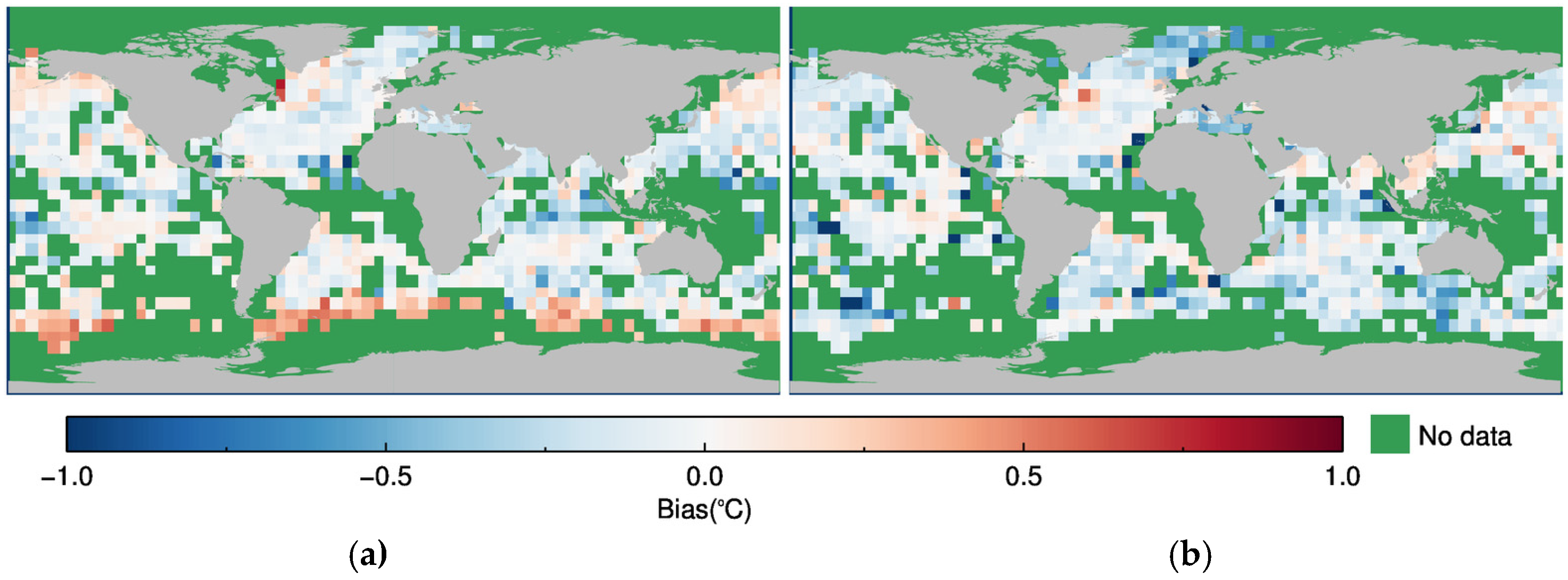
Figure 3 shows the global distribution of mean biases in 5° × 5° boxes for the NAVO N-SPP VIIRS SST and the AQUA MODIS SST with respect to the drifter-measured SST during 2014. The biases are small and uniform in the majority of the global ocean. However, pronounced warm biases in the NAVO N-SPP VIIRS SST even up to 0.5 °C are observed in the Southern Hemisphere at high latitudes. Near-zero biases are observed in MODIS SST in these regions. It means that these biases may be caused by the NAVO N-SPP VIIRS SST retrieval algorithm rather than the nature of the SST.

Figure 3. Global distribution of mean biases in 5° × 5° boxes for (a) the NAVO N-SPP VIIRS SST and (b) the AQUA MODIS SST with respect to the drifter measured SST during 2014.

Figure 3. Global distribution of mean biases in 5° × 5° boxes for (a) the NAVO N-SPP VIIRS SST and (b) the AQUA MODIS SST with respect to the drifter measured SST during 2014.

Three-way error analysis was firstly proposed to validate the wind speeds [30]. O’Carroll et al. [31] made a specific description for this method and applied it to calculate the standard deviation of error on two satellite sensors and drifting buoy SST. Similar analysis has been done to evaluate in situ data for satellite calibration and validation [15]. If the random errors σ are uncorrelated then they can be derived as follows:

$$\begin{array}{l}{\sigma }_D=\sqrt{0.5(V_{DV}+V_{DM}-V_{VM})}\\ {\sigma }_V=\sqrt{0.5(V_{DV}+V_{VM}-V_{DM})}\\ {\sigma }_M=\sqrt{0.5(V_{DM}+V_{VM}-V_{DV})}\end{array}$$

(3)

where D, V, and M indicate the observation types for Drifter, the NAVO N-SPP VIIRS, and the AQUA MODIS, respectively. V_DV is the variance of the difference between Drifter and the VIIRS, V_DM is the variance of the difference between Drifter and MODIS, V_VM is the variance of the difference between the VIIRS and MODIS.

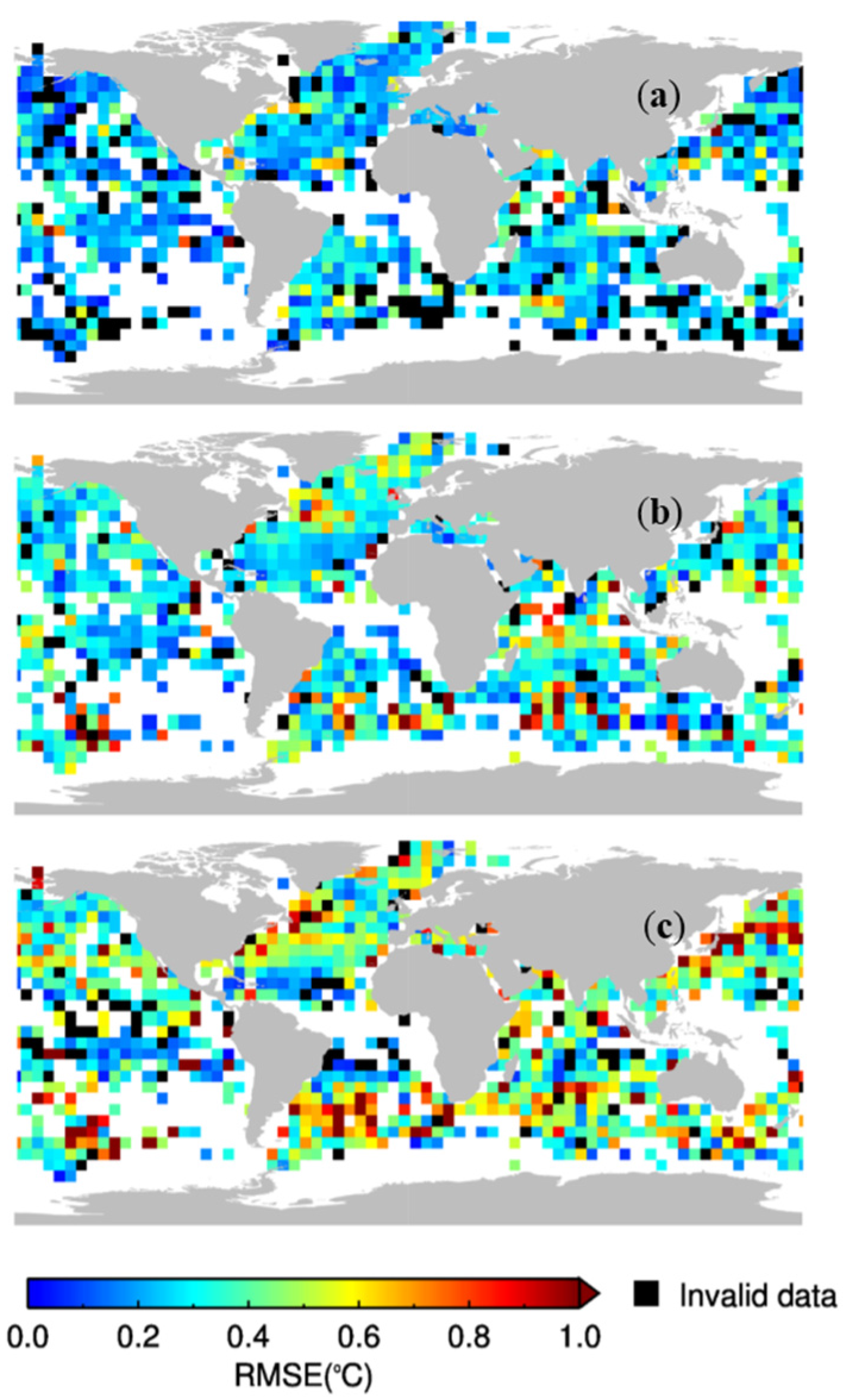
Following O’Carroll et al. [31] and Xu et al. [15], the three-way error analysis is applied in this study to estimate the root mean square error in the NAVO N-SPP VIIRS SST, the drifter-measured SST and the AQUA MODIS SST. The equations have been solved in each 5° × 5° bin, and the results are shown in a form of three maps in Figure 4a,b respectively. In several bins, σ_V, σ_D and σ_M may be not exists when V_DV + V_DM − V_VM < 0, V_DV + V_VM − V_DM < 0 and V_VM + V_DM − V_DV < 0, respectively. It is likely because errors exist in the data or there is a violation of the non-correlation assumption and the respective boxes in Figure 4 are rendered as black color. For the drifter, σ_D values are the smallest and most uniform in the three types of observations. MODIS has the largest and most complex spatial structure of random error. There are large σ_M and σ_V in the Southern Hemisphere at high latitudes, which appear to follow and exist around the Antarctic circumpolar front. Large gradients exist in these regions. The large σ values may be due to real geophysical difference between a point measurement and a spatial average in high spatial varying regions. The diurnal variation usually more prominent in the skin layer which MODIS measures and the mismatch of time may lead to larger difference. Thus, the σ_V values lie between the σ_D and σ_M.

Figure 4. Global maps of root mean square errors (°C) in 5° × 5° resolution for (a) drifter measured SST; (b) NAVO S-NPP VIIRS SST; and (c) AQUA MODIS SST derived from three-way error analysis.

Figure 4. Global maps of root mean square errors (°C) in 5° × 5° resolution for (a) drifter measured SST; (b) NAVO S-NPP VIIRS SST; and (c) AQUA MODIS SST derived from three-way error analysis.

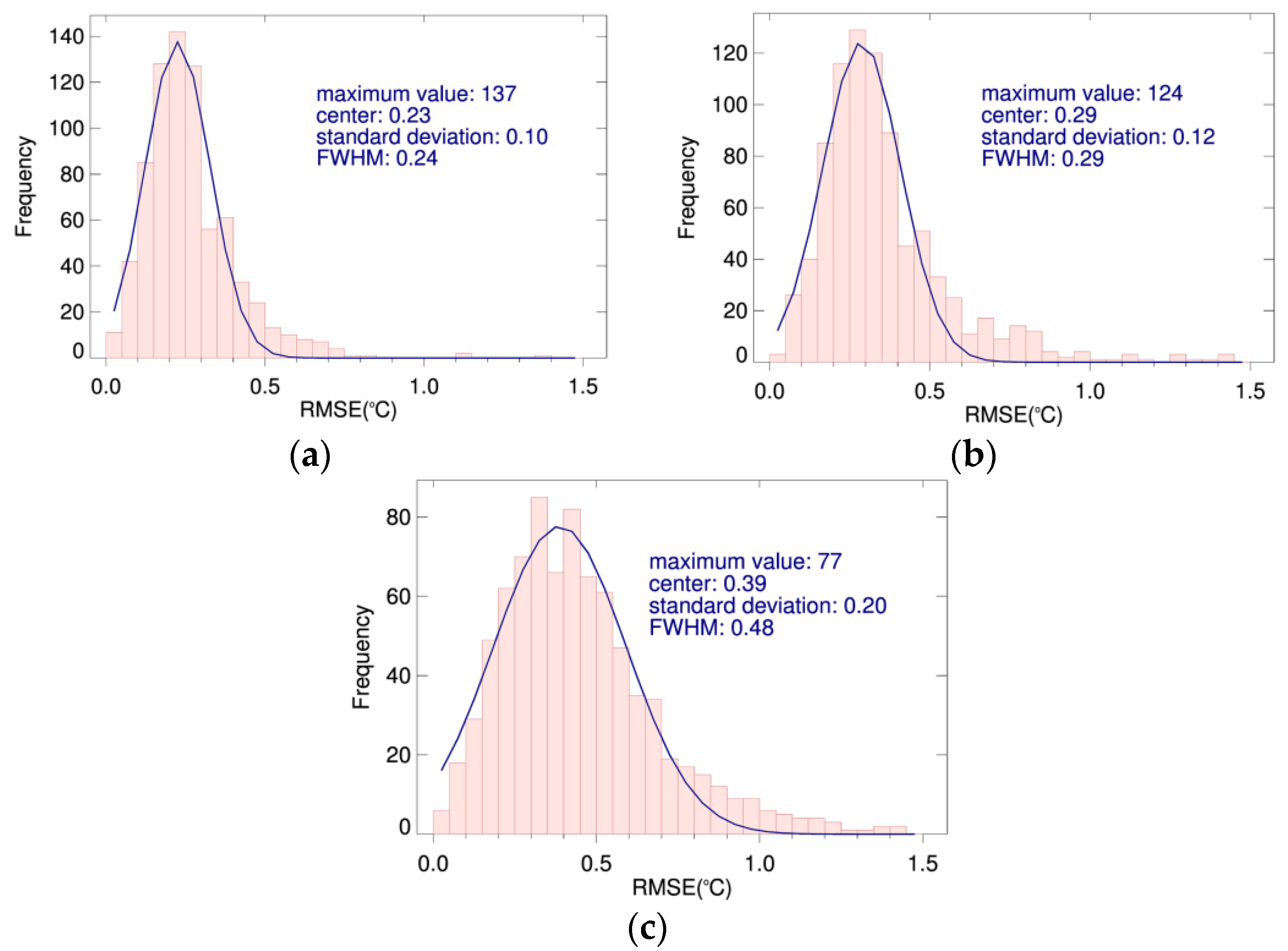
Figure 5 additionally plots histograms of σ_V, σ_D, and σ_M from Figure 4 in 0.05 °C bin width. As expected, the drifting buoy measurements have the smallest error. The value of σ_D varies from 0 to 0.8 °C with a median of ~0.24 °C. This estimate is in good agreement with the estimates of 0.23 °C by O’Carroll et al. [31] and 0.26 °C by Xu et al. [15]. For VIIRS, the RMSE range from 0 to 1 °C with a median of ~0.31 °C. For MODIS, σ_M is ~0.43 °C, but the histogram has a long tail extending out to 1.4 °C. The σ_M lies between previous investigations 0.38 °C [32] and 0.49 °C [33].

Figure 5. Histograms of root mean square errors in 0.05 °C bin width for (a) drifter measured SST; (b) NAVO S-NPP VIIRS SST and (c) AQUA MODIS SST, corresponding to Figure 4. The fitting of the Gaussian function to the RMSE is the blue line, the maximum value, center, standard deviation, and full-width-half-maximum (FWHM) of the Gaussian function are output on the plot as well.

Figure 5. Histograms of root mean square errors in 0.05 °C bin width for (a) drifter measured SST; (b) NAVO S-NPP VIIRS SST and (c) AQUA MODIS SST, corresponding to Figure 4. The fitting of the Gaussian function to the RMSE is the blue line, the maximum value, center, standard deviation, and full-width-half-maximum (FWHM) of the Gaussian function are output on the plot as well.

Ideally, the distribution of random error should be normal. The Gaussian fitting shows normal in the range of 0–0.5 °C, 0–0.6 °C, and 0–0.8 °C for drifter measured SST, NAVO S-NPP VIIRS SST, and AQUA MODIS SST, respectively. However, the long tail on the right side does not fitting well in all the three type of observations. On the one hand, this can mainly result from a variety of causes that relate to how the SST is being made by the individual measurements or retrieval. For infrared remote sensing, the errors may result from the characteristics of the radiometer, and how well the measurements are calibrated, and the atmospheric correction algorithm. On the other hand, the validation techniques are also prone to error. The space-time mismatch leads to errors because of the nature of the SST variable and the temporal-spatial sampling difference in individual observations. Additionally, some of the drifting buoys may be used to derive both the VIIRS SST and MODIS SST retrieval algorithm coefficients, thus they are not completely uncorrelated and the RMSE estimated here may not be fully accurate by using three-way error analysis. The distributed characteristics of the RMSE should be considered for several analysis techniques, as in data assimilation and the merging of the satellite and in situ datasets.

6. Conclusions

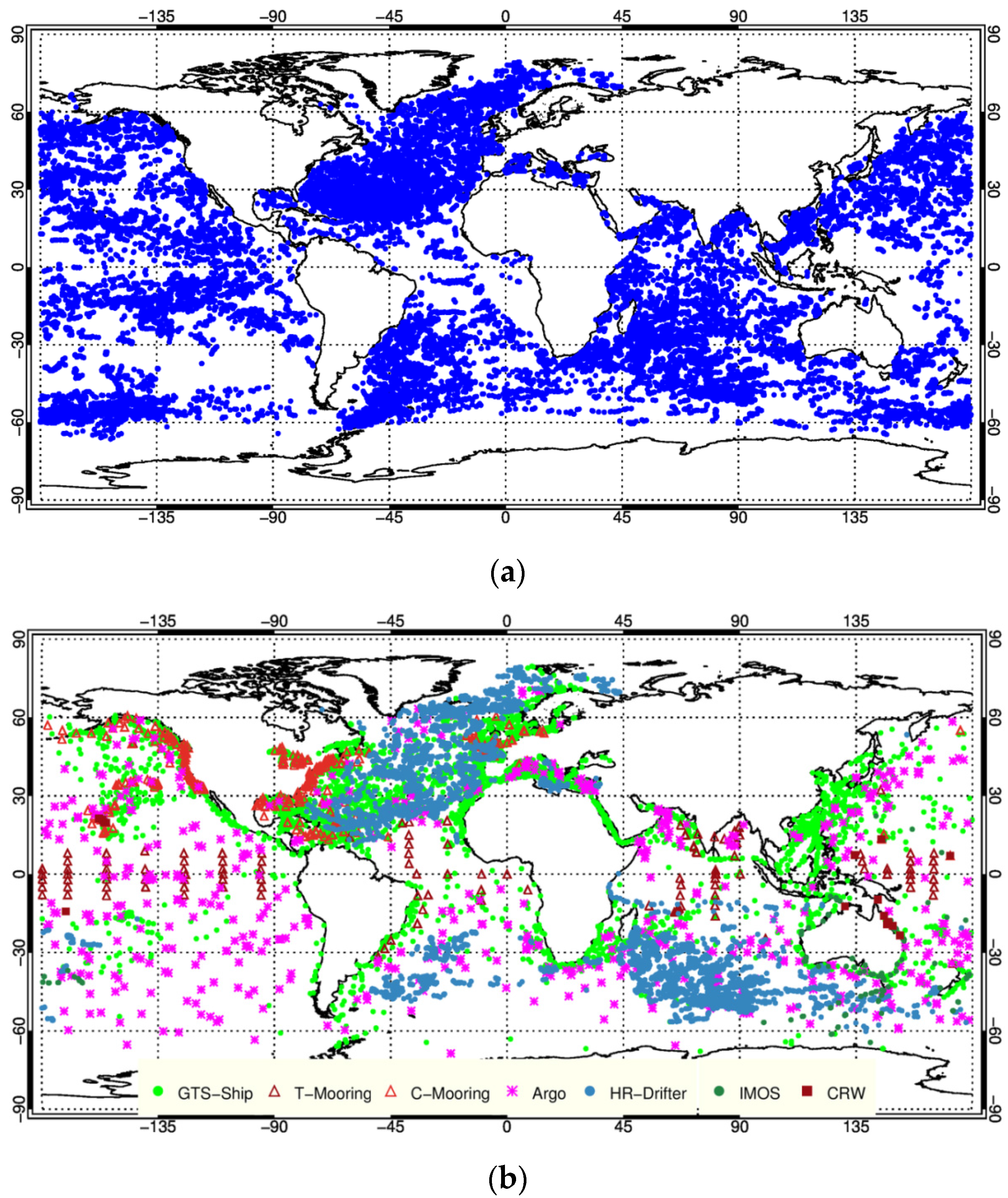
This study was devoted to the analysis of the magnitude and characteristics of uncertainties in the NAVO S-NPP VIIRS SST. Eight types of in situ SST from five independent sources were collocated to the VIIRS SST within ±1 h and within ±0.05° of latitude and longitude. The distribution of the matchups shows that the drifters provide densest and most complete global coverage and other types of in situ data are only available in some limited areas.

An overall comparison results are performed in Taylor diagrams. They show that all types of in situ SST have very high correlation with the VIIRS SST except the CRW. The GTS-Drifter and HR-Drifter present very small negative mean bias and lowest center RMS errors less than 0.4 °C for both daytime and nighttime. For other types of in situ observations, ships measured SST have the largest center RMS errors 0.78 °C and 0.92 °C for nighttime and daytime, respectively, and positive mean bias exist. The bias may be due to the vertical gradients in near surface temperature. The NAVO VIIRS SST is at a nominal 1 m depth, which is deeper than the drifter measured SST and shallower than other in situ SST. However, a highest negative bias exists in the daytime tropical mooring. It may be due to the water vapor influence of daytime NAVO S-NPP VIIRS SST retrieval algorithm or time mismatch within 1 h when diurnal warming happening, or both.

Based on the overall comparison, drifters measured SSTs are selected to further investigate the uncertainty in the NAVO S-NPP VIIRS SST. Another SSTs retrieved from AQUA MODIS are used to help the analysis. The three-way error analysis shows that the errors are smallest and most uniform in drifter while largest and with most complex spatial structure in AQUA MODIS SST. The NAVO S-NPP VIIRS SST lie between the drifters measured SST and AQUA MODIS SST with high accuracy, and at a median RMSE of~0.31 °C ranging from 0–1 °C. The distribution of errors shows normality except for the long tail part on the right side and this should be considered when the SST are merged with other observations or assimilated into models. Global distribution of NAVO S-NPP VIIRS SST minus drifters measured SSTs shows pronounced warm biases up to 0.5 °C in the Southern Hemisphere at high latitudes, while near-zero biases are observed in AQUA MODIS SST minus drifters measured SSTs. It means that these biases may be caused by NAVO S-NPP VIIRS SST retrieval algorithm rather than the nature of the SST. The reasons and correction for this bias need to be further studied.

References

1. Donlon, C.J.; Casey, K.S.; Robinson, I.S.; Gentemann, C.L.; Reynolds, R.W.; Barton, I.; Arino, O.; Stark, J.; Rayner, N.; Leborgne, P.; et al. The godae high-resolution sea surface temperature pilot project. Oceanography 2009, 22, 34–45. [Google Scholar] [CrossRef]
2. Castro, S.L.; Wick, G.A.; Jackson, D.L.; Emery, W.J. Error characterization of infrared and microwave satellite sea surface temperature products for merging and analysis. J. Geophys. Res.-Oceans 2008, 113. [Google Scholar] [CrossRef]
3. Reynolds, R.W.; Smith, T.M.; Liu, C.; Chelton, D.B.; Casey, K.S.; Schlax, M.G. Daily high-resolution-blended analyses for sea surface temperature. J. Clim. 2007, 20, 5473–5496. [Google Scholar] [CrossRef]
4. Donlon, C.J.; Martin, M.; Stark, J.; Roberts-Jones, J.; Fiedler, E.; Wimmer, W. The operational sea surface temperature and sea ice analysis (ostia) system. Remote Sens. Environ. 2012, 116, 140–158. [Google Scholar] [CrossRef]
5. Cao, C.; Xiong, J.; Blonski, S.; Liu, Q.; Uprety, S.; Shao, X.; Bai, Y.; Weng, F. Suomi npp viirs sensor data record verification, validation, and long-term performance monitoring. J. Geophys. Res.-Atmos. 2013, 118. [Google Scholar] [CrossRef]
6. Cao, C.; de Luccia, F.J.; Xiong, X.; Wolfe, R.; Weng, F. Early on-orbit performance of the visible infrared imaging radiometer suite onboard the suomi national polar-orbiting partnership (s-npp) satellite. IEEE Trans. Geosci. Remote Sens. 2014, 52, 1142–1156. [Google Scholar] [CrossRef]
7. Uprety, S.; Cao, C.Y. Suomi npp viirs reflective solar band on-orbit radiometric stability and accuracy assessment using desert and antarctica dome c sites. Remote Sens. Environ. 2015, 166, 106–115. [Google Scholar] [CrossRef]
8. Lei, N.; Wang, Z.P.; Xiong, X.X. On-orbit radiometric calibration of suomi npp viirs reflective solar bands through observations of a sunlit solar diffuser panel. IEEE Trans. Geosci. Remote Sens. 2015, 53, 5983–5990. [Google Scholar] [CrossRef]
9. Liang, X.; Ignatov, A. Avhrr, MODIS, and VIIRS radiometric stability and consistency in sst bands. J. Geophys. Res.-Oceans 2013, 118, 3161–3171. [Google Scholar] [CrossRef]
10. Liu, Y.; Yu, Y.; Yu, P.; Göttsche, F.M.; Trigo, I.F. Quality assessment of s-npp viirs land surface temperature product. Remote Sens. 2015, 7, 12215–12241. [Google Scholar] [CrossRef]
11. Petrenko, B.; Ignatov, A.; Kihai, Y.; Stroup, J.; Dash, P. Evaluation and selection of sst regression algorithms for jpss viirs. J. Geophys. Res.: Atmos. 2014, 119, 4580–4599. [Google Scholar] [CrossRef]
12. McKenzie, B.; May, D.; Cayula, J.-F.; Willis, K. Initial results of npp viirs sst processing at navoceano. Ocean Sens. Monit. IV 2012, 8372. [Google Scholar] [CrossRef]
13. Cayula, J.-F.P.; May, D.A.; McKenzie, B.D.; Willis, K.D. Viirs-derived sst at the naval oceanographic office: From evaluation to operation. Ocean Sens. Monitor. V 2013, 8724. [Google Scholar] [CrossRef]
14. Emery, W.J.; Baldwin, D.J.; Schlussel, P.; Reynolds, R.W. Accuracy of in situ sea surface temperatures used to calibrate infrared satellite measurements. J. Geophys. Res.-Oceans 2001, 106, 2387–2405. [Google Scholar] [CrossRef]
15. Xu, F.; Ignatov, A. Evaluation of in situ sea surface temperatures for use in the calibration and validation of satellite retrievals. J. Geophys. Res. Oceans 2010, 115. [Google Scholar] [CrossRef]
16. Donlon, C.; Robinson, I.; Casey, K.S.; Vazquez-Cuervo, J.; Armstrong, E.; Arino, O.; Gentemann, C.; May, D.; LeBorgne, P.; Piolle, J.; et al. The global ocean data assimilation experiment high-resolution sea surface temperature pilot project. Bull. Am. Meteorol. Soc. 2007, 88, 1197–1213. [Google Scholar] [CrossRef]
17. S-NPP VIIRS L2P Sea Surface Temperature from NAVO. Available online: ftp.nodc.noaa.gov/pub.data.nodc/ghrsst/L2P/VIIRS_NPP/NAVO (accessed on 23 August 2015).
18. Brown, O.B.; Minnett, P.J.; Evans, R.; Kearns, E.; Kilpatrick, K.; Kumar, A.; Sikorski, R.; Závody, A. Modis Infrared Sea Surface Temperature Algorithm Algorithm Theoretical Basis Document Version 2.0; University of Miami: Coral Gables, FL, USA, 1999. [Google Scholar]
19. OceanColor documents. Available online: http://oceancolor.gsfc.nasa.gov/DOCS/modis_sst/ (accessed on 20 November 2012).
20. Franz, B. Implementation of sst processing within the obpg. Último Acceso 2006, 4, 2014. [Google Scholar]
21. Walton, C.C. Nonlinear multichannel algorithms for estimating sea surface temperature with AVHRR satellite data. J. Appl. Meteorol. 1988, 27, 115–124. [Google Scholar] [CrossRef]
22. AQUA MODIS L2P Sea Surface Temperature from JPL. Available online: ftp.nodc.noaa.gov/pub/data.nodc/ghrsst/L2P/MODIS_A/JPL (accessed on 23 August 2015).
23. Xu, F.; Ignatov, A. In situ SST quality monitor (i quam). J. Atmos. Ocean. Technol. 2014, 31, 164–180. [Google Scholar] [CrossRef]
24. Ignatov, A.; Xu, F. In situ SST quality monitor: From iquam version 1 to version 2. In Proceedings of the 14th GHRSST Meeting, Woods Hole, MA, USA, 17 June 2013.
25. Roemmich, D.; Johnson, G.C.; Riser, S.; Davis, R.; Gilson, J.; Owens, W.B.; Garzoli, S.L.; Schmid, C.; Ignaszewski, M. The argo program observing the global ocean with profiling floats. Oceanography 2009, 22, 34–43. [Google Scholar] [CrossRef]
26. Kawai, Y.; Wada, A. Diurnal sea surface temperature variation and its impact on the atmosphere and ocean: A review. J. Oceanogr. 2007, 63, 721–744. [Google Scholar] [CrossRef]
27. Taylor, K.E. Summarizing multiple aspects of model performance in a single diagram. J. Geophys. Res.-Atmos. 2001, 106, 7183–7192. [Google Scholar] [CrossRef]
28. Donlon, C.J.; Minnett, P.J.; Gentemann, C.; Nightingale, T.J.; Barton, I.J.; Ward, B.; Murray, M.J. Toward improved validation of satellite sea surface skin temperature measurements for climate research. J. Clim. 2002, 15, 353–369. [Google Scholar] [CrossRef]
29. Sybrandy, A.; Niiler, P.; Martin, C.; Scuba, W.; Charpentier, E.; Meldrum, D. Global Drifter Programme Drifter Design Reference; DBCP Report; Data Buoy Cooperation Panel: Paris, France, 2009. [Google Scholar]
30. Stoffelen, A. Toward the true near-surface wind speed: Error modeling and calibration using triple collocation. J. Geophys. Res.-Oceans 1998, 103, 7755–7766. [Google Scholar] [CrossRef]
31. O’Carroll, A.G.; Eyre, J.R.; Saunders, R.W. Three-way error analysis between aatsr, amsr-e, and in situ sea surface temperature observations. J. Atmos. Ocean. Technol. 2008, 25, 1197–1207. [Google Scholar] [CrossRef]
32. Gentemann, C.L. Three way validation of MODIS and AMSR-E sea surface temperatures. J. Geophys. Res.: Oceans 2014, 119, 2583–2598. [Google Scholar] [CrossRef]
33. Minnett, P.J. The validation of sea surface temperature retrievals from spaceborne infrared radiometers. In Oceanography from Space; Springer: Berlin, Germany, 2010; pp. 229–247. [Google Scholar]