Article

Radarsat-2 Backscattering for the Modeling of Biophysical Parameters of Regenerating Mangrove Forests

by
Michele F. Cougo
1,
Pedro W. M. Souza-Filho
1,2,*,
Arnaldo Q. Silva
1,
Marcus E. B. Fernandes
3,
João R. dos Santos
4,
Maria R. S. Abreu
1,
Wilson R. Nascimento
1 and
Marc Simard
5
1
Geoscience Institute, Universidade Federal do Pará, Cidade Universitária, P.O. Box 8608, 66075-110 Belém, Pará, Brazil
2
Vale Institute of Technology, Rua Boaventura da Silva, 955, 66055-090 Belém, Pará, Brazil
3
Laboratory of Mangrove Ecology, Institute of Coastal Studies, Universidade Federal do Pará, Campus de Bragança, 68600-000 Bragança, Pará, Brazil
4
National Institute for Space Research—INPE, Remote Sensing Department, 12227-010 São José dos Campos, São Paulo, Brazil
5
California Institute of Technology, Jet Propulsion Laboratory, MS 300-319D, 4800 Oak Grove Dr., Pasadena, CA 90039, USA
*
Author to whom correspondence should be addressed.
Remote Sens. 2015, 7(12), 17097-17112; https://doi.org/10.3390/rs71215873
Submission received: 31 August 2015 / Revised: 27 November 2015 / Accepted: 9 December 2015 / Published: 17 December 2015
(This article belongs to the Special Issue Remote Sensing of Mangroves: Observation and Monitoring)

Abstract

:
The aim of this study is to understand the relationship between radar backscattering (σ°, β° and γ) of a multi-polarized Radarsat-2 C-band image with the structural attributes of regenerating mangrove vegetation located at the mouth of the Amazon River. CBH (circumference at breast height), height and species data were collected to characterize vegetation structure and above-ground biomass (AGB) at 17 plots with a total of 3090 measured individuals. Significant relationships between the linear σ° in VH (vertical transmit, horizontal receive) cross-polarization produced r2 values of 0.63 for the average height, 0.53 for the DBH, 0.46 for the basal area (BA) and 0.52 for the AGB. Using co-polarized HH (horizontal transmit, horizontal receive) and VV (vertical transmit, vertical receive), r2 values increased to 0.81, 0.79, 0.67 and 0.79, respectively. Vegetation attribute maps of average canopy height, DBH and AGB were generated for the study area. We conclude that multi-polarized Radarsat-2 images were adequate for characterization of vegetation attributes in areas of mangrove regeneration.

Graphical Abstract

1. Introduction

Mangroves are among the most productive ecosystems in the world [1], exporting nutrients and organic matter to adjacent waters and coastal environments, and providing for a complex aquatic food web [1,2]. Mangroves have great economic and ecological significance, protecting and stabilizing the coastline, and acting as nurseries and breeding grounds for numerous wildlife species, valuable goods and services [3,4,5,6].
Mangrove productivity is directly linked to biomass, which is important for understanding the cycling of organic matter in mangrove ecosystems [6]. A traditional method of estimating biomass is by manually measuring structural parameters of vegetation through allometric equations. Measuring these parameters by non-destructive means is a challenge that has been reported by many authors in Africa [7], Europe [8], the Americas, Asia, and Oceania [9,10,11,12,13].
Research studies have attempted to produce inventories and establish efficient approaches for the monitoring and conservation of mangroves [1,3,5,14,15]. However, these ecosystems are difficult to access because of the maze of roots and stems, and unconsolidated substrate and flood tides [16]. Thus, remote sensing imaging with different spectral frequencies and spatial and temporal resolutions has proven to be a more efficient source of data to study the dynamics of mangrove forests at large scales [17,18,19,20,21,22]. This paper investigates the use of synthetic aperture radar (SAR) in regenerating mangrove forests. Radar instruments operate in the microwave spectrum and make a suitable sensor to monitor low-latitude environments characterized by the frequent presence of clouds, rain and smoke.
Radar backscatter results from microwaves reflected from vegetation components, such as twigs, branches and trunks [23,24]. Several studies have related radar backscattering with the structural parameters of mangrove vegetation such as homogeneous forest canopies to estimate above-ground biomass (AGB) [25,26,27,28,29]. Recently, Kovacs et al. [30,31] estimated structural attributes of degraded mangrove forests on the Pacific coast of México using multi-polarized C-band (Radarsat-2) and L-band images (ALOS PALSAR). The mangrove area is the focus of this study and it is located in the Bragança Peninsula (northeastern coast of Pará) along the northern coast of Brazil. The region has undergone significant anthropic pressure in the last 30 years because of the construction of a highway to facilitate access to coastal resources by the local population and allow mangrove products to be transported to local markets [32]. The highway slices the intertidal mud flat deposits that are densely colonized by mangrove forests over a stretch of 25 km, thus modifying the hydrological regime and causing significant die-off of vegetation that was subsequently removed by the local population. After a few years, part of this degraded area showed incipient natural regeneration [21].
This study aims to evaluate the relationship between the structural attributes of the regenerating mangrove vegetation and multi-polarized data from the Radarsat-2 (C-band) sensor using statistical regression models. The correlation between radar attributes (i.e., σ°, β° and γ) at the four polarization configurations (horizontal transmit, horizontal receive—HH, horizontal transmit, vertical receive—HV, vertical transmit, horizontal receive—VH and vertical transmit and vertical receive—VV) and the mangrove structure data (diameter at breast height—DBH, basal area—BA, height and biomass) was investigated. Finally, the regression models are used to generate forest structure maps of a regenerating mangrove in order to support implementation of rehabilitation and restoration efforts.

2. Data and Methods

2.1. Study Area

The study area is located along the northern coast of Brazil approximately 380 km southeast of the mouth of the Amazon River (Figure 1). It is part of the largest continuous mangrove belt in the world [22,33]. The climate is classified as hot and humid [34] with two seasons, rainy (January to July) and dry (August to January), which have an average rainfall of 2000 mm and 20 mm, respectively [35]. The region boasts a semidiurnal macrotidal regime with minimum variations of 1.8 m and maximum variations of 5.4 m [36]. The mangroves of the Bragança Peninsula occupy an area of 466 km2 over extensive mud flats up to 30 km wide and are located between the high levels of spring and mean tide level [37].
The floristic composition of the mangrove vegetation in the region is composed of four mangrove species: Rhizophora mangle L. (Rhizophoraceae), Avicennia germinans (L.) L., Avicennia schaueriana Stapf and Leechman (Acanthaceae) and Laguncularia racemosa (L.) CF. Gaertn. (Combretaceae). The species R. mangle is predominant [38]. Despite the low variety in species, there is a great variability in the structure of the mangrove forest because of topography and local hydrological conditions [39].
Figure 1. Map of the study area: (A) SRTM and (B) RapidEye image in 1R2G3B normal color composition. The figure also shows the location of the 17 plots analyzed in this study.
Remotesensing 07 15873 g001

2.2. SAR Data and Image Processing

The SAR data used in this investigation were a multi-polarized Radarsat-2 image (Table 1) obtained in fine-beam mode (FQ5). Precipitation and tide data were provided by the National Institute of Meteorology [40] and Directorate of Hydrography and Navigation of the Brazilian Navy [41], respectively. An optical image obtained with the REIS (RapidEye Earth Imaging System) sensor acquired on 18 July 2011 was used to facilitate the location of field plots.
Table 1. Characteristics of the SAR image and environmental conditions on the acquisition day.
Sensor RADARSAT-2
Frequency GHz (band)5.40 (C)
Wavelength5.6 cm
PolarizationHH/HV/VH/VV
Acquisition modeFine Quad-Pol
Level processingSingle Look Complex–SLC
Data type (n looks)Polarimetric (1)
Nominal resolution11 × 9 m
Pixel spacing4.73 (range) and 4.98 (azimuth)
Orbit of acquisitionDescending
Acquisition date6 November 2010
Time of acquisition08:55:58
Incidence angle23.39°–25.28°
Precipitationno rain
Tide Condition+3 m
The Shuttle Radar Topography Mission (SRTM) digital elevation model with 11 ground control points (GCP) was used for image orthorectification. This step was developed with the use of Toutin’s Radargrammetic model [42] implemented in the application OrthoEngine/PCI; the Root Mean Square Error (RMSE) was 12.2 m, 12.19 m and 12.58 m for the σ°, β° and γ images, respectively. Subsequently, the speckle noise was reduced with the use of the enhanced Lee filter [43]. Among the three applied window sizes (3 × 3, 5 × 5 and 7 × 7 pixels), the 5 × 5 pixel size was shown in a previous study to provide a better performance in the analysis of the correlations with the biophysical parameters. These processing steps were performed for the three reflectivity parameters (σ°, β° and γ), representing the reflected microwave as: sigma (σ°) the average reflectivity of a sample of target normalized by the unit area in the ground range; gamma (γ) the reflectivity measured in terms of forward incident wave; and beta (β°) the reflectivity in slant range which is independent of the local incident angle [16]. The use of parameter σ° in studies based on backscattering is a consensus in the literature [16,26]. However, we also investigated the relationship of γ and β° parameters with vegetation parameters based on the fact that γ will remain approximately constant for all incidence angles, and thus is a more convenient measurement parameter to employ than σ° when dealing with volume scattering targets, such as forest. The β° parameter is independent of the local topography and it represents the only directly measure from image radar system, what is known as “radar brightness” [44]. Subsequently, the average backscattering values of the three radar attributes were extracted for each investigated plot of 100 m2.

2.3. Collecting Structural Data in the Mangrove Forest

Initially, before fieldwork, six classes were visually distinguished in the RapidEye image to determine the local vegetation gradient: exposed ground, recent stage, initial regeneration, intermediate regeneration, advanced regeneration, and flooded vegetation. To extract backscattering values from the Radarsat-2 image, 20 plots were defined over the SAR image to characterize the six initial classes, totaling 120 plots. To reduce the number of plots to be inventoried during the fieldwork, a plot cluster analysis was performed based on the backscattering values. Hence, 17 plots were selected to be inventoried during the fieldwork carried out in August and December 2012. The central and corner coordinates of each plot were determined with the use of a differential global positioning system (DGPS—model ASTECH Z-Xtreme) with decimeter accuracy. The determination of the corner coordinates of each plot was carried out with a TOPCON total station model GTS 210. The position of each tree and shrub present in the plot were obtained in the same manner. The size of the plots (10 × 10 m) was defined according to the nominal resolution (11 × 9 m) of the Radarsat-2 Fine Quad Pol 5 mode, equivalent to approximately four pixels of this SAR image; this plot size is adequate due to high mangrove vegetation density [45].
The botanical species were identified and biophysical parameters, such as the circumference at breast height (CBH) and height of the individuals, were measured in each plot with their respective geographical positions. For low stature trees without trunks at 1.30 m (CBH), the circumference measurement was performed below the first branch, which was proposed by Soares [46]. Subsequently, the diameters at breast height (DBH), basal area (BA), mean and maximum heights and density values were calculated according to Cíntron and Schaeffer Novelli [45]. Lorey’s height was also calculated for each plot [47]. After the collection of biophysical parameters, exposed ground class without vegetation was not included in the statistical analysis and flooded vegetation was recognized as the advanced regeneration class. Hence, four classes were redefined as recent stage, initial regeneration, intermediate regeneration and advanced regeneration. The recent stage is characterized as being bare soil with recent colonization of single seedlings of mangrove vegetation (average BA of 2.9 m2·ha−1). The initial stage of regeneration has less exposed soil due to occurrence of small shrubs (average BA of 9 m2·ha−1). In the intermediate regeneration stage the soil is covered by vegetation with more structural development (average BA of 14 m2·ha−1), but lower than that of the advanced regeneration stage, where the trees can reach 15 m in height and an average BA of 20 m2·ha−1 (Figure 2).
After the biophysical data were processed, a cluster analysis was performed to associate plots with similar structural development of the canopy. The average canopy height, DBH and BA were analyzed through the Euclidean distance method. An analysis of variance (ANOVA) was applied to the formed clusters to investigate significant differences in the distribution of the structural parameters. Subsequently, the post-hoc Tukey’s test [48] characterized the differences within the clusters by multiple comparisons of the paired clusters.
Figure 2. (A) Cluster analysis using Euclidian distance with the biophysical parameters: average canopy height, DBH and basal area; (B) Different mangrove regeneration stages observed in the field.
Remotesensing 07 15873 g002

2.4. Estimation of the Above-Ground Biomass

The allometric equations proposed by Fromard et al. [49] for the mangroves of French Guiana were used to estimate the AGB of the study area. There are no specific allometric equations for mangrove trees along the coast of the Brazilian Amazon. When developing Equations (1) to (4), Fromard et al. [49] indicated that the independent variable DBH was used because it is a parameter that can be measured for all individuals more accurately than height.
Avicennia germinans: 1 cm < DBH < 4 cm: y = 200.4 DBH2,1 (g)
DBH > 4 cm: y = 0.14 DBH2,4 (Kg)
Laguncularia racemosa: y = 102.3 DBH2,5 (g)
Rhizophora spp.: y = 128.2 DBH2,6 (g)
Based on the above equations, our dataset spans a range of AGB of 0.5–2.8 kg (DBH < 4 cm) and 5.7–1543.7 kg (DBH > 4 cm) for A. germinans, 0.3–27.6 kg for L. racemosa and 0.3–1036.6 kg for Rhizophora spp. Plots were then rearranged in order of increasing AGB to facilitate the presentation of data and discussion.

2.5. Modeling the Impact of Forest Structure in Regenerating Mangrove on SAR Data

Analysis of the relationship between the structural attributes and the multi-polarized backscattering of the Radarsat-2 image was performed using simple and multiple regression statistical methods in which the independent variables were the backscattering values and structural attribute values were the dependent variables. The development of the models followed the methodology described by Neter et al. [50] with various functions: linear, logarithmic, second- and third-order polynomial, power and exponential.
In the multiple linear regression model, the selection of the variables was based on the best subset [50] regressive method and decision criteria (r2, r2 fit and Cp Mallow) in which the best fit with the fewest possible explanatory variables is identified. The validation of the developed models was performed by the methods PRESS (Prediction Sum of Squares) and RMSE (Root Mean Square Error).

3. Results and Discussion

3.1. SAR Attributes of the Mangrove Features

The mean backscattering values on a linear scale extracted from the Radarsat-2 image for each of the studied plots are shown in Table 2. The cross-polarization channels showed backscattering values lower than the co-polarization channels for all reflectivity parameters. While the expected strong surface and double-bounce scattering is observed in co-polarized images, lower backscatter is observed at cross-polarizations, which results mainly from the volume scattering occurring within the mangrove canopies [26].
Table 2. Mean backscattering values in σ°, β° and γ extracted for each plot (P). See Figure 3 for the location of the plots.
Pσ°HHσ°HVσ°VHσ°VVβ°HHβ°HVβ°VHβ°VVγHHγHVγVHγVV
Recent stage10.1170.0090.0110.2420.1450.0250.0220.5560.1810.0110.0150.26
20.1310.0020.0010.0650.280.0120.010.2150.160.0170.0070.165
30.1480.0290.030.0770.4150.1230.0980.2990.1640.0410.0410.149
40.0180.0060.0060.1090.0710.0190.0150.2090.0690.0090.0060.173
50.0450.0280.0390.3010.2980.0570.0850.2840.1890.0270.0480.133
60.3190.0330.030.6961.2420.1010.1042.3550.0820.0370.0290.522
Initial r.70.1040.0270.0230.0880.5350.0920.050.4110.1750.0150.0150.087
80.2410.0020.0050.0630.4470.020.0060.2140.3520.0320.0240.502
90.4960.0330.0280.4363.2950.0840.0780.8560.5650.050.0520.384
100.2220.0240.0280.2050.8330.0540.0640.6951.1990.0280.030.193
110.0730.0070.0080.0421.0960.0130.0240.5030.1650.0190.0220.072
Int. r.120.2590.0090.0150.1980.5890.0930.0770.170.0640.0460.0460.073
130.0920.0850.0780.110.2950.2110.1910.1740.1670.0840.0770.224
Advanced r.140.1450.0770.0730.1170.1040.1410.140.0940.1980.0760.0770.232
150.30.0290.0320.1260.9990.0690.0830.2560.1330.0560.0590.306
160.3460.0710.0490.0690.9350.1790.0980.3560.3450.0430.0330.114
170.4930.0390.090.2761.1320.1640.2220.6450.3640.0280.060.274
P = plot; Initial r. = initial regeneration; Int. r. = intermediate regeneration; Advanced r. = advanced regeneration.
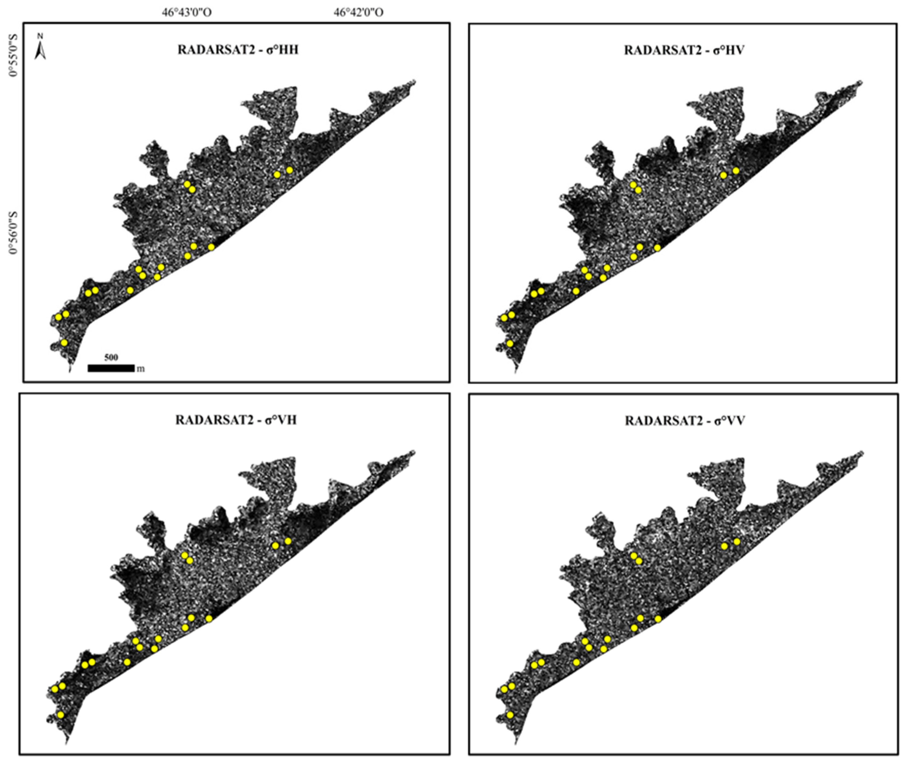
The Radarsat-2 image in its different polarizations and locations of the 17 plots studied in the field is shown in Figure 3. The observed spatial patterns in the Radarsat-2 HV image generally follow the pattern described by Souza-Filho and Paradella [21] with strong and low backscatter in regeneration and cleared areas, respectively. The co-polarized (i.e., HH and VV) images showed less distinction between those vegetation types. Kovacs et al. [17] reported that co-polarized scattering could not be used to distinguish healthy from dead mangroves. It was also observed that the high backscatter from healthy stands is related to very high crown volume scattering from the canopy (branches and leaves), while backscatter from dead and regenerating mangroves is dominated by a double-bounce scattering mechanism from standing water below the canopy acting with the trees as corner reflectors.
The predominance of higher signal returns in the central portion of all of the images (Figure 3) suggests a greater presence of vegetation, which contributes to the occurrence of double-bounce scattering, as a result of trunk-ground interactions during high tides that reach 6 m in range. In addition, C-band images present a higher sensitivity to canopy components which substantially increases scattering at the canopy surface in addition to volume scattering.
Figure 3. Radarsat-2 image in the four polarizations with the locations of the plots studied in the field.
Remotesensing 07 15873 g003

3.2. Analysis of Canopy Structure in Regenerating Mangroves

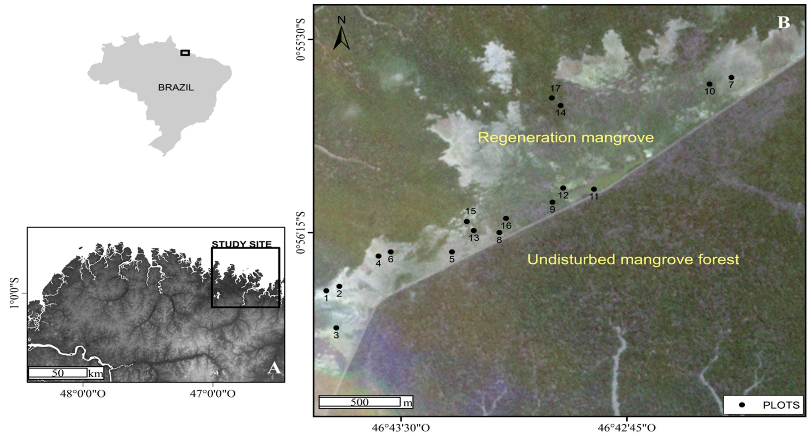
The total area of the studied plots was 1700 m2 in which 2510 live individuals of A. germinans, 261 individuals of L. racemosa, and 30 individuals of R. mangle were measured in addition to 289 dead individuals for a total of 3090 individuals.
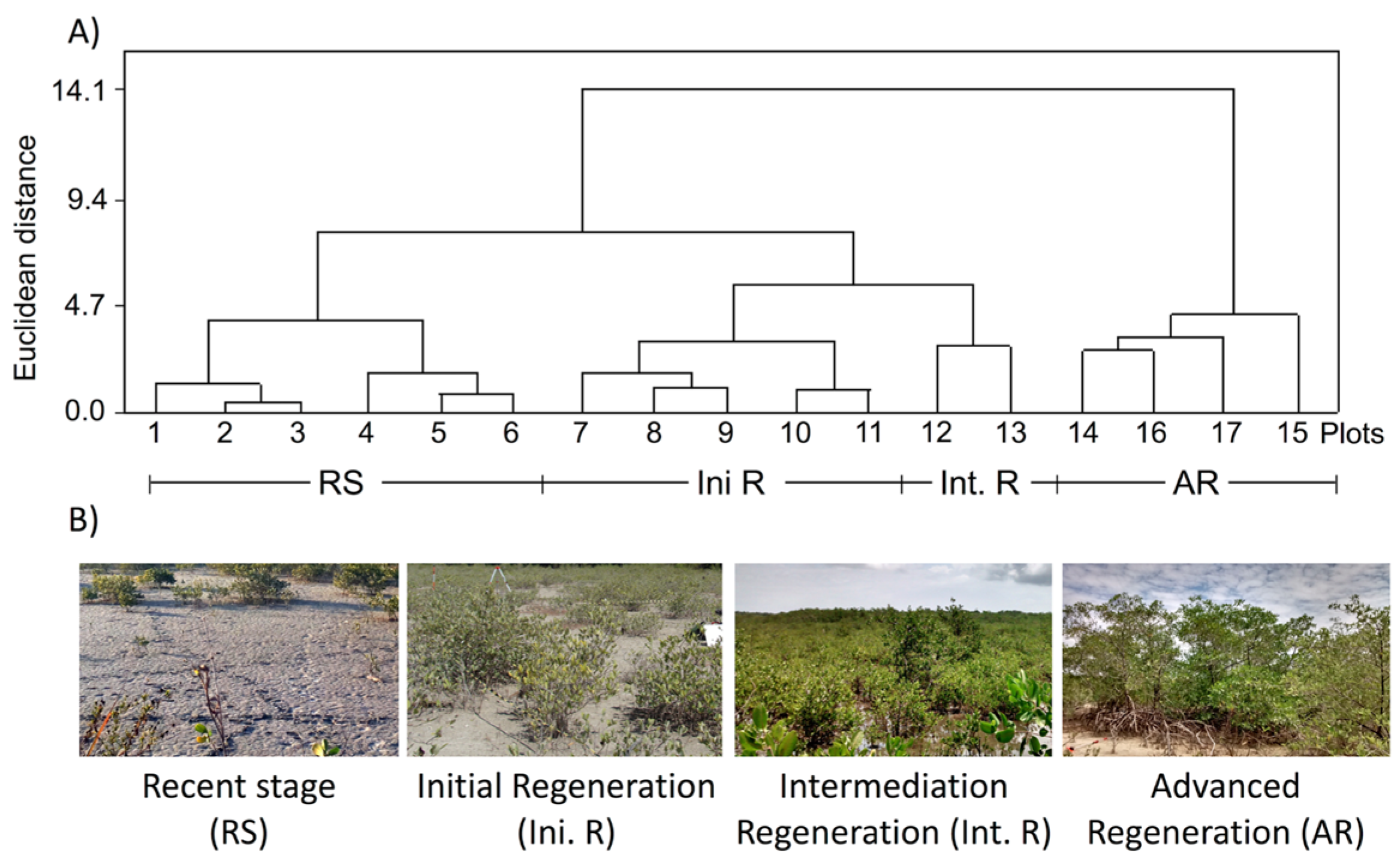
An ANOVA analysis was performed to evaluate the similarity between the four groups (recent stage, initial regeneration, intermediate regeneration and advanced regeneration) based on the average of the different structural attributes. Among these attributes, only density did not show significant differences (Table 3). The post-hoc Tukey’s test showed that BA and AGB had the most significant difference among the four groups. In Table 4, which contains the structural attributes and respective averages separated by stage, the differences between the groups are clear, especially for the attributes BA and AGB. In relation to specific composition, A. germinans and L. racemosa occur in all plots; however, A. germinans is dominant. R. mangle occurred only in the advanced regeneration stage (Group IV).
Table 3. Analysis of variance (ANOVA) of the structural parameters considering the groups formed in the cluster analysis of the plots (p > 0.05).
Structural ParametersInterceptGroup
Lorey’s HeightF43.639711.0652
p-value0.00000.0007
Mean HeightF57.887414.1051
p-value0.00000.0002
Max. HeightF58.797310.2756
p-value0.00000.0010
DBHF128.501312.0889
p-value0.00000.0005
BAF612.168780.2152
p-value0.00000.0000
BiomassF188.345336.4730
p-value0.00000.0000
DensityF26.17161.0950
p-value0.0002* 0.3861
* no significant p = 0.05.
Table 4. Structural attributes of the plots showing the formed groups.
PGroupDominant SpeciesDensityTotal DensityBasal AreaMean DBHLorey’sHeight MeanMax.Total Biomass
(ind·ha−1)(ind·ha−1)
DBH < 4 cmDBH > 4 cm(ind·ha−1)(m2·ha−1)(cm)(m)(m)(m)(kg·m−2)
1IAvicennia1600-16000.151.060.320.300.460.03
28100-81001.131.210.500.371.130.28
314,800-14,8001.451.040.490.371.040.32
413,20070013,9003.721.550.750.461.431.09
519,10040019,5005.041.630.610.471.41.43
639,90040040,3005.751.180.640.381.81.60
Group average16,11750016,3672.871.280.550.391.210.79
7IIAvicennia30,90060031,5007.261.500.850.552.372.10
814,300150015,8008.312.281.390.933.12.62
910,100160011,7008.112.582.811.914.952.69
1012,800200014,80010.432.622.632.034.783.36
117300270010,00010.983.202.431.574.553.82
Group average15,080168016,7609.022.442.021.393.952.92
12IIIAvicennia52,500120053,70014.561.631.951.184.134.35
1341003100720014.114.342.431.9645.43
Group average28,300215030,45014.342.982.191.574.074.89
14IVAvicennia13,100470017,80020.423.386.955.0810.856.50
1552003800900018.344.353.182.094.747.36
1624004300670020.895.634.923.8879.53
1716002100370020.786.9010.556.3915.1511.24
Group average55753725930020.115.076.404.369.448.66

3.3. Estimating Structural Attributes of Regenerating Mangrove Vegetation from SAR Data

The best correlation with structural attributes was found for cross-polarization backscatter (Table 5). The VV polarization obtained low and inverse correlations, which can be related to the lower stature of the vegetation. This result may occur because we are working with a regenerating forest where horizontal scattering predominates and causes the opposite of what was described by van der Sanden [24].
Table 5. Correlation coefficient between structural attributes and backscattering of the Radarsat-2 image FQ5. The highest correlation coefficient values are highlighted (p < 0.05).
Lorey’s HeightMean HeightMax HeightDBHBasal AreaTotal Biomass
(m)(m)(m)(cm)(m2·ha−1)(kg·ha−1)
β°HH0.200.170.220.220.150.18
β°HV0.560.600.540.610.620.64
β°VH0.710.700.690.670.620.68
β°VV−0.74−0.12−0.08−0.14−0.17−0.13
σ°HH0.560.530.560.520.470.55
σ°HV0.510.600.490.580.620.58
σ°VH0.770.790.750.730.680.72
σ°VV−0.03−0.07−0.02−0.16−0.14−0.12
γHH0.200.240.230.190.120.12
γHV0.350.420.370.400.590.45
γVH0.580.610.590.550.660.59
γVV0.030.010.040.00−0.05−0.04
Different functions were fitted to the set of variables with significant correlation coefficients. Table 6 shows that the best fit of the regression function is linear and best with the σ°VH backscattering.
Table 6. Models that showed higher r2 values in the three radar attributes with VH polarization as an explanatory variable (p > 0.05).
Lorey’s HeightMean HeightMaximum Height
r2β1 (p)Fpr2β1 (p)Fpr2β1 (p)Fp
σ°VHLIN0.590.00021.9090.000LIN0.630.00025.2370.000LIN0.570.00019.5870.000
β°VHLIN0.500.00214.7950.002LIN0.490.00214.6120.002LIN0.480.00213.6810.002
γVHEXP0.410.00610.2650.006EXP0.430.00411.420.004EXP0.370.0098.9580.009
DBHBasal AreaBiomass
r2β1 (p)Fpr2β1 (p)Fpr2β1 (p)Fp
σ°VHLIN0.530.00116.9790.000LIN0.460.00312.9500.003LIN0.520.00116.4300.001
β°VHLIN0.440.00311.9870.000LIN0.390.0089.4660.008LIN0.460.00312.5720.003
γVHEXP0.350.0137.9440.013LIN0.440.01411.6710.004LIN0.350.0128.0730.012
Multiple linear regression models were subsequently fitted to potentially increase the predictive power of the regressions. The multicolinearity between the independent variables that compose these models was verified by VIF (variance inflation value), which resulted in the values of 1.41, 1.13 and 1.27 for σ°HH, σ°VH, and σ°VV, respectively. These values are below the limit value of 10 indicated by Neter et al. [50]. The parameters of these models are provided in Table 7.
The variable σ°VV3, Table 7) was not statistically significant in the regression model of the attribute maximum height previously described. Therefore, it is possible that the vertical components of the vegetation are not sufficiently developed to interact with microwaves in the VV polarization.
In the residual analysis, the models met the assumptions proposed by Neter et al. [50]. With the PRESS values, the models produced adequate values, especially those for horizontal structures, which showed a better predictive ability in the fit regression function with an emphasis on the DBH model (Table 8).
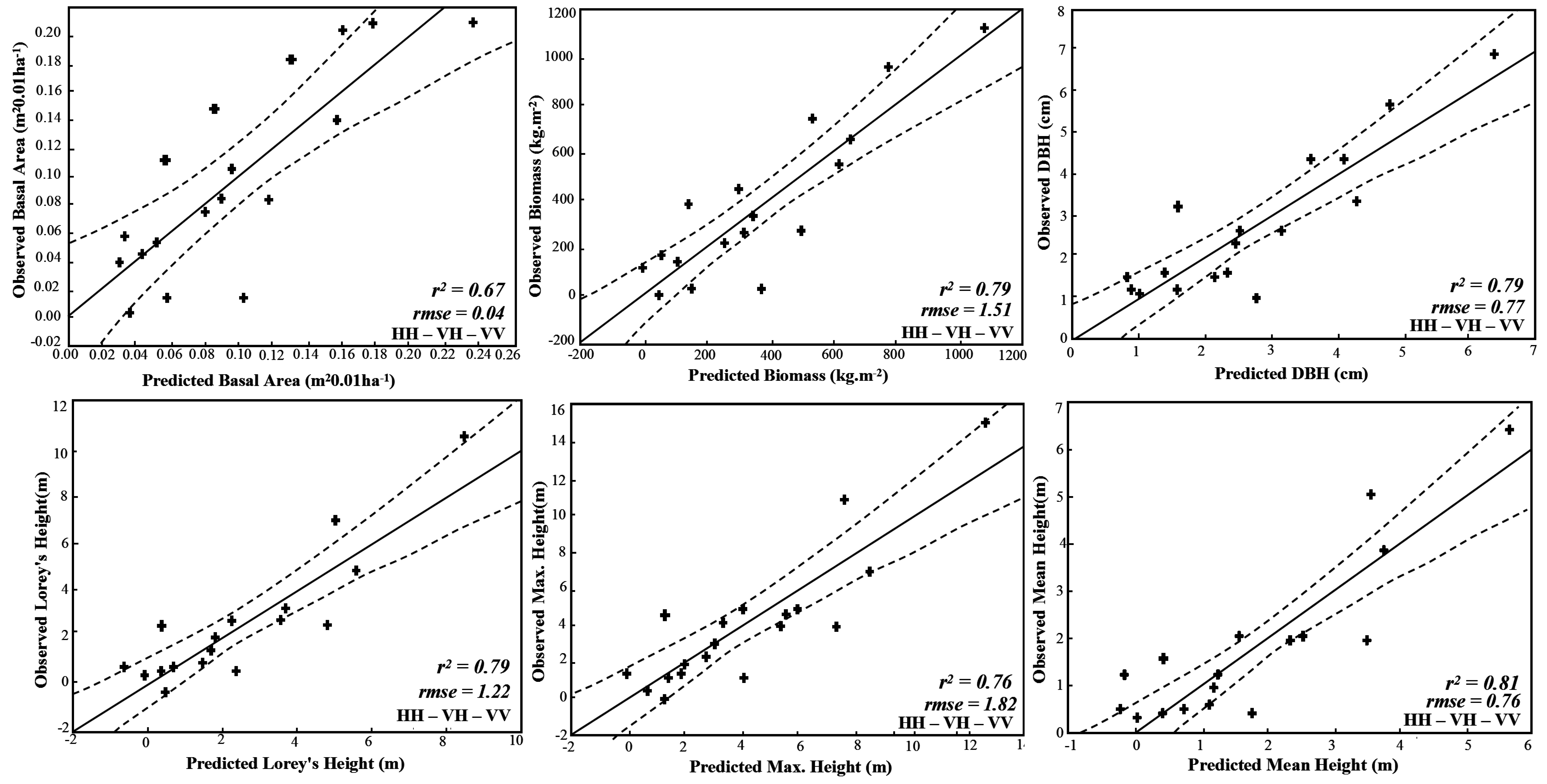
Although the maximum height model was simpler (Figure 4), the average height model had a higher predictive ability based on the RMSE value. For the estimation of the horizontal structure, the model for DBH had the best predictive ability, although other models were satisfactory (Figure 4). When comparing the verified modeling methods, r2 values increase with the introduction of σ°HH and σ°VV backscattering as independent variables. The explanatory power increased between 11% and 19% for the models of height estimation and between 20% and 27% for the models of estimation of horizontal structure and AGB. The RMSE values decreased with the inclusion of these variables; the PRESS values also decreased. This indicates that these models should be chosen instead of the simple regression models [51].
Table 7. Parameters of the simple and multiple regression models and σ°HH, σ°VH, and σ°VV backscattering that compose the independent variables.
Lorey’s HeightMean HeightMax. Height
SimpleMultipleSimpleMultipleSimpleMultiple
r20.590.790.630.810.570.760.68
β00.020−0.5150.049−0.1910.8170.010−0.593
β1 (σ°HH)-0.502-0.468-0.5050.636
p-0.006-0.007-0.0080.001
β2 (σ°VH)0.7700.6410.7920.6770.7530.6214.323
p0.0000.0000.0000.0000.0000.0010.045
β3 (σ°VV)-−0.329--0.356-−0.318-
p-0.040-0.022-0.059-
ε1.78941.3961.12480.8702.59232.0822.312
F21.90915.86925.23718.08719.58713.54114.743
p0.0000.0000.0000.0000.0000.0000.000
DBHTotal BiomassBasal Area
SimpleMultipleSimpleMultiple* Simple** SimpleMultiple
r20.530.790.520.790.460.500.67
β00.4731.03387.05639.0090.0210.0070.038
β1 (σ°HH)-0.5311278-0.472
p-0.0040.003-0.027
β2 (σ°VH)0.7290.6040.72372790.6810.6140.571
p0.0010.0010.0010.0010.0030.0010.005
β3 (σ°VV)-−0.465−868-−0.422
p-0.0070.009-0.035
ε1.21930.882234.83168.1100.05340.05140.045
F16.97916.03316.43016.10912.95015.1508.788
p0.0010.0000.0010.0000.0030.0010.002
Legend: r2 = determination coefficient; β0 = line intercept; β1,2,3 = line inclination; ε = random error, F = Fischer test for total variance model, * σ°VH (5 × 5) = independent variable, and ** γ °VH (3 × 3) = independent variable.
Table 8. PRESS values and SQR difference percentage.
MultipleSimple
AttributePRESSSQR%PRESSSQR%
Lorey’s Height53.5925.3552.6979.4748.0339.56
Mean Height18.509.8446.8228.6118.9833.68
Max. Height140.5174.8346.74162.38100.8037.92
DBH15.6910.1235.5329.6922.3024.89
Total Biomass639,023367,40842.501,072,887827,19722.90
* Basal Area0.040.0339.800.0520.04317.47
** Basal Area---0.0490.04019.26
* σ°VH (5 × 5): independent variable; ** γ VH (3 × 3): independent variable.
Figure 4. Plots of the observed values against the predicted values, with respective r2 and RMSE values.
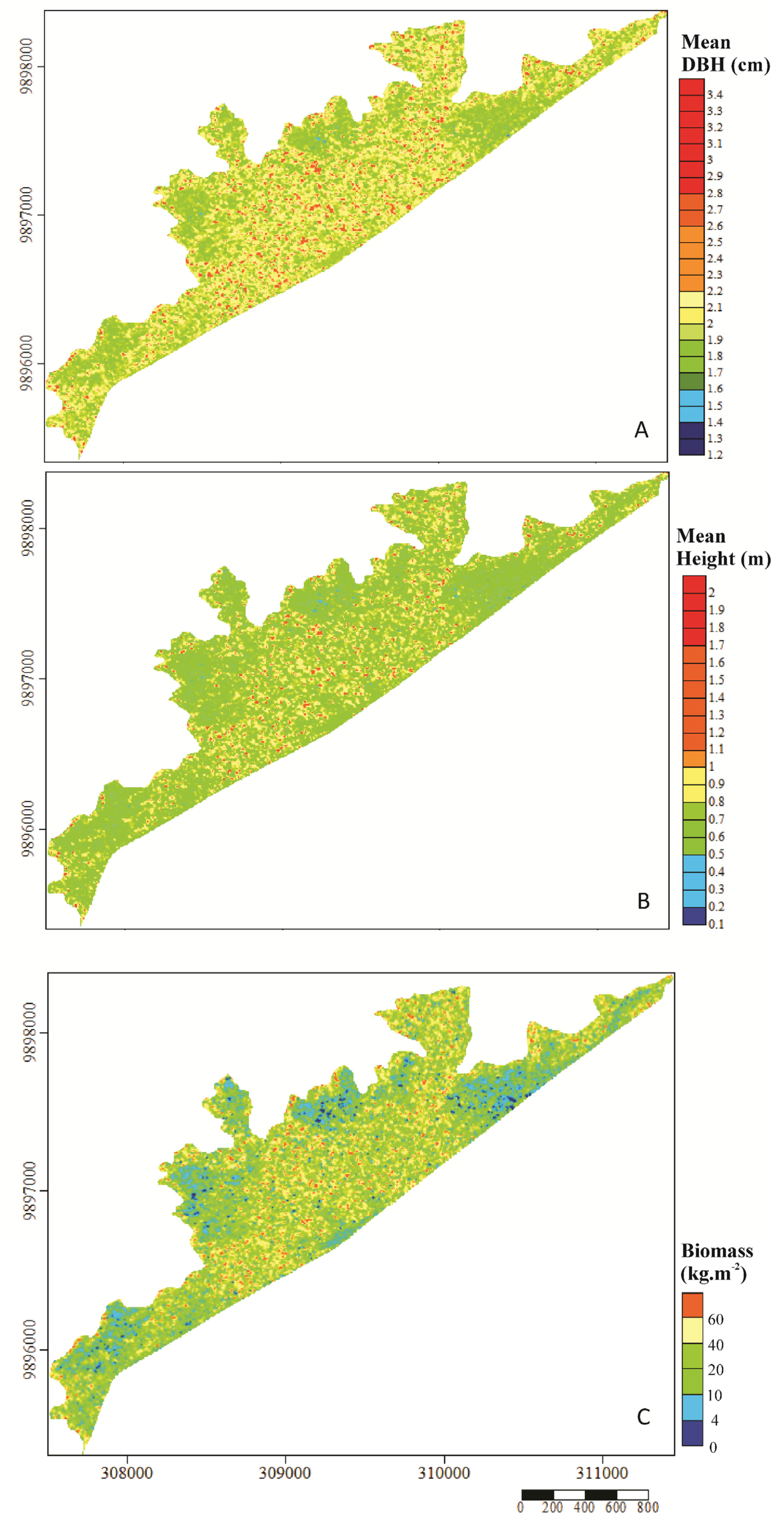
Remotesensing 07 15873 g004
Figure 5. Estimation map: (A) average DBH (cm) and (B) average height (m) and (C) total biomass (kg·m−2) based on the backscattering values through their multiple regression functions.
Remotesensing 07 15873 g005
The fitted regression models were developed and validated, and then applied to the backscattering values from the Radarsat-2 FQ5 image to generate maps of DBH, average height and AGB (Figure 5). The values shown in the average DBH map ranged between 1.2 and 3.3 cm, which is consistent with the data measured in the field, in which only four sample units had values above 3.3 cm. The map showed a few regions with DBH lower than 1.6 cm, and most of the individuals with greater DBH were in the central portion of the map and ranged from 2 to 3.3 cm. The applied parameter was the average DBH, whose model RMSE was 0.77 cm; because it is a regenerating mangrove region, the amplitude of variation of this measurement is high as a result of the structural heterogeneity. The average height ranged from 0.2 to 1.9 m and is considered consistent with the values measured in the field, especially when considering the RMSE of the model, which was 0.76 m; there were only three plots outside of this height range.
The total AGB map showed a large value variation between 0 and 60 kg·m−2. These values include all AGB measured in the field. Zero represents areas without vegetation with exposed tidal flats. The more frequent values are between 10 and 40 kg·m−2. This model seemed to overestimate AGB, which is most likely a result of double-bounce scattering.

4. Conclusions

The regenerating mangrove vegetation showed structural heterogeneity with a wide range of structural parameter variation, and the BA was the best variable to distinguish the regeneration stages. Four stages were differentiated into groups: recent stage (Group I), initial regeneration (Group II), intermediate regeneration (Group III) and advanced regeneration (Group IV). The dominant species in the greatest number was Avicennia germinans. The species Laguncularia racemosa had the lowest occurrence in the four groups and the species Rhizophora mangle was only found in the advanced regeneration group. The equation used to calculate AGB reflected the high range of variation between the four groups and can be considered adequate. Particularly, linear sigma backscattering σ° showed the strongest and most significant correlation with the structural data from the regenerating mangrove vegetation, especially in the VH cross-polarization.
The multiple regression model with the σ°HH, σ°VH and σ°VV polarization showed high predictive capacity for the variables’ average height (r2 = 0.81), DBH (r2 = 0.79) and AGB (r2 = 0.79), which permitted the generation of maps of these vegetation attributes. Therefore, DBH and average height maps exhibit values commensurate with those observed in the fieldwork. The central region of the study site showed the highest values of DBH and average height, and consequently, this region showed the highest values of total AGB. The AGB measured in the field presented a high correlation with Radarsat-2 backscattering. Finally, this study provided important new insights into the interpretation of multi-polarized Radarsat-2 images, which showed to be adequate for the estimation of vegetation attributes in areas of mangrove regeneration. Additional research will explore the influence of full polarimetric C-band RADARSAT-2 data (decomposition and polarimetric response), involving all successional stages of mangrove vegetation.

Acknowledgments

We would like to acknowledge the financial support and field assistance provided by the Coordenação de Aperfeiçoamento de Pessoal de Nível Superior (CAPES-Brazil) and Conselho Nacional de Desenvolvimento Científico e Tecnológico (CNPq-Brazil). We would also like to acknowledge support provided by Universidade Federal do Pará and Fundação de Amparo e Desenvolvimento da Pesquisa - FADESP. Thanks are also extended to the Canadian Spatial Agency, which provided Radarsat-2 images from the “Science and Operational Application Research (SOAR)” project, and Santiago & Cintra, who provided the RapidEye images. Simard is supported from the NASA LCLUC program. We would also like to thank Afonso Quaresma and Edson Pereira for the fieldwork support. Finally, we would also like to thank the reviewers of this paper and their valuable contributions towards refining the manuscript.

Author Contributions

Michele Cougo conducted the image processing, analysis and fieldwork, and wrote the first draft of manuscript. Pedro Souza-Filho designed the remote sensing research approach and supervised image processing and analysis. Marcus Fernandes designed and supervised the collection of structural mangrove data. João Santos supervised structural mangrove data analysis. Maria Abreu and Nascimento Jr. conducted fieldwork to collecte and analyze geo-referenced structural mangrove data. Marc Simard helped with structural parameters and biomass estimation. All authors read and approved the final version of the manuscript.

Conflicts of Interest

The authors declare no conflict of interest.

References

  1. Kathiresan, K.; Bingham, B.L. Biology of mangroves. In Advances in Marine Biology; University of New Hampshire: Durham, NH, USA, 2001. [Google Scholar]
  2. Hogarth, P.J. The Biology of Mangroves and Seagrasses; Oxford University Press: New York, NY, USA, 1999. [Google Scholar]
  3. Alongi, D.M. Present state and future of the world’s mangrove forests. Environ. Conserv. 2002, 29, 331–349. [Google Scholar] [CrossRef]
  4. Lugo, A.E.; Snedaker, S.C. The ecology of mangroves. Ann. Rev. Ecol. Syst. 1974, 5, 39–64. [Google Scholar] [CrossRef]
  5. Spalding, M.; Blasco, F.; Field, C.D. World Mangrove Atlas; International Society for Mangrove Ecosystems: Tresaith, Cardigan, UK, 1997. [Google Scholar]
  6. Soares, M.L.G.; Schaeffer-Novelli, Y. Above-ground biomass of mangrove species. I. Analysis of models. Estuar. Coast. Shelf Sci. 2005, 65, 1–18. [Google Scholar] [CrossRef]
  7. Aheto, D.W.; Aduomih, A.A.O.; Obodai, E.A. Structural parameters and above-ground biomass of mangrove tree species around the Kakum river estuary of Ghana. Ann. Biol. Res. 2011, 2, 504–514. [Google Scholar]
  8. Castelan-Estrada, M.; Vivin, P.; Gaudillère, J.P. Allometric Relationships to estimate seasonal above-ground vegetative and reproductive biomass of vitis vinifera L. Ann. Bot. 2002, 89, 401–408. [Google Scholar] [CrossRef] [PubMed]
  9. Gehring, C.; Park, S.; Denich, M. Close relationship between diameters at 30 cm height and at breast height (DBH). Acta Amaz. 2008, 38, 71–76. [Google Scholar] [CrossRef]
  10. Ross, M.S.; Ruiz, P.L.; Telesnicki, G.J.; Meeder, J.F. Estimating above-ground biomass and production in mangrove communities of Biscayne National Park, Florida (USA). Wetl. Ecol. Manag. 2001, 9, 27–37. [Google Scholar] [CrossRef]
  11. Komiyama, A.; Ong, J.E.; Poungparn, S. Allometry, biomass, and productivity of mangrove forests: A review. Aquat. Bot. 2008, 89, 128–137. [Google Scholar] [CrossRef]
  12. Chave, J.; Andalo, C.; Brown, S.; Cairns, M.A.; Chambers, J.Q.; Eamus, D.; Fölster, H.; Fromard, F.; Higuchi, N.; Kira, T.; et al. Tree allometry and improved estimation of carbon stocks and balance in tropical forests. Oecologia 2005, 145, 87–99. [Google Scholar] [CrossRef] [PubMed]
  13. Comley, B.W.T.; McGuinness, K.A. Above- and below-ground biomass, and allometry of four common northern Australian mangroves. Aust. J. Bot. 2005, 53, 431–436. [Google Scholar] [CrossRef]
  14. Food and Agriculture Organization. The World’s Mangroves 1980–2005; FAO Forestry Paper; FAO: Roma, Italy.
  15. De Menezes, M.P.M.; Berger, U.; Mehlig, U. Mangrove vegetation in Amazonia: A review of studies from the coast of Pará and Maranhão States, north Brazil. Acta Amaz. 2008, 38, 403–420. [Google Scholar] [CrossRef]
  16. Henderson, F.M.; Lewis, A.J. Radar detection of wetland ecosystems: A review. Int. J. Remote Sens. 2008, 29, 5809–5835. [Google Scholar] [CrossRef]
  17. Kovacs, J.M.; Vandenberg, C.V.; Wang, J.; Flores-Verdugo, F. The use of multipolarized spaceborne SAR backscatter for monitoring the health of a degraded mangrove forest. J. Coast. Res. 2008, 241, 248–254. [Google Scholar] [CrossRef]
  18. De Souza Pereira, F.R.; Kampel, M.; Cunha-Lignon, M. Mapping of mangrove forests on the southern coast of São Paulo, Brazil, using synthetic aperture radar data from ALOS/PALSAR. Remote Sens. Lett. 2012, 3, 567–576. [Google Scholar] [CrossRef]
  19. Simard, M.; Grandi, G.D.; Saatchi, S.; Mayaux, P. Mapping tropical coastal vegetation using JERS-1 and ERS-1 radar data with a decision tree classifier. Int. J. Remote Sens. 2002, 23, 1461–1474. [Google Scholar] [CrossRef]
  20. Simard, M.; Rivera-Monroy, V.H.; Mancera-Pineda, J.E.; Castañeda-Moya, E.; Twilley, R.R. A systematic method for 3D mapping of mangrove forests based on Shuttle Radar Topography Mission elevation data, ICEsat/GLAS waveforms and field data: Application to Ciénaga Grande de Santa Marta, Colombia. Remote Sens. Environ. 2008, 112, 2131–2144. [Google Scholar] [CrossRef]
  21. Souza-Filho, P.W.M.; Paradella, W.R. Recognition of the main geobotanical features along the Bragança mangrove coast (Brazilian Amazon Region) from Landsat TM and RADARSAT-1 data. Wetl. Ecol. Manag. 2002, 10, 123–132. [Google Scholar]
  22. Souza-Filho, P.W.M. Costa de manguezais de macromaré da Amazônia: Cenários morfológicos, mapeamento e quantificação de áreas usando dados de sensores remotos. Rev. Bras. Geofísica 2005, 23, 427–435. [Google Scholar] [CrossRef]
  23. Ranson, K.J.; Sun, G. Mapping biomass of a northern forest using multifrequency SAR data. IEEE Trans. Geosci. Remote Sens. 1994, 32, 388–396. [Google Scholar] [CrossRef]
  24. Van der Sanden, J.J. Radar Remote Sensing to Support Tropical Forest Management; Tropenbos Guyana Series; Tropenbos—Guyana Programme: Georgetown, Guyana, 1997. [Google Scholar]
  25. Kovacs, J.M.; Vandenberg, C.V.; Flores-Verdugo, F. Assessing fine beam RADARSAT-1 backscatter from a white mangrove (Laguncularia racemosa (Gaertner)) canopy. Wetl. Ecol. Manag. 2006, 14, 401–408. [Google Scholar] [CrossRef]
  26. Mougin, E.; Proisy, C.; Marty, F.; Fromard, F.; Puig, H.; Betoulle, J.L.; Rudant, J.P. Multifrequency and multipolarization radar backscattering from mangrove forests. IEEE Trans. Geosci. Remote Sens. 1999, 37, 94–102. [Google Scholar] [CrossRef]
  27. Proisy, C.; Mougin, E.; Fromard, F.; Trichon, V.; Karam, M.A. On the influence of canopy structure on the radar backscattering of mangrove forests. Int. J. Remote Sens. 2002, 23, 4197–4210. [Google Scholar] [CrossRef]
  28. Proisy, C.; Couteron, P.; Fromard, F. Predicting and mapping mangrove biomass from canopy grain analysis using Fourier-based textural ordination of IKONOS images. Remote Sens. Environ. 2007, 109, 379–392. [Google Scholar] [CrossRef]
  29. Simard, M.; Zhang, K.; Rivera-Monroy, V.H.; Ross, M.S.; Ruiz, P.L.; Castañeda-Moya, E.; Twilley, R.R.; Rodrigues, E. Mapping height and biomass of mangrove forests in everglades National Park with SRTM elevation data. Photogramm. Eng. Remote Sens. 2006, 72, 299–311. [Google Scholar] [CrossRef]
  30. Kovacs, J.M.; Jiao, X.; Flores-de-Santiago, F.; Zhang, C.; Flores-Verdugo, F. Assessing relationships between Radarsat-2 C-band and structural parameters of a degraded mangrove forest. Int. J. Remote Sens. 2013, 34, 7002–7019. [Google Scholar] [CrossRef]
  31. Kovacs, J.M.; Lu, X.X.; Flores-Verdugo, F.; Zhang, C.; Flores de Santiago, F.; Jiao, X. Applications of ALOS PALSAR for monitoring biophysical parameters of a degraded black mangrove (Avicennia germinans) forest. ISPRS J. Photogramm. Remote Sens. 2013, 82, 102–111. [Google Scholar] [CrossRef]
  32. Rubén, L.; Claudio, S.; Marcelo, C.; Uta, B.; Marion, G. Implications of mangrove dynamics for private and use in bragança, north Brazil: A case study. J. Coast. Conserv. 2002, 8, 97–102. [Google Scholar] [CrossRef]
  33. Nascimento, W.R.; Souza-Filho, P.W.M.; Proisy, C.; Lucas, R.M.; Rosenqvist, A. Mapping changes in the largest continuous Amazonian mangrove belt using object-based classification of multisensor satellite imagery. Estuar. Coast. Shelf Sci. 2013, 117, 83–93. [Google Scholar] [CrossRef]
  34. Fisch, G.; Marengo, J.A.; Nobre, C.A. Uma revisão geral sobre o clima da Amazônia. ACTA Amaz. 1998, 28, 101–126. [Google Scholar] [CrossRef]
  35. Monteiro, M.C.; Pereira, L.C.C.; Oliveira, S.M.O. Morphodynamic changes of a macrotidal sand beach in the brazilian Amazon coast (Ajuruteua-Pará). J. Coast. Res. Issue 56 2009, 56, 103–107. [Google Scholar]
  36. Souza-Filho, P.W.M.; Lessa, G.C.; Cohen, M.C.; Costa, F.R.; Lara, R.J. The Subsiding Macrotidal Barrier Estuarine System of the Eastern Amazon Coast, Northern Brazil. In Geology of Brazilian Coastal Barriers; Dillenburg, S.F., Hesp, P.A., Eds.; Springer: New York, NY, USA, 2009; p. 220. [Google Scholar]
  37. Souza-Filho, P.W.M.; El-Robrini, M. Geomorphology of the Bragança Coastal zone, northeastern Pará State. Rev. Bras. Geociê. 2000, 30, 518–522. [Google Scholar]
  38. Menezes, M.P.M.; Mehlig, U. Floristics and forest structure—Mangrove vegetation of the Caeté Estuary. In Mangrove Dynamics and Management in North Brazil; Saint-Paul, U., Schneider, H., Eds.; Springer: Berlin, Germany, 2010. [Google Scholar]
  39. Mehlig, U.; Menezes, M.P.M.; Reise, A.; Schories, D.; Medina, E. Mangrove vegetation of the Caeté Estuary. In Mangrove Dynamics and Management in North Brazil; Saint-Paul, U., Schneider, H., Eds.; Springer: Berlin, Germany, 2010. [Google Scholar]
  40. Instituto Nacional de Meteorologia (INMET). Brazilian Institute of Meteorology: Precipitation Data. Available online: http://www.inmet.gov.br/portal/ (accessed on 31 January 2014).
  41. Diretoria de Hidrografia e Navegação (DHN). Brazilian Navy: Tide Prediction. Available online: http://www.mar.mil.br/dhn/chm/box-previsao-mare/tabuas/ (accessed on 31 January 2014).
  42. Toutin, T. Intégration de données multi-source: Comparaison de méthodes géométriques et radiométriques. Int. J. Remote Sens. 1995, 16, 2795–2811. [Google Scholar] [CrossRef]
  43. Lee, J.-S.; Grunes, M.R.; de Grandi, G. Polarimetric SAR speckle filtering and its implication for classification. IEEE Trans. Geosci. Remote Sens. 1999, 37, 2363–2373. [Google Scholar]
  44. Woodhouse, I. Introduction to Microwave Remote Sensing; Taylor & Francis: London, UK, 2004. [Google Scholar]
  45. Cintrón, G.M.; Schaeffer-Novelli, Y. The Mangrove Ecosystem: Research Methods; S.C. Snedaker and J.G. Snedaker: Paris, France, 1984. [Google Scholar]
  46. Soares, M.L.G. Estrutura vegetal e grau de perturbação dos manguezais da Lagoa da Tijuca, Rio de Janeiro, RJ, Brasil. Rev. Bras. Biol. 1999, 59, 503–515. [Google Scholar] [CrossRef]
  47. Avery, T.E.; Burkhart, H.E. Forest Measurements; McGraw-Hill: New York, NY, USA, 2001. [Google Scholar]
  48. Tukey, J.W. The Problem of Multiple Comparisons; Princeton University: Princeton, NJ, USA, 1953. [Google Scholar]
  49. Fromard, F. Structure, above-ground biomass and dynamics of mangrove ecosystems: New data from French Guiana. Oecologia 1998, 115, 39–53. [Google Scholar] [CrossRef]
  50. Neter, J. Applied Linear Statistical Models; IRWIN: New York, NY, USA, 1996. [Google Scholar]
  51. Rencher, A.C.; Schaalje, G.B. Linear Models in Statistics; John Wiley & Sons: Hoboken, NJ, USA, 2008. [Google Scholar]

