1. Introduction
Developing geometric documentation is one of the most basic tasks in the fields of conservation policy and management of cultural heritage objects. 3D documentation is a prerequisite of conservation or restoration work on historical objects and sites. Development of specific documentation such as high-resolution orthoimages is necessary at all stages of conservation works.
Orthoimages are attractive for archaeological and architectural documentation, as they offer a combination of geometric accuracy and visual quality [
1], and can also be applied to different measuring techniques.
Integration of Terrestrial Laser Scanning (TLS) and image-based data can lead to better results [
2,
3]. Despite many advantages, the TLS technique also has a lot of limitations; for example,it is not possible to acquire sharp edges, poor quality or reflective surfaces,
etc. Another issue is caused by areas with obstacles or hidden points. In this case, in order to fill in the blind spots, more stations are required. Laser scanners are currently integrated with low-resolution cameras. In many cases, it is recommended to use additional, high-resolution images in order to produce the required orthoimages. However, in many cases of TLS data utilization, the additional information is an intensity value, applied by conservators to evaluate the conditions of the surfaces of given historical objects [
4].
3D modelling systems have now also been dynamically developed; they are based on digital images and utilize Computer Vision (CV) algorithms to automatically create 3D models [
5,
6,
7,
8,
9]. Tools which utilize the Structure from Motion (SfM) approach are also being developed. CV algorithms allow for automatic creation of textured 3D surface models based on a sequence of images, without any prior knowledge concerning objects or the camera. Developed software tools also allow generation of orthoimages [
5,
7,
10].
Integration of TLS and SfM technologies therefore becomes an alternative in many works on complicated architectural objects [
6,
11]. Although new imaging systems have been dynamically developed, many problems inherent in the integration of TLS and digital images are still waiting to be solved [
12]. The possibilities of using digital technologies in the conservation process have been widely analysed. However, solutions to automate the generation of cultural-heritage-object documentation are still lacking. In many cases scanning data on cultural heritage objects exist already; it is only necessary to acquire high-resolution orthoimages with the use of additional, “free-hand” images.
The authors of this paper closely co-operate with the Museum of King John III’s Palace in Wilanów in conservation works, as well as in other projects. Development of metric documentation of complicated historical objects requires implementation of an automated technological process. Based on this experience the orthoimage generation process has been automated with the use of terrestrial laser-scanning data and “arbitrary” high-resolution images.
2. Problem Statement
This paper focuses on generating orthoimages through automatic integration of TLS data with “free-hand” images. In the past, many cultural heritage objects were measured with the use of scanners without digital cameras; the results were point cloud with intensity values (near infrared) and transformed to the orthoimages. Due to the spectral range in which such an orthoimage is recorded, it seems to have a low visual contrast. Therefore, it is necessary, in many cases, to supplement the data with digital images in order to generate RGB orthoimages (in natural colours).
When orthoimages are generated it is important to settle two basic issues: accuracy, and resolution [
13]. In this case integration of a TLS point cloud and digital images improves the geometric and radiometric quality of generated orthoimages [
5,
6,
7,
8,
11,
14,
15].
Problems can also result from the nature of close-range measurements,
i.e., the proximity of objects of complex geometry [
1]. Such difficulties have been widely discussed in the context of “true-ortho” generation for architectural objects, where orthoimages are the basic tool for documentation [
16,
17].
Many publications have demonstrated the role of TLS data in improving the accuracy and automation level [
16,
18]. Unfortunately, software for full automatic generation of orthoimages does not yet exist.
Modern terrestrial scanners are equipped with digital cameras of low resolution, and measurements are performed from the same position. Thus, scans and images are automatically integrated. However, in order to obtain RGB orthoimages of sufficient quality, it is necessary to use images of higher resolution, acquired independently of the scanner station [
16]. Therefore, a separate issue concerns the integration of TLS data with “free-hand” images of higher resolution [
19,
20].
It is necessary to create procedures of integration of a TLS point cloud and “arbitrary” acquired images in order to generate a high-resolution orthoimage that will improve the quality of the point clouds and resolution texture of 3D models. Achieving geometric accuracy and visual quality is time consuming; the process needs to be performed manually or semi-automatically.
The first experiments testing the presented approach were discussed in [
18]. These initial experiments were performed using the unmodified Hough transform for uncomplicated architectural objects, creating one plane of smaller depth.
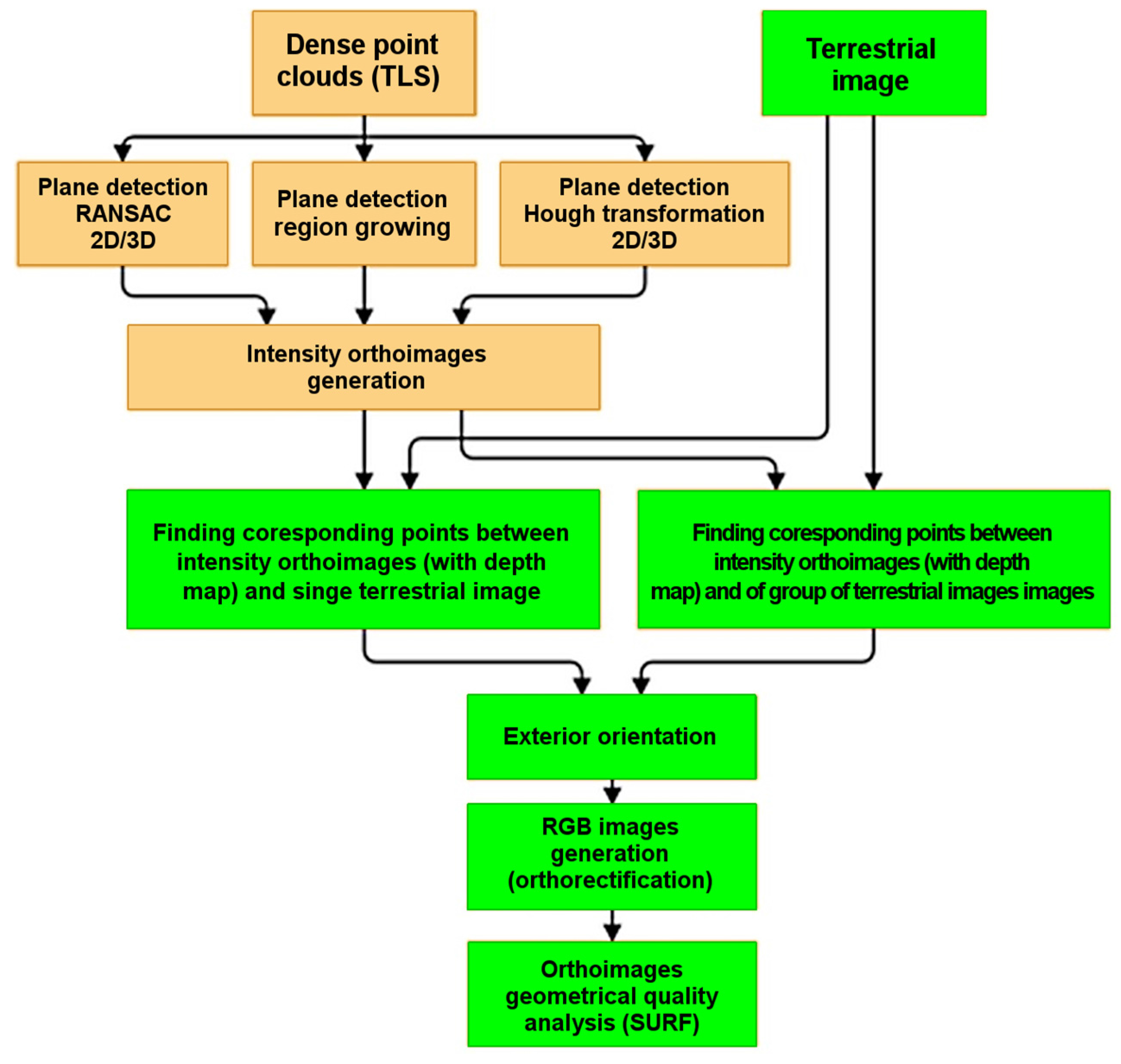
The authors of this paper have developed original tools that automate the process of RGB image generation.Experiments performed to this end are presented in
Figure 1.
Figure 1.
Diagram of the performed experiments.
Figure 1.
Diagram of the performed experiments.
The following issues are discussed in the paper:
detection of horizontal and vertical planes from the so-called “raw point clouds” with the use of the processed Hough transform;
checking the accuracy of plane matching and setting the points buffer for creation of the Digital Surface Model (DSM) of an object and the intensity image;
DSM generation in the rectangular grid (GRID) form, and generation of intensity orthoimages with a depth map;
orientation of terrestrial images based on orthoimages with the assigned depth map using the utilize Scale Invariant Feature Transform (SIFT) algorithm;
quality control of matching images in relation to the point clouds/an orthoimage with the depth map;
orthorectification and mosaicking of terrestrial images based on the previously generated DSM;
quality control of the coloure orthoimages (Red Green Blue—RGB) based on the Speeded-Up Robust Features (SURF) algorithm and the intensity orthoimage.
3. Methodology
Utilization of terrestrial laser-scanning data requires consideration of the specifics of data recording.
3.1. Specifics of TLS Data
Data are recorded in the polar system, R,
ω,
φ, which causes deformation of straight lines (
Figure 2). The point cloud recorded by the scanner contains points located on different planes (on the floor, on the ceiling, and, as in the discussed case, on the walls); therefore, it is necessary to filter points located on the plane of interest (again, the wall in the discussed case). Due to different disturbances, points determined by the scanner are not directly located on the reflecting surface. As shown by
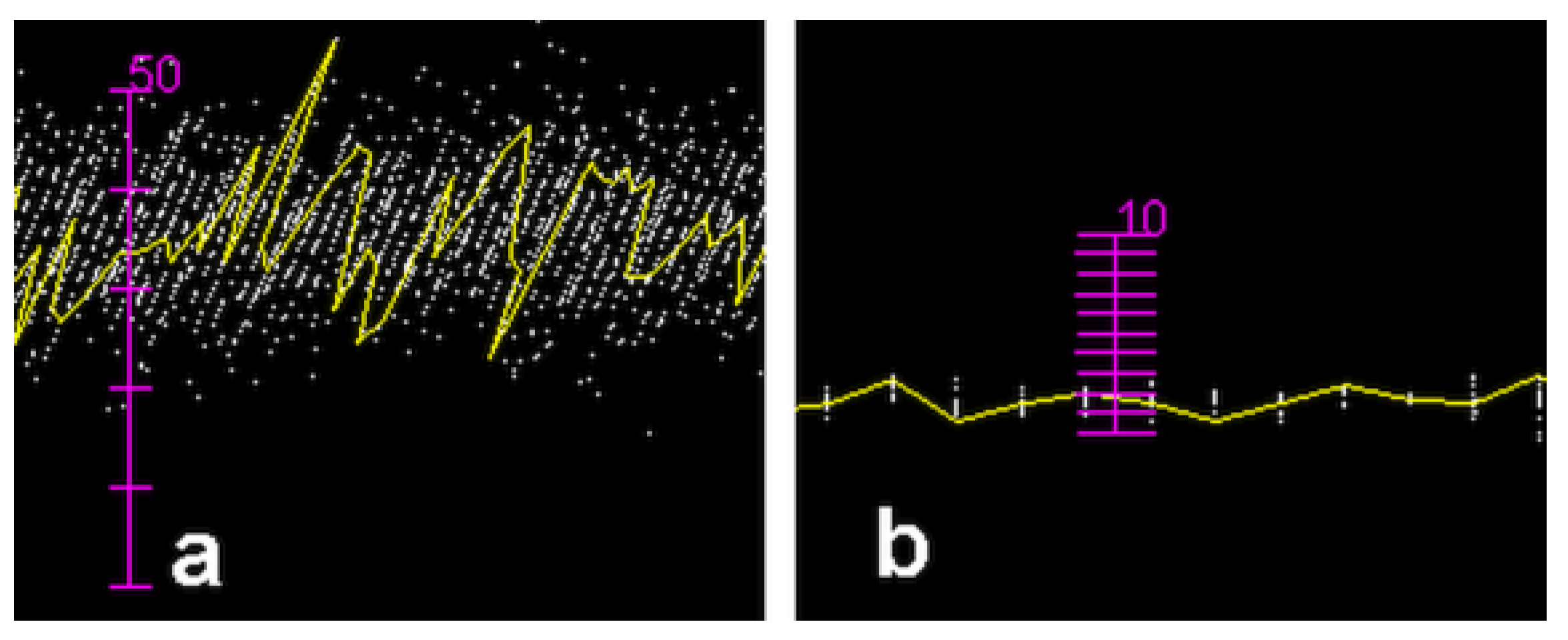
Figure 3, the distance measurement error (the scanner produces data in the polar system) as well as the laser’s light incidence angle causes points to be located inside certain cuboids (not on the plane). The depth of these cuboids depends on the scanner’s technical specifications (wavelength, modulation type, spot diameter, radiation power), as well as on the properties of the reflecting surface. Differences can emerge from scanner type (different companies have differing amounts of experience), as well as the surface structure: for example,
Figure 3a shows a fabric, whose threads could cause multiple reflections; on the other hand, and
Figure 3b shows a smoothly plastered and painted wall.
Figure 2.
Data acquired by the ZFS 5003 scanner: (a) an image of the reflectance level in the ω, φ polar system; (b) in the rectangular XZ (rotated) system; colour lines present successive rows and columns of source data.
Figure 2.
Data acquired by the ZFS 5003 scanner: (a) an image of the reflectance level in the ω, φ polar system; (b) in the rectangular XZ (rotated) system; colour lines present successive rows and columns of source data.
Figure 3.
The “thickness” of the point cloud for data recorded by the (a) Z+F 5003 scanner for a wall covered with fabric and (b) by the Z+FS 5006 scanner for the painted wall. The yellow line presents the “row” of the scanner data (mm).
Figure 3.
The “thickness” of the point cloud for data recorded by the (a) Z+F 5003 scanner for a wall covered with fabric and (b) by the Z+FS 5006 scanner for the painted wall. The yellow line presents the “row” of the scanner data (mm).
Even in the case of explicit classification of points, the thickness of the cloud and noises can influence the plane determination.
As can be seen, the properties of TLS point clouds require the use of methods resistant to gross errors. Three methods (with variants) were selected and tested: RANSAC, region-growing, and Hough transform.
3.2. Plane Equations
The plane equation in space can be described in different ways, but the general form of the equation is Equation (1):
or, in the vector form: unit length normal vector
and
r = distance from origin.
The normal vectorcan be determined from Equation (2):
and the distance from origin from Equation (3):
where
are the coordinates of a point lying on the plane.
Since vertical and horizontal planes are important for the purposes of documentation, the ranges of the permitted values of the coefficients in the above equations may be limited. For horizontal planes (i.e., floors and ceilings) it can be assumed that C ≈ 0 or ϕ ≈ ±90°, and for vertical planes (i.e., the walls) that A ≈ 0 and B ≈ 0 or ϕ ≈ 0°. The presented equations describe the infinite plane. In order to utilize the results, it is necessary to limit the plane to a rectangular region and to determine four corners.
3.3. Determination of a Plane
Three different methods of plane determination were analysed. Each analysis searched for points located in the point cloud on (or close to) a plane. All algorithms are greedy algorithms, i.e., they try to find the plane on which the most points are located. When the plane is determined, points located on this plane are eliminated and the operation is repeated for the remaining points. The process ends when certain number of points have been “used”; for the discussed algorithms, this was established a priori as 10% of the unclassified points.
3.3.1. The RANSAC Method
The RANSAC method was first described in [
21]. It is an iterative method of estimation of parameters of a mathematical model, based on a set of observational data including outliers. Its algorithm is non-deterministic—the results are correct with a certain probability, which depends, among others, on the percentage of incorrect values in the data file. Due to the randomness of the procedure the results may differ slightly for successive algorithm iterations.
3.3.2. The Region-Growing Method
Region-growing methods consist of grouping points of certain, similar features. In the discussed case, the normal vector to a plane could become such a feature. It is not possible to determine the normal vector to an individual point; it needs to be calculated for certain groups of neighbouring points. As a result of the above-described noises the direction of the normal vector, determined only for three points, may be practically arbitrary, but using more points enables the calculation of an average. For each analysed point a certain number of neighbours are selected, the local plane is determined and the vector perpendicular to that plane is considered as the normal vector for the selected point. Two criteria for the selection of neighbours are applied in practice: “N”—nearest points, or points included in a certain sphere with a defined radius or a cube with a defined side length. Generally, it is not a trivial task to find such points in an unordered point cloud [
22].
3.3.3. The Hough Transform
The Hough transform is a technique applied in image analysis [
23]. Initially, it was designed to detect straight lines in a digital image. Later, the method was generalized for the detection of shapes that could be analytically described, such as circles [
24,
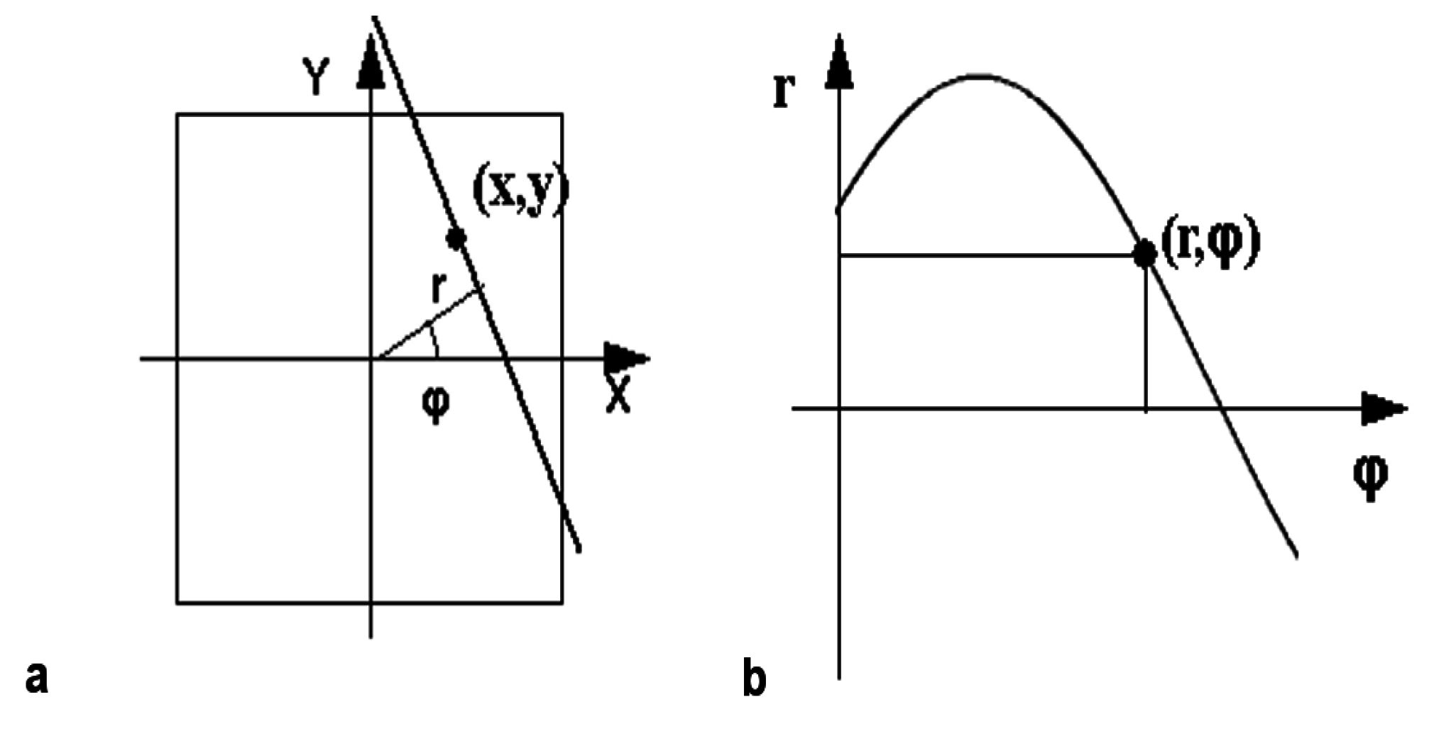
25]. The rule is based on the detection of objects from a given class by a voting procedure. This procedure is performed on parameter spaces that describe shapes; each point increases the counter (accumulator) value in the position corresponding to parameters it could be related to. After processing of all image points, the local maximum values in the parameter space describe the detected probable parameters of shapes. In practice, it is necessary to quantify the parameter values. In the simplest case of detection of straight lines, the line inclination angle φ (0 ≤
φ < π) and the distance from the origin of the co-ordinate system
r (the range depends on the image diagonal) could be used, as presented in
Figure 4.
Figure 4.
The image space (a) and the diagram (b) in the parameter space for an individual point.
Figure 4.
The image space (a) and the diagram (b) in the parameter space for an individual point.
For each point P(x,y), all cells of the accumulator that fit Equation (4) will be increased by a unit. It should be noted that, for each image point, it is necessary to determine the
r value for each
φ from the assumed range (
Figure 4).
The Hough transform can be generalized for other cases [
21,
25,
26]. Using the plane description by means of Equation (3), we can determine three parameters:
r,
φ and
ω. Based on the angles φ (−π/2 ≤ φ < −π/2) and ω (0 ≤ ω < π), we must determine the
r value for each point X, Y and Z from the TLS data (Equation (4)). The counters need to be similarly increased. In this case the parameter space is three-dimensional, which causes difficulties for graphical representation. For computer processing, this means utilization of a three-dimensional instead of a two-dimensional array. This obviously requires more memory and computation time (reflected in
Table 1).
Table 1.
Comparison of different plane detection methods.
Table 1.
Comparison of different plane detection methods.
| Algorithm | Sub-Sampling | Computation Time (s) | Main Wall Parameters | Number of Points in First Wall (% Total) |
|---|
| First Wall | Next | ω (°) | φ (°) | R (m) |
|---|
| RANSAC 3D | 1:20 | 395 | 50–100 | 101.6 | 0.57 | 3.65 | 37 |
| RANSAC 2D | 1:20 | 85 | 60 | 102.2 | - | 3.74 | 34 |
| Region growing | 1:20 | 1000 | - | 100.6 | 0.99 | 3.44 | 30 |
| Hough 2D | - | 15 | 10 | 102.0 | - | 3.70 | 33 |
| Hough 3D | - | 820 | 100 | 102.0 | 1.01 | 3.72 | 34 |
3.4. Automatic Generation of Intensity Orthoimages
The hierarchical and ordered structure of data recorded is an advantage of acquisition by terrestrial laser scanning (
Figure 2b). Such an approach, which is based on an assumed fixed scanning interval, explicitly defines the interpolation method that is applied for generation of the digital surface model (DSM) in the GRID form. Additionally, it allows us to recover the “missing points” (
i.e., those deleted in the data filtration process) based on the nearest points. This is why the
Triangular Irregular Network (TIN) interpolation method would be unsuitable.
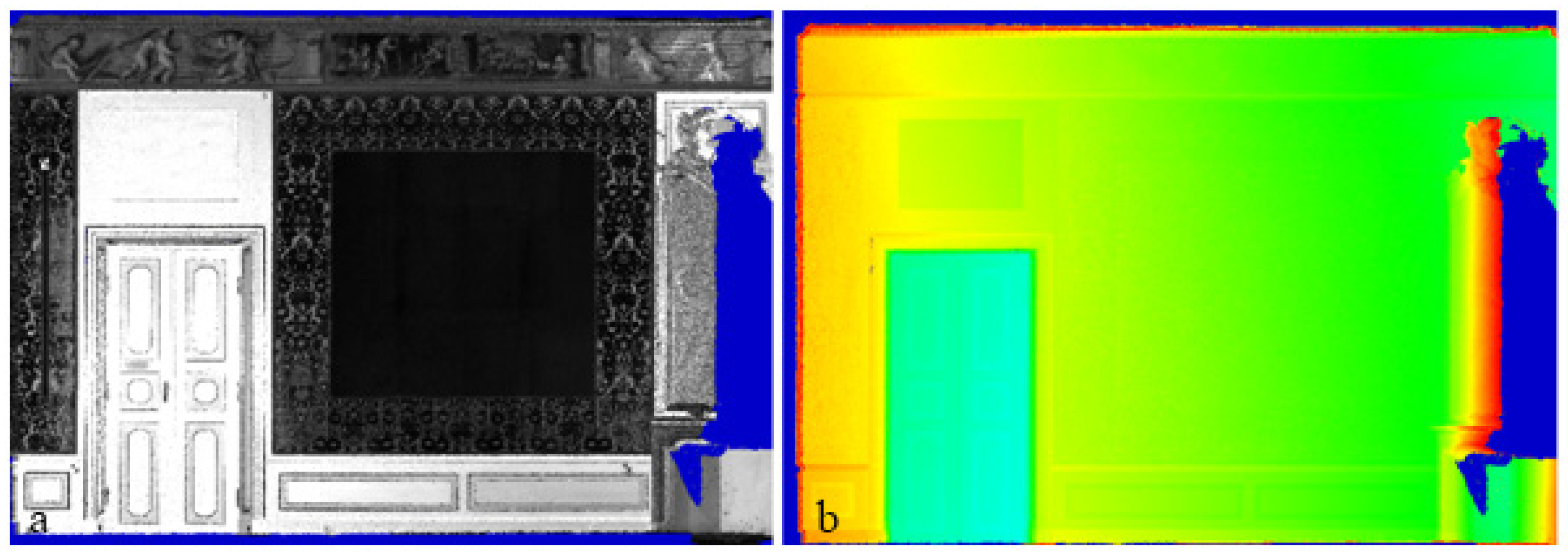
As a result, the orthoimages are obtained for use in further investigations into automation of the orientation of terrestrial digital images (
Figure 5a). Additionally, depth is recorded for each orthoimage, as well as the intensity of the laser beam reflection (
Figure 5b).
Figure 5.
(a) Intensity orthoimage—Ground Sample Distance (GSD) = 2 mm; (b) map of depth.
Figure 5.
(a) Intensity orthoimage—Ground Sample Distance (GSD) = 2 mm; (b) map of depth.
3.5. Detection of Keypoints—SIFT and SURF
3.5.1. SIFT (Scale Invariant Feature Transform)
The SIFT algorithm allows for the detection (extraction) of characteristic points (“keypoints”) in four main steps: scale-space extreme detection, keypoint localization, orientation assignment, and keypoint description. In the first step, the Gaussian difference function is used to detect potential characteristic points independently of the orientation scale. Areas located using the Difference of Gaussian (DoG) detector are described by the 128-dimensional vector, divided by the square root of the total squares of its elements, in order to achieve the invariance of changes in illumination [
27].
3.5.2. SURF (Speeded-Up Robust Features)
The SURF algorithm was developed in response to SIFT in order to allow reception of similar results within a shorter time. Like SIFT, it is independent of scale and rotation, due to the use of the Hessian matrix during computation. The use of an integrated image in the SURF algorithm allows simple approximation of the Hessian matrix determinant using a rectangular filter (not DoG as in the case of SIFT). This reduces the computational complexity [
28].
3.6. Orientation of Images in Relation to Intensity Orthoimages—SIFT
The objective of our experiments was to investigate the possibility of using “free-hand” terrestrial images for orthorectification or colouring of a point cloud. Although our scanners are equipped with built-in digital cameras that acquire images during scanning, these are characterized by low resolution and geometric quality [
29].
In generating high-resolution orthoimages of cultural heritage objects, it is important to achieve high geometric and radiometric quality. For this reason, it is important to acquire “free-handed” images from positions different to those of the scanner stations. In the methodology proposed by the authors, orientation of images in relation to the point cloud is performed automatically, using the SIFT algorithm for the detector and the descriptor, which searches for tie points.
Common problems that occur in the acquisition of images of complex architectural objects relate to the maintenance of the reproducibility of the focal length and the limited possibility of framing appropriate parts when using fixed-focal-length lenses. The original application, based on processed algorithms from the OpenCV library,was used for image orientation in relation to scans. For determination of an image’s exterior orientation elements, the perspective transformation algorithm was used, implemented in the OpenCV library [
13,
30].
The camera calibration matrix [
13,
30] contains information on changes of the camera focal length f
x, f
y, depending on the pixel dimension in the X and Y directions and the co-ordinates of the position of the camera’s principal point (c
x and c
y, respectively).
In order to determine the camera orientation parameters, the solvePnP function is used, which requires the following input parameters:
Output parameters were matrices, which included information about exterior orientation elements, i.e., the rotation matrix (rvec) and the translation vector (tvec).
The above approach requires knowledge of the camera calibration parameters (interior orientation). Another solution is possible, known as DLT (Direct Linear Transformation). Determined parameters include hidden parameters of interior and exterior orientation [
32,
33].
3.7. Terrestrial Images Orthorectification
A digital image is a faithful image of an object presented in the central projection [
13]. Unlike in an orthoimage, as the result of an orthogonal projection (
i.e., a map), distortion of a digital image results from height differences of the object and the inclination of the image. In the theoretical approach, an orthoimage is an image whose projection plane is parallel to the reference plane, and where all rays are perpendicular to those two planes.
For the needs of the cultural heritage inventory, true orthophoto images are created [
13,
34]. Transformation of information acquired in the central projection for the orthogonal projection relies upon the processing of every pixel of the source image into the orthoimage, using knowledge of exterior orientation elements and the digital surface model. An image pixel would then be mathematically assigned to the generated orthoimage pixel as a result of superposition. This projection may be forward or backward [
13]. In the case of forward projection, each subsequent pixel is processed and its corresponding pixel on the orthoimage.
In the case of backward projection, for each orthoimage pixel, the location of a corresponding pixels is found on the image.
4. Experiments
This section reports the experiments carried out on the influence of the quality and resolution of the point cloud on the quality of final products (
Figure 1).
4.1. Determination of a Plane
Several experiments were performed to find the best algorithm for plane determination.
4.1.1. The RANSAC Method
The first experiments were performed with the use of Point Cloud Library algorithms [
22]. The object pcl::SACSegmentation<pcl::PointXYZ> was selected from this library.After determination of appropriate data sources and parameters, plane coefficients were determined to meet the criteria. Additionally, the list of inliers was returned to allow a repeated search for successive planes with the use of unused points (outliers). Practical attempts to apply procedures for the complete source data, comprising 48 million points, proved that equipment resources did not allow sufficiently fast data processing. Only after 1:20 resampling were 16 regions obtained that corresponded to planes (see colours on
Figure 6); some points remained unclassified by any plane (presented in grey).
The maximum deviation from the plane was assumed to be 5 cm (computed deviations are presented in
Figure 6).This value was arbitrarily selected based on evaluation of the “depth” of the utilized point cloud (
Figure 3). Points located further than 5 cm from the theoretical plane therefore were not considered in the plane determination, since these are either gross errors or belong to other objects, such as the floor or the ceiling. Most of the pseudo-3D drawingwas performed using the open-source 3D point cloud and the mesh-processing software CloudCompare [
35].
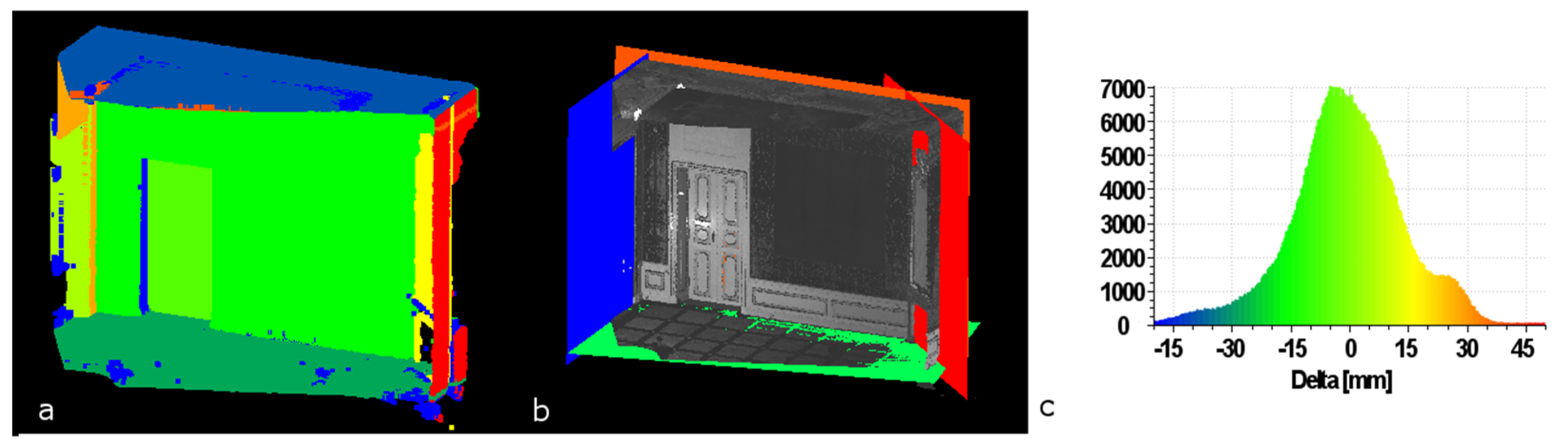
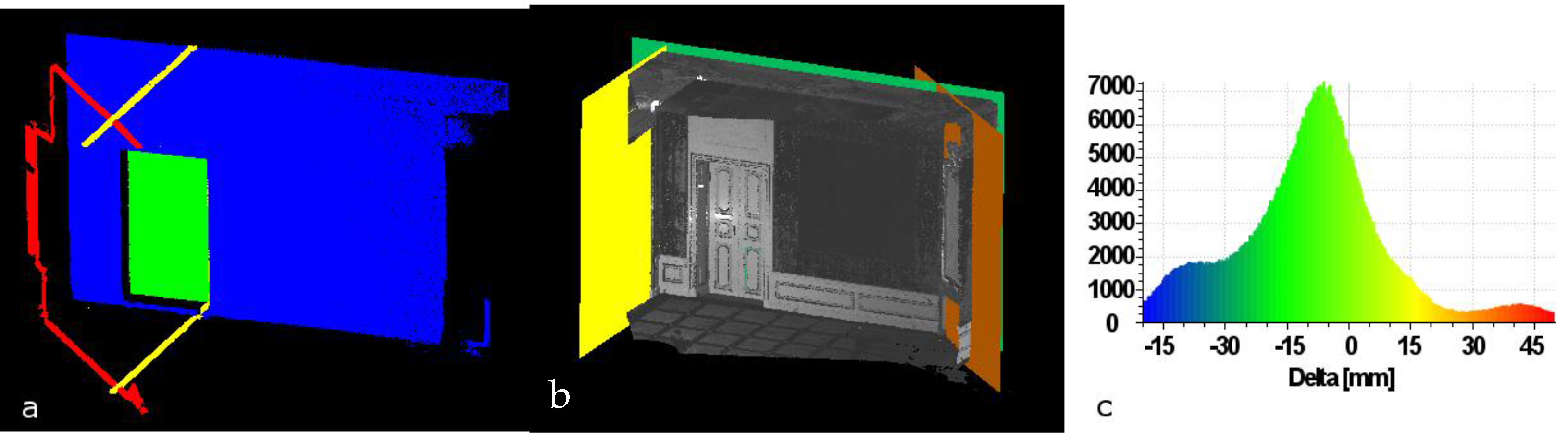
Figure 6.
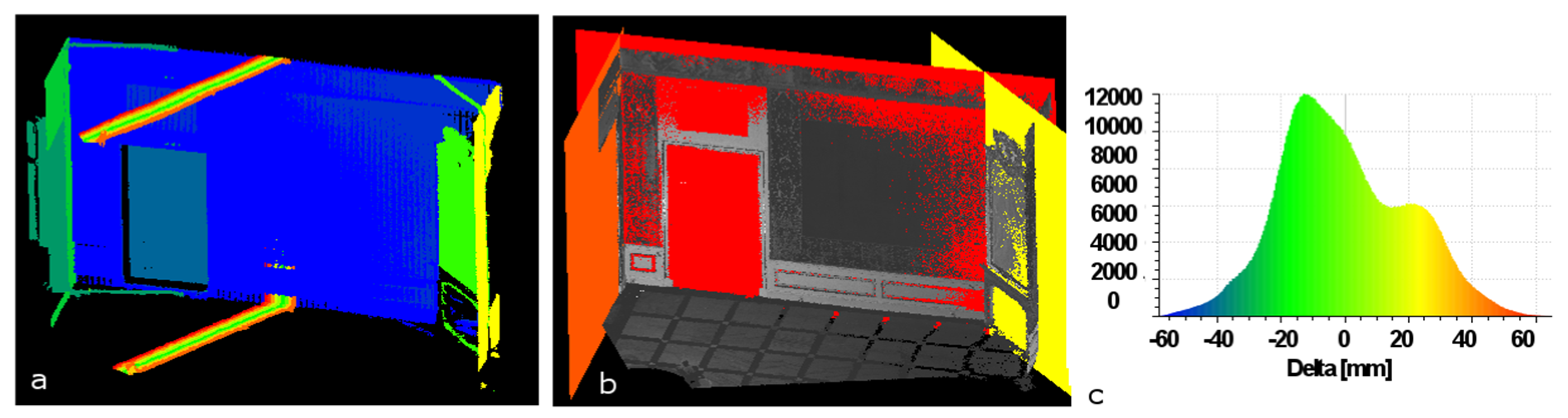
Planes detected by the PCL (RANSAC3D) algorithm: (a) Points on the same planes are marked with the same colour; (b) The rectangles describe the first four detected planes; (c) Histogram of the deviation.
Figure 6.
Planes detected by the PCL (RANSAC3D) algorithm: (a) Points on the same planes are marked with the same colour; (b) The rectangles describe the first four detected planes; (c) Histogram of the deviation.
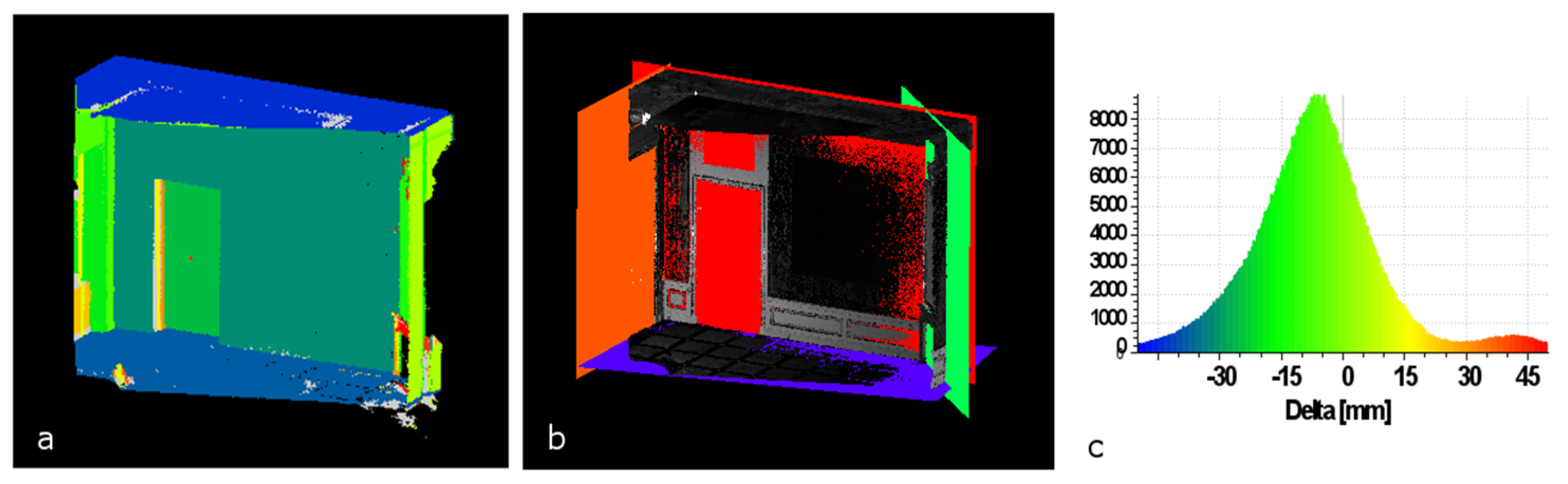
The presented figures permit us to observe that the algorithm tends to separate points into groups, although the
ω angle values are similar. The distribution of distance values from the theoretical wall surface is close to normal (
Figure 6); this allows us to conclude that the plane was correctly determined.
Similar procedures can be found in the “openMVG” (open Multiple View Geometry) library [
36,
37]. These include Max-Consensus, RANSAC, and AC-RANSAC (model and precision estimation), which also allow testing of the 2D version (neglecting the Z co-ordinate). Similarity was found between the size of the problem and the obtained results (
Figure 7).
Figure 7.
Planes detected by the 2D RANSACalgorithm: (a) Points on the same plane are marked with the same colour (the visible errors can be explained by inclusion of points on the floor and the ceiling); (b) The rectangles describe the first four detected planes; (c) Histogram of the deviation.
Figure 7.
Planes detected by the 2D RANSACalgorithm: (a) Points on the same plane are marked with the same colour (the visible errors can be explained by inclusion of points on the floor and the ceiling); (b) The rectangles describe the first four detected planes; (c) Histogram of the deviation.
4.1.2. Region Growing
The PCL library contains functions used for the determination of normal vectors for point clouds within the defined environment. The first attempts were made for the 2 mm neighbouring area, resulting in a high dispersion of normal vectors.
Due to the limitations of the equipment, it was necessary to perform 1:10 resampling and select the neighbourhood area as 10 mm in order to reduce the dispersion value.
Figure 8 and
Figure 9 present the components of the normal vector to neighbouring points in the cloud.
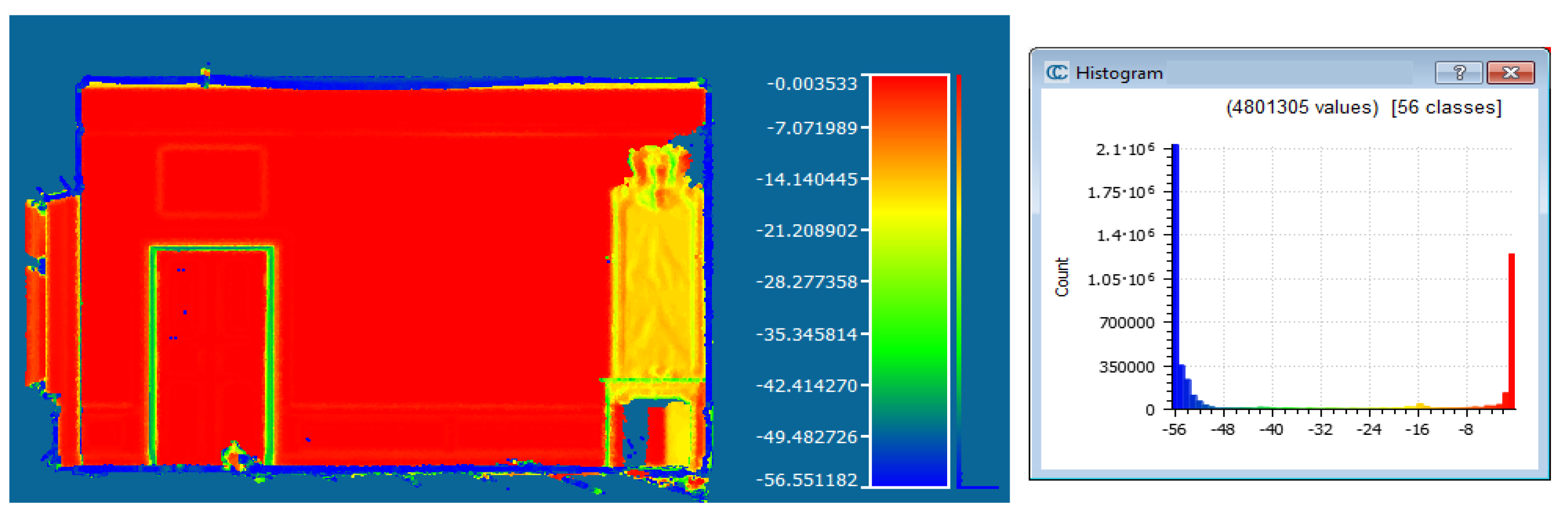
Figure 8.
Distribution of the deviation of the normal vector (Ny component), expressed in degrees, determined for the neighbourhood of 10 × 10 mm. Three maximum values are visible in the histogram; they correspond to the floor (in blue), the mirror above the fireplace (in yellow) and the wall (in red). It can be seen that the niche area of the door was not separated, although it is located at a different depth.
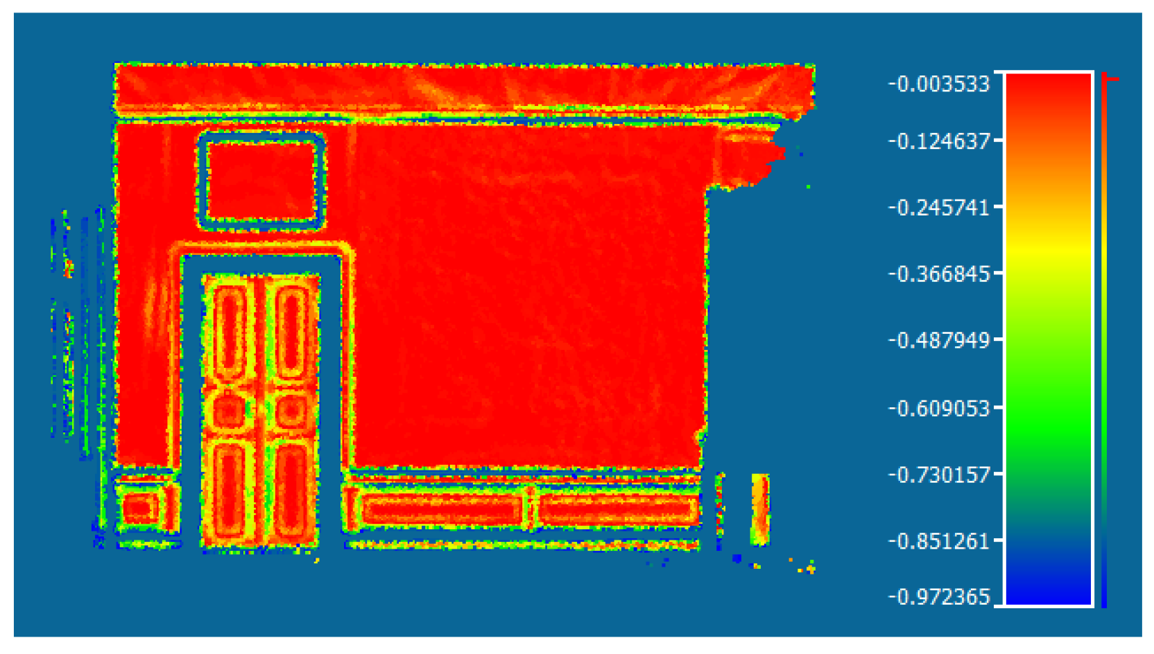
Figure 9.
Points for which the deviation of the Ny normal vector does not exceed 1 degree.
Figure 9.
Points for which the deviation of the Ny normal vector does not exceed 1 degree.
4.1.3. The 2D Hough Transform
The direct utilization of the Hough transform requires an image to be generated on a 2D plane,
i.e., that the XY co-ordinates be quantified and the Z co-ordinate neglected. The first experiments proved that, the use of simple procedures from the OpenCV library [
30,
31],does not obtain satisfactory results. The image is disturbed by points on the floor and the ceiling, and therefore there are no clear maximum values (
Figure 10b). Modification of this algorithm not by a unit, but by the number of cloud points that correspond to the given XY cell led to more promising results (
Figure 10c) than were obtained using the Canny algorithm, as presented in our previous paper [
18].
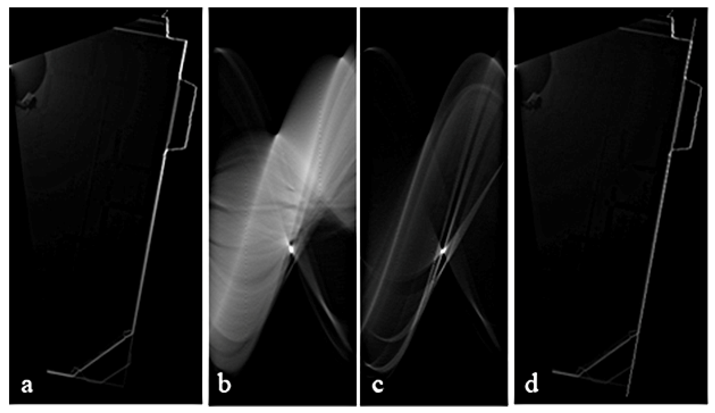
Figure 10.
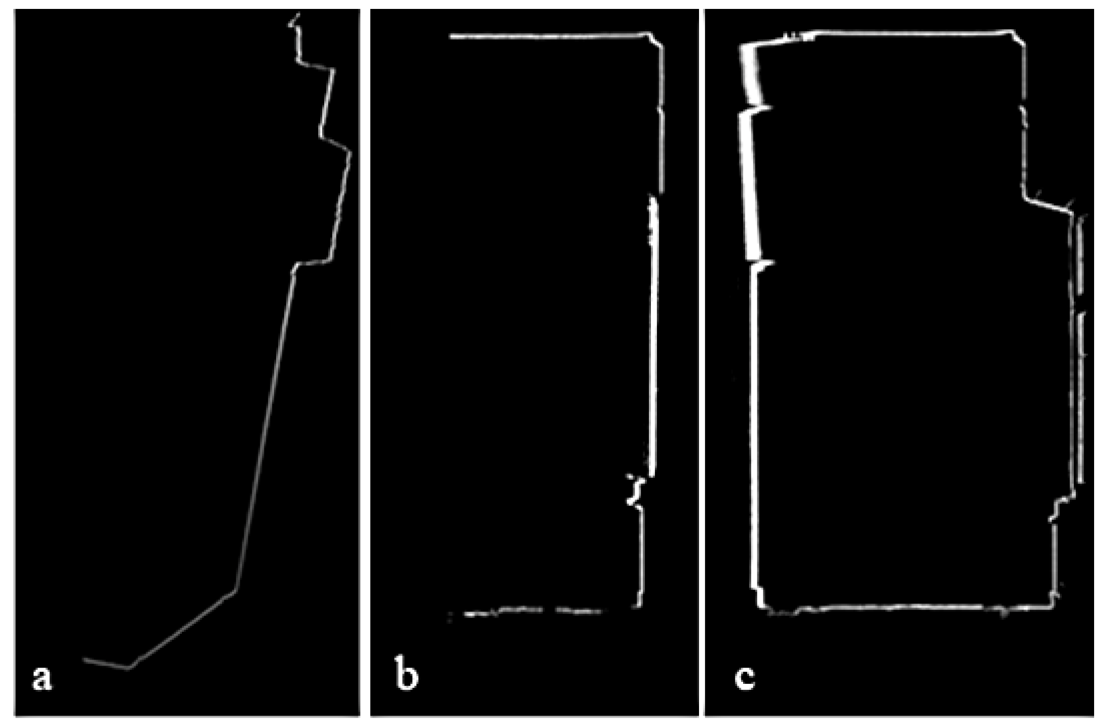
Example of 2D Hough transform: (a) The XY image—the brightness corresponds to the number of points included in the individual cell; the cell size has been assumed as 20 × 20 mm; (b) The parameter space when the counter is incremented by 1; (c) The parameter space when the counter is incremented by the number of points in a cell (the original algorithm)—the visible maximum corresponds to the direction of the wall; (d) The line corresponding to the maximum value from the image in (c), marked on the XY image.
Figure 10.
Example of 2D Hough transform: (a) The XY image—the brightness corresponds to the number of points included in the individual cell; the cell size has been assumed as 20 × 20 mm; (b) The parameter space when the counter is incremented by 1; (c) The parameter space when the counter is incremented by the number of points in a cell (the original algorithm)—the visible maximum corresponds to the direction of the wall; (d) The line corresponding to the maximum value from the image in (c), marked on the XY image.
Successive directions are determined after elimination of utilized points, zeroing of the counters, re-calculation of the parameter space, and selection of successive maximum values (
Figure 11).
Figure 11.
Planes detected by the 2D Hough transform: (a) Points on the same plane are marked with the same colour (the visible errors can be explained by inclusion of points on the floor and the ceiling); (b) The rectangles describe the first three detected planes; (c) Histogram of the deviation.
Figure 11.
Planes detected by the 2D Hough transform: (a) Points on the same plane are marked with the same colour (the visible errors can be explained by inclusion of points on the floor and the ceiling); (b) The rectangles describe the first three detected planes; (c) Histogram of the deviation.
In order to avoid quantification of XY co-ordinates, a new version of the software application was developed that determines the image in the parameter space, directly on the basis of real XY co-ordinates from the point cloud. However, since the image must be quantified in the parameter space, it turns out to be practically identical with the image presented in
Figure 11, albeit with considerably longer computing time—the value from Equation (4) must be determined for each of 48 million points, and in the previous version for 212 × 430 = 91,000 points only.
4.1.4. The 3D Hough Transform
Utilization of the 3D version requires the software developed by the authors. The quantified 3D image is created based on the XYZ point co-ordinates (the cell size is assumed as 2 × 2 × 2 cm).
Figure 12 illustrates the cross-sections.
Figure 12.
Example cross-sections of the 3D image utilized in the 3D Hough transform (the brightness corresponds to the number of points included in an individual cell): (a) XY image; (b) XZ image; (c) YZ image.
Figure 12.
Example cross-sections of the 3D image utilized in the 3D Hough transform (the brightness corresponds to the number of points included in an individual cell): (a) XY image; (b) XZ image; (c) YZ image.
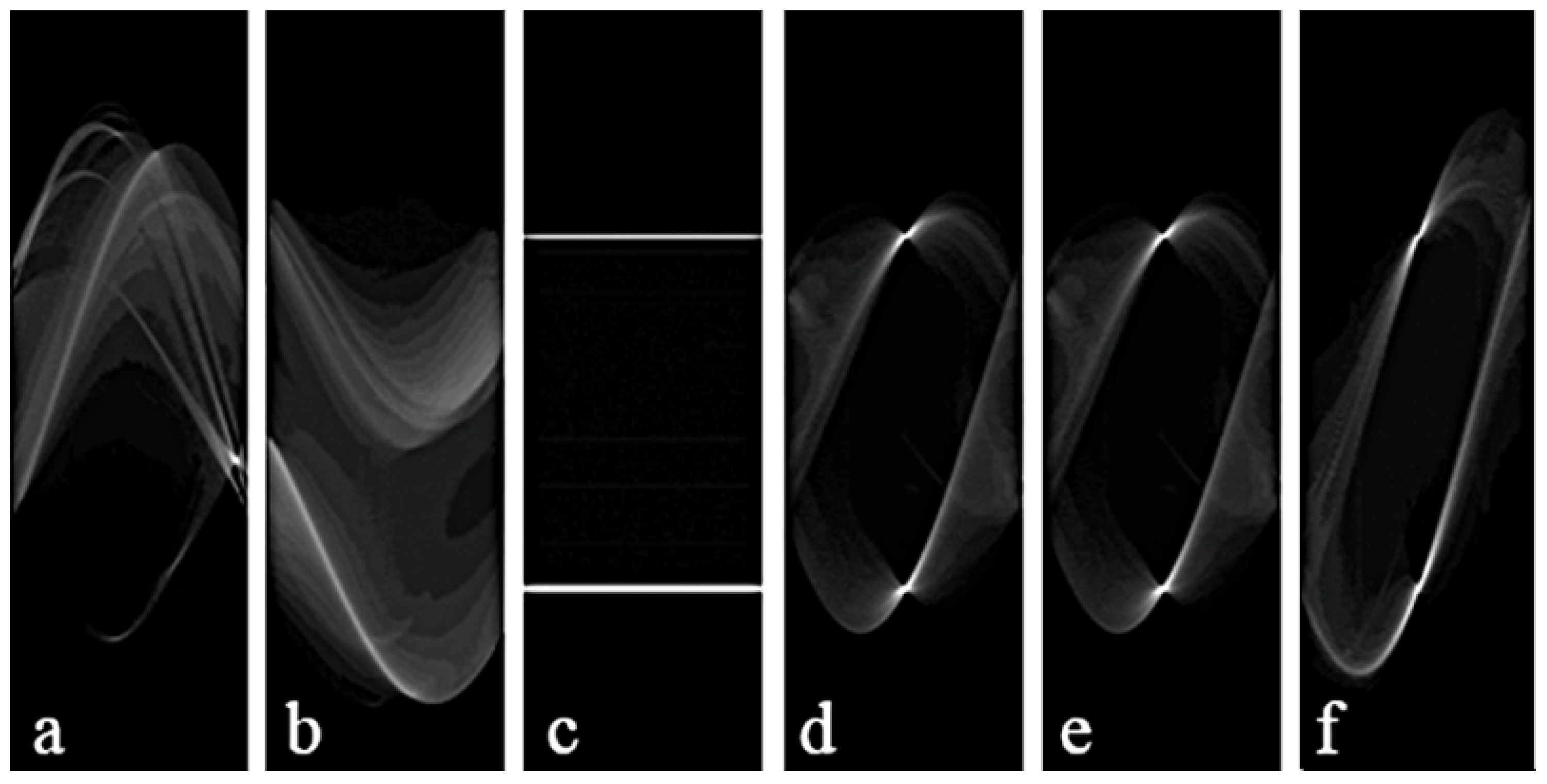
Then, the 3D image is generated in the parameter space by determining the r parameter as the ω, φ function and updating the counters by the number of points included in a corresponding XYZ cell. The angular resolution of 1 degree for
r = 2 cm is assumed. As mentioned above,the parameter space is three-dimensional and its presentation on a plane is difficult.
Figure 13 illustrates the parameter-space cross-sections.
Figure 13.
Example cross-sections of the domain of 3D parameters determined by the 3D Hough transform. The first three drawings show sections in the ω-r plane for the different parameters: φ: (a) φ = 0°; (b) φ = 45°; (c) φ = 90°. The next three show sections in the φ-r plane for the different parameters ω: (d) ω = 0°; (e) ω = 45°; (f) ω = 90°.
The search planes illustrated in
Figure 14 are almost identical to those used with the 3D RANSAC method because the calculated parameters are very similar (see
Table 1).
Figure 14.
Planes detected by the 3D Hough algorithm: (a) Points on the same plane are marked with the same colour; (b) The rectangles describe the first four detected planes; (c) Histogram of the deviation.
Figure 14.
Planes detected by the 3D Hough algorithm: (a) Points on the same plane are marked with the same colour; (b) The rectangles describe the first four detected planes; (c) Histogram of the deviation.
Similarly to the 2D case, the algorithm utilizing the original XYZ values instead of 3D images was also tested. The calculation time was unacceptable; therefore the results of this case have not been presented in this paper.
4.1.5. Results
It can be observed that all the algorithms tend to divide points into groups, though
ω values are similar (
Table 1). In practice, the distribution of distance values from the theoretical surface of the wall is always close to normal, which allows us to consider the determined parameters as correct.
Source data comprised 48 million points with an average density of 10 points per cubic cm. Calculations were performed using an i5 2.8 GHz, 8 GB RAM PC. The original software was used, with the exception of the case of 3D RANSAC.
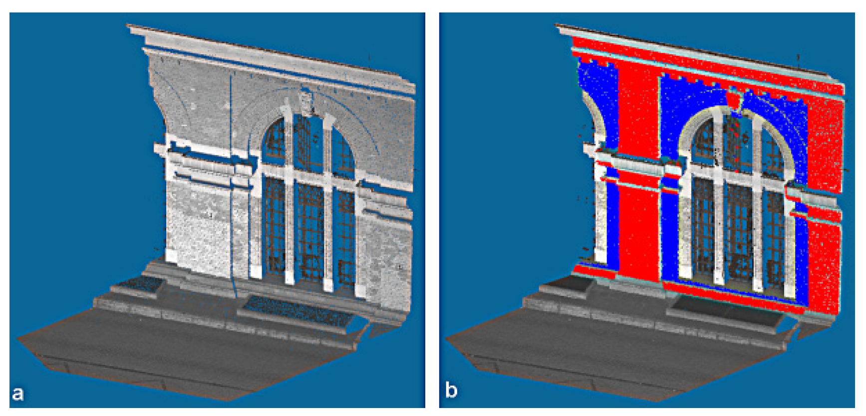
It can be seen that the computed plane normal vectors are similar. Significant differences in the values of R do not affect the further processing of orthoimages, as the projection is along the direction of R. The authors decided to use the 2D Hough algorithm because it gave the shortest computation time. Additionally, the 2D Hough algorithm not only detects planes but also allows similar planes to be connected that are not direct neighbours. Cultural heritage buildings have complicated structures and contain a lot of similar planes.
Figure 15 shows an example of planes detected by the 2D Hough algorithm.
Figure 15.
Results of 2D Hough algorithm for an object with many planes: (a) the raw point cloud; (b) detected points belonging to two different planes.
Figure 15.
Results of 2D Hough algorithm for an object with many planes: (a) the raw point cloud; (b) detected points belonging to two different planes.
4.2. Automatic Generation of Intensity Orthoimages
The orthoimage generation process was performed automatically using the LupoScan software. A point cloud of 2 mm resolution was used. Thus, it was not possible to generate an orthoimage with a Ground Sample Distance (GSD) smaller than 2 mm. The following input parameters were assumed:
NN interpolation;
assumed deviation of automatically generated plane = 5 cm;
buffer of projected points = ±3 × 5 cm;
resolution of generated object = 3 mm.
The resulting orthoimages (
Figure 5a) were then used for further investigations concerning automation of terrestrial images. Additionally, depth information was recorded for each orthoimage, as well as information concerning the laser-beam reflectance intensity (
Figure 5b).
4.3. Orientation of Images in Relation to Intensity Orthoimages—SIFT
Preliminary works were presented in [
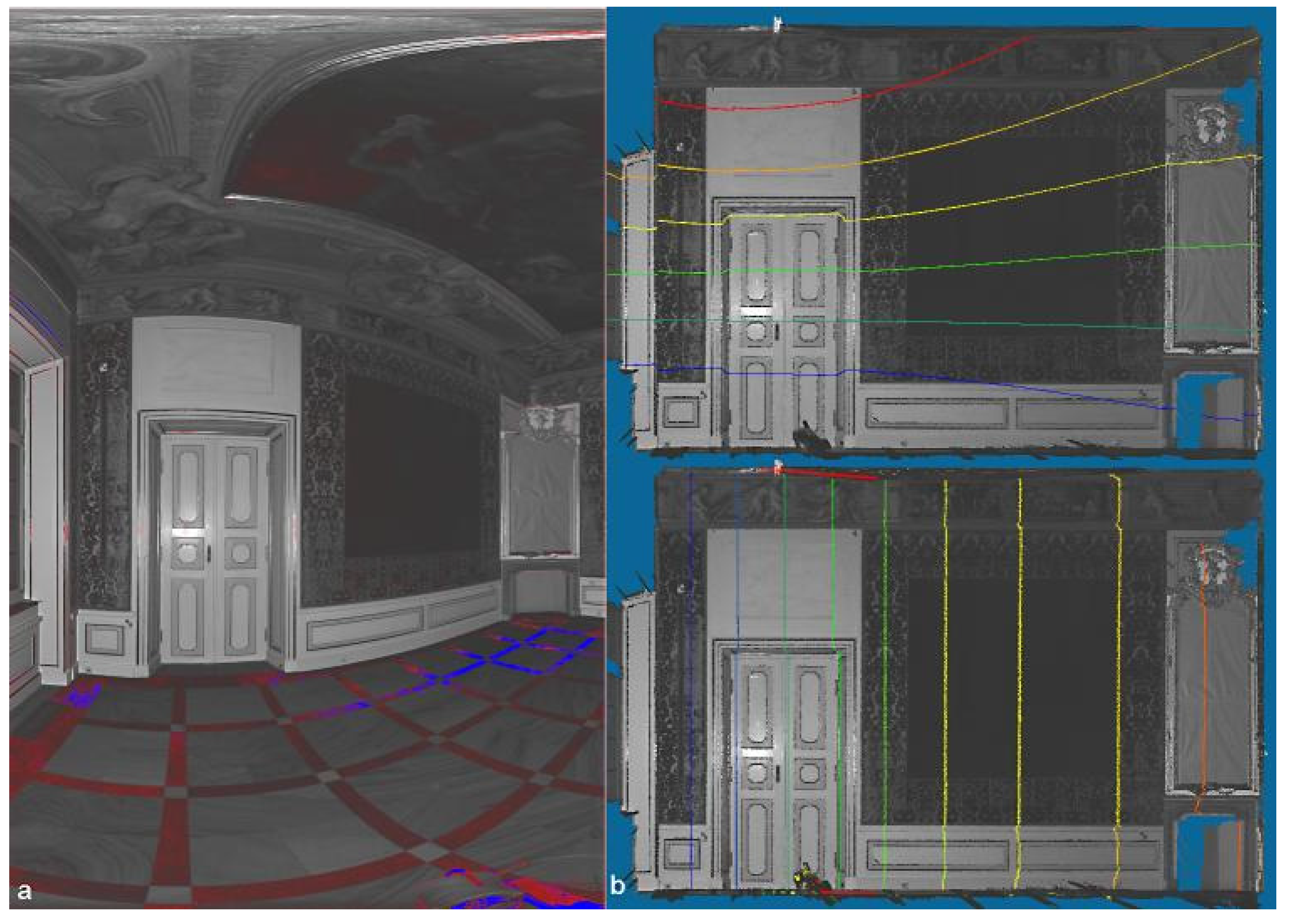
18]. This preliminary research was based on the utilization of two approaches to data orientation, with the use of cameras of determined interior orientation elements and images acquired with the use of a non-calibrated camera. The test site was the ruined castle in Iłża, which is characterized by relatively non-complicated surfaces whose shape could be considered as a plane. In the next stage, presented here, in order to test the methodology of the automatic generation of orthoimages some historical rooms at the Museum of King John III’s Palace in Wilanów were selected as test sites. These rooms are characterized by numerous decorative elements and sculptural details. The terrestrial image orientation process was carried out based on TLS data, according to the two different approaches:
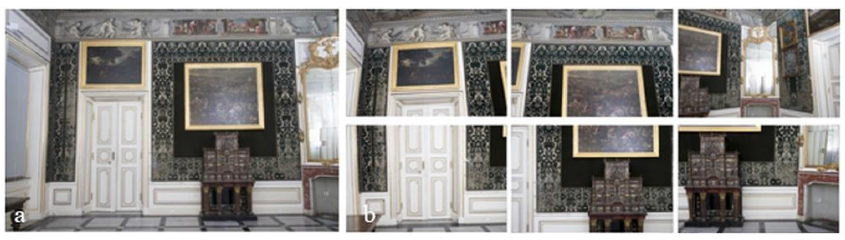
Variant I—the utilized image covered the entire area; the camera was calibrated in a test field; the exterior orientation elements were determined and considered further at the data processing stage (
Figure 16a).
Variant II—a group of images was acquired that covered the analysed area. The horizontal coverage of the images was 70% and the vertical coverage up to 50%. Self-calibration was performed and the interior parameters were considered in further data processing (
Figure 16b).
Figure 16.
Examples of used images: (a) Variant I: one image covering the entire orthoimage area; (b) Variant II: part of multiple images covering the entire orthoimage area.
Figure 16.
Examples of used images: (a) Variant I: one image covering the entire orthoimage area; (b) Variant II: part of multiple images covering the entire orthoimage area.
The images were processed in the following stages:
Use of this detector made it possible to detect evenly distributed keypoints, which were used as tie (homologous) points in the next step.
During the first step the gradient value and orientation for each keypoint was calculated. In order to compare and match the described features, the “Best match” function was used [
36].
Due to the different textures and constituent materials of cultural heritage objects, incorrect distribution of tie points may occur. An automatic procedure was developed for this eventuality, which may be applied for controlling the distribution of points before the adjustment is performed. At the first stage the algorithm divides images into four areas and checks whether the points are distributed approximately evenly. If one group of points is 10 times greater than another, an incorrect distribution is signalled. In the next step the algorithm checks whether the number of points in each image quarter is smaller than two (
i.e., eight points in the entire image). If such a situation occurs, the process is terminated and the image is not oriented. After this stage the adjustment using the least-square method is applied (Gauss-Markov).
The obtained results were controlled based on “checkpoints”.
4.3.1. Detection of Tie Points with the Use of the SIFT Algorithm (Authors’ Application)
The SIFT algorithm [
27] was applied to search for and match tie points, implemented in the OpenCV function library with default parameter values. Generated orthoimages were geo-referenced and the depth was recorded; this not only allowed the determination of field point co-ordinates in the orthoimage plane, but also the addition of the third dimension. These data allowed observations to be adjusted appropriately.
4.3.2. Orientation with the Use of Two Methods
Unfortunately, not all points that were automatically detected by the SIFT algorithm were correctly matched [
18]. The criterion for correct point qualification related to the difference between the co-ordinates of a point determined on an image and the calculated value. The process was performed automatically using the software developed by the authors. In order to set a filtering threshold a series of empirical tests were performed.
Variant I
Eight single images of four walls were used for testing and analysis. This approach allowed implementation of the orthorectification process without inclusion of a mosaic step. The advantage of using the images in this way was the possibility of eliminating the influence of texture repeatability on the number and quality of detected homologous points (
Figure 17).
The proposed algorithm allows to detect about 2254 tie points but unfortunately, about 11% of them was incorrect (
Appendix 1).
In order to enable an accurate analysis of image matching based on control points; deviations were also analysed. Due to the great number of tie points, the decision was made to present the results in the form of histograms showing deviations from the X and Y axes, respectively.
Figure 18 shows four example diagrams for one of the images.
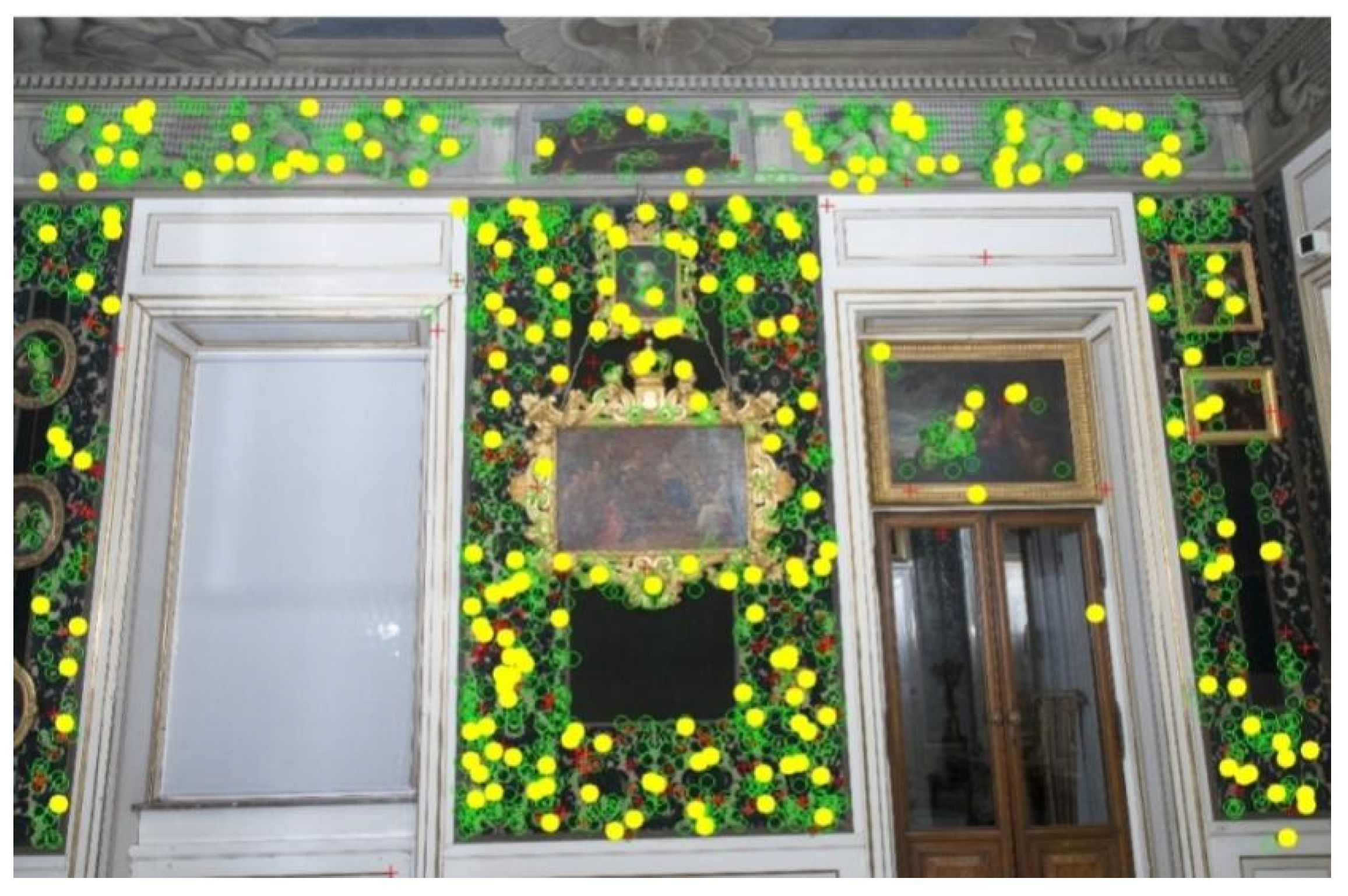
Figure 17.
Example of utilized image with control points in green and points eliminated from the adjustment process in red; a yellow “o”—a check point.
Figure 17.
Example of utilized image with control points in green and points eliminated from the adjustment process in red; a yellow “o”—a check point.
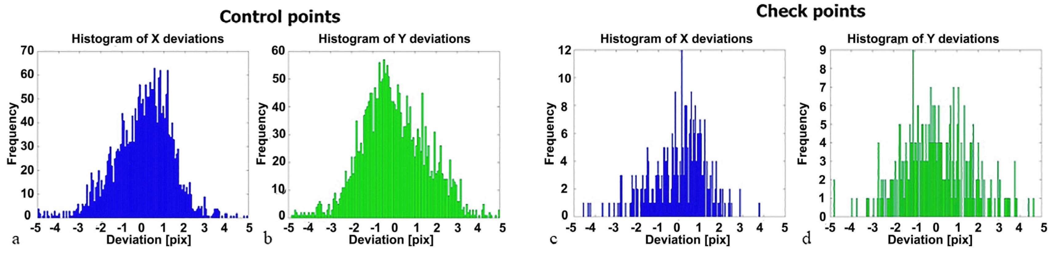
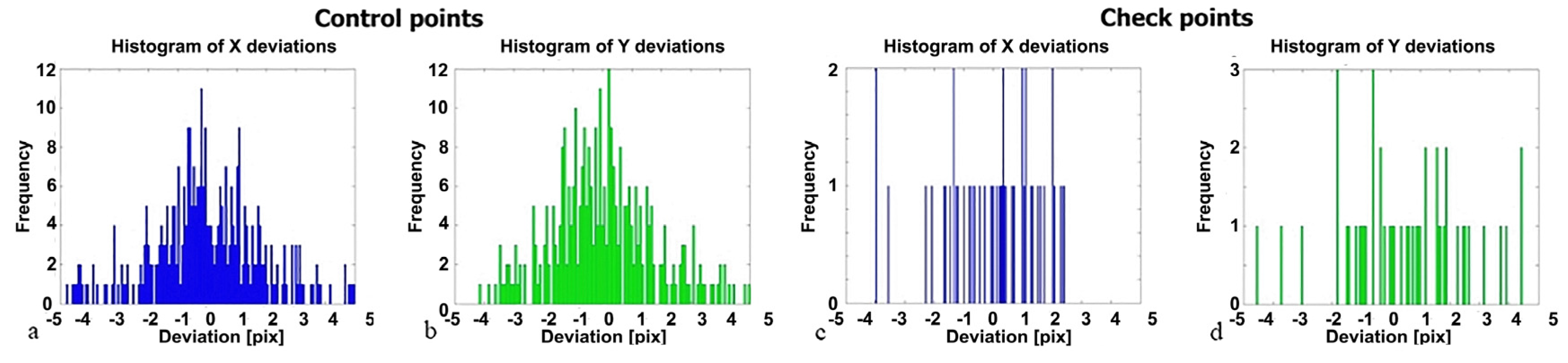
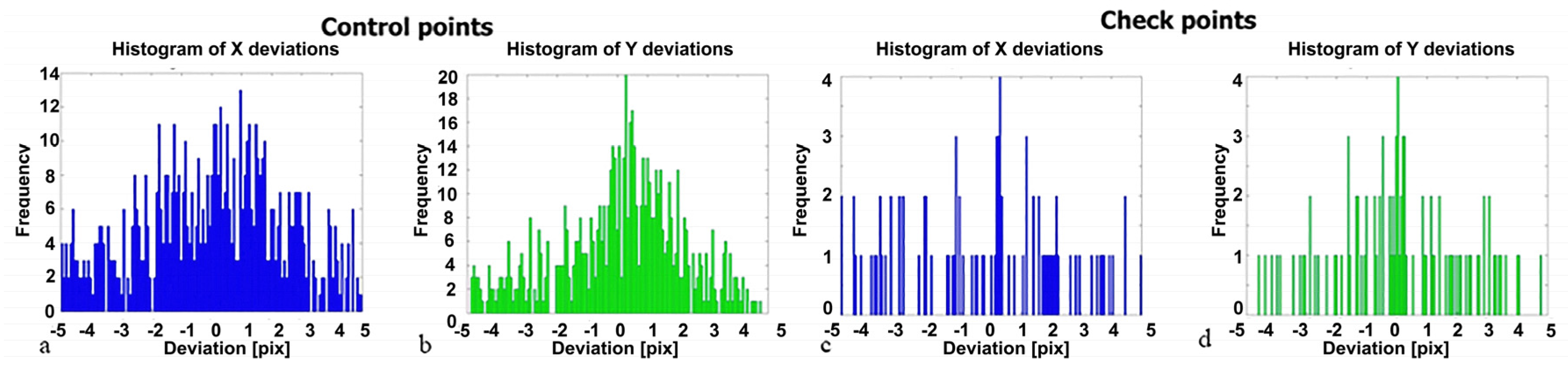
Figure 18.
Histograms of control-and check-point deviation: (a) X direction in pixels—control; (b) Y direction in pixels—control; (c) X direction in pixels—check; (d) Y direction in pixels—check.
Figure 18.
Histograms of control-and check-point deviation: (a) X direction in pixels—control; (b) Y direction in pixels—control; (c) X direction in pixels—check; (d) Y direction in pixels—check.
All analyses were performed using the authors’ original software, based on the Matlab package.
It is assumed in geodesy that least-square adjustment methods have Gaussian distribution [
13]. This confirms that only random errors occur, without gross errors. The possibility of evaluating the correctness of the results based on the normal distribution is influenced by the oscillation of the majority of deviations close to zero (the expected value). The control-point histograms show proximity to normal distribution, but are characterized by left- and right-hand obliquity (
Figure 18). The histograms are not shifted, which means that systematic errors do not exist. The obliquity may be considered as having been influenced by the terrestrial laser-scanner data. The distribution of the control points shows deviations in an interval of ±3 pixels, which corresponds to a range of ±3 mm.
The check-point histograms also show an approximately normal distribution, where the majority of deviations are oscillating around zero. This confirms the lack of systematic errors. The deviations are in an interval of ±3.5 pixels, which corresponds to a range of ±3.5 mm. This image orientation accuracy is sufficient for orthoimage generation of GSD 3 mm.
The applied intensity orthoimage (including the depth map) was characterized by a GSD of 3 mm, and the image had a GSD of 1 mm. The obtained mean standard deviation for matching of a digital image was equal to approximately three pixels, which is equal to the size of the intensity orthoimage.
Appendix 2 presents the extended statistical data.
Variant II
In the second variant, the group of images covering the entire wall was used for generation of the orthoimage.
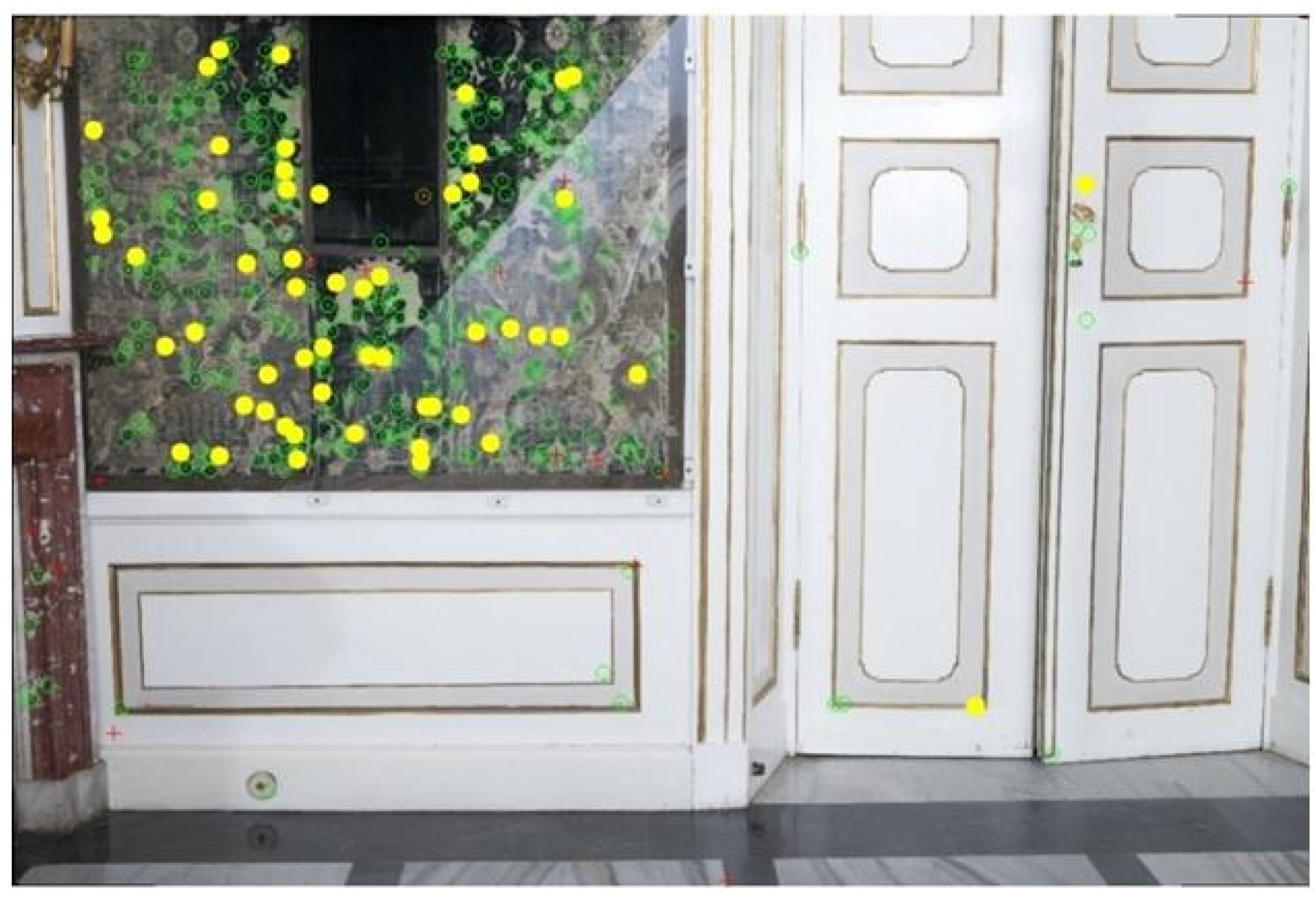
Due to the repetitive texture of the analysed object (decorated fabrics), the tie points were incorrectly detected by the algorithm. During the process of filtration about 67% of points were eliminated from further processing. Examples of images with tie points are presented in
Figure 19.
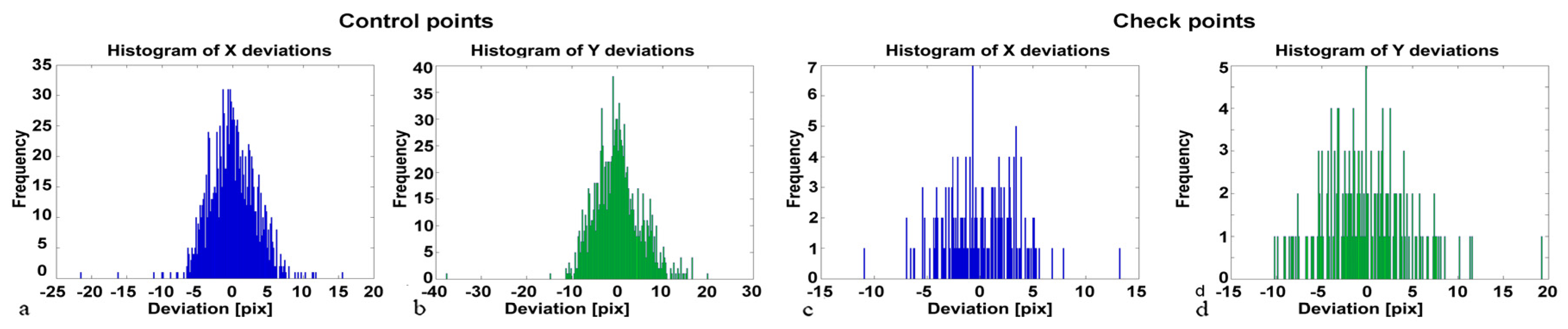
The analysed histograms show close-to-normal distribution, but are characterized by left- and right-hand obliquity (
Figure 20a,b). In the distribution of control points, deviations are in the interval of ±3.5 pixels, which corresponds to a range of ±3.5 mm. The check-points histogram (
Figure 20c,d) shows that Gaussian distribution was not achieved, due insufficient samples. Intervals of deviation values of between −2 and 2.5 pixels for the X coordinate and −2 and 5 pixels for the Y coordinate were taken to define accurate measurements; however, the majority of points oscillated between −2.5 and 2.5 pixels.
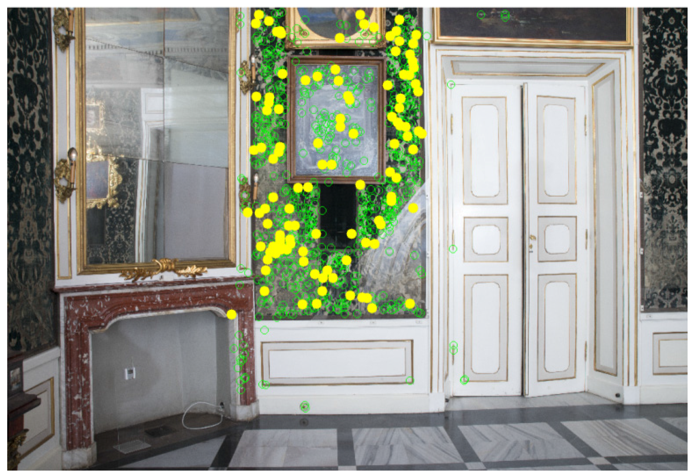
Figure 19.
Distribution of points detected in the single image (from a group) and in the orthoimage: green “o”—control points; red “+”—wrong matched points; yellow “o”—check points.
Figure 19.
Distribution of points detected in the single image (from a group) and in the orthoimage: green “o”—control points; red “+”—wrong matched points; yellow “o”—check points.
Figure 20.
Histograms of control- and check-point deviations: (a) X direction in pixels-control; (b) Y direction in pixels control; (c) X direction in pixels-check; (d) Y direction in pixels-check.
Figure 20.
Histograms of control- and check-point deviations: (a) X direction in pixels-control; (b) Y direction in pixels control; (c) X direction in pixels-check; (d) Y direction in pixels-check.
Due to an excessive number of points being eliminated during tie-point-detection control, the decision was made to superimpose masks on orthoimages in order to improve the quality and the number of points detected in the combination of images and orthoimages. The mask generation process was performed automatically. After initial orientation of an image covering a part of an orthoimage, the projections of image coordinates on the orthoimage plane were calculated. Generation of such a mask allows generation of a new orthoimage for re-orientation of images.
Utilization of masks for tie-point detection improved the number of correctly detected points. The proposed algorithm allows to detect 690 tie points however about 19% of them was incorrect (
Appendix 3).
Matching-point deviations were analysed and the results presented in the form of histograms.
Figure 21 presents examples of four diagrams.
Figure 21a,b shows that Gaussian distribution was not achieved. An interval between −2 and 2.5 pixels for the X coordinate and −2 and 5 pixels for the Y coordinate were taken as measures of accuracy; however, the majority of points oscillated between −5 and 5 pixels, corresponding to a range of ±5 mm. In the case of the check points (
Figure 21c,d), deviations are around ±5 pixels, corresponding to a range ±5 mm. Extended statistics are shown in
Appendix 4.
The obtained maximum values of standard deviations for matching of a digital image were equal to approximately four pixels, close to the size of the intensity orthoimage.
These analyses present only the accuracy of image orientation in relation to TLS data.
Figure 21.
Histograms of control- and check points deviations: (a) X direction in pixels-control; (b) Y direction in pixels-control; (c) X direction in pixels-check; (d) Y direction in pixels-check.
Figure 21.
Histograms of control- and check points deviations: (a) X direction in pixels-control; (b) Y direction in pixels-control; (c) X direction in pixels-check; (d) Y direction in pixels-check.
4.3.3. Orientation Using 3D DLT Method
Another method of orientation of images in relation to terrestrial laser-scanning data is the DLT (
Figure 22). In order to test the efficiency of this method, several images covering the investigated area were analysed to assess the quality of the generated orthoimage close to the area borders. When the DLT method is applied it is not possible to directly utilize interior orientation elements obtained from calibration in particular distortion. Image orientation using the DLT method takes 11 coefficients (or more when deformations are caused, for example, by distortion) into consideration. DLT is performed separately for each image; therefore, it is not possible to apply the camera calibration
a priori; it is performed separately for each image. It is also impossible to determine DLT coefficients if all matching points are located on one plane, which is highly probable in the analysed cases.
Figure 22.
Example of utilized image with points used for orientation (control points, in green) and yellow “o”—check points.
Figure 22.
Example of utilized image with points used for orientation (control points, in green) and yellow “o”—check points.
Control point deviations were also analysed, and the results presented as histograms showing deviations from the X and Y axes, respectively (
Figure 23).
Compared to the independent bundle method, the orientation results obtained with the DLT method are characterized by significantly lower orientation accuracy for control points. Obtained deviations for check points reach as high as 20 pixels (GSD 3 mm).
Figure 23.
Histograms of deviations of control and check points: (a) X direction in pixels-control; (b) Y direction in pixels-control; (c) X direction in pixels-check; (d) Y direction in pixels-check.
Figure 23.
Histograms of deviations of control and check points: (a) X direction in pixels-control; (b) Y direction in pixels-control; (c) X direction in pixels-check; (d) Y direction in pixels-check.
4.4. RGB Orthoimages Generation and Inspection (SURF Algorithm)
The process of generation of colour orthoimages was performed automatically using the LupoScan package. Due to the nature of the regular DSM, the backward projection based on interpolation of the radiometric values for all nodes of the network was applied. This avoided deformations of radiometric values and allowed colour to be maintained, as required in conservation analyses.
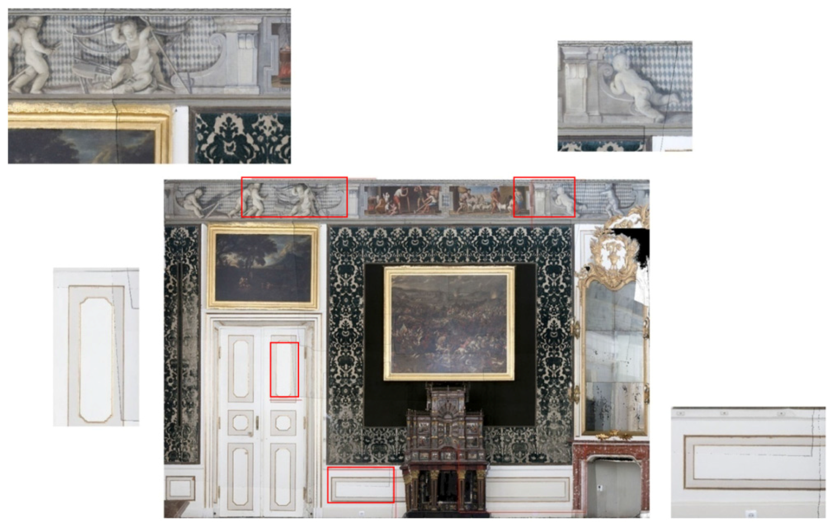
The final orthoimage (after mosaicking) is shown in
Figure 24 (
Appendix 5). The red rectangle shows the places where two different images overlap. It can be seen that there are no parallaxes, only differences in colour.
Figure 24.
RGB orthoimage with marked overlaps and seam lines.
Figure 24.
RGB orthoimage with marked overlaps and seam lines.
In order to analyse the accuracy of the generated RGB orthoimage, it was compared with the intensity orthoimage (
Table 2).
Table 2.
Deviation between check points on intensity orthoimages and RGB orthoimages (GSD—3 mm).
Table 2.
Deviation between check points on intensity orthoimages and RGB orthoimages (GSD—3 mm).
| Id | RMSE | >2 RMSE |
|---|
| | X (mm) | Y (mm) | X (%) | Y (%) |
|---|
| 1 | 2.69 | 3.12 | 2.5 | 1.8 |
| 2 | 2.03 | 2.00 | 2.4 | 2.4 |
| 3 | 2.15 | 2.06 | 4.0 | 4.6 |
| 4 | 2.19 | 1.76 | 10.6 | 13.4 |
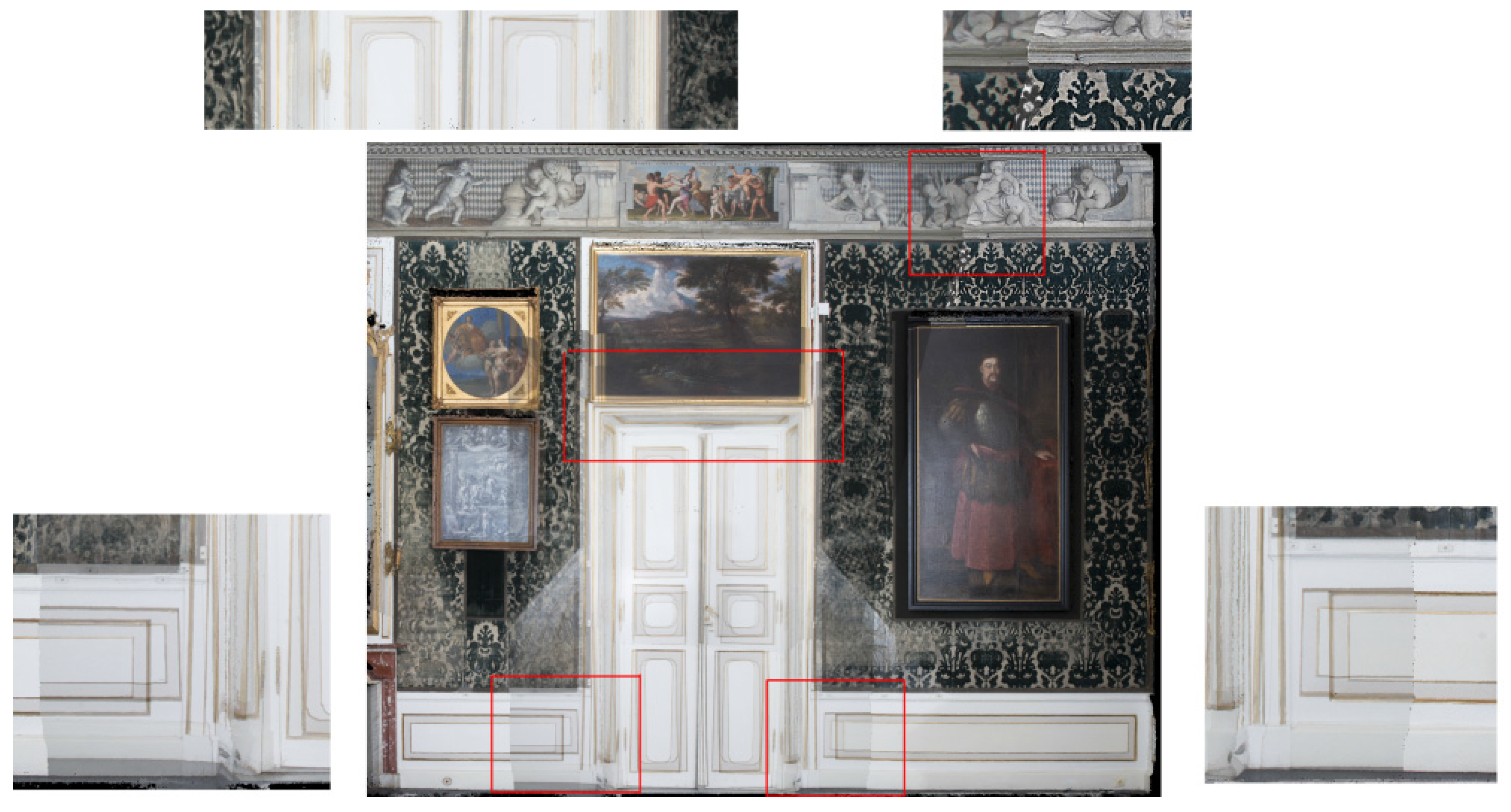
Figure 25 shows considerable displacements at the image borders. This results from uneven distribution of automatically detected matching points and from distortion, which has not been considered in the utilized 3D DLT method.
Figure 25.
An RGB image with displacements resulting from inaccurately oriented images using the 3D DLT method.
Figure 25.
An RGB image with displacements resulting from inaccurately oriented images using the 3D DLT method.
In order to analyse the accuracy of the generated RGB orthoimage, it was compared with the intensity orthoimage. The obtained root mean square error (RMSE) values were: X—5.91 mm, Y—6.76 mm, Z—6.76 mm. For 28% of points, the deviation was larger than 2 RMS.
5. Discussion
The experiments proved that, depending on the scanner and the surface type of the analysed object, the “depth” of the cloud of points is often great; indeed, it can be greater than the scan resolution (see
Section 3.1.). Therefore, the quality of the point cloud has an important influence on the correctness of the determined projection plane, the quality of the image generated in the intensity, and the accuracy of the orientation of terrestrial images. The present authors propose that every orthoimage generation process, particularly in relation to cultural heritage objects, should be preceded by an initial analysis of the geometric quality of the point cloud. In the experiments presented in this paper, original software applications were used.
Five methods of detection of the projection plane of an orthoimage in the point cloud were tested (described in
Section 4.1.). Each of the search methods produced similar results, but some turned out to be highly time consuming [
23,
24,
25,
30]. Based on the performed analyses, it can be stated that the fastest implementation of automatic detection of a plane is with the modified Hough 2D algorithm (
Table 1). In order to verify the operations of particular methods, the original software application was developed in C
++; this will be modified in further experiments.
Due to the fact that the orientation process of images requires searching for homologous points, CV algorithms—the detector and descriptor SIFT—were used for that purpose. The experiments were performed in two variants: in the first variant, an individual image covering the entire investigated area was used, and in the second variant a group of images covering the entire area (see
Section 4.3.2.). Matched points were divided into two groups—control and check points—for orientation and checking. For the first variant, a detailed accuracy analysis is presented in
Appendix 1; the maximum relative error is equal to 0.2%. For the second variant, the solution utilized the entire intensity orthoimage and the mask that limits the projected area. When the area is not limited by the mask, the points are incorrectly matched by the SIFT descriptor (about 67% incorrectly matched points) [
27]. Tests were performed towards the automation of the process of defining the mask on the intensity image. The basic version of the 3D DLT method used here involves no interior orientation elements obtained from calibration. The accuracy of image orientation is therefore lower in relation to TLS data than when the independent bundle method is used, and generated images are characterized by considerable displacements in the common overlap areas.
A detailed geometric inspection of obtained orthoimages was performed for both variants. For this purpose, an independent CV algorithm—SURF—was applied. The intensity orthoimage and the RGB orthoimage were compared (see
Section 4.4.). The mean value of deviations was smaller than 2 pixels (GSD 3 mm).
6. Conclusions
The performed experiments proved that the orthoimage generation process can be automated, starting with generation of the reference plane and ending with automatic RGB orthoimage generation.
The proposed original approach, based on the modified Hough transform, allows us to considerably improve the process of searching for planes on entire scans, without the necessity of dividing them. Thus, the split-up scan with automatically generated planes simultaneously determines the number of orthoimages and the maximum deviations from the plane, which define the range (in front of and behind the plane) of points required for orthoimage generation. This new approach accelerates the orthoimage generation process and eliminates scanning noises from close-range scanners.
Utilization of orthoimages in the form of raster data, complemented by the third dimension, allows the application of CV algorithms to search for homologous points and perform spatial orientation of free-hand images. Such an approach eliminates the necessity to measure the control points.
This approach is not limited to images acquired by cameras integrated with scanners, which are characterized by lower geometric and radiometric quality. The solution is particularly recommended for generation of photogrammetric documentation of high resolution, when resolution and accuracy in the order of individual millimetres are required.
In conclusion, this approach with original software allows more complete automation of the generation of the high-resolution orthoimages used in the documentation of cultural heritage objects.
Supplementary Files
Supplementary File 1Acknowledgments
The authors would like to thank the reviewers and copy editors, whose helpful comments led to a better paper overall and also the Museum of King John III’s Palace in Wilanów for cooperation.
Author Contributions
Dorota Zawieska came up with the concept for the paper and wrote the first draft. Piotr Podlasiak performed algorithms and applications of plane direction of point clouds. Jakub Stefan Markiewicz implemented the OpenCV SIFT and SURF algorithms and performed algorithms and applications of data orientation. All authors participated in the data analysis.
Conflicts of Interest
The authors declare no conflict of interest.
References
- Mavromati, D.; Petsa, E.; Karras, G. Theoretical and practical aspects of archaeological orthoimaging. Int. Arch. Photogram. Remote Sens. 2002, 34, 413–418. [Google Scholar]
- Guarnieri, A.; Remondino, F.; Vettore, A. Digital photogrammetry and TLS data fusion applied to Cultural Heritage 3D modeling. In Proceedings of the ISPRS Commission V Symposium Image Engineering and Vision Metrology, Dresden, Germany, 25–27 September 2006.
- Grussenmeyer, P.; Landes, T.; Voegtle, T.; Ringle, K. Comparison methods of terrestrial laser scanning, photogrammetry and tacheometry data for recording of cultural heritage buildings. Int. Arch. Photogram. Remote Sens. Spat. Inf. Sci. 2008, 37, 213–218. [Google Scholar]
- Armesto-González, J.; Riveiro-Rodríguez, B.; González-Aguilera, D.; Rivas-Brea, M.T. Terrestrial laser scanning intensity data applied to damage detection for historical buildings. J. Archaeol. Sci. 2010, 37, 3037–3047. [Google Scholar]
- Giuliano, M.G. Cultural heritage: An example of graphical documentation with automated photogrammetric systems. Int. Arch. Photogram. Remote Sens. Spat. Inf. Sci. 2014. [Google Scholar] [CrossRef]
- Kersten, T.; Mechelke, K.; Maziull, L. 3D model of al zubarah fortress in Qatar—Terrestrial laser scanning vs. dense image matching. In Proceeding of the International Archives of the Photogrammetry, Remote Sensing Spatial Information Science, 2015 3D Virtual Reconstruction and Visualization of Complex Architectures, Avila, Spain, 25–27 February 2015.
- Ippoliti, E.; Meschini, A.; Sicuranza, F. Structure from motion systems for architectural heritage. A survey of the internal loggia courtyard of Palazzo Dei Capitani, Ascoli Piceno, Italy. In Proceeding of the International Archives of the Photogrammetry, Remote Sensing Spatial Information Science, 2015 3D Virtual Reconstruction and Visualization of Complex Architectures, Avila, Spain, 25–27 February 2015.
- Ballabeni, A.; Apollonio, F.I.; Gaiani, M.; Remondino, F. Advances in image pre-processing to improve automated 3D reconstruction. In Proceeding of the International Archives of the Photogrammetry, Remote Sensing Spatial Information Science, 2015 3D Virtual Reconstruction and Visualization of Complex Architectures, Avila, Spain, 25–27 February 2015.
- Alsadik, B.; Gerke, M.; Vosselman, G.; Daham, A.; Jasim, L. Minimal camera networks for 3D image based modeling of cultural heritage objects. Sensors 2014, 14, 5785–5804. [Google Scholar] [CrossRef] [PubMed]
- Chiabrando, F.; Donadio, E.; Rinaudo, F. SfM for orthophoto generation: A winning approach for cultural heritage knowledge. Int. Arch. Photogram. Remote Sens. Spat. Inf. Sci. 2015, 1, 91–98. [Google Scholar] [CrossRef]
- Markiewicz, J.S.; Zawieska, D. Terrestrial scanning or digital images in inventory of monumental objects? Case study. Int. Arch. Photogram. Remote Sens. Spat. Inf. Sci. 2014, 5, 395–400. [Google Scholar] [CrossRef]
- Ramos, M.M.; Remondino, F. Data fusion in cultural heritage—A review. In Proceeding of the 25th International CIPA Symposium on The International Archives of the Photogrammetry, Remote Sensing and Spatial Information Sciences, Taipei, Taiwan, 31 August—4 September 2015; pp. 359–363.
- Luhmann, T.; Robson, S.; Kyle, S.; Boehm, J. Close Range Photogrammetry and 3D Imaging, 2nd ed.; Walter De Gruyter: Boston, MA, USA, 2013. [Google Scholar]
- González-Aguilera, D.; Rodríguez-Gonzálvez, P.; Gómez-Lahoz, J. An automatic procedure for co-registration of terrestrial laser scanners and digital cameras. ISPRS J. Photogram. Remote Sens. 2009, 64, 308–316. [Google Scholar] [CrossRef]
- Remondino, F. Heritage recording and 3D modeling with photogrammetry and 3D scanning. Remote Sens. 2011, 3, 1104–1138. [Google Scholar] [CrossRef] [Green Version]
- Georgopoulos, A.; Tsakiri, M.; Ioannidis, C.; Kakli, A. Large scale orthophotography using DTM from terrestrial laser scanning. In Proceeding of the International Archives of the Photogrammetry, Remote Sensing Spatial Information Science, Istanbul, Turkey, 12–23 July 2004; Volume 35, pp. 467–472.
- Georgopoulos, A.; Makris, G.N.; Dermentzopoulos, A. An alternative method for large scale orthophoto production. In Proceedings of the CIPA 2005 XX International Symposium, Torino, Italy, 26 September–1 October 2005.
- Markiewicz, J.S.; Podlasiak, P.; Zawieska, D. Attempts to automate the process of generation of orthoimages of objects of cultural heritage. Int. Arch. Photogram. Remote Sens. Spat. Inf. Sci. 2015. [Google Scholar] [CrossRef]
- Moussa, W.; Abdel-Wahab, M.; Fritsch, D. An automatic procedure for combining digital images and laser scanner data. Int. Arch. Photogram. Remote Sens. Spat. Inf. Sci. 2012, 39, 229–234. [Google Scholar] [CrossRef]
- Meierhold, N.; Spehr, M.; Schilling, A.; Gumhold, S.; Maas, H.G. Automatic feature matching between digital images and 2D representations of a 3D laser scanner point cloud. In Proceedings of the ISPRS Commission V Mid-Term Symposium on Close Range Image Measurement Techniques, Newcastle upon Tyne, UK, 21–24 June 2010.
- Fischler, M.A.; Bolles, R.C. Random sample consensus: A paradigm for model fitting with applications to image analysis and automated cartography. Comm. ACM 1981, 24, 381–395. [Google Scholar] [CrossRef]
- PCL. Available online: http://pointclouds.org/ (accessed on 25 May 2015).
- Hough, P.V.C. Method and Means for Recognizing Complex Patterns. U.S. Patent 3,069,654, 18 December 1962. [Google Scholar]
- Duda, R.O.; Hart, P.E. Use of the Hough transformation to detect lines and curves in pictures. Commun. ACM 1972, 15, 11–15. [Google Scholar] [CrossRef]
- Ballard, D.H. Generalizing the Hough transform to detect arbitrary shapes. Pattern Recognit. 1981, 13, 111–122. [Google Scholar] [CrossRef]
- Overby, J.; Bodum, L.; Kjems, E.; Ilsoe, P.M. Automatic 3D building reconstruction from airborne laser scanning and cadastral data using Hough transform. Int. Arch. Photogram. Remote Sens. Spat. Inf. Sci. 2004, 35, 296–301. [Google Scholar]
- Lowe, D. Distinctive image features from scale-invariant key points. Int. J. Comput. Vis. 2004, 60, 91–110. [Google Scholar] [CrossRef]
- Bay, H.; Tuytelaars, T.; van Gool, L. SURF: Speeded Up Robust Features. Available online: www.vision.ee.ethz.ch/~surf/eccv06.pdf (accessed on 1 September 2015).
- Markiewicz, J.S.; Zawieska, D.; Kowalczyk, M.; Zapłata, R. Utilisation of laser scanning for inventory of an architectural object using the example of ruins of the Krakow Bishops’ Castle in Ilza, Poland. In Proceeding of the 14th GeoConference on Informatics Geoinformatics and Remote Sensing, Ilza, Poland, 19–25 June 2014; pp. 391–396.
- Bradski, G.; Kaehler, A. Learning OpenCV Computer Vision with the OpenCV Library; O’Reilly Media: Sebastopol, CA, USA, 2008. [Google Scholar]
- OpenCV. Available online: http://opencv.org/ (accessed on 12 May 2015).
- 3D Reconstruction Using the Direct Linear Transform with a Gabor Wavelet Based Correspondence Measure. Available online: http://bardsley.org.uk/wp-content/uploads/2007/02/3d-reconstruction-using-the-direct-linear-transform.pdf (accessed on 23 October 2015).
- Direct Linear Transformation(DLT). Available online: https://me363.byu.edu/sites/me363.byu.edu/files/userfiles/5/DLTNotes.pdf (accessed on 23 October 2015).
- Stavropoulou, G.; Tzovla, G.; Georgopoulos, A. Can 3D point clouds replace GCPs. ISPRS Ann. Photogram. Remote Sens. Spat. Inf. Sci. 2014, 5, 347–354. [Google Scholar] [CrossRef]
- Cloud Compare. Available online: http://www.danielgm.net/cc/ (accessed on 14 May 2015).
- OpenMVG. Available online: http://imagine.enpc.fr/~moulonp/openMVG/index.html (accessed on 30 May 2015).
- OpenMVG. Available online: https://openmvg.readthedocs.org/en/latest/ (accessed on 30 May 2015).
© 2015 by the authors; licensee MDPI, Basel, Switzerland. This article is an open access article distributed under the terms and conditions of the Creative Commons by Attribution (CC-BY) license (http://creativecommons.org/licenses/by/4.0/).


