
Improving Estimation of Evapotranspiration under Water-Limited Conditions Based on SEBS and MODIS Data in Arid Regions


Abstract
:
1. Introduction
2. Data
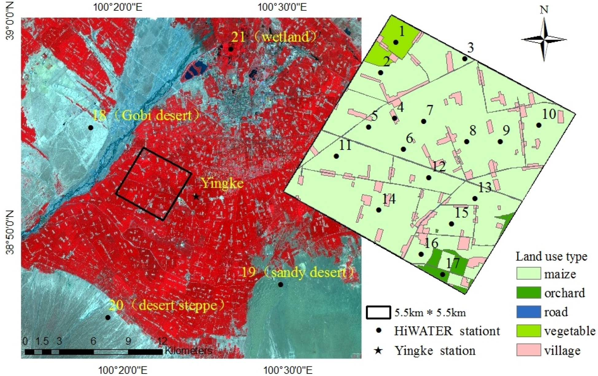
2.1. Study Area
2.2. Field Measurements


| Station | Longitude (E) | Latitude (N) | Elevation (m) | Land Cover | Observation Period |
|---|---|---|---|---|---|
| Yingke | 100.41033 | 38.85714 | 1519 | maize | 2007/11/5—2011/12/1 |
| S1 | 100.35813 | 38.89322 | 1552 | vegetable | 2012/6/10—2012/9/17 |
| S2 | 100.35406 | 38.88695 | 1559 | maize | 2012/5/3—2012/9/21 |
| S3 | 100.37634 | 38.89053 | 1543 | maize | 2012/6/3 —2012/9/18 |
| S4 | 100.35753 | 38.87752 | 1561 | village | 2012/5/10—2012/9/17 |
| S5 | 100.35068 | 38.87574 | 1567 | maize | 2012/6/4—2012/9/18 |
| S6 | 100.35970 | 38.87116 | 1562 | maize | 2012/5/9—2012/9/21 |
| S7 | 100.36521 | 38.87676 | 1556 | maize | 2012/5/28—2012/9/18 |
| S8 | 100.37649 | 38.87254 | 1550 | maize | 2012/5/14—2012/9/21 |
| S9 | 100.38546 | 38.87239 | 1543 | maize | 2012/6/4—2012/9/17 |
| S10 | 100.39572 | 38.87567 | 1534 | maize | 2012/6/1—2012/9/17 |
| S11 | 100.34197 | 38.86991 | 1575 | maize | 2012/6/2—2012/9/18 |
| S12 | 100.36631 | 38.86515 | 1559 | maize | 2012/5/10—2012/9/21 |
| S13 | 100.37852 | 38.86074 | 1550 | maize | 2012/5/6—2012/9/20 |
| S14 | 100.35310 | 38.85867 | 1570 | maize | 2012/5/6—2012/9/21 |
| S15 | 100.37223 | 38.85551 | 1556 | maize | 2012/5/10—2012/9/26 |
| S16 | 100.36411 | 38.84931 | 1564 | maize | 2012/6/1—2012/9/17 |
| S17 | 100.36972 | 38.84510 | 1559 | orchard | 2012/5/12—2012/9/17 |
| S18 | 100.30420 | 38.91496 | 1562 | Gobi desert | 2012/5/13—2012/9/21 |
| S19 | 100.49330 | 38.78917 | 1594 | sandy desert | 2012/6/1—2012/9/21 |
| S20 | 100.31860 | 38.76519 | 1731 | desert steppe | 2012/6/2—2012/9/21 |
| S21 | 100.44640 | 38.97514 | 1460 | wetland | 2012/6/25—2012/9/21 |
2.3. MODIS Land Data Products
2.4. Normalized Difference Water Index
3. Method
3.1. Surface Energy Balance System (SEBS)
3.1.1. Surface Energy Balance Terms
3.1.2. Calculation of Sensible Heat Flux
3.1.3. Calculation of Roughness Length for Heat Transfer
3.1.4. Calculation of Daily ET
3.1.5. Parameterization of Land Surface Parameters
3.2. Parameterization Scheme
4. Results
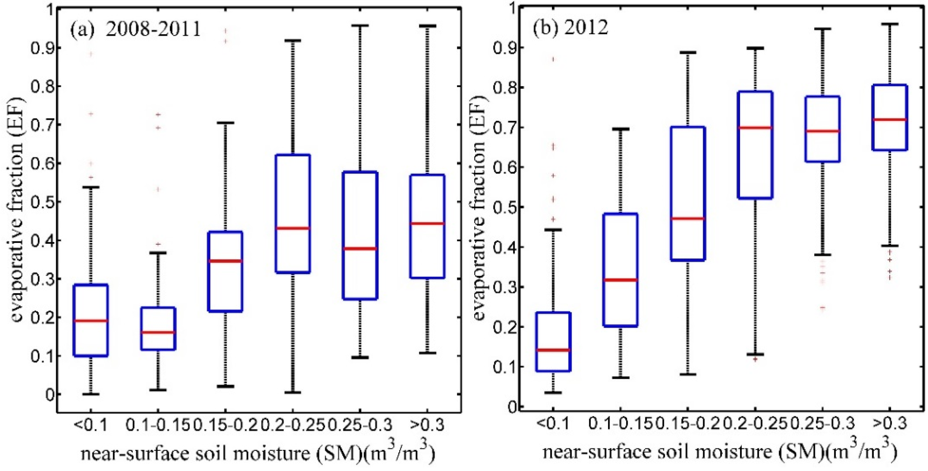
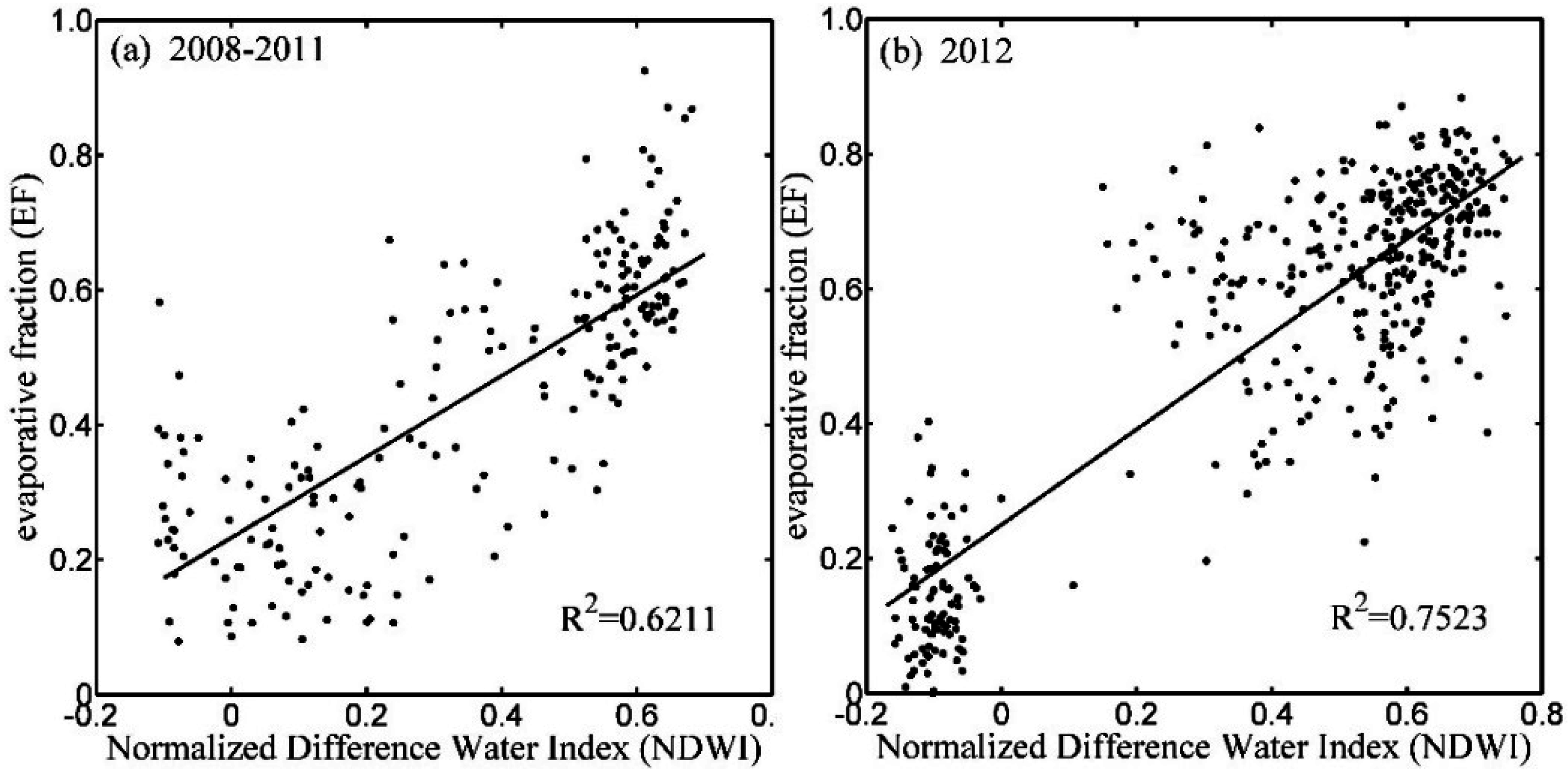
4.1. Influence of Soil Moisture on Evaporative Fraction


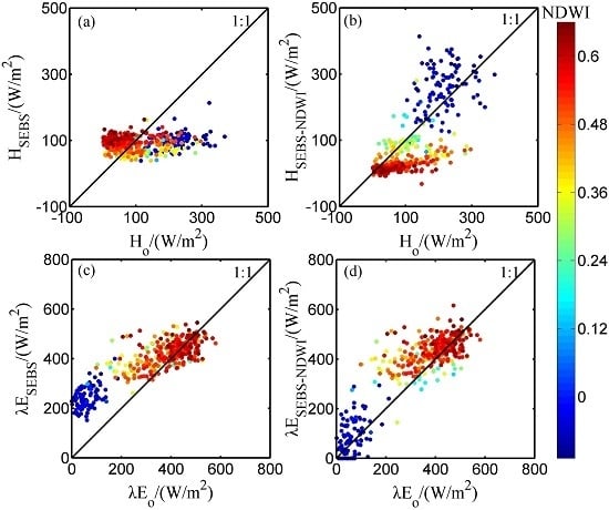
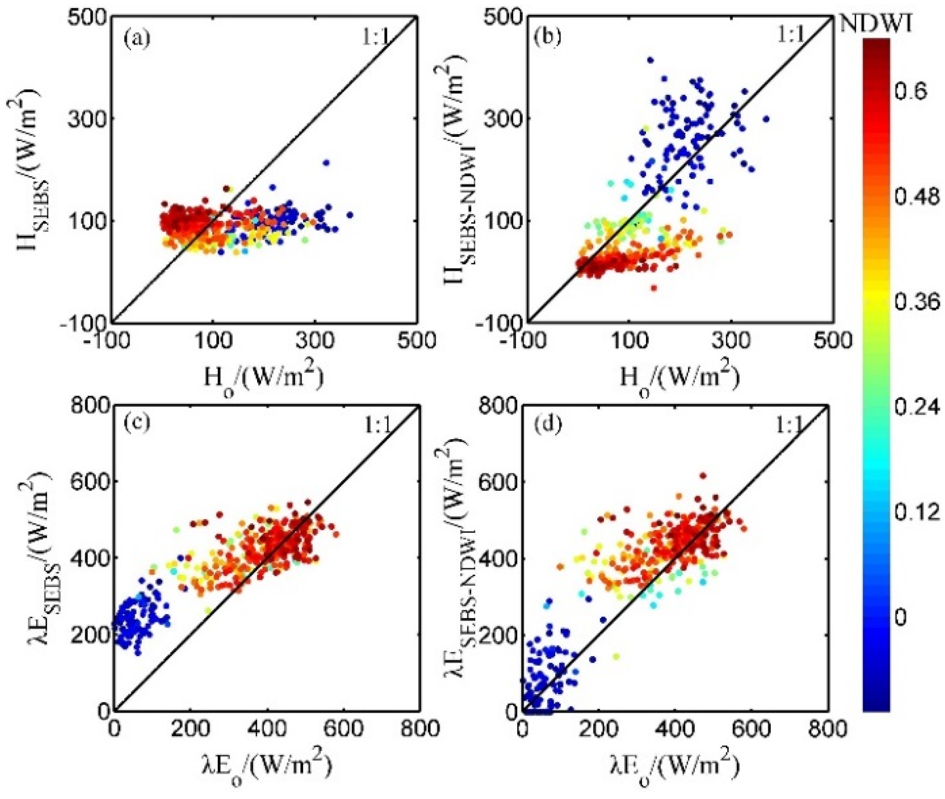
4.2. Calibration of SEBS-NDWI
| Sensible Heat Flux (H) | Latent Heat Flux (λE) | |||||||||||
|---|---|---|---|---|---|---|---|---|---|---|---|---|
| RMSE (W/m2) | BIAS (W/m2) | RMSE (W/m2) | BIAS (W/m2) | |||||||||
| Overall | NDWI ≤ 0.28 | NDWI > 0.28 | Overall | NDWI ≤ 0.28 | NDWI > 0.28 | Overall | NDWI ≤ 0.28 | NDWI > 0.28 | Overall | NDWI ≤ 0.28 | NDWI > 0.28 | |
| SEBS | 91.2 | 127.4 | 55.7 | −52.4 | −110.8 | −13.9 | 122.2 | 149.1 | 100.6 | 95.1 | 131.5 | 71.0 |
| SEBS-NDWI | 84.5 | 110.0 | 62.2 | −36.1 | −45.9 | −29.7 | 113.3 | 119.8 | 108.8 | 73.1 | 66.0 | 77.8 |
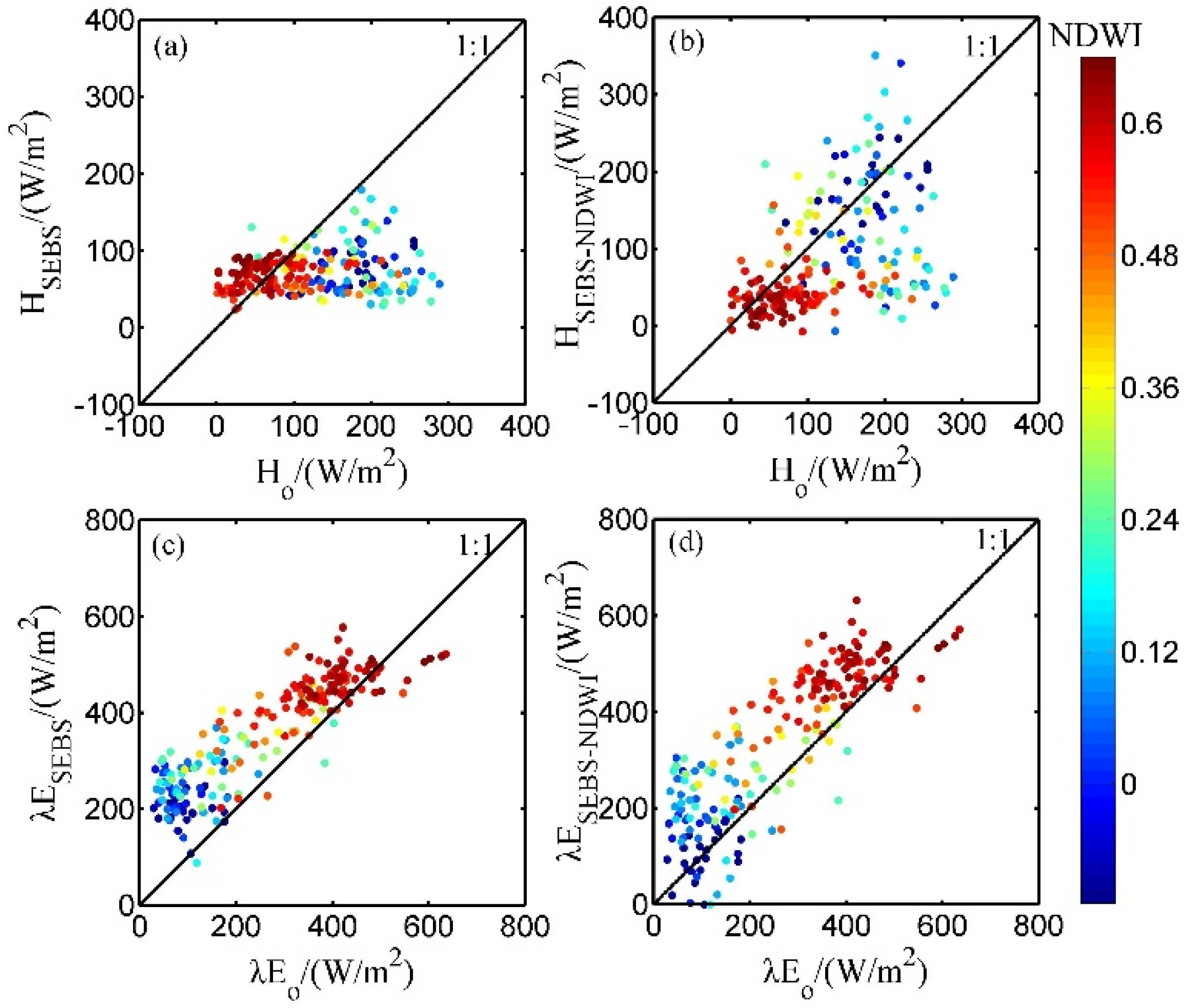
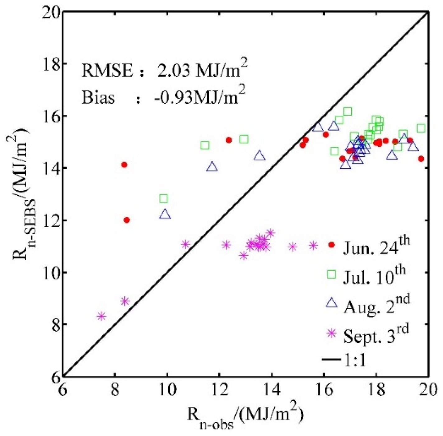
4.3. Validation of SEBS-NDWI

| Sensible Heat Flux (H) | Latent Heat Flux (λE) | |||||||||||
|---|---|---|---|---|---|---|---|---|---|---|---|---|
| RMSE (W/m2) | BIAS (W/m2) | RMSE (W/m2) | BIAS (W/m2) | |||||||||
| Overall | NDWI ≤ 0.28 | NDWI > 0.28 | Overall | NDWI ≤ 0.28 | NDWI > 0.28 | Overall | NDWI ≤ 0.28 | NDWI > 0.28 | Overall | NDWI ≤ 0.28 | NDWI > 0.28 | |
| SEBS | 84.1 | 120.7 | 65.2 | −24.9 | −105.9 | 5.5 | 117.8 | 182.4 | 81.2 | 69.4 | 166.6 | 32.8 |
| SEBS-NDWI | 79.8 | 92.5 | 74.4 | −25.3 | 45.1 | −51.8 | 84.1 | 76.6 | 86.7 | 37.6 | 23.7 | 42.8 |
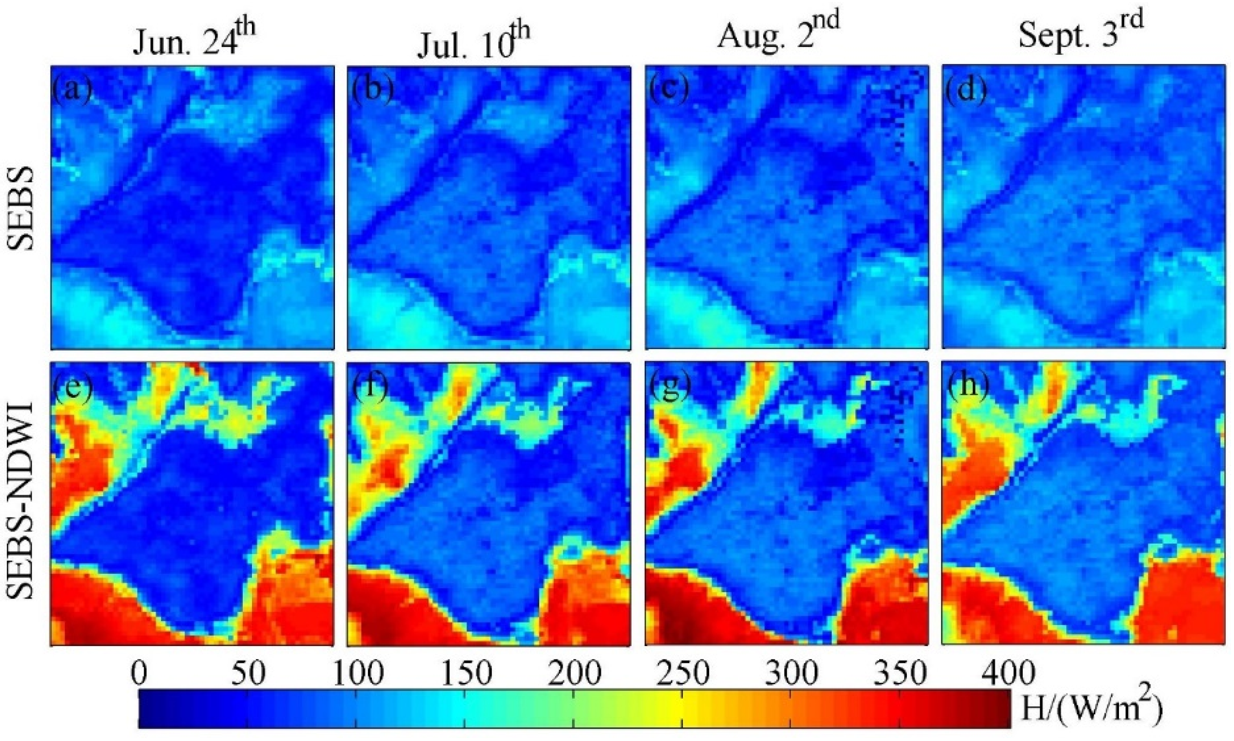
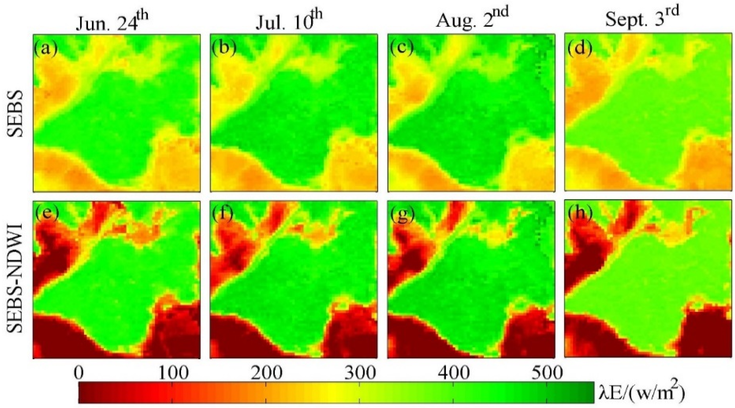
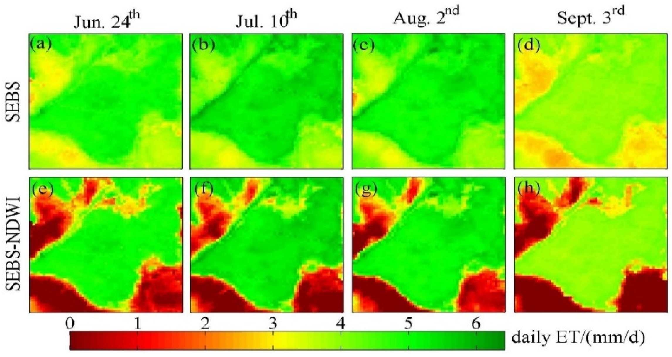
4.4. Daily ET Mapping by SEBS-NDWI


5. Conclusions
Acknowledgments
Author Contributions
Conflicts of Interest
References
- Rivas, R.; Caselles, V. A simplified equation to estimate spatial reference evaporation from remote sensing based surface temperature and local meteorological data. Remote Sens. Environ. 2003, 93, 68–76. [Google Scholar] [CrossRef]
- Courault, D.; Seguin, B.; Olioso, S. Review on estimation of evapotranspiration from remote sensing data: From empirical to numerical modeling approaches. Irrig. Drain. Syst. 2005, 19, 223–249. [Google Scholar] [CrossRef]
- Jia, Z.Z.; Liu, S.M.; Xu, Z.W.; Chen, Y.J.; Zhu, M.J. Validation of remotely sensed evapotranspiration over the hai river basin, China. J. Geophys. Res. Atmos. 2012, 117, 110–117. [Google Scholar] [CrossRef]
- Jackson, J.T.; Chen, D.; Cosh, M.; Li, F.; Anderson, M.; Walthall, C.; Doriaswamy, P.; Hunt, E.R. Vegetation water content mapping using landsat data derived normalized difference water index for corn and soybeans. Remote Sens. Environ. 2004, 92, 475–482. [Google Scholar] [CrossRef]
- Wang, K.; Wang, P.; Li, Z.; Cribb, M.; Sparrow, M. A simple method to estimate actual evapotranspiration from a combination of net radiation, vegetation index, and temperature. J. Geophys. Res. Atmos. 2007, 112, D15107. [Google Scholar] [CrossRef]
- Wang, K.; Liang, S. An improved method for estimating global evapotranspiration based on satellite determination of surface net radiation, vegetation index, temperature, and soil moisture. J. Hydrol. 2008, 9, 712–727. [Google Scholar]
- Yan, H.; Wang, S.Q.; Billesbach, D.; Oechel, W.; Zhang, J.H.; Meyers, T.; Scott, R. Global estimation of evapotranspiration using a leaf area index-based surface energy and water balance model. Remote Sens. Environ. 2012, 124, 581–595. [Google Scholar] [CrossRef]
- Cleugh, H.A.; Leuning, R.; Mu, Q.; Running, S.W. Regional evaporation estimates from flux tower and MODIS satellite data. Remote Sens. Environ. 2007, 106, 285–304. [Google Scholar] [CrossRef]
- Mu, Q.; Heinsch, F.A.; Zhao, M.; Running, S.W. Development of a global evapotranspiration algorithm based on MODIS and global meteorology data. Remote Sens. Environ. 2007, 111, 519–536. [Google Scholar] [CrossRef]
- Leuning, R.; Zhang, Y.Q.; Rajaud, A.; Cleugh, H.; Tu, K. A simple surface conductance model to estimate regional evaporation using MODIS leaf area index and the Penman-Monteith equation. Water Resour. Res. 2008, 44, W10419. [Google Scholar] [CrossRef]
- Jiang, L.; Islam, S. A methodology for estimation of surface evapotranspiration over large areas using remote sensing observations. Geophys. Res. Lett. 1999, 26, 2773–2776. [Google Scholar] [CrossRef]
- Fisher, J.B.; Tu, K.P.; Baldocchi, D.D. Global estimates of the land-atmosphere water flux based on monthly AVHRR and ISLSCP-II data, validated at 16 FLUXNET sites. Remote Sens. Environ. 2008, 112, 901–919. [Google Scholar] [CrossRef]
- Venturini, V.; Islam, S.; Rodriguez, L. Estimation of evaporative fraction and evapotranspiration from MODIS products using a complementary based model. Remote Sens. Environ. 2008, 112, 132–141. [Google Scholar] [CrossRef]
- García, M.; Sandholt, I.; Ceccato, P.; Ridler, M.; Mougin, E.; Kergoat, L.; Morillas, L.; Timouk, F.; Fensholt, R.; Domingo, F. Actual evapotranspiration in drylands derived from in situ and satellite data: Assessing biophysical constraints. Remote Sens. Environ. 2013, 131, 103–118. [Google Scholar] [CrossRef]
- Bastiaanssen, W.G.M.; Menenti, M.; Feddes, R.A.; Holtslag, A.A.M. A remote sensing surface energy balance algorithm for land (SEBAL)—1. Formulation. J. Hydrol. 1998, 213, 198–212. [Google Scholar] [CrossRef]
- Roerink, G.J.; Su, Z.; Menenti, M. S-SEBI: A simple remote sensing algorithm to estimate the surface energy balance. Phys. Chem. Earth B Hydrol. Oceans Atmos. 2000, 25, 147–157. [Google Scholar] [CrossRef]
- Su, Z. The Surface Energy Balance System (SEBS) for estimation of turbulent heat fluxes. Hydrol. Earth Syst. Sci. 2002, 6, 85–99. [Google Scholar] [CrossRef]
- Allen, R.G.; Tasumi, M.; Trezza, R. Satellite-based energy balance for mapping evapotranspiration with internalized calibration (METRIC)-Model. J. Irrig. Drain. Eng. ASCE 2007, 133, 380–394. [Google Scholar] [CrossRef]
- Norman, J.M.; Kustas, W.P.; Humes, K.S. Source approach for estimating soil and vegetation energy fluxes in observations of directional radiometric surface temperature. Agric. For. Meteorol. 1995, 77, 263–293. [Google Scholar] [CrossRef]
- Lion, Y.A.; Kar, S.K. Evapotranspiration Estimation with Remote Sensing and Various Surface Energy Balance algorithms—A review. Energies 2014, 7, 2821–2847. [Google Scholar]
- Caparrini, F.; Castelli, F.; Entekhabi, D. Estimation of surface turbulent fluxes through assimilation of radiometric surface temperature sequences. J. Hydrometeorol. 2004, 5, 145–159. [Google Scholar] [CrossRef]
- Huang, C.L.; Li, X.; Wang, J.M.; Gu, J. Assimilation of remote sensing data products into common land model for evapotranspiration forecasting. In Proceedings of the 8th International Symposium on Spatial Accuracy Assessment in Natural Resources and Environmental Sciences, Shanghai, China, 25–27 June 2008.
- Xu, T.R.; Liang, S.L.; Liu, S.M.; Zhu, X.F.; Tao, X. Estimating turbulent fluxes through assimilation of geostationary operational environmental satellites data using ensemble Kalman filter. J. Geophys. Res. 2011, 116, D09109. [Google Scholar] [CrossRef]
- Tang, R.; Li, Z.L.; Jia, Y.; Li, C.; Sun, X.; Kustas, W.P.; Anderson, M.C. An intercomparison of three remote sensing-based energy balance models using Large Aperture Scintillometer measurements over a wheat-corn production region. Remote Sens. Environ. 2011, 115, 3187–3202. [Google Scholar] [CrossRef]
- Wang, Y.Y.; Li, X.; Tang, S.H. Validation of the SEBS-derived sensible heat for FY3A/VIRR and TERRA/MODIS over an alpine grass region using LAS measurements. Int. J. Appl. Earth Obs. 2013, 23, 226–233. [Google Scholar] [CrossRef]
- Jia, L.; Su, Z.; Bart, H.; Menenti, M.; Moene, A.; de Bruin, H.A.R.; Javier, B.Y.J.; Ibanez, M.; Cuesta, A. estimation of sensible heat flux using the Surface Energy Balance System(SEBS) and ATSR measurements. Phys. Chem. Earth 2003, 28, 75–88. [Google Scholar] [CrossRef]
- Ma, W.Q.; Ma, Y.M.; Hu, Z.Y.; Su, Z.; Wang, J.M.; Ishikawa, H. Estimation surface fluxes over middle and upper streams of the Heihe River Basin with ASTER imagery. Hydrol. Earth Syst. Sci. 2011, 15, 1403–1413. [Google Scholar] [CrossRef]
- Kwast, J.; Timmermans, W.; Gieske, A.; Su, Z.; Olioso, A.; Jia, L.; Elbers, J.; Karssenberg, D.; de Jong, S. Evaluation of the Surface Energy Balance System (SEBS) applied to ASTER imagery with flux-measurements at the SPARC 2004 site (Barrax, Spain). Hydrol. Earth Syst. Sci. 2009, 13, 1337–1347. [Google Scholar] [CrossRef]
- Elhag, M.; Psilovikos, A.; Manakos, I.; Perakis, K. Application of the SEBS water balance model in estimating daily evapotranspiration and evaporative fraction from remote sensing data over the Nile Delta. Water Resour. Manag. 2011, 25, 2731–2742. [Google Scholar] [CrossRef]
- Alkhaier, F.; Su, Z.; Flerchinger, G.N. Reconnoitering the effect of shallow groundwater on land surface temperature and surface energy balance using MODIS and SEBS. Hydrol. Earth Syst. Sci. 2012, 16, 1833–1844. [Google Scholar] [CrossRef]
- Gokmen, M.; Vekerdy, Z.; Verhoef, A.; Verhoef, A.; Batelaan, O.; Tol, C. Integration of soil moisture in SEBS for improving evapotranspiration estimation under water stress conditions. Remote Sens. Environ. 2012, 121, 261–274. [Google Scholar] [CrossRef]
- Pardo, N.; Sánchez, M.L.; Timmermans, J.; Su, Z.; Pérez, I.A.; García, M. SEBS validation in a Spanish rotating crop. Agric. For. Meteorol. 2014, 195, 132–142. [Google Scholar] [CrossRef]
- Miralles, D.G.; Holmes, T.R.H.; Jeu, R.A.M.; Gash, J.H.; Meesters, A.; Dolman, A.J. Global land-surface evaporation estimated from satellite-based observations. Hydrol. Earth Syst. Sci. 2011, 15, 453–469. [Google Scholar] [CrossRef]
- Campos, I.; Villodre, J.; Carrara, A.; Calera, A.; Caleraa, A. Remote sensing-based soil water balance to estimate Mediterranean holm oak savanna (dehesa) evapotranspiration under water stress. J. Hydrol. 2013, 494, 1–9. [Google Scholar] [CrossRef]
- Ding, R.H.; Kang, S.Z.; Li, F.H.; Zhang, Y.Q.; Tong, L. Evapotranspiration measurement and estimation using modified Priestley-Taylor model in an irrigated maize field with mulching. Agric. For. Meteorol. 2013, 168, 140–148. [Google Scholar] [CrossRef]
- Ma, Y.F.; Liu, S.M.; Zhang, F.; Zhou, J.; Jia, Z.Z.; Song, L.S. Estimations of regional surface energy fluxes over heterogeneous oasis-desert surfaces in the middle reaches of the Heihe River during HiWATER-MUSOEXE. IEEE Geosci. Remote Sens. Lett. 2015, 12, 671–675. [Google Scholar]
- Huang, C.L.; Li, Y.; Lu, L.; Gu, J. Estimation of surface fluxes under drought water stress conditions based on remotely sensed data. Adv. Water Sci. 2014, 25, 181–188. (In Chinese) [Google Scholar]
- Li, X.; Li, X.W.; Li, Z.; Ma, M.; Wang, J.; Xiao, Q.; Liu, Q.; Che, T.; Chen, E.; Yan, G.; et al. Watershed allied telemetry experimental research. J. Geophys. Res. Atmos. 2009, 114, D22103. [Google Scholar] [CrossRef]
- Wu, X.J.; Zhou, J.; Wang, H.J.; Li, Y.; Zhong, B. Evaluation of irrigation water use efficiency using remote sensing in the middle reach of the Heihe river, in the semi-arid northwestern China. Hydrol. Process. 2015, 29, 2243–2257. [Google Scholar] [CrossRef]
- Li, X.; Cheng, G.; Liu, S.; Xiao, Q.; Ma, M.; Jin, R.; Che, T.; Liu, Q.; Wang, W.; Qi, Y.; et al. Heihe watershed allied telemetry experimental research (HiWATER): Scientific objectives and experimental design. Bull. Am. Meteorol. Soc. 2013, 94, 1145–1160. [Google Scholar] [CrossRef]
- Seneviratne, S.I.; Corti, T.; Davin, E.L.; Hirschi, M.; Jaeger, E.B.; Lehner, I.; Orlowsky, B.; Teuling, A.J. Investigating soil moisture-climate interactions in a changing climate: A review. Earth-Sci. Rev. 2010, 99, 125–161. [Google Scholar] [CrossRef]
- Xu, Z.W.; Liu, S.M.; Li, X.; Shi, S.J.; Wang, J.M.; Zhu, Z.L.; Xu, T.R.; Wang, W.; Ma, M. Intercomparison of surface energy flux measurement systems used during the HiWATER-MUSOEXE. J. Geophys. Res. 2013, 118, 13140–13157. [Google Scholar] [CrossRef]
- Liu, S.M.; Xu, Z.W.; Wang, W.Z.; Bai, J.; Jia, Z.; Zhu, M.; Wang, J.M. A comparison of eddy-covariance and large aperture scintillometer measurements with respect to the energy balance closure problem. Hydrol. Earth Syst. Sci. 2011, 15, 1291–1306. [Google Scholar] [CrossRef]
- Liu, S.M.; Xu, Z.W.; Zhu, Z.L.; Jia, Z.Z.; Zhu, M.J. Measurements of evapotranspiration from eddy-covariance systems and large aperture scintillometers in the Hai River Basin, China. J. Hydrol. 2013, 487, 24–38. [Google Scholar] [CrossRef]
- Twine, T.E.; Kustas, W.P.; Norman, J.M.; Cook, D.R.; Houser, P.R. Correcting eddy-covariance flux underestimation over a grassland. Agric. For. Meteorol. 2000, 103, 279–300. [Google Scholar] [CrossRef]
- Gao, B.C. NDWI-A normalized difference water Index for remote sensing of vegetation liquid water from space. Remote Sens. Environ. 1996, 58, 257–266. [Google Scholar] [CrossRef]
- Chen, D.Y.; Huang, J.F.; Thomas, J.J. Vegetation water content estimation for corn and soybeans using spectral indices derived from MODIS near and short-wave infrared bands. Remote Sens. Environ. 2005, 98, 225–236. [Google Scholar] [CrossRef]
- Su, Z.; Schmugge, T.; Kustas, W.P.; Massman, W.J. An evaluation of two models for estimation of the roughness height for heat transfer between the land surface and the atmosphere. J. Appl. Meteorol. 2001, 40, 1933–1951. [Google Scholar] [CrossRef]
- Brutsaert, M. Evaporation into the Atmosphere: Theory, History and Applications; Springer: Hingham, MA, USA, 1982. [Google Scholar]
- Nichols, W.E.; Cuenca, R.H. Evaluation of the evaporative fraction for parameterization of the surface energy balance. Water Resour. Res. 1993, 29, 3681–3690. [Google Scholar] [CrossRef]
- Crago, R.; Brutsaert, W. Daytime evaporation and the self-preservation of the evaporative fraction and the Bowen ratio. J. Hydrol. 1996, 178, 241–255. [Google Scholar] [CrossRef]
- Hoedjes, J.C.B.; Chehbouni, A.; Jacob, F.; Ezzahar, J.; Boulet, G. Deriving daily evapotranspiration from remotely sensed instantaneous evaporative fraction over olive orchard in semi-arid Morocco. J. Hydrol. 2008, 354, 53–64. [Google Scholar] [CrossRef]
- Delogu, E.; Boulet, G.; Olioso, A.; Coudert, B.; Chirouze, J.; Ceschia, E.; le Dantec, V.; Marloie, O.; Chehbouni, G.; Lagouarde, J.-P. Reconstruction of temporal variations of evapotranspiration using instantaneous estimates at the time of satellite overpass. Hydrol. Earth Syst. Sci. 2013, 16, 2995–3010. [Google Scholar] [CrossRef] [Green Version]
- Hurtado, E.; Sobrino, J.A. Daily net radiation estimated from air temperature and NOAA-AVHRR data: A case study for Iberian Penisula. Int. J. Remote Sens. 2001, 22, 1521–1533. [Google Scholar] [CrossRef]
- Tian, H. Remote-Sensed Estimates of Evapotranspiration over A Complex Terrain of the Inland Hei River Basin; Cold and Arid Regions Environment and Engineering Research Insitute, Chinese Academy of Sciences: Lanzhou, China, 2008. (In Chinese) [Google Scholar]
- Brunt, D. Physical and Dynamical Meteorology, 2nd ed.; Cambridge University Press: New York, NY, USA, 1939. [Google Scholar]
- Carlson, T.N.; Ripley, D.A. On the relation between NDVI, fractional vegetation cover, and leaf area index. Remote Sens. Environ. 1997, 62, 241–252. [Google Scholar] [CrossRef]
- Liang, S.L. Narrowband to broadband conversions of land surface albedo I: Algorithms. Remote Sens. Environ. 2001, 76, 213–238. [Google Scholar] [CrossRef]
- Sobrino, J.A.; Caselles, V.; Becker, F. Significance of the remote sensed thermal infrared measurements obtained over a citrus orchard. ISPRS J. Photogramm. 1990, 44, 343–354. [Google Scholar] [CrossRef]
- Valor, E.; Caselles, V. Mapping land surface emissivity from NDVI: Application to European, African and South American areas. Remote Sens. Environ. 1996, 57, 167–184. [Google Scholar] [CrossRef]
- Duan, Q.Y.; Sorooshian, S.; Gupta, V. Effective and efficient global optimization for conceptual rain fall run off models. Water Resour. Res. 1992, 28, 1015–1031. [Google Scholar] [CrossRef]
- Crow, W.T.; Wood, E.F. Impact of soil moisture aggregation on surface energy flux prediction during SGP’97. Geophys. Res. Lett. 2002, 29, 1008. [Google Scholar] [CrossRef]
- Ronda, R.J.; van den Hurk, B.J.J.M.; Holtslag, A.A.M. Spatial heterogeneity of the soil moisture content and its impact on surface flux densities and near-surface meteorology. J. Hydrometeorol. 2002, 3, 556–570. [Google Scholar] [CrossRef]
- He, L.; Ivanov, V.Y.; Bohrer, G.; Maurer, K.D.; Vogel, C.S.; Moghaddam, M. Effects of fine-scale soil moisture and canopy heterogeneity on energy and water fluxes in a northern temperate mixed forest. Agric. For. Meteorol. 2014, 184, 243–256. [Google Scholar] [CrossRef]
- Xu, T.R.; Liu, S.M.; Lu, X.; Chen, Y.J.; Jia, Z.Z.; Xu, Z.W.; Nielson, J. Temporal upscaling and reconstruction of thermal remotely sensed instantaneous evapotranspiration. Remote Sens. 2015, 7, 3400–3425. [Google Scholar] [CrossRef]
- Guerschman, J.P.; van Dijk, A.I.J.M.; Mattersdorf, G.; Beringer, J.; Hutley, L.B.; Leuning, R.; Pipunic, P.C.; Sherman, B.S. Scaling of potential evapotranspiration with MODIS data reproduces flux observations and catchment water balance observations across Australia. J. Hydrol. 2009, 369, 107–119. [Google Scholar] [CrossRef]
© 2015 by the authors; licensee MDPI, Basel, Switzerland. This article is an open access article distributed under the terms and conditions of the Creative Commons by Attribution (CC-BY) license (http://creativecommons.org/licenses/by/4.0/).
Share and Cite
Huang, C.; Li, Y.; Gu, J.; Lu, L.; Li, X. Improving Estimation of Evapotranspiration under Water-Limited Conditions Based on SEBS and MODIS Data in Arid Regions. Remote Sens. 2015, 7, 16795-16814. https://doi.org/10.3390/rs71215854
Huang C, Li Y, Gu J, Lu L, Li X. Improving Estimation of Evapotranspiration under Water-Limited Conditions Based on SEBS and MODIS Data in Arid Regions. Remote Sensing. 2015; 7(12):16795-16814. https://doi.org/10.3390/rs71215854
Chicago/Turabian StyleHuang, Chunlin, Yan Li, Juan Gu, Ling Lu, and Xin Li. 2015. "Improving Estimation of Evapotranspiration under Water-Limited Conditions Based on SEBS and MODIS Data in Arid Regions" Remote Sensing 7, no. 12: 16795-16814. https://doi.org/10.3390/rs71215854