
Optimization of a Semi-Analytical Algorithm for Multi-Temporal Water Quality Monitoring in Inland Waters with Wide Natural Variability

Abstract
:
1. Introduction
2. Theoretical Background
2.1. Deriving Reflectance and Accounting for the Air–Water Interface
2.2. Relating Remote Sensing Reflectance to Inherent Optical Properties
2.3. Modeling Inherent Optical Properties
2.4. Inversion of Reflectance
3. Materials and Methods
3.1. Study Area
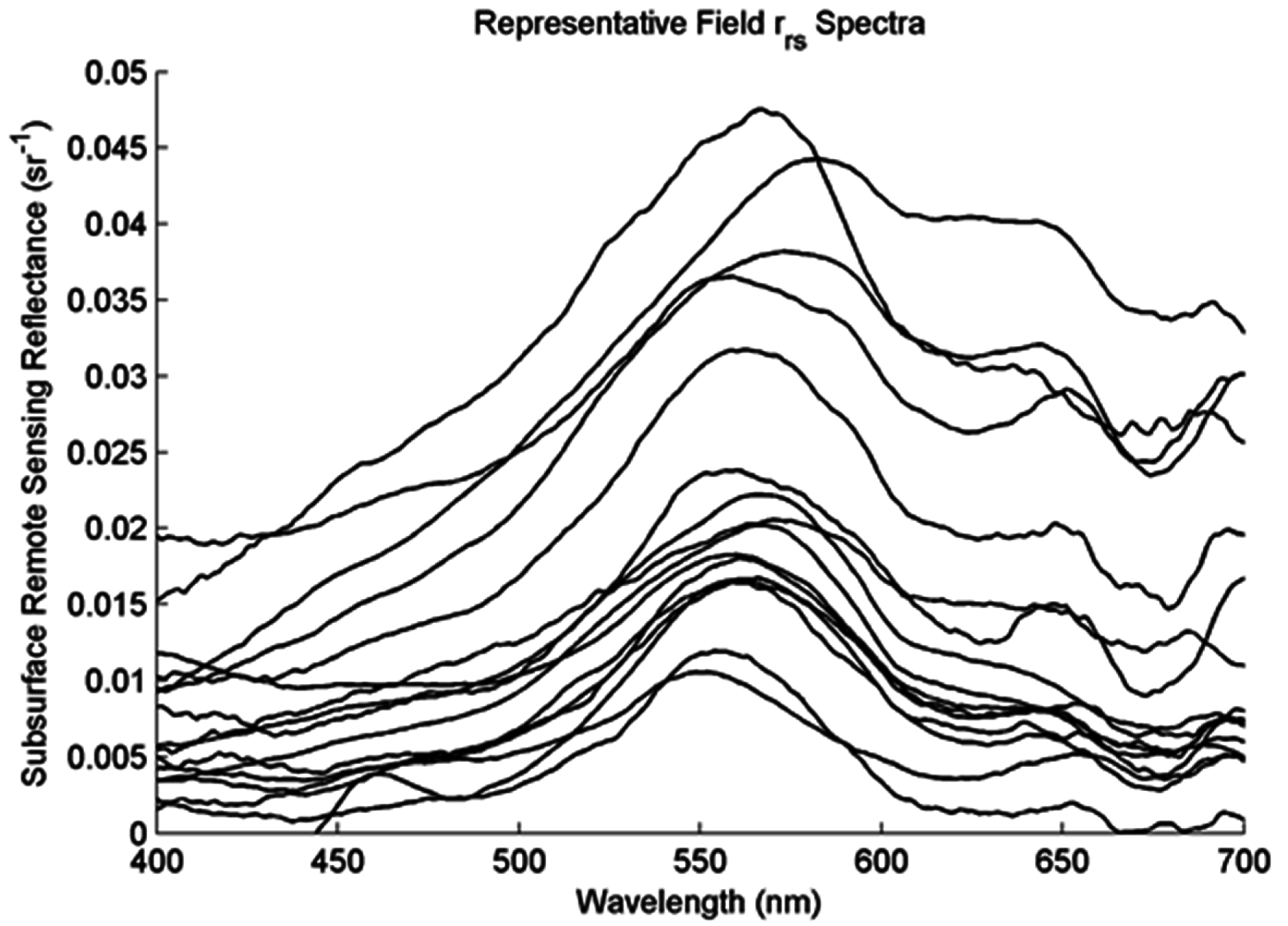
3.2. Remote Sensing Reflectance Measurements

3.3. Constituent Concentrations

3.4. Water Constituent SIOPs
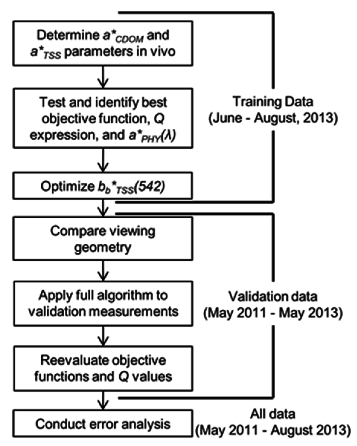
3.5. Bio-Optical Algorithm Parameterization

| Initial Parameterization | ||||
|---|---|---|---|---|
| Variable | Value | Source | Constituent | Range |
| YTSS | 0.681 | [19] | Chl-a | 0–150 mg∙m−3 |
| SCDOM | 0.014 | This study | ||
| STSS | 0.007 | This study | TSS | 0–30 g∙m−3 |
| aCDOM(λ0) | 440 nm | [12] | ||
| aTSS(λ0) | 440 nm | [12] | CDOM | 0–5 m−1 |
| bbTSS λ0 | 542 nm | [19] | ||
| a*PHY(λ) | Variable | This study | ||
| a*TSS(λ0) | 0.06–0.15 m2∙g−1 | This study | ||
| a*CDOM(λ0) | 1 | N/A | ||
| bb*TSS(λ0) | 0.054 m2∙g−1 | [19] | ||
| Start wavelength | 400 nm | N/A | ||
| End wavelength | 725 nm | N/A | ||
| End wavelength | 725 nm | N/A | ||

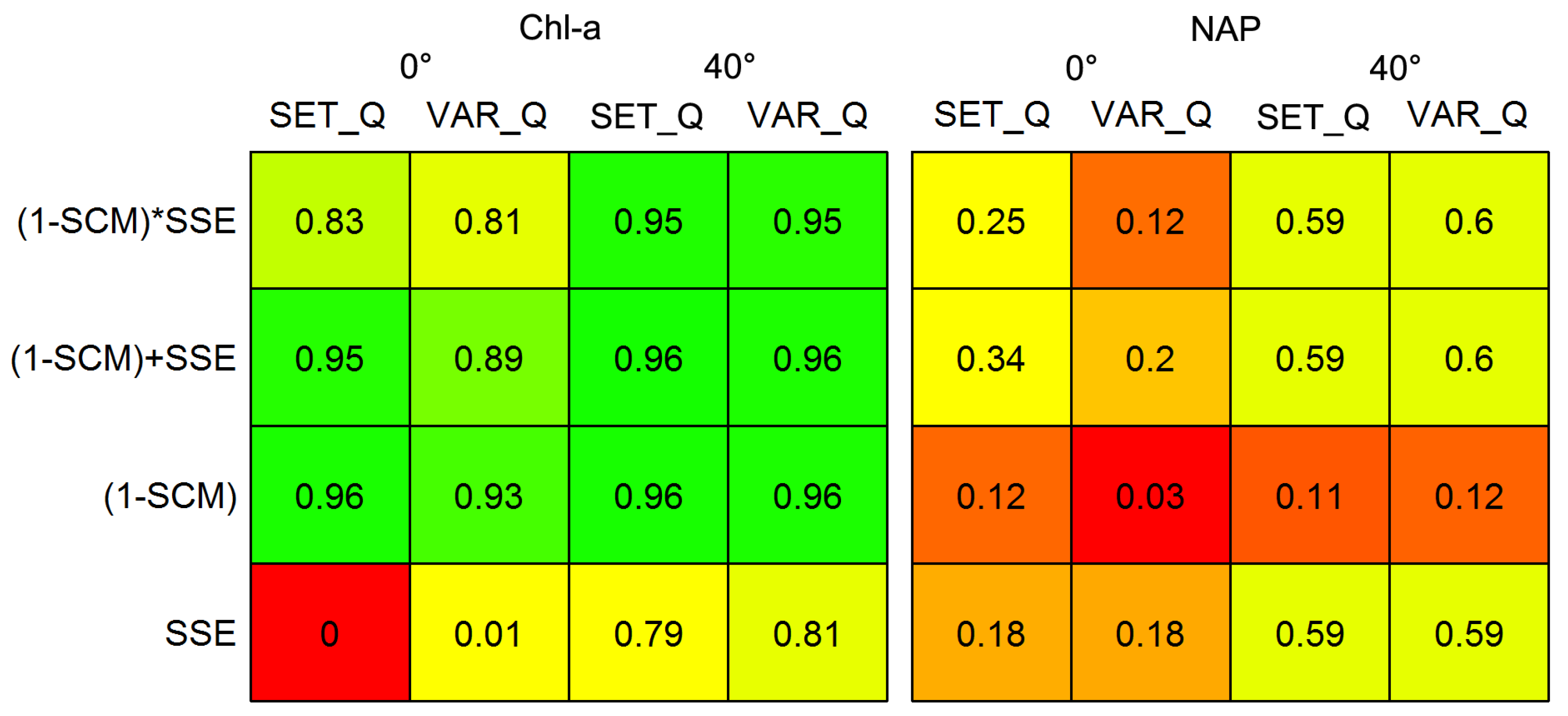
| Abbreviation | Expression for Q |
|---|---|
| SET_Q | Q = 3.5 [20] |
| VAR_Q | [11] |
3.6. Statistical Analysis
4. Results and Discussion
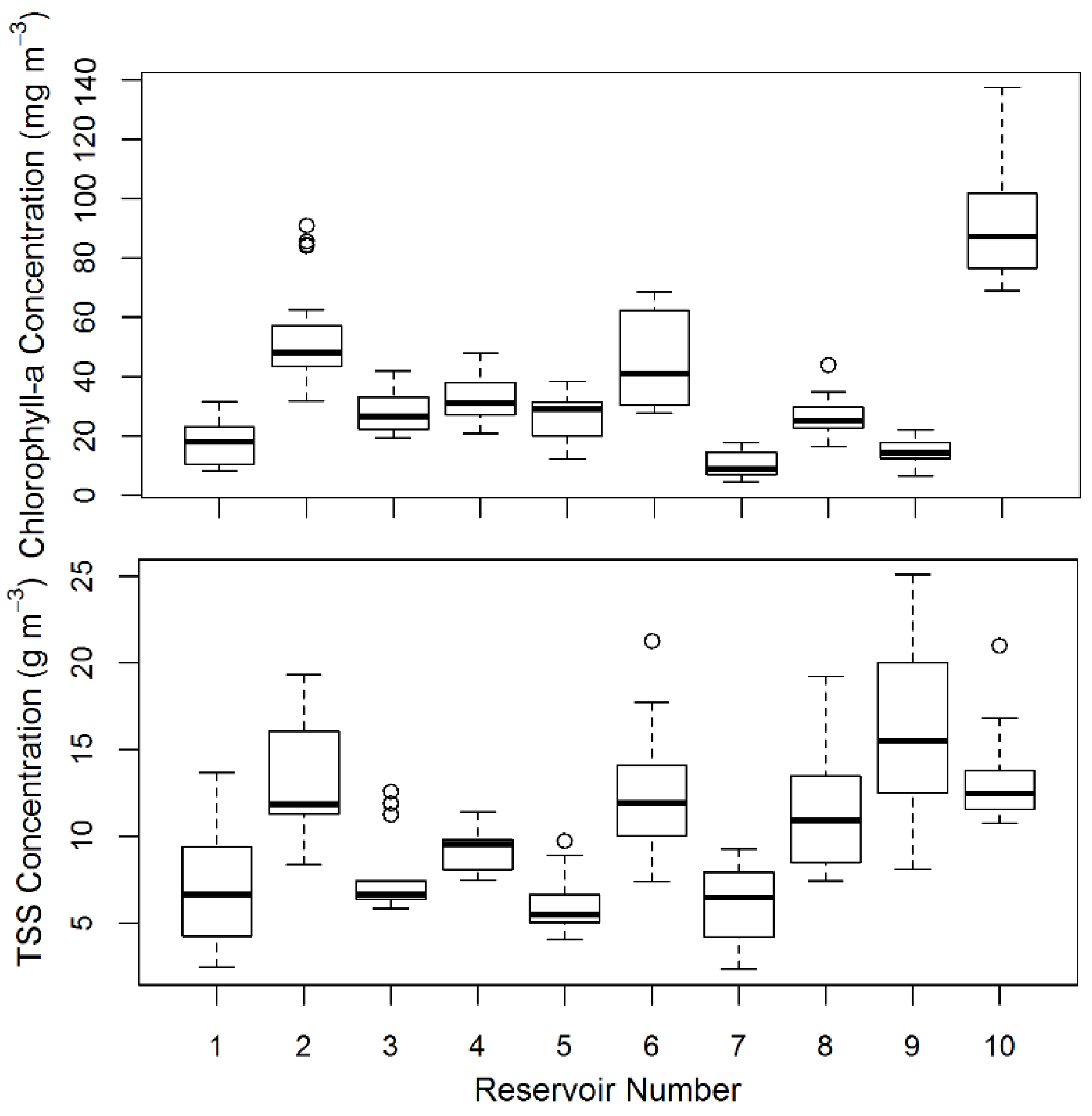
4.1. Characterization of Reservoirs
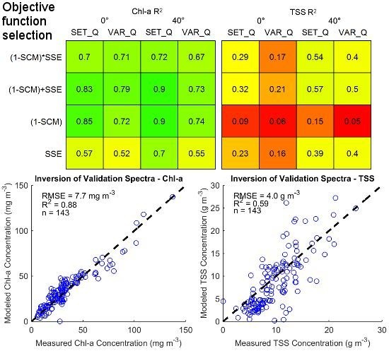
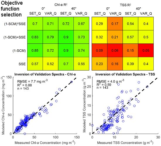
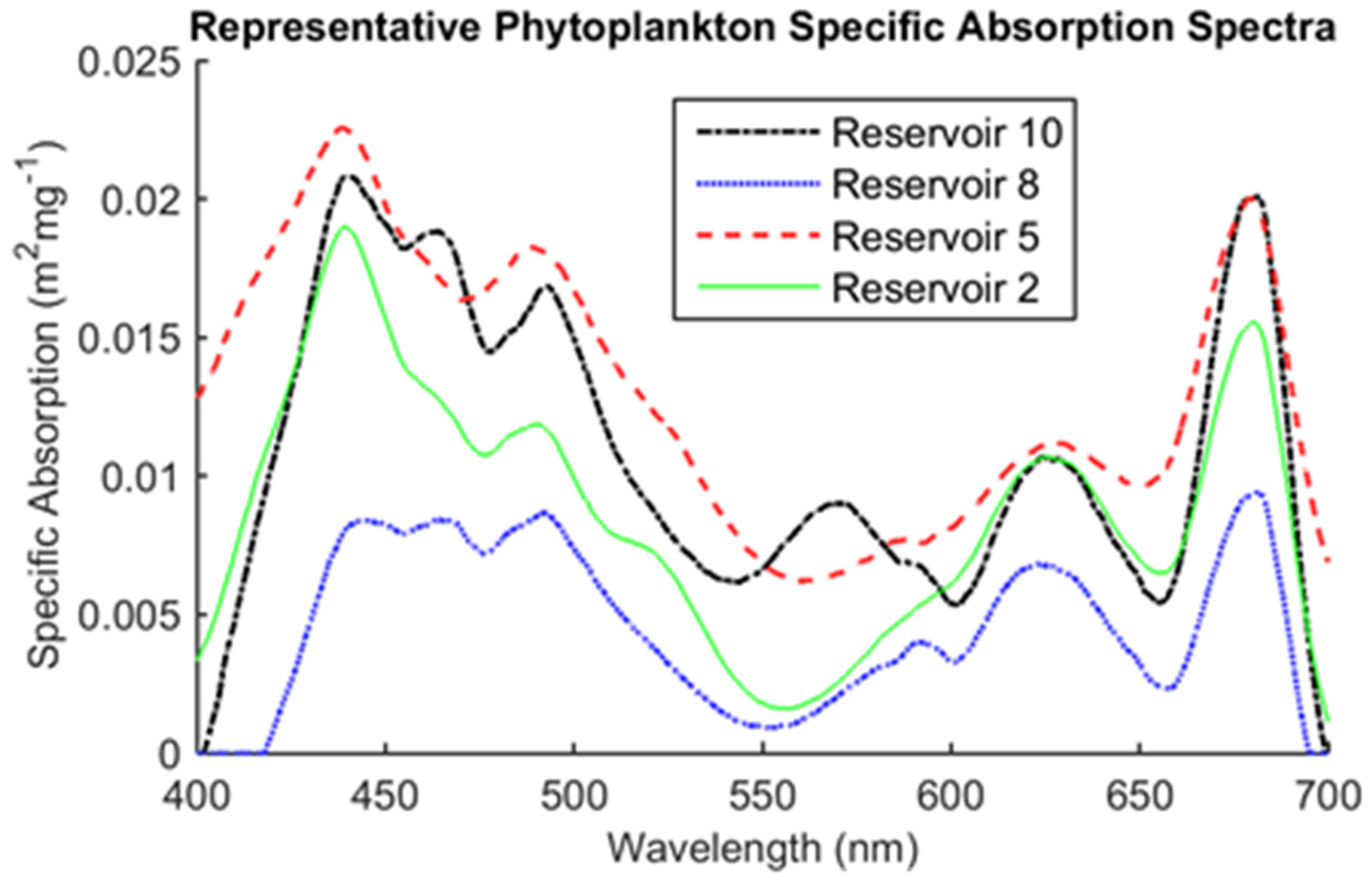
4.2. Parameterizing Objective Function, Q, a*PHY(λ), and bb*TSS(542)

4.3. Comparison of View Angles
| Final Parameterization | ||
|---|---|---|
| Variable | Value | Source |
| YTSS | 0.681 | [19] |
| SCDOM | 0.014 | This study |
| STSS | 0.007 | This study |
| aCDOM λ0 | 440 nm | [12] |
| aTSS λ0 | 440 nm | [12] |
| bbTSS λ0 | 542 nm | [19] |
| a*PHY | Spectrum (Figure 6) | This study |
| a*TSS | 0.06–0.3 m2∙g−1 | This study |
| a*CDOM | 1 | N/A |
| bb*TSS | 0.0147 m2∙g−1 | This study |
| Start wavelength | 400 nm | N/A |
| End wavelength | 725 nm | N/A |

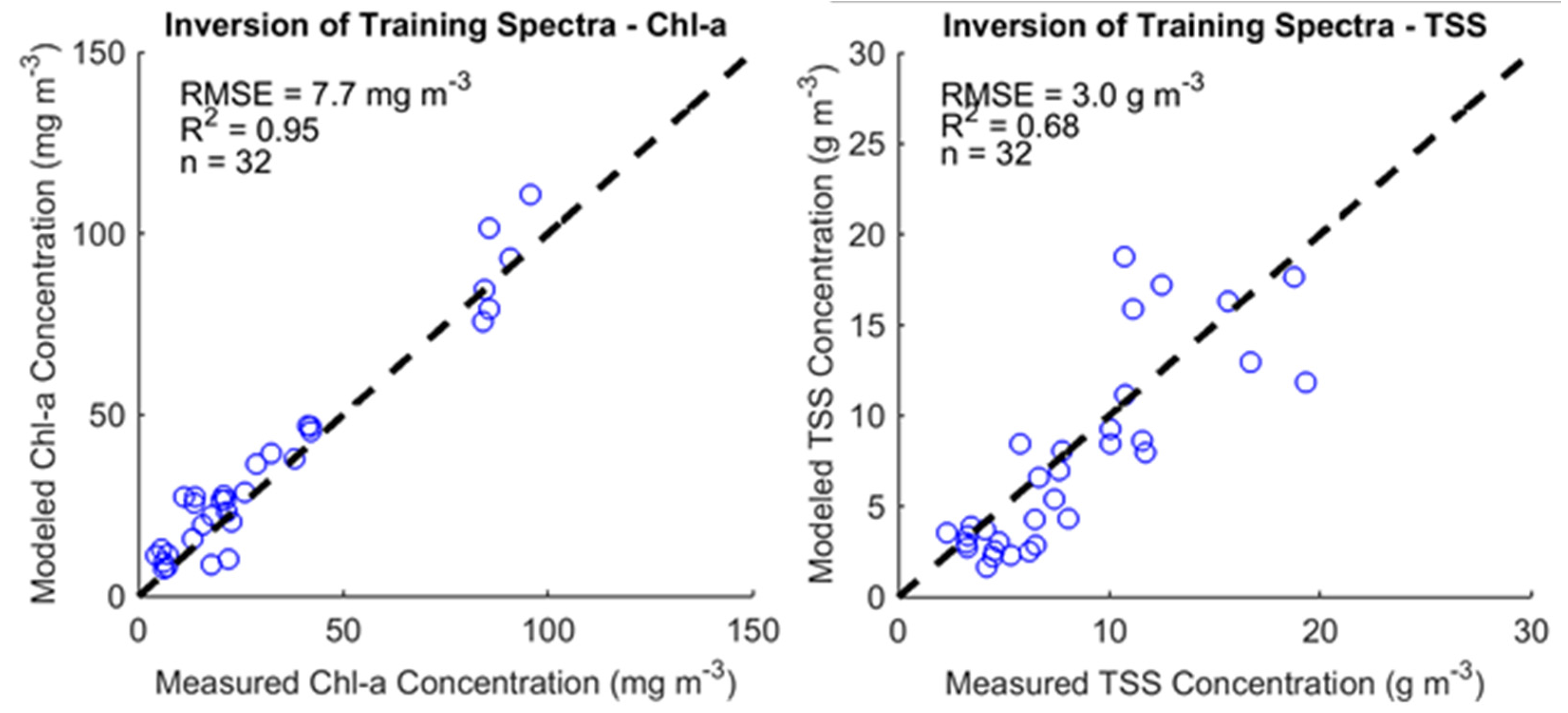
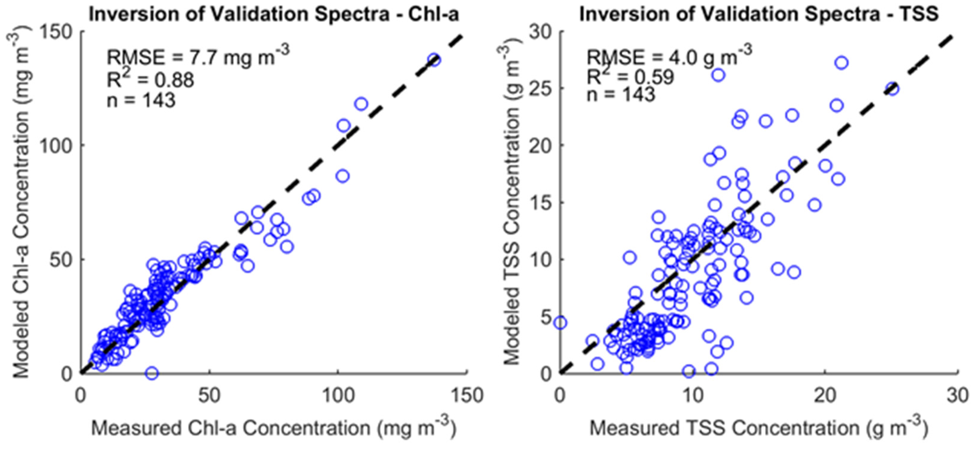
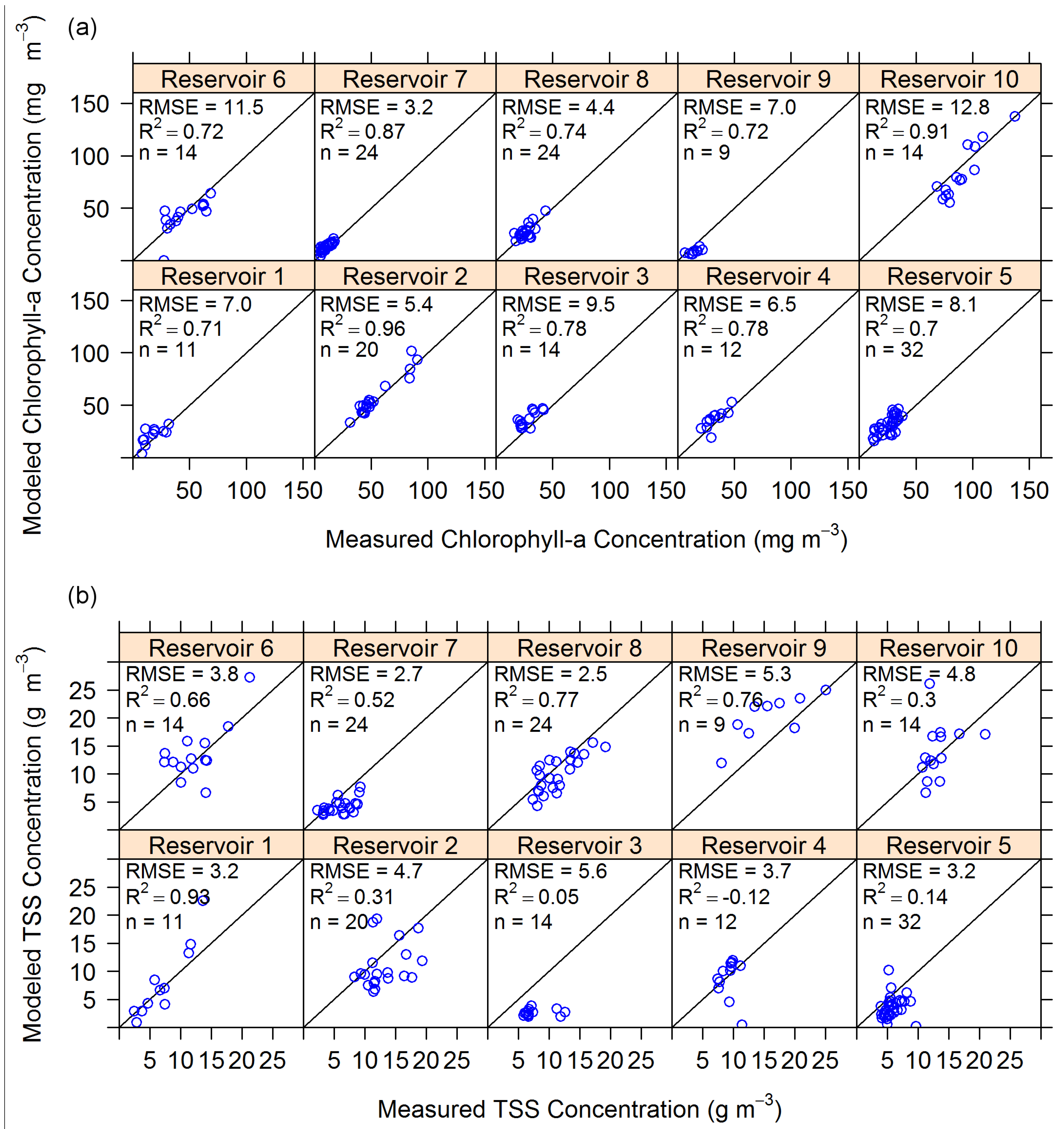
4.4. Applying SA Algorithm to All Available Data

| Chl-a RMSE (mg∙m−3) | |||
| Viewing Angle | Optimized Algorithm—Training Data | Optimized Algorithm—Validation Data | Optimized Algorithm—All Data |
| 0° | 9.2 | 10.5 | 10.3 |
| 40° | 7.7 | 7.7 | 7.7 |
| TSS RMSE (g∙m−3) | |||
| Viewing Angle | Optimized Algorithm—Training data | Optimized Algorithm—Validation data | Optimized Algorithm—All data |
| 0° | 6.3 | 5.2 | 5.4 |
| 40° | 3.0 | 4.0 | 3.9 |
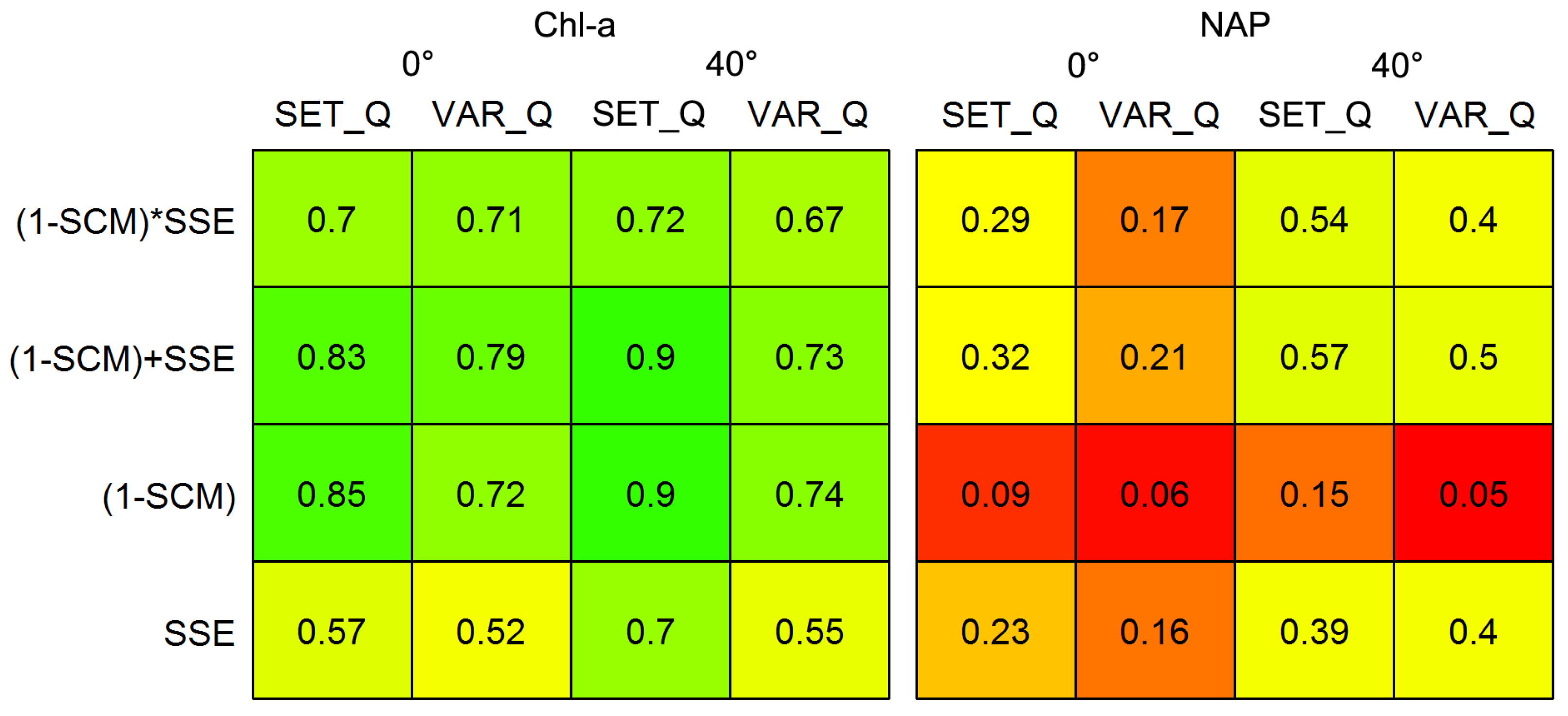
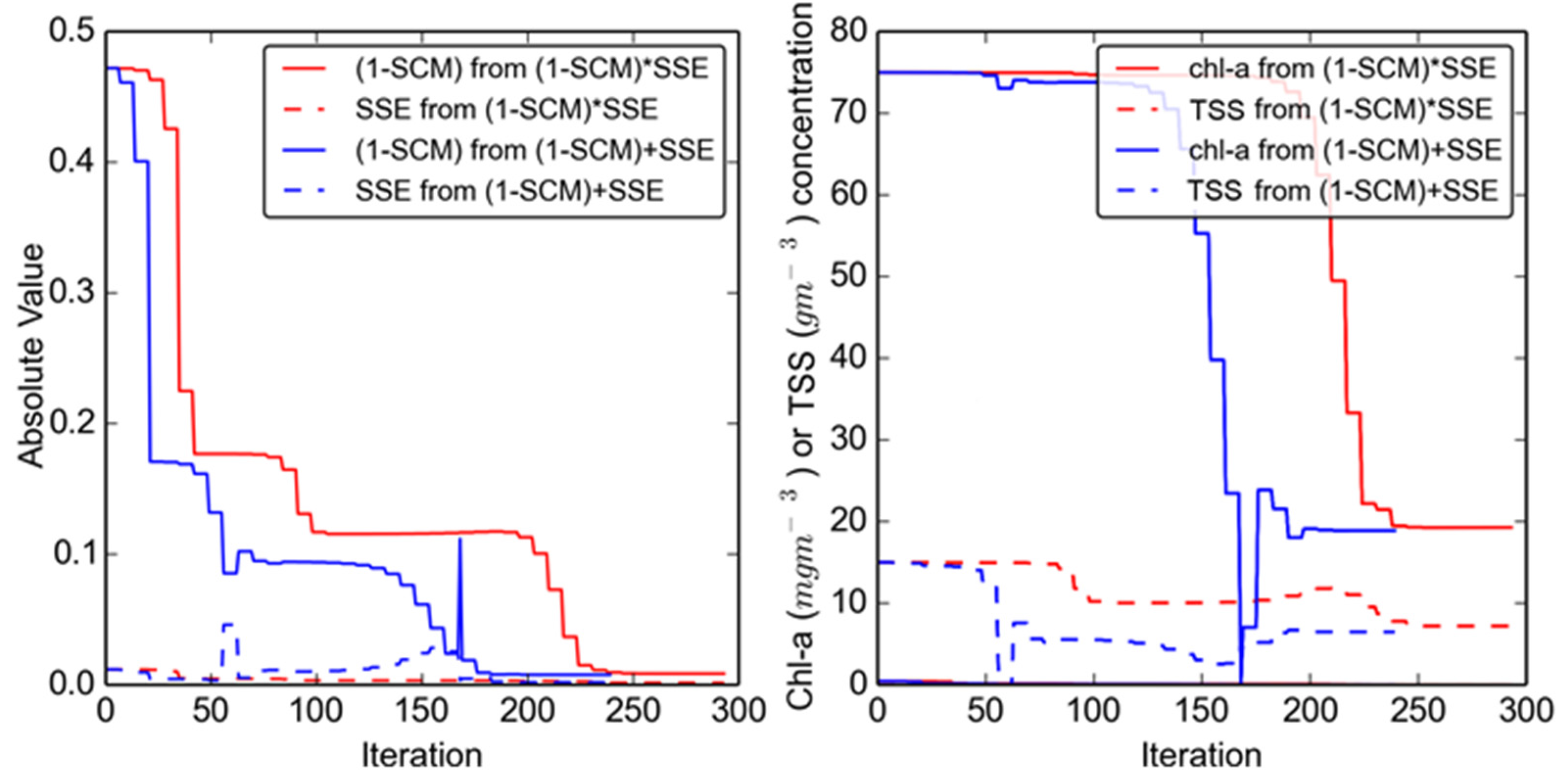
4.5. Comparison of Objective Functions and Q Expressions
4.6. Analysis of Error
4.6.1. Error from Algorithm Parameterization
| Model Number | Dependent Variable | Independent Variables 1 | R2 | Adj. R2 |
|---|---|---|---|---|
| 1 | Chl-a error | Reservoir | 0.25 | 0.21 |
| 2 | TSS error | Reservoir | 0.15 | 0.1 |
| 3 | Chl-a error | Reservoir + [Chl-a] + Reservoir × [Chl-a] | 0.34 | 0.26 |
| 4 | TSS error | Reservoir + [TSS] + Reservoir × [TSS] | 0.39 | 0.31 |
| 5 | Chl-a error | Reservoir + Month 2 + Reservoir × Month 2 | 0.32 | 0.23 |
| 6 | TSS error | Reservoir + Month 2 + Reservoir × Month 2 | 0.24 | 0.14 |
| 7 | TSS error | Month 2, 3 | 0.6 | 0.58 |
| 8 | Chl-a errorreplicate4 | Reservoir + σspectral + Reservoir × σspectral | 0.46 | 0.39 |
| 9 | Chl-a errorreplicate4 | Reservoir | 0.3 | 0.27 |
| 10 | Chl-a error | Reservoir + σspectral + Reservoir × σspectral | 0.3 | 0.21 |
| 11 | TSS errorreplicate4 | Reservoir + σspectral + Reservoir × σspectral | 0.22 | 0.12 |
4.6.2. Error from Optical Parameter Variability
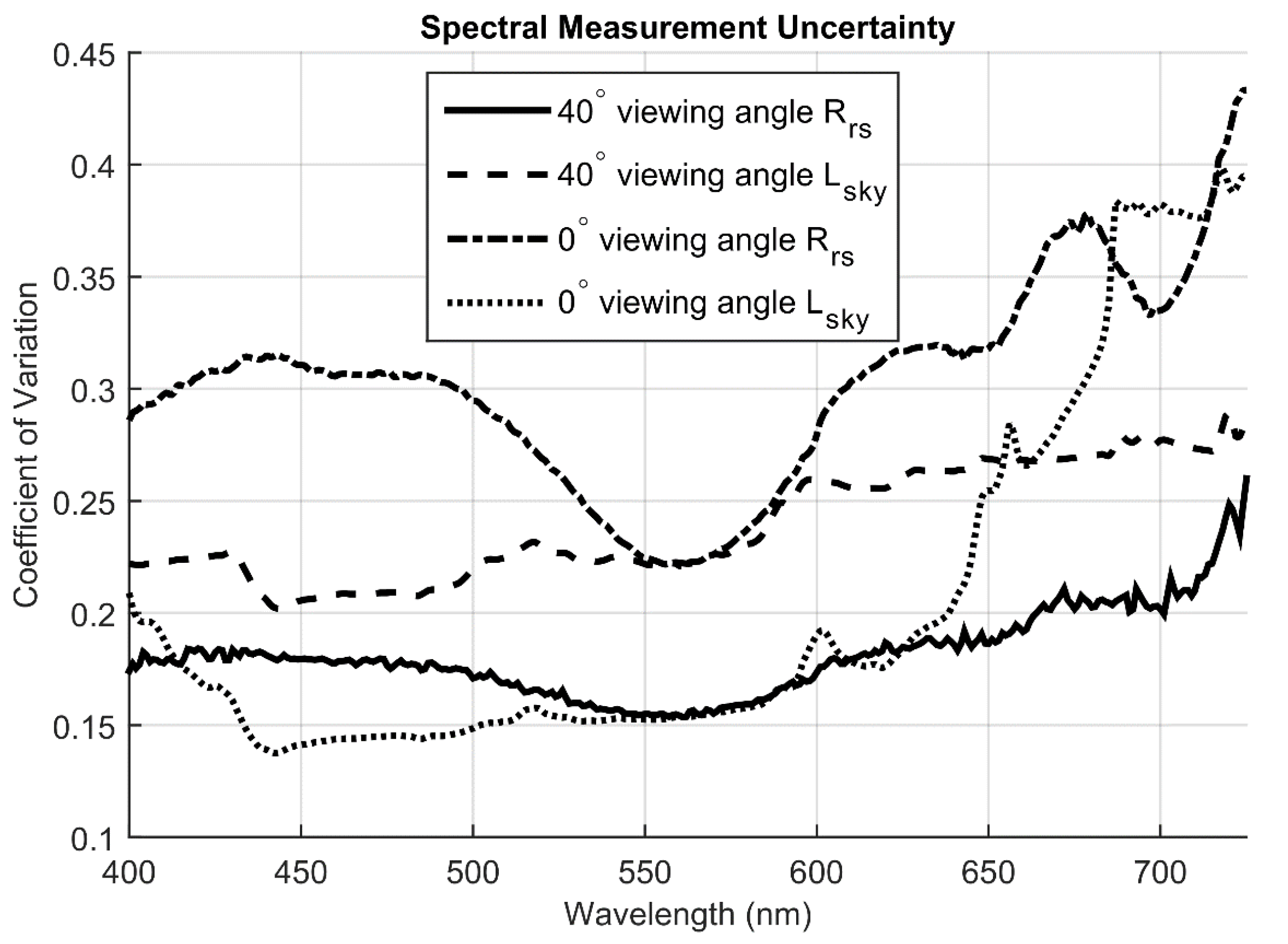
4.6.3. Error from Field Spectrometer Measurements

4.6.4. Error from constituent quantification and laboratory methods
5. Conclusions
Acknowledgments
Author Contributions
Conflicts of Interest
References
- IOCCG. Why Ocean Colour? The Societal Benefits of Ocean-Colour Technology; Reports of the International Ocean-Colour Coordinating Group, Platt, T., Hoepffner, N., Stuart, V., Brown, C., Eds.; IOCCG: Dartmouth, NS, Canada, 2008. [Google Scholar]
- Kuchinke, C.P.; Gordon, H.R.; Franz, B.A. Spectral optimization for constituent retrieval in Case 2 waters II: Validation study in the Chesapeake Bay. Remote Sens. Environ. 2009, 113, 610–621. [Google Scholar]
- Santini, F.; Alberotanza, L.; Cavalli, R.M.; Pignatti, S. A two-step optimization procedure for assessing water constituent concentrations by hyperspectral remote sensing techniques: An application of the highly turbid Venice lagoon waters. Remote Sens. Environ. 2010, 114, 887–898. [Google Scholar] [CrossRef]
- Dong, J.; Xiao, X.; Sheldon, S.; Biradar, C.; Duong, N.D.; Hazarika, M. A comparison of forest cover maps in Mainland Southeast Asia from multiple sources: PALSAR, MERIS, MODI and FRA. Remote Sens. Environ. 2012, 127, 60–73. [Google Scholar] [CrossRef]
- Hommersom, A.; Kratzer, S.; Laanen, M.; Ansko, I.; Ligi, M.; Bresciani, M.; Giardino, C.; Beltran-Abaunza, J.M.; Moore, G.; Wernand, M.; et al. Intercomparison in the field between new WISP-3 and other radiometers (TriOS Ramses, ASD FieldSpec, and TACCS). J. Appl. Remote Sens. 2013, 6, 063615. [Google Scholar] [CrossRef]
- Torrecilla, E.; Stramski, D.; Reynolds, R.A.; Millan-Nunez, E.; Piera, J. Cluster analysis of hyperspectral optical data for discriminating phytoplankton pigment assemblages in the open ocean. Remote Sens. Environ. 2011, 115, 2578–2593. [Google Scholar] [CrossRef] [Green Version]
- Bresciani, M.; Rossini, M.; Morabito, G.; Matta, E.; Pinardi, M.; Cogliati, S.; Julitta, T.; Colombo, R.; Braga, F.; Giardino, C. Analysis of within- and between-day chlorophyll-a dynamics in Mantua Superior Lake, with a continuous spectroradiometric measurement. Mar. Freshw. Res. 2013, 64, 303–316. [Google Scholar] [CrossRef]
- Oubelkheir, K.; Clementson, L.A.; Webster, I.T.; Ford, P.W.; Dekker, A.G.; Radke, L.C.; Daniel, P. Using inherent optical properties to investigate biogeochemical dynamics in a tropical macrotidal coastal system. J. Geophys. Res. 2006, 111, C0702. [Google Scholar] [CrossRef]
- Lee, Z.; Du, K.; Voss, K.J.; Zibordi, G.; Lubac, B.; Arnorne, R.; Weidemann, A. An inherent-optical-property-centered approach to correct the angular effects in water-leaving radiance. Appl. Opt. 2011, 50, 3155–3167. [Google Scholar] [CrossRef] [PubMed]
- Simis, S.G.H.; Olsson, J. Unattended processing of shipborne hyperspectral reflectance measurements. Remote Sens. Environ. 2013, 135, 202–212. [Google Scholar] [CrossRef]
- Gons, H.J. Optical teledetection of chlorophyll a in turbid inland waters. Environ. Sci. Technol. 1999, 33, 1127–1132. [Google Scholar] [CrossRef]
- Lee, Z.; Carder, K.L.; Mobley, C.D.; Steward, R.G.; Patch, J.S. Hyperspectral remote sensing for shallow waters: I. A semianalytical model. Appl. Opt. 1998, 37, 6329–6338. [Google Scholar] [CrossRef] [PubMed]
- Lee, Z.; Carder, K.L.; Mobley, C.D.; Steward, R.G.; Patch, J.S. Hyperspectral remote sensing for shallow waters: 2. Deriving bottom depths and water properties by optimization. Appl. Opt. 1999, 38, 3831–3843. [Google Scholar] [CrossRef] [PubMed]
- Mobley, C.D. Estimation of the remote-sensing reflectance from above-surface measurements. Appl. Opt. 1999, 38, 7442–7455. [Google Scholar] [CrossRef] [PubMed]
- De Haan, J.F.; Kokke, J.M.M. Remote Sensing Algorithm Development Toolkit I: Operationalization of Atmospheric Correction Methods for Tidal and Inland Waters; Netherlands Remote Sensing Board: Delft, The Netherlands, 1996. [Google Scholar]
- Ruddick, K.G.; de Cauwer, V.; Park, Y.J.; Moore, G. Seaborne measurements of near infrared water-leaving reflectance: The similarity spectrum for turbid waters. Limnol. Oceanogr. 2006, 51, 1167–1179. [Google Scholar] [CrossRef]
- Mobley, C.D. Light and Water: Radiative Transfer in Natural Waters; Academic Press, Inc.: London, UK, 1994. [Google Scholar]
- Hakvoort, H.; de Haan, J.; Jordans, R.; Vos, R.; Peters, S.; Rijkeboer, M. Towards operational airborne remote sensing of water quality in The Netherlands. Int. Arch. Photogramm. Remote Sens. 2000, 33, 489–495. [Google Scholar]
- Brando, V.E.; Anstee, J.M.; Wettle, M.; Dekker, A.G.; Phinn, S.R.; Roelfsema, C. A physics based retrieval and quality assessment of bathymetry from suboptimal hyperspectral data. Remote Sens. Environ. 2009, 113, 755–770. [Google Scholar] [CrossRef]
- Morel, A.; Voss, K.J.; Gentili, B. Bidirectional reflectance of oceanic waters: A comparison of modeled and measured upward radiance fields. J. Geophys. Res. 1995, 100, 13143–13150. [Google Scholar] [CrossRef]
- Gordon, H.R.; Brown, O.B.; Evans, R.H.; Brown, J.W.; Smith, R.C.; Baker, K.S.; Clark, D.K. A semianalytic radiance model of ocean color. J. Geophys. Res. 1988, 93, 10909–10924. [Google Scholar] [CrossRef]
- Lee, Z.; Carder, K.L.; Arnorne, R.A. Deriving inherent optical properties from water color: A multiband quasi-analytical algorithm for optically deep waters. Appl. Opt. 2002, 41, 5755–5772. [Google Scholar] [CrossRef] [PubMed]
- Garver, S.A.; Siegel, D.A. Inherent optical property inversion of ocean color spectra and its biogeochemical interpretation 1: Time series from the Sargasso Sea. J. Geophys. Res. 1997, 102, 18607–18625. [Google Scholar] [CrossRef]
- Maritorena, S.; Siegel, D.A.; Peterson, A.R. Optimization of a semi-analytical ocean color model for global-scale applications. Appl. Opt. 2002, 41, 2705–2714. [Google Scholar] [CrossRef] [PubMed]
- Giardino, C.; Candiani, G.; Bresciani, M.; Lee, Z.P.; Gagliano, S.; Pepe, M. BOMBER: A tool for estimating water quality and bottom properties from remote sensing images. Comput. Geosci. 2012, 45, 313–318. [Google Scholar] [CrossRef]
- Huang, S.; Li, Y.; Shang, S.; Shang, S. Impacts of computational methods and spectral models on the retrieval of optical properties via spectral optimization. Opt. Express 2013, 21, 6257–6273. [Google Scholar] [PubMed]
- Cannizzaro, J.P.; Carder, K.L. Estimating chlorophyll a concentrations from remote-sensing reflectance in optically shallow waters. Remote Sens. Environ. 2006, 101, 13–24. [Google Scholar] [CrossRef]
- Smith, R.C.; Baker, K.S. Optical properties of the clearest natural waters (200–800 nm). Appl. Opt. 1981, 20, 177–184. [Google Scholar] [CrossRef] [PubMed]
- Pope, R.M.; Fry, E.S. Absorption spectrum (380–700 nm) of pure water. II. Integrating cavity measurements. Appl. Opt. 1997, 36, 8710–8723. [Google Scholar] [CrossRef] [PubMed]
- Buiteveld, H.; Hakvoort, J.H.M.; Donze, M. The optical properties of pure water. Proc. SPIE 1994, 2258, 174–183. [Google Scholar]
- Chang, C.H.; Liu, C.C.; Wen, C.G. Integrating semianalytical and genetic algorithms to retrieve the constituents of water bodies from remote sensing of ocean color. Opt. Express 2007, 15, 252–265. [Google Scholar] [CrossRef] [PubMed]
- Giardino, C.; Brando, V.E.; Dekker, A.G.; Strombeck, N.; Candiani, G. Assessment of water quality in Lake Garda (Italy) using Hyperion. Remote Sens. Environ. 2007, 109, 183–195. [Google Scholar] [CrossRef]
- Moisan, T.A.H.; Moisan, J.R.; Linkswiler, M.A.; Steinhardt, R.A. Algorithm development for predicting biodiversity based on phytoplankton absorption. Cont. Shelf Res. 2013, 55, 17–28. [Google Scholar] [CrossRef]
- Jerlov, N.G. Optical Oceanography; Elsevier: New York, NY, USA, 1976. [Google Scholar]
- Brando, V.E.; Dekker, A.G. Satellite hyperspectral remote sensing for estuarine and coastal water quality. IEEE Trans. Geosci. Remote Sens. 2003, 41, 1378–1387. [Google Scholar] [CrossRef]
- Van der Woerd, H.J.; Pasterkamp, R. HYDROPT: A fast and flexible method to retrieve chlorophyll-a from multispectral satellite observations of optically complex coastal waters. Remote Sens. Environ. 2008, 112, 1795–1807. [Google Scholar] [CrossRef]
- Hedley, J.; Roelfsema, C.; Phinn, S.R. Efficient radiative transfer model inversion for remote sensing applications. Remote Sens. Environ. 2009, 113, 2527–2532. [Google Scholar] [CrossRef]
- Kruse, F.A.; Lefkoff, A.B.; Boardman, J.W.; Heidebrecht, K.B.; Shapiro, A.T.; Barloon, P.J.; Goetz, A.F.H. The spectral image processing system (SIPS)—Interactive visualization and analysis of imaging spectrometer data. Remote Sens. Environ. 1993, 44, 145–163. [Google Scholar] [CrossRef]
- De Carvalho, O., Jr.; Guimaraes, R.; Gomes, R.; de Carvalho, A.; da Silva, N.; Martins, E. Spectral multiple correlation mapper. In Proceedings of the IEEE International Conference on Geosciences and Remote Sensing Symposium, Denver, CO, USA, 31 July–4 August 2006.
- Low, E.W.; Clews, E.; Todd, P.A.; Tai, Y.C.; Ng, P.K.L. Top-down control of phytoplankton by zooplankton in tropical reservoirs in Singapore? Raffles Bull. Zool. 2010, 58, 311–322. [Google Scholar]
- Clews, E.; Low, E.W.; Belle, C.C.; Todd, P.A.; Eikaas, H.S.; Ng, P.K.L. A pilot macroinvertebrate index of water quality of Singapore’s reservoirs. Ecol. Indic. 2014, 38, 90–103. [Google Scholar] [CrossRef]
- Morel, A.; Prieur, L. Analysis of variations in ocean color. Limnol. Oceanogr. 1977, 22, 709–722. [Google Scholar]
- IOCCG. Remote Sensing of Ocean Colour in Coastal, and Other Optically-Complex, Waters; Reports of the International Ocean-Colour Coordinating Group, Sathyendranath, S., Eds.; IOCCG: Dartmouth, NS, Canada, 2000. [Google Scholar]
- Matthews, M.W.; Bernard, S.; Winter, K. Remote sensing of cyanobacteria-dominant algal blooms and water quality parameters in Zeekoevlei, a small hypertrophic lake, using MERIS. Remote Sens. Environ. 2010, 114, 2070–2087. [Google Scholar] [CrossRef]
- Arar, E.J. In Vitro Determination of Chlorophylls a, b, c1 + c2 and Pheopigments in Marine and Freshwater Algae by Visible Spectrophotometry; EPA: Cincinnati, OH, USA, 1997. [Google Scholar]
- America Public Health Assocation (APHA). Standard Methods for the Examination of Water and Wastewater, 21st ed.; American Public Health Association, American Water Works Association, Water Environment Federation Publication: Washington, DC, USA, 2000. [Google Scholar]
- Bricaud, A.; Stramski, D. Spectral absorption coefficients of living phytoplankton and nonalgal biogenous matter: A comparison between the Peru upwelling area and the Sargasso Sea. Limnol. Oceanogr. 1990, 35, 562–582. [Google Scholar] [CrossRef]
- Cleveland, J.S.; Weidemann, A.D. Quantifying absorption by aquatic particles: A multiple scattering correction for glass-fiber filters. Limnol. Oceanogr. 1993, 38, 1321–1327. [Google Scholar] [CrossRef]
- Kishino, M.; Takahashi, M.; Okami, N.; Ichimura, S. Estimation of the spectral Absorption coefficients of phytoplankton in the sea. Bull. Mar. Sci. 1985, 37, 634–642. [Google Scholar]
- Clementson, L.A.; Parslow, J.S.; Turnbull, A.R.; McKenzie, D.C.; Rathbone, C.E. Optical properties of waters in the Australasian sector of the Southern Ocean. J. Geophys. Res. 2001, 106, 31611–31625. [Google Scholar]
- Mathworks. Optimization Toolbox: User's Guide (r2011b); The MathWorks, Inc.: Natick, MA, USA, 2011; Available online: http://www.mathworks.com/help/releases/R2014a/pdf_doc/optim/optim_tb.pdf (accessed on 5 May 2014).
- Fox, J. Applied Regression Analysis and Generalized Linear Models, 2nd ed.; SAGE Publications, Inc.: London, UK, 2008. [Google Scholar]
- Draper, N.R.; Smith, H. Applied Regression Analysis, 3rd ed.; John Wiley & Sons, Inc.: New York, NY, USA, 1998. [Google Scholar]
- Doxaran, D.; Cherukuru, R.C.N.; Lavender, S.J. Estimation of surface reflection effects on upwelling radiance field measurements in turbid waters. J. Opt. A Pure Appl. Opt. 2004, 6, 690–697. [Google Scholar] [CrossRef]
- Ku, H.H. Statistical concepts in metrology. In Precision Measurement and Calibration: Statistical Concepts and Procedures; Ku, H.H., Ed.; Government Printing Office: Washington, DC, USA, 1969; Volume 1, pp. 296–330. [Google Scholar]
© 2015 by the authors; licensee MDPI, Basel, Switzerland. This article is an open access article distributed under the terms and conditions of the Creative Commons by Attribution (CC-BY) license (http://creativecommons.org/licenses/by/4.0/).
Share and Cite
Bramante, J.F.; Sin, T.M. Optimization of a Semi-Analytical Algorithm for Multi-Temporal Water Quality Monitoring in Inland Waters with Wide Natural Variability. Remote Sens. 2015, 7, 16623-16646. https://doi.org/10.3390/rs71215845
Bramante JF, Sin TM. Optimization of a Semi-Analytical Algorithm for Multi-Temporal Water Quality Monitoring in Inland Waters with Wide Natural Variability. Remote Sensing. 2015; 7(12):16623-16646. https://doi.org/10.3390/rs71215845
Chicago/Turabian StyleBramante, James F., and Tsai Min Sin. 2015. "Optimization of a Semi-Analytical Algorithm for Multi-Temporal Water Quality Monitoring in Inland Waters with Wide Natural Variability" Remote Sensing 7, no. 12: 16623-16646. https://doi.org/10.3390/rs71215845