Development and Evaluation of a Multi-Year Fractional Surface Water Data Set Derived from Active/Passive Microwave Remote Sensing Data

Abstract

The sensitivity of Earth’s wetlands to observed shifts in global precipitation and temperature patterns and their ability to produce large quantities of methane gas are key global change questions. We present a microwave satellite-based approach for mapping fractional surface water (FW) globally at 25-km resolution. The approach employs a land cover-supported, atmospherically-corrected dynamic mixture model applied to 20+ years (1992–2013) of combined, daily, passive/active microwave remote sensing data. The resulting product, known as Surface WAter Microwave Product Series (SWAMPS), shows strong microwave sensitivity to sub-grid scale open water and inundated wetlands comprising open plant canopies. SWAMPS’ FW compares favorably (R² = 91%–94%) with higher-resolution, global-scale maps of open water from MODIS and SRTM-MOD44W. Correspondence of SWAMPS with open water and wetland products from satellite SAR in Alaska and the Amazon deteriorates when exposed wetlands or inundated forests captured by the SAR products were added to the open water fraction reflecting SWAMPS’ inability to detect water underneath the soil surface or beneath closed forest canopies. Except for a brief period of drying during the first 4 years of observation, the inundation extent for the global domain excluding the coast was largely stable. Regionally, inundation in North America is advancing while inundation is on the retreat in Tropical Africa and North Eurasia. SWAMPS provides a consistent and long-term global record of daily FW dynamics, with documented accuracies suitable for hydrologic assessment and global change-related investigations.

1. Introduction

The sensitivity of Earth’s natural wetlands to changes in precipitation and temperature patterns and their role as a significant source of atmospheric methane (CH₄)—an important greenhouse gas—are key climate change questions [1]. Unlike weather station data, from which global precipitation and temperature trends can be inferred, global CH₄ emissions are typically estimated via process-based models calibrated to individual wetland sites [2,3,4,5,6]. In this approach, CH₄ emissions from wetland sites are extrapolated via spatially explicit maps of global wetland distribution, combining static and more recently dynamic inundation maps with hydrological and biogeochemical process features thought to be relevant for methanogenesis [7,8,9,10,11,12,13,14,15,16,17,18,19]. Top-down approaches, such as estimation of atmospheric CH₄ using satellite measurements and inverse models [20,21,22,23] are useful tools in constraining ground-based emission inventories, particularly over tropical wetlands which exhibit higher CH₄ emissions than those estimated from forward calculations [24,25,26]. This emission discrepancy between model approaches may be explained by both a lack of field data available from tropical wetlands and an incomplete representation of the hydrodynamics of shallow tropical wetland complexes [27]. Development and application of spatially comprehensive and temporally consistent maps of global inundation dynamics as model inputs or optimization targets in global methane models are thus crucial for improving our understanding of the role of wetland emissions in the climate system [16].

Several different remote sensing-based approaches haven been taken towards regional to global-scale satellite monitoring of inundation: passive microwave, active microwave and hybrid approaches. Coarse-resolution (25-km) passive and active microwave (MW) data from satellite instruments (e.g., Advanced Microwave Scanning Radiometer-EOS (AMSR-E), SeaWinds-on-QuikSCAT) are well suited for the global monitoring of inundation patterns because they are sensitive to the distribution of liquid water in the landscape and cover large areas with daily repeat periods at high latitudes. Because MW instruments can operate day and night and are not limited by cloud cover, they provide the unique capability for acquiring temporally consistent and continuous records of inundation dynamics, supporting accurate inference of surface water dynamics and related fresh water storage changes. Differences observed between vertically and horizontally polarized brightness temperatures (T_b) by passive MW instruments have long been shown to be effective in measuring large-scale inundation patterns across densely vegetated landscapes [28,29,30,31,32,33,34,35,36]. Common to this approach is the assumption that, across densely vegetated forests, changes in soil moisture and vegetation biomass and structure and associated variations in emissivity caused by both are negligible relative to the influence of inundation.

Radar backscatter (σ⁰) from active MW instruments is also sensitive to inundation conditions and has been used regionally to delineate floods and monitor inundation extent [37,38,39,40,41]. Its higher sensitivity to vegetation structure, relative to T_b, provides a unique capability to characterize biomass variations associated with seasonal plant dynamics [42,43,44,45,46,47,48]. As most major global wetland complexes consist of inundated surfaces that are often vegetated, methods that combine σ⁰ and T_b provided by coarse-resolution active and passive MW instruments would be ideal for the characterization of surface water dynamics in vegetated ecosystems subject to seasonal plant dynamics.

Hybrid approaches combine the strengths of different types of sensors. For example, high-resolution low repeat cycle data can be combined with low-resolution high repeat data to construct an inundation product that provides both high resolution and frequent observation [49,50]. The Global Inundation Extent from Multiple-Satellites (GIEMS) product merges coarse-resolution passive and active MW sensors with optical remote sensing data for mapping inundation globally regardless of the environment [51,52,53,54]. GIEMS corresponds with Synthetic Aperture Radar (SAR) maps of inundation extent in the Amazon basin [53] and has been subsequently employed in estimating surface water storage variations in large river basins [55,56,57]. Jones et al. [58] determine the global surface water extent synergistically leveraging multiple frequencies from a single dual-polarized passive MW instrument [59]. Because long records are crucial for assessing CH₄ model sensitivities to climate change [19], inundation products from satellites of limited lifespan [54,58] will therefore have limited applicability.

Despite its strength, GIEMS has displayed some limitations. First, comparisons with the International Geosphere-Biosphere Programme (IGBP) based MODIS classification of permanent open water over central Russia and western Canada showed that GIEMS missed many small water features (i.e., fractional inundation <10%) in densely forested regions whereas in other regions including the Amazon Basin there was a tendency for GIEMS to overestimate higher inundation fractions [53]. Second, comparisons with SAR-based classifications of inundation in the West Siberian Lowland (WSL) suggested that GIEMS underestimated (overestimated) inundation in forested (non-forested) areas [16]. Third, in the WSL, Bohn et al. [19] showed large discrepancies between inundation from GIEMS and the active/passive MW product of Schroeder et al. [60]. Possible explanations for the mismatch between the two inundation products could be GIEMS’ large radiometer footprint and the retrieval algorithm involving the use of optical satellite data [51,53,54]. Finally, the use of the C-band European Remote Sensing (ERS) scatterometer in the estimation of surface water fractions and the prospect of introducing a record discontinuity using the shorter wavelength K_u-band QuikSCAT (QSCAT) as a substitute for the C-band ERS currently limits GIEMS’ time series from 1993 to 2000, although efforts have been made to GIEMS’ extension using monthly climatologies of the ERS and AVHRR [54]. Given the uncertainty regarding the validity of GIEMS’ surface water fractions, the omission of small water bodies and GIEMS’ relatively short time series, we have developed an alternative long-term record of coarse-resolution fractional open water (FW) and inundated wetlands covering 20+ years (1992–2013).

The primary goal of this study was to develop an alternative FW product with retrieval enhancements in at least three areas with respect to GIEMS. These areas were: (1) accurate and spatially consistent FW; (2) improved low-range FW sensitivity; and (3) extension of the FW time series beyond the C-band ERS record. We asked whether the inclusion of the K_u-band QSCAT, as a means to extend the time series beyond that of the C-band ERS, will lead to a discontinuity in the data record. To accomplish these tasks, we combined the data streams from the Special Sensor Microwave Imager (SSM/I), Special Sensor Microwave Imager/Sounder (SSMI/S)—the passive MW instruments—with those from the ERS, QSCAT and the Advanced Scatterometer (ASCAT)—the active MW instruments—which together cover 20+ years of continuous, global-scale and daily MW observations. The resulting FW retrievals represent 25-km equal area grid cell fractions of open water. We define FW to be inclusive of all water bodies that are unmasked by vegetation. The passive MW sensors provide upwelling T_b at ≥19 GHz which limits penetration of overlying vegetation and litter layers [59,61,62,63]. The FW signal therefore originates from the water surface within open areas and under low density vegetation [64].

We developed a stratified, fully dynamic and calibrated mixture model to aid in the detection and quantification of FW. We evaluated both spatial and temporal accuracy of FW, including seasonal and interannual variability. We examined the 20+ year FW trend and determined the sensitivity of the trend to snow cover screenings. We identified the dominant sources of retrieval error and the land cover conditions that may have caused them. We determined the fundamental physical limitations to FW detection and provided the user with a qualitative map of expected FW accuracy. Finally, we made recommendations as to which satellite observations and data products might be helpful to improve upon the accuracy and sensitivity of our approach. The resulting dataset provides an accurate, consistent and comprehensive global-scale, multi-year data set of daily FW and is suitable for hydrological assessment and global change-related monitoring of FW. This data record together with supporting documentation known as Surface WAter Microwave Product Series (SWAMPS) is to be archived and maintained at the Alaska Satellite Facility Distributed Active Archive Center (ASF DAAC) and available to the world-wide science community.

2. Data Processing and Analysis

2.1. Passive and Active Microwave Satellite Data Record Construction

T_b from SSM/I and SSMI/S and σ⁰ from ERS [65], QSCAT [66] and ASCAT [67] were chosen to support the generation of SWAMPS over a 20+ year study period (1992–2013). We used the multi-frequency, dual-polarized SSM/I and SSMI/S Level-3 T_b observations from the National Snow & Ice Data Center [68], binned as global and northern hemisphere Equal-Area Scalable Earth (EASE) grids at 25-km spatial resolution [69]. The gridding procedures for these data follow the methods described in Armstrong et al. 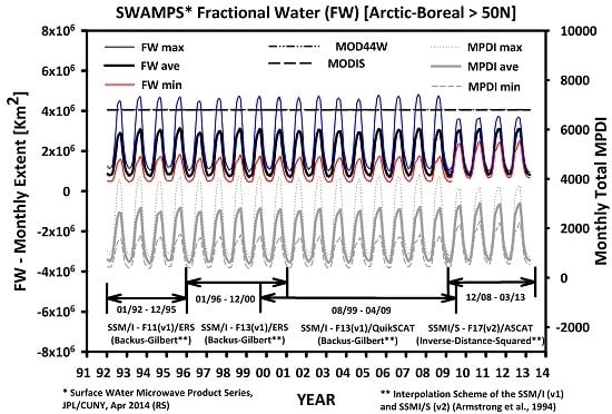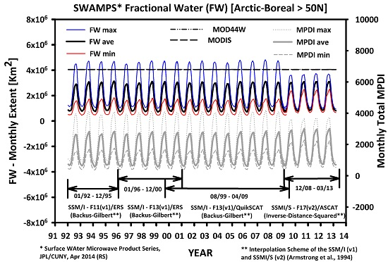[68] and include the Backus-Gilbert (v1) and Inverse-Distance-Squared (v2) interpolation for respective SSM/I and SSMI/S instrument periods. Observations which use v1-gridding began in 1987 and ended in 2009; v2 covered the remainder of the study period including a 2+ year overlap period with v1.

Overlap was utilized to reduce T_b cross-sensor differences [68]. To do so, we constructed linear models from two years of overlapping, high-quality v1 and v2 records, separately for each frequency, polarization and overpass, appropriate to each platform, following previously developed methods [70]. High-quality T_b records were obtained from grid cells at least two cells away from the nearest water body and dominated (>80%) by a single forest cover as defined by the high-resolution (1-km) MODIS IGBP [71] land cover (LC) product (MODIS LC) binned previously to the EASE-grids [72]. v1 and v2 records that were more than 30 min apart or covered tropical forest were excluded. This approach allowed for maximizing T_b seasonal variability while minimizing T_b differences resulting from differences in acquisition time and method of interpolation.

T_b observations over land are largely influenced by surface temperature variations [59,62,70]. To support the derivation of FW, this study employed the Microwave Polarization Difference Index (MPDI) from the 19 GHz band, defined as:

$$MPDI=(T_{b(V)}-T_{b(H)})/(0.5(T_{b(V)}+T_{b(H)}))$$

(1)

where T_b(v) and T_b(h) are the brightness temperatures at respective vertical (v) and horizontal (h) polarization. We employed only morning overpasses, to capture surface conditions as close to isothermal as practical. Partitioning of the polarization difference over its sum is useful because it cancels out the surface temperature component of T_b, leaving a quantity that is largely dependent on the contributions from open water and vegetation [61,73]. Generally, the MPDI increases with the presence of open water bodies and decreases with increasing vegetation density.

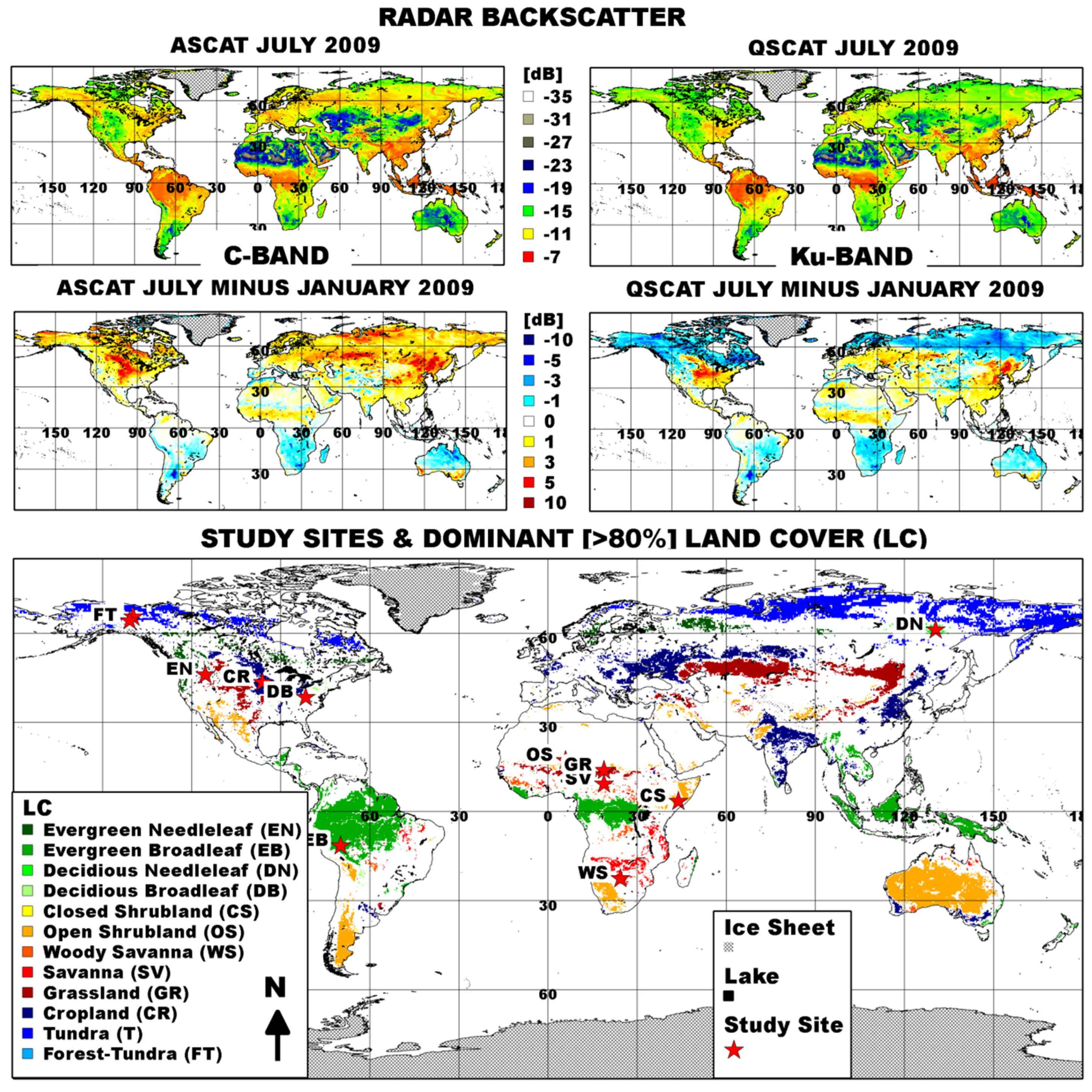
To account for the depolarization effect that vegetation has on total MPDI and to maximize sensor sensitivity to the presence of vegetation structure and biomass dynamics in inundated areas, concurrent, high-quality σ⁰ observations from the ERS, QSCAT and ASCAT were acquired to solve for FW on a daily basis. We employed Level-2, VV-polarized C-band ERS, K_u-band QSCAT and C-band ASCAT and gridded these data to the EASE-grids of the T_b record using drop-in-the-bucket averaging (i.e., samples that fell within a grid cell were averaged together) with no swath averaging. σ⁰ coverage began in 1992 and is ongoing. The ERS and QSCAT records began in 1992 and 1999, and ended in 2000 and 2009, respectively. ASCAT covered the remainder of the study period including 1+ year of overlap with QSCAT.

A fundamental difficulty with utilizing the ERS and ASCAT for the continuous monitoring of inundated vegetation structure and biomass dynamics is additional variability in the signal caused by changes in the angle of incidence [42,43,74,75]. Following from prior results of Long and Hardin [76], a method for deriving the normalized σ⁰ coefficients at a reference incidence angle of 54°, equal to that of the QSCAT, was developed. The method is based on a simple forward model of the form:

$${\mathsf{\sigma }}^0(\mathsf{\theta })=\mathsf{\alpha }+\mathsf{\beta }(\mathsf{\theta }-54°)$$

(2)

where σ⁰(θ) is backscatter acquired at incidence angle θ, α is the incidence angle corrected σ⁰ in dB normalized to 54° and β is a slope factor approximating the change in σ⁰ with incidence angle (θ) in dB/°. We combined a 56-day moving window approach with grid cell-wise linear regression analysis to compute time-averaged, daily α and β values by combining σ⁰ measurements from each swath, overpass and all antennae regardless of look angle for all ASCAT data collected between 11 November 2008 and 31 March 2013. Time-window averaged σ⁰ values were computed for four 10 degree wide incidence angle bins and aggregated to the EASE-grids using drop-in-the-bucket averaging. Since σ⁰ is a measure on a logarithmic scale, it must be anti-logged prior to calculating arithmetic means. The slope factor β for each day was obtained from binned σ⁰ via least-squares linear fits and the resulting slope image from the regression analysis of all grid cells was kept. Likewise, we developed a daily ASCAT climatology of the slope by averaging σ⁰ from all years (2009–2012). The resulting time-averaged slope images were input to equation (2) and the VV-polarized and incidence angle normalized backscatter α at 54° for each day, swath and satellite overpass between 11th November 2008 and 31st March 2013 was computed and aggregated to the EASE-grids using drop-in-the-bucket averaging. Likewise, images of the slope obtained from averaging 4 years of ASCAT data were input to equation (2) and the VV-polarized and incidence angle corrected ERS backscatter α at 54° for each day, swath and overpass between 1st January 1992 and 31st December 2000 was computed and aggregated to the EASE-grids.

A radiometric slope correction was performed prior to the incidence angle correction to reduce the effects of incidence angle and illuminated target area on total σ⁰, following from the approach of Sun et al. [77]. First, for each radar pulse within each EASE-grid cell, we calculated local incidence angle θ relative to slope and aspect provided by the Global Land One-km Base Elevation (GLOBE) Digital Elevation Model (DEM) of Knowles [78] binned previously to the EASE-grids as:

$$\cos (\mathsf{\theta })=\sin ({\mathsf{\alpha }}_{DEM})\sin ({\mathsf{\alpha }}_{SCAT})\cos ({\mathsf{\beta }}_{SCAT}-{\mathsf{\beta }}_{DEM})+\cos ({\mathsf{\alpha }}_{DEM})\cos ({\mathsf{\alpha }}_{SCAT})$$

(3)

where θ is the grid-based incidence angle, ${\alpha }_{DEM}$ is the slope angle provided by GLOBE, ${\alpha }_{SCAT}$ is the incidence angle of the ERS, QSCAT and ASCAT scatterometers (SCAT), ${\beta }_{DEM}$ is the aspect obtained from GLOBE and ${\beta }_{SCAT}$ is the momentary look angle of the SCAT. Second, we corrected σ⁰ by relating the incidence angle of the SCAT to the local incidence angle obtained from GLOBE in Equation (3) by:

$${{\mathsf{\sigma }}^0}_{DEM}={{\mathsf{\sigma }}^0}_{SCAT}\sin (\mathsf{\theta })/\sin ({\mathsf{\alpha }}_{SCAT})$$

(4)

where σ⁰_DEM is the terrain-corrected σ⁰ in dB, σ⁰_SCAT is σ⁰ provided by the SCAT, θ is the incidence angle obtained from Equation (3) and α_SCAT is the local incidence angle of the SCAT.

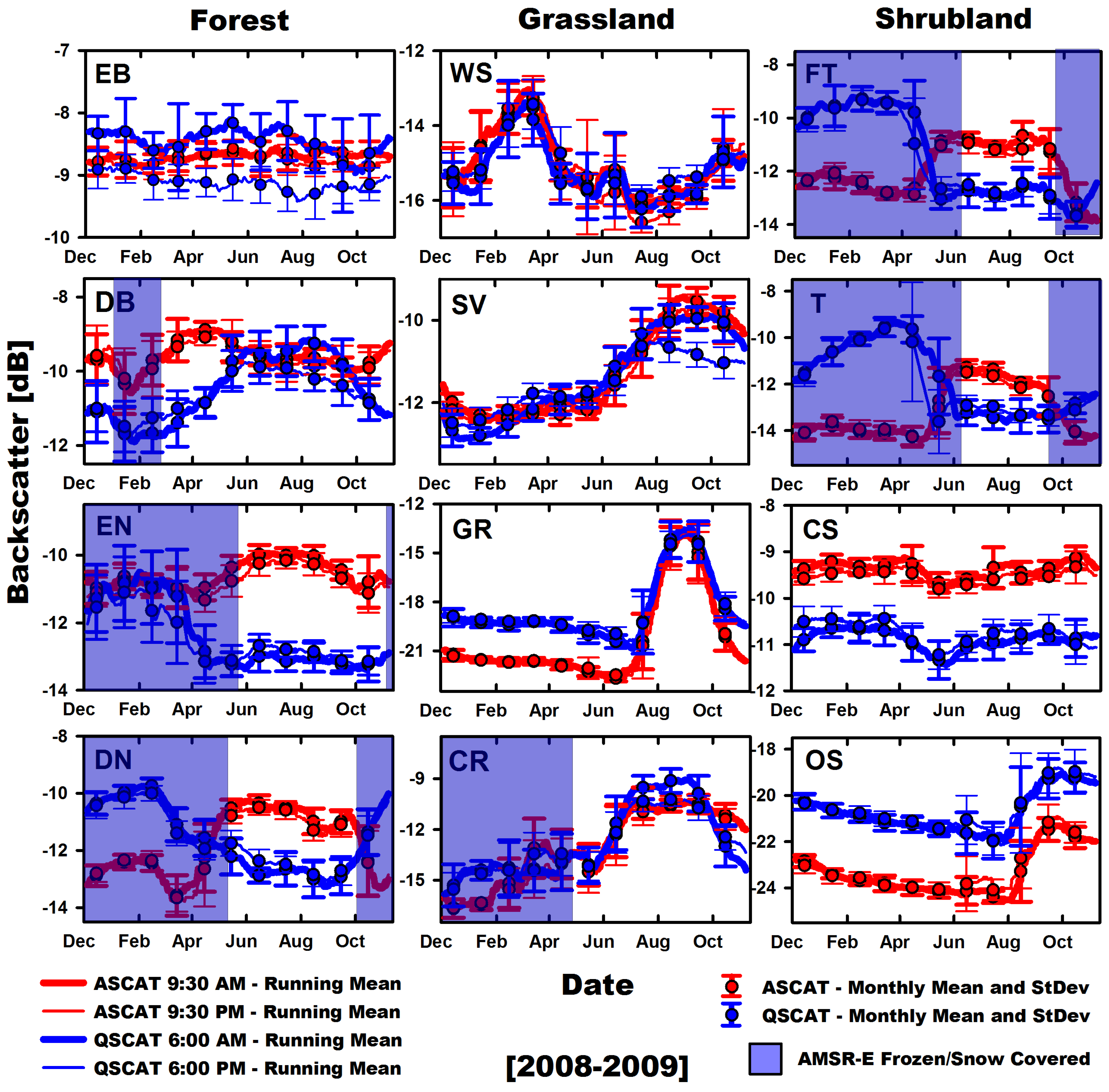
The suitability of the incidence angle and radiometric slope correction for the purpose of extending the FW record beyond the QSCAT period was evaluated next. To do so, we examined the temporal correspondence between the constant incidence angle QSCAT and the incidence angle corrected ASCAT during 1 year of overlap (November 2008–November 2009). We chose 12 vegetated and homogenous (80% classified as a single LC) evaluation sites spanning the range of MODIS LC types. Of these, six sites were identified as having seasonally frozen ground and snow cover conditions, following previously developed screening methods [60]. To reduce the effects of weather, we aggregated daily σ⁰ into 28-day moving composites including monthly means. Metrics of temporal correspondence were reported separately for screened (i.e., seasonal frozen ground and snow cover was removed) and unscreened time series as well as for each satellite overpass to determine the orbit of maximum correspondence. Investigations on the site level were supported by grid cell-wise global calculations of Pearson’s correlation coefficients (R), excluding grid cells with ≥50% water bodies, snow/ice and urban/built-up as identified by the MODIS LC. To aid in the interpretation of spatial R patterns and to assess whether the patterns determined relate to LC and associated canopy structural differences, we stratified R based on grid cells dominated (>80%) by a single MODIS LC.

2.2. Definition of the Global SWAMPS Domains

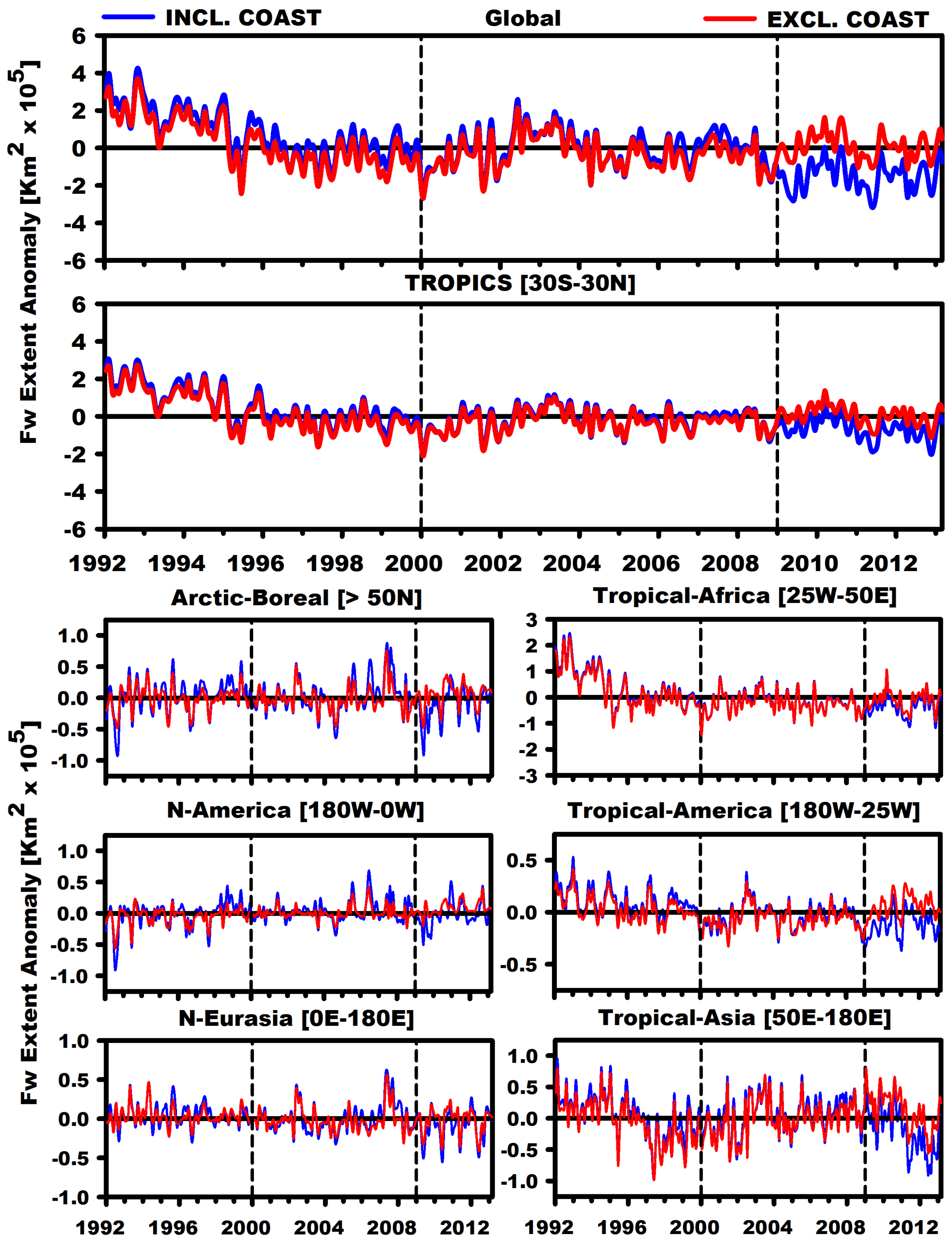
We limited the spatial extent over which SWAMPS provides daily FW to the global land surface with <100% water bodies, snow/ice and urban/built-up as defined by the MODIS LC [72]. This domain includes inland and coastal grid cells with FW contributions from both ocean and inland water bodies. Additionally, we screened this domain for grid cells with ≥50% water bodies to define FW in SWAMPS without costal contributions (i.e., SWAMPS excl. coast). This additional screening eliminates a large proportion of ocean, non-ocean (e.g., large lakes) and coastal water contributions (e.g., large estuaries, river deltas and other coastal wetlands) from the SWAMPS domain and is consistent with the terrestrial focus of the global land parameter database [58]. Seasonal snow cover and precipitating clouds over snow free surfaces can compromise FW. Screening for these conditions is thus crucial for providing accurate FW. We adopted the decision tree of Grody and Basist [79] applied to daily (morning) T_b records to remove grid cells contaminated by snow and frozen ground. Wet snowpacks common during winter warm periods cannot be identified with this approach [80] and thus, if not removed from the domain, introduce erroneously high FW due to being misinterpreted as wide-spread landscape inundation. To account for this effect, we first adopted the method of Chang et al. [81] to estimate daily snow water equivalent (SWE) over grid cells identified by the decision tree, and second applied a 28-day moving window to SWE to conservatively remove previously unidentified grid cells of, e.g., wet, and snow. We employed the decision tree of Ferraro [82] applied to the T_b record to remove grid cells contaminated by precipitating clouds.

2.3. Data Record Development, Approach and Assumptions

Derivation of the SWAMPS product employs a LC-supported dynamic mixture model approach using time series satellite remote sensing radar σ⁰ and radiometric T_b data from a variety of sensors and wavelengths. The approach is to detect landscape inundation by identifying the temporal response of σ⁰ or T_b to changes in the dielectric constant of the land surface that occurs as the soil surface transitions between non-inundated and inundated conditions. The dynamic mixture model approach assumes that the large change in dielectric constant occurring between non-inundated and inundated surface conditions dominates the corresponding σ⁰ and T_b temporal dynamics across the non-frozen seasons, rather than other sources of temporal variability such as changes in canopy structure and biomass, atmospheric moisture variability or large precipitation events. Whether this assumption is valid for most land covers across the global domain will be examined in the results section.

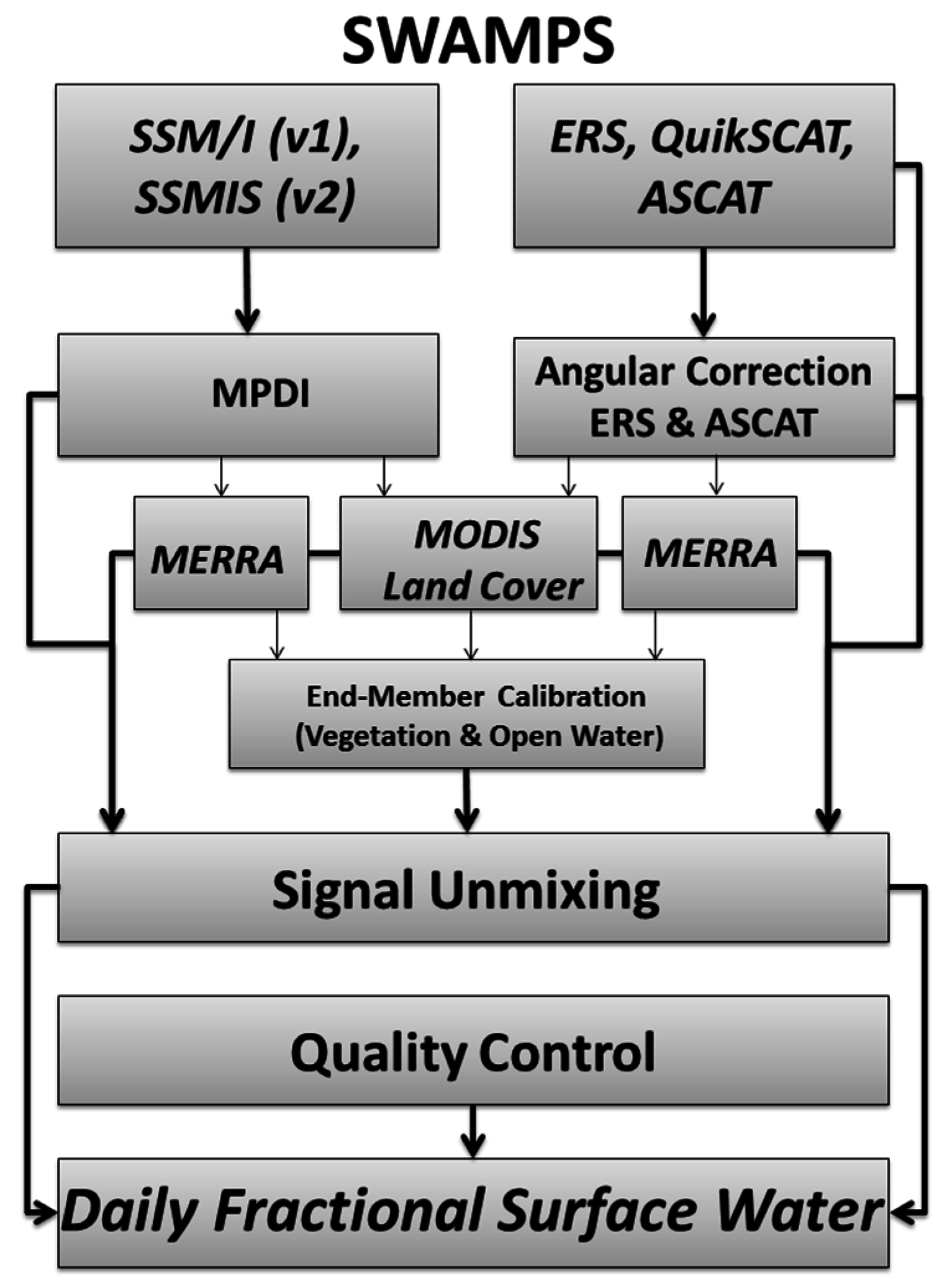
To support the derivation of FW across the limits of our domain, we developed and applied a dynamic mixture model calibrated for FW detection to daily records of passive (MPDI) and active (σ⁰) MW observations (Figure 1). Construction of the mixture model involved a four step process, consisting of (1) development of a set of LC-specific models approximating seasonal biomass dynamics (i.e., the dynamic vegetation end-member); (2) definition of a dynamic open water end-member over land using input from the Modern-Era Retrospective Analysis for Research and Application (MERRA) reanalysis of Rienecker et al. [83]; (3) un-mixing of the FW component given (1) and (2) and (4) construction of a consistent, global record of daily FW dynamics across multiple years.

LC-specific predictive models were developed to aid in quantifying the dynamic vegetation end-member. Input to the derivation of these models was a regression analysis applied separately to data from record periods of concurrent passive (v1 and v2) MPDI and active (ERS, QSCAT and ASCAT) σ⁰ MW observations over grid cells spanning dominant MODIS LC types. MODIS LC provides a total of 17 LC classes [71,72]. Grid cells occupied by less than 50% of a single LC were rejected, including pixels containing any amount of water bodies, permanent wetlands and snow/ice as defined by the MODIS LC. LC classes expected to produce different MW responses when low and high-latitude regions of the same class are compared were split. This included open shrubland, woody savanna, savanna, grassland and barren land. To reduce the impact of weather, monthly climatologies from snow, ice and precipitation-screened MPDI and σ⁰ observations were computed prior to the regression analysis. Monthly climatologies were generated from monthly means which were generated from daily MPDI and σ⁰ observations for each record period. Screening of these data follow the methods outlined in the previous section. We used both linear and non-linear regression models to construct an optimal set of LC-specific model predictions from these data. Model performance was examined and those models which best fit the data were chosen. The resulting regression models approximate, for each LC, sub-class and record period separately, the vegetation end-member for MPDI and σ⁰ regardless of the ratio of land to water within the satellites’ field of views.

Figure 1. Flow chart of the Surface WAter Microwave Product Series (SWAMPS) surface water fraction retrieval scheme including the calibration of vegetation and open water end-members and post-product quality control.

Figure 1. Flow chart of the Surface WAter Microwave Product Series (SWAMPS) surface water fraction retrieval scheme including the calibration of vegetation and open water end-members and post-product quality control.

Open water bodies strongly enhance sensitivity to atmospheric moisture variability when high-frequency (≥19 GHz) T_b observations are used for FW retrieval [84]. σ⁰ of calm water is much lower than over waters roughened by wind or raindrops [85,86]. To solve for FW on a daily grid-by-grid cell basis, an end-member for open water that accounts for the effects of atmospheric variability on MPDI and σ⁰ must be defined prior to FW retrieval. We defined this end-member by constructing regression models derived from empirical relationships between precipitation-screened MPDI and σ⁰ records, and concurrent, hourly inputs of water vapor, cloud liquid water and 2 m wind speed from MERRA over open seas. Using the reanalysis as input, the models developed approximate the open water end-member for MPDI and σ⁰ on land regardless of the ratio of land to water within the satellites’ field of views.

We now are able to combine the results from the regression analysis of vegetation dynamics with those from the end-member calibration of open water to quantify daily FW on a grid-by-grid cell basis within the limits of our domain. We employed a root-finding algorithm that iteratively fits a best linear solution between the open water end-member modeled independently by MERRA, the LC-specific vegetation end-member estimated from monthly MPDI and σ⁰ climatologies, and daily input from the passive and active MW sensors, to obtain LC-specific and atmospherically corrected daily FW relative to end-members fully covered by water and vegetation. To obtain FW within grid cells composed of more than one MODIS LC, LC-specific FW was scaled linearly and summed according to the fractional coverage and number of LC classes within each grid cell provided by MODIS. We applied the following equation to obtain total water fraction FW_tot on a daily grid-by-grid cell basis:

$$F{W}_{tot}=\frac{{\displaystyle \sum _{lc=1}^{N}f{w}_{lc}}fra{c}_{lc}}{fra{c}_{tot}}$$

(5)

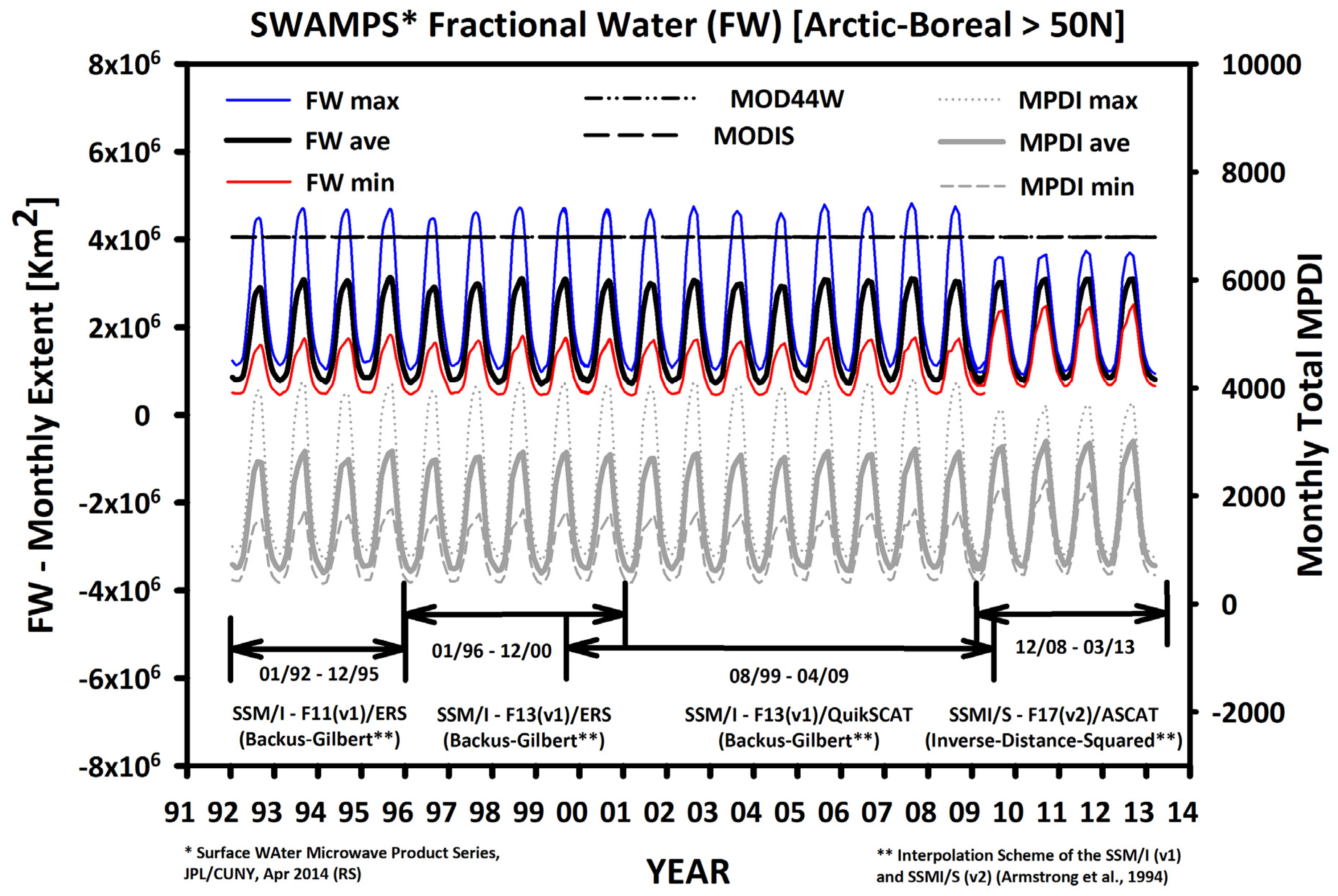
where fw_lc and frac_lc denote LC-specific FW obtained from linear un-mixing, scaled by the LC-specific grid cell fraction and summed over N land cover classes, and frac_tot is the grid-based total LC fraction from MODIS, excluding contributions from water bodies, permanent wetlands and snow/ice as defined by the MODIS LC. The output of Equation (5) is the daily LC-based and atmospherically corrected total surface water fraction FW. At present, SWAMPS is available from 1992 until March 2013 consisting of daily FW record periods herein referred to as v1-ERS (01/1992–12/2000), v1-QSCAT (07/1999–04/2009) and v2-ASCAT (11/2008–03/2013).

2.4. Accuracy Assessment

To facilitate accuracy assessment, the following temporal composites of daily FW were generated first for each record period: (1) monthly mean, minimum and maximum; (2) annual mean and average annual mean generated from (1); (3) monthly climatology generated from monthly means; and (4) the average annual maximum and minimum generated from (3). We then use these records to assess annual and seasonal FW extent and variability within the limits of our domain and the following continental regions: Arctic-Boreal (>50°N)—North America: 180°W–0°W and North Eurasia: 0°E–180°E; Tropics (30°S–30°N)—Tropical America: 180°W–25°W, Tropical Africa: 25°W–50°E and Tropical Asia: 50°E–180°E.

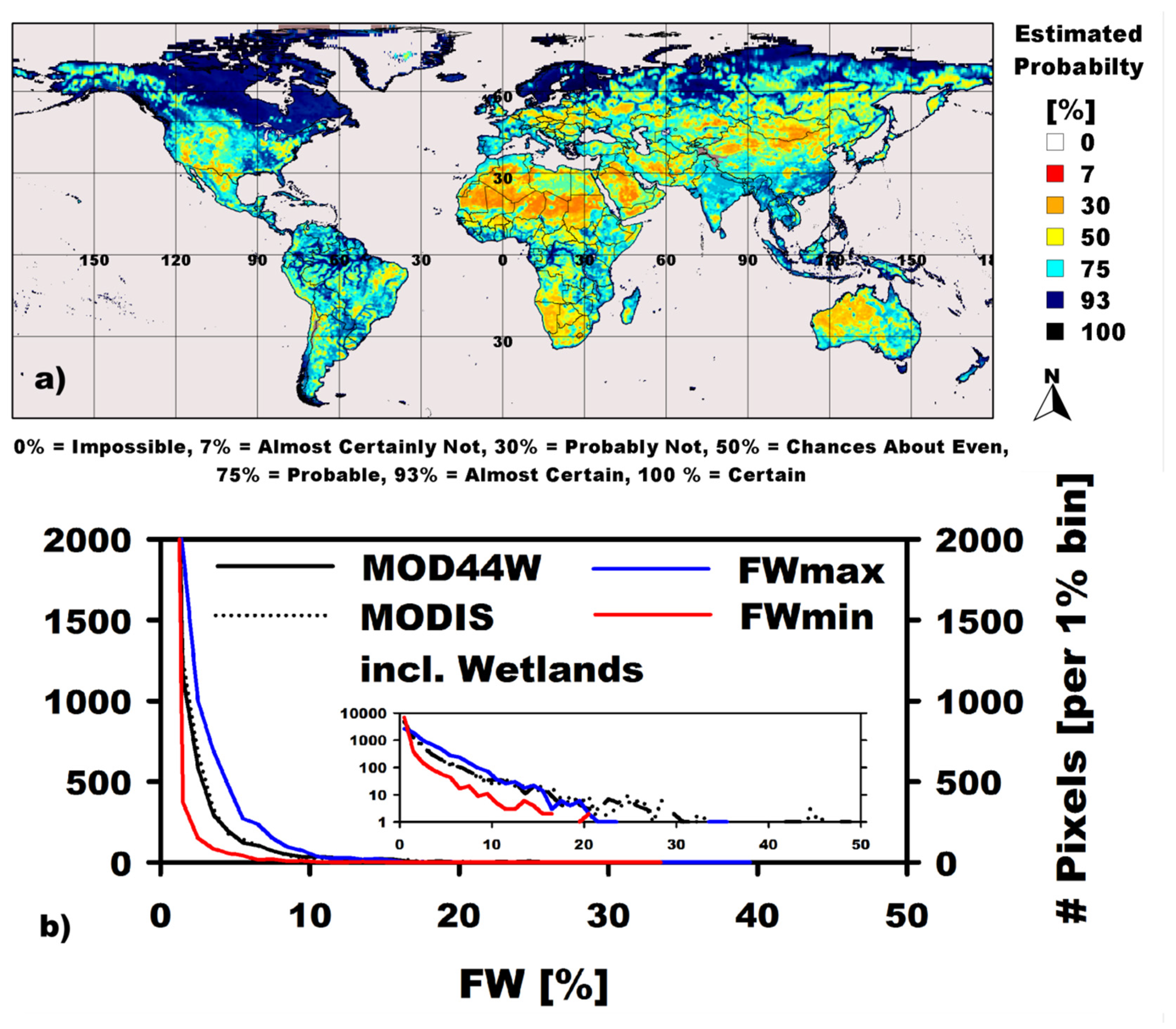
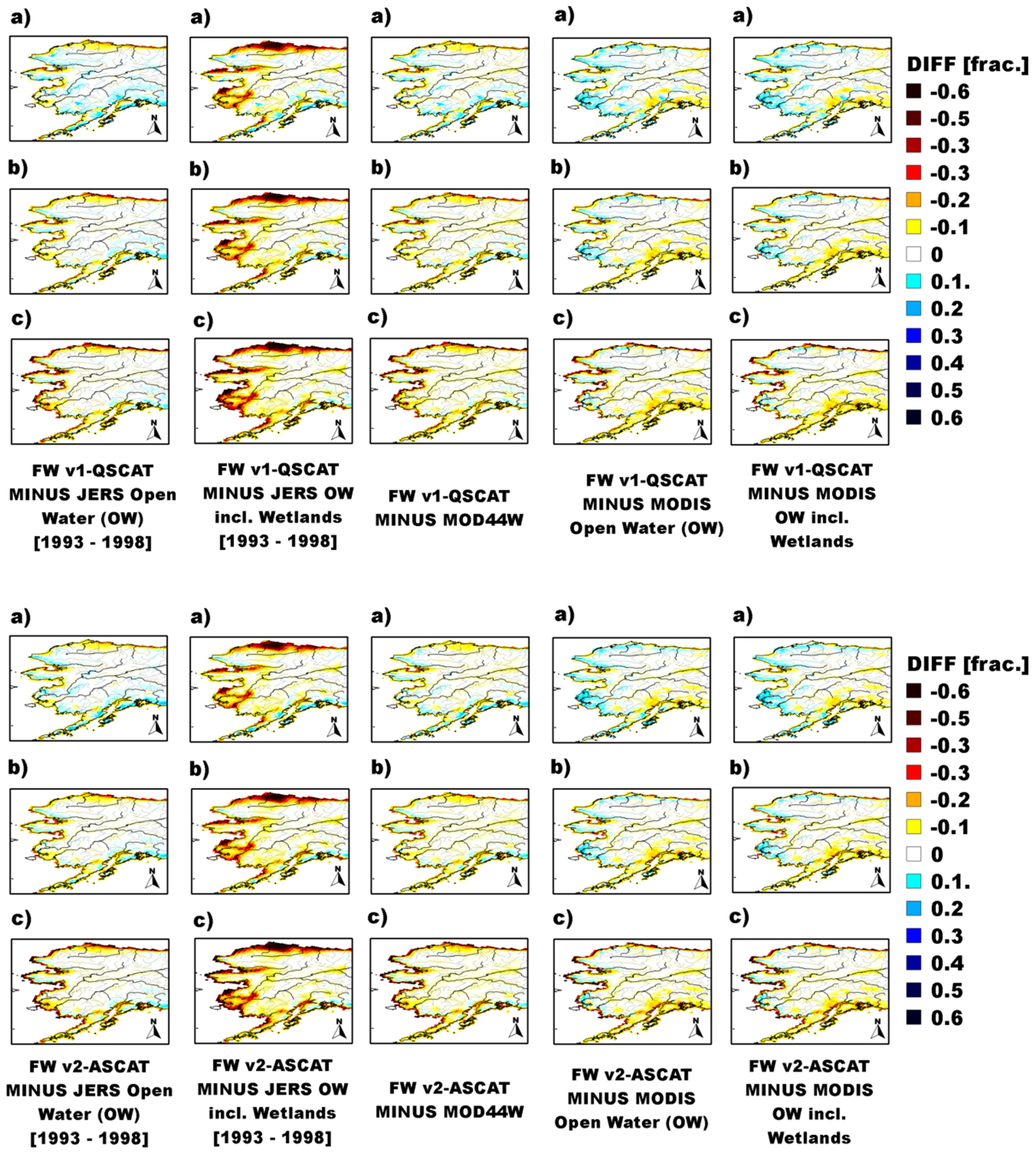
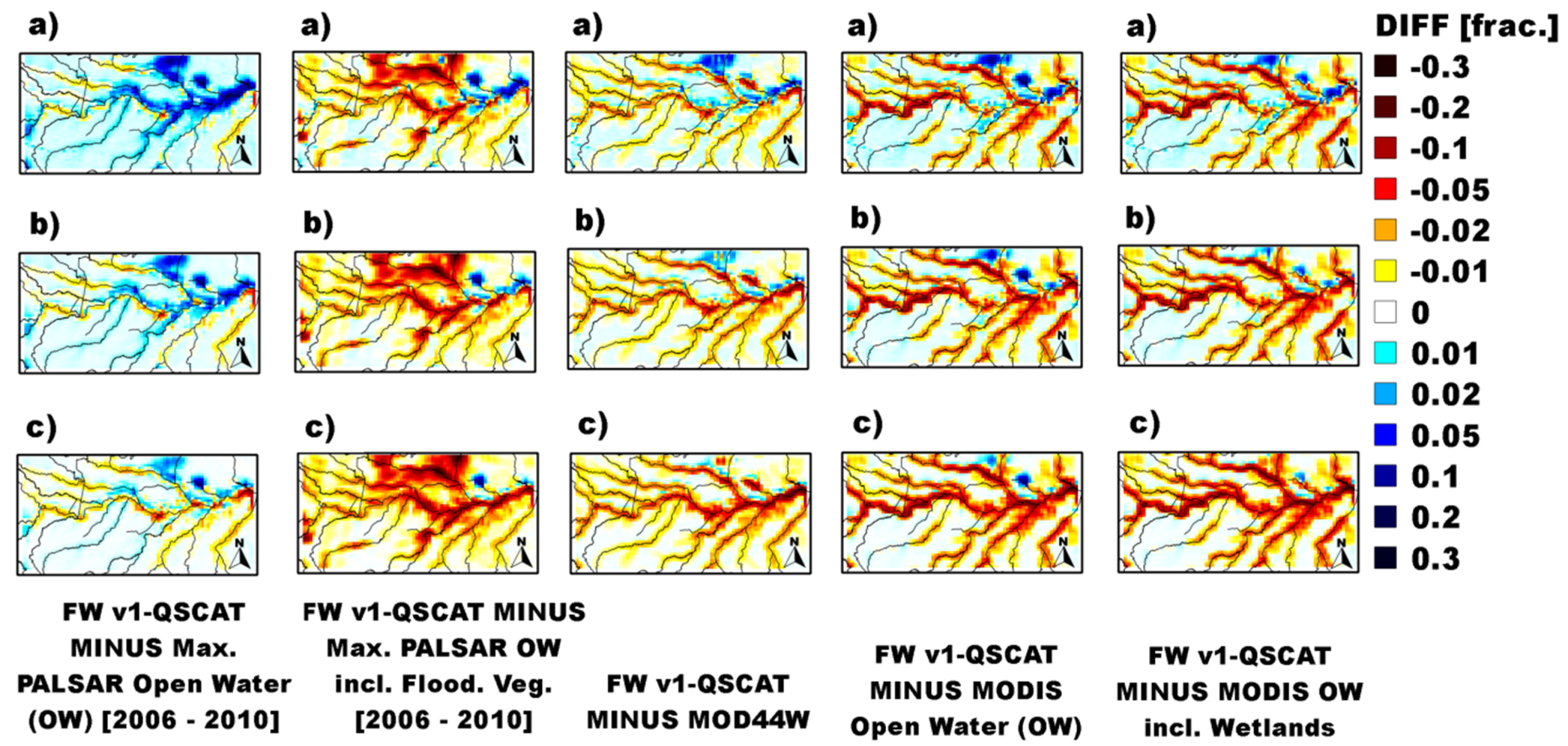
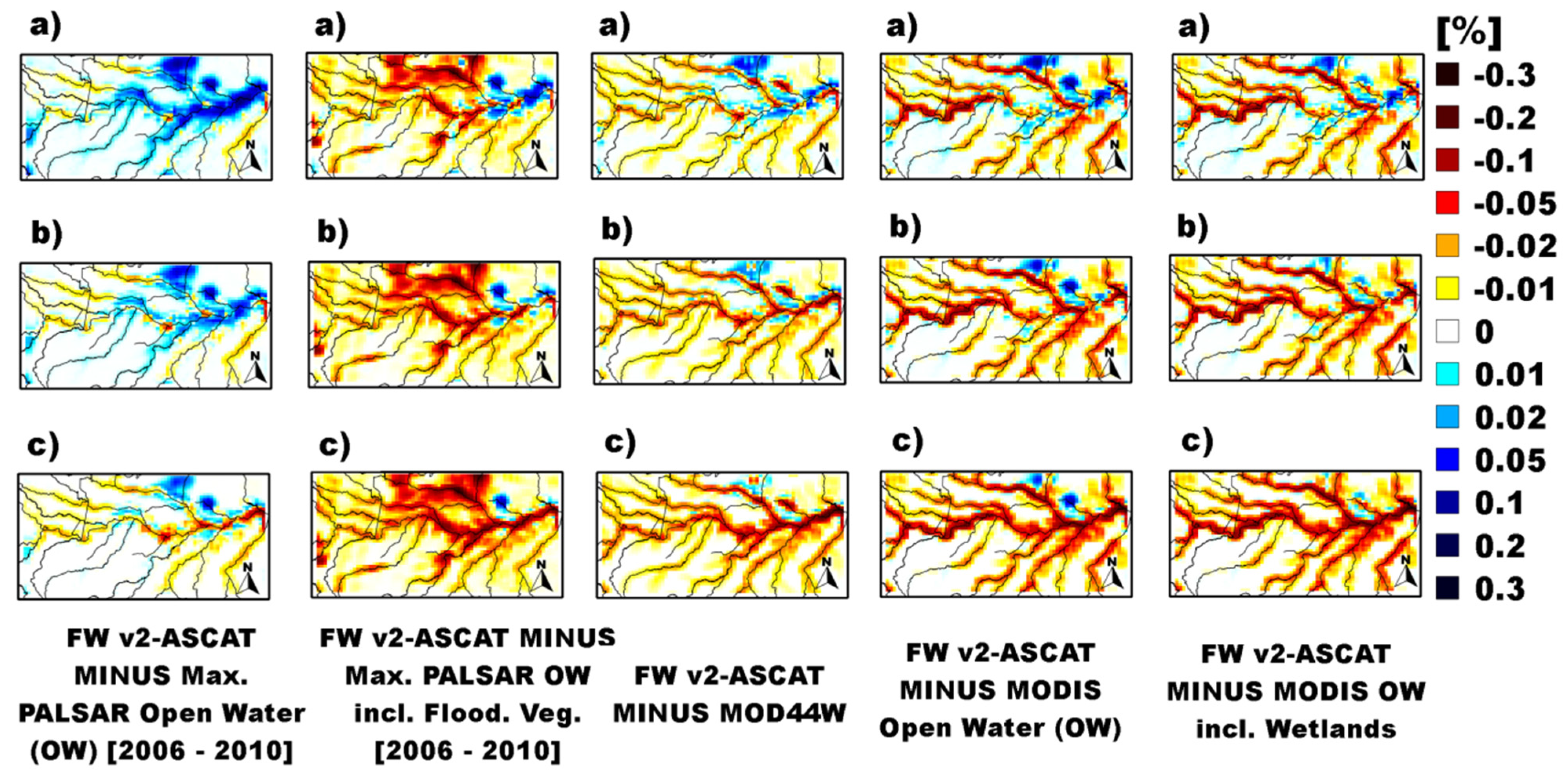
The FW composites were examined for spatial accuracy using the following independent FW products: (1) Open water (OW) bodies and permanent wetlands both from the 1-km global-scale MODIS LC product; (2) 250-m land-water mask from MODIS and the Shuttle Radar Topography Mission’s (SRTM) global-scale Water Body Dataset (MOD44W) [87]; (3) 100-m OW and wetlands derived from the L-band Japanese Earth Resources Satellite (JERS) over the state of Alaska [88] and (4) 100-m maximum OW and flooded forest vegetation (VEG) derived from the Advanced Land Observing Satellite (ALOS) Phased Array type L-band Synthetic Aperture Radar (PALSAR) ScanSAR over the Amazon basin [41]. Water bodies in (1), (2) and (3) do not distinguish ocean from non-ocean water surfaces; (4) distinguishes between VEG, OW/flooded grasses and OW that was occasionally detected. It also provides an ambiguous OW class; this class was not incorporated into the comparison due to difficulty separating OW from bare ground. Maximum FW extent was generated by updating non-inundated grid cells, if in at least one image VEG or OW could be detected. Drop-in-the-bucket averaging was used to produce 25-km EASE-grids from the independent data. We applied a 3 × 3 cell (EASE-grid) weightless box-car filter to these data to account for the larger footprint size (70 × 45 km) of the 19 GHz SSM/I and SSMI/S T_b inputs to SWAMPS. We examined the following measures of spatial correspondence: (1) coefficient of determination (R²) to assess the percentage of spatial variability in the independent data explained by SWAMPS; (2) Mean Residual Error (MRE); and (3) Root Mean Square Error (RMSE) to provide an average bias and accuracy of SWAMPS relative to independent FW. FW from v1-ERS were not included in the comparison against these data because processing of the ERS backscatter data was still ongoing.

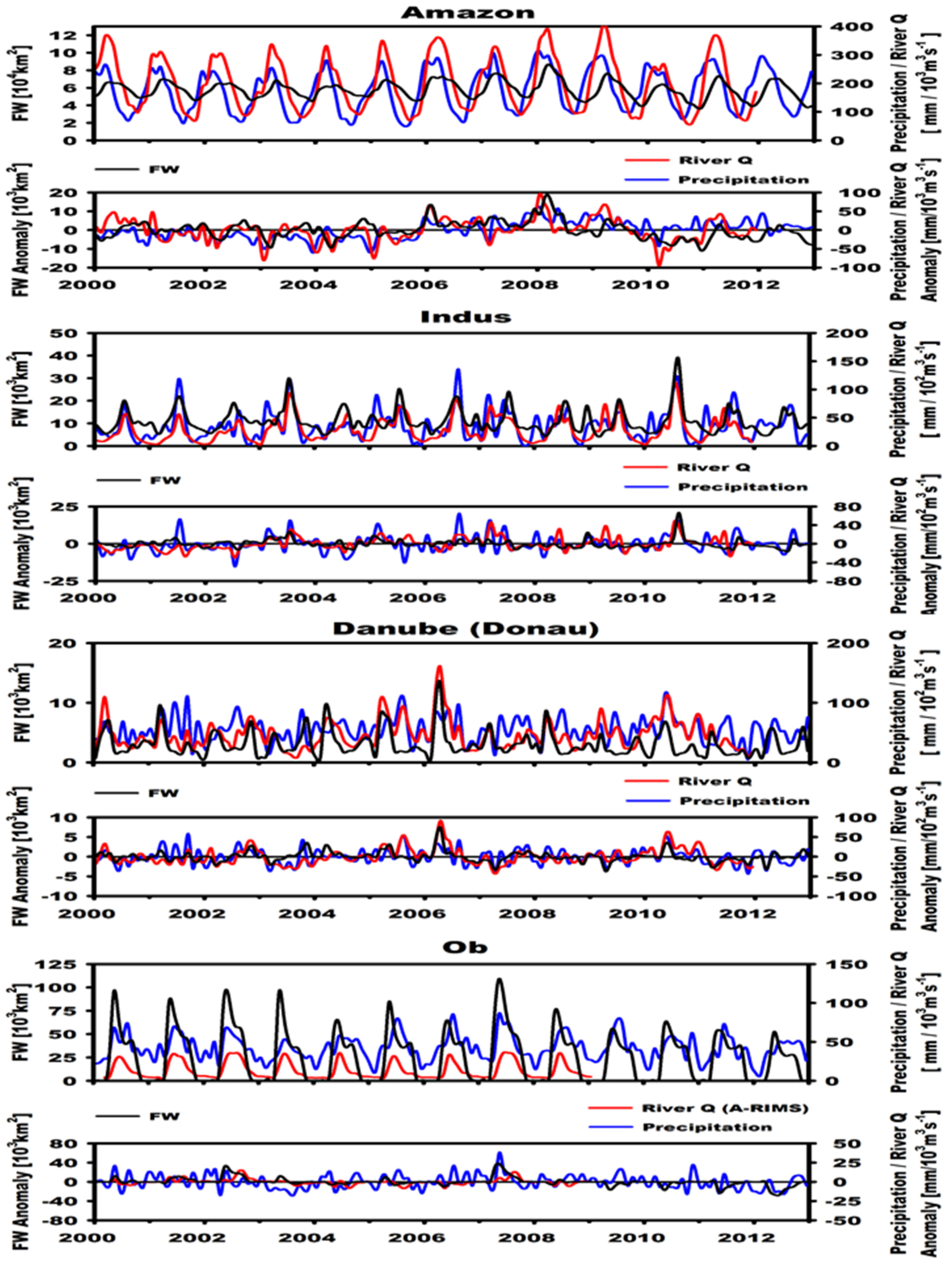
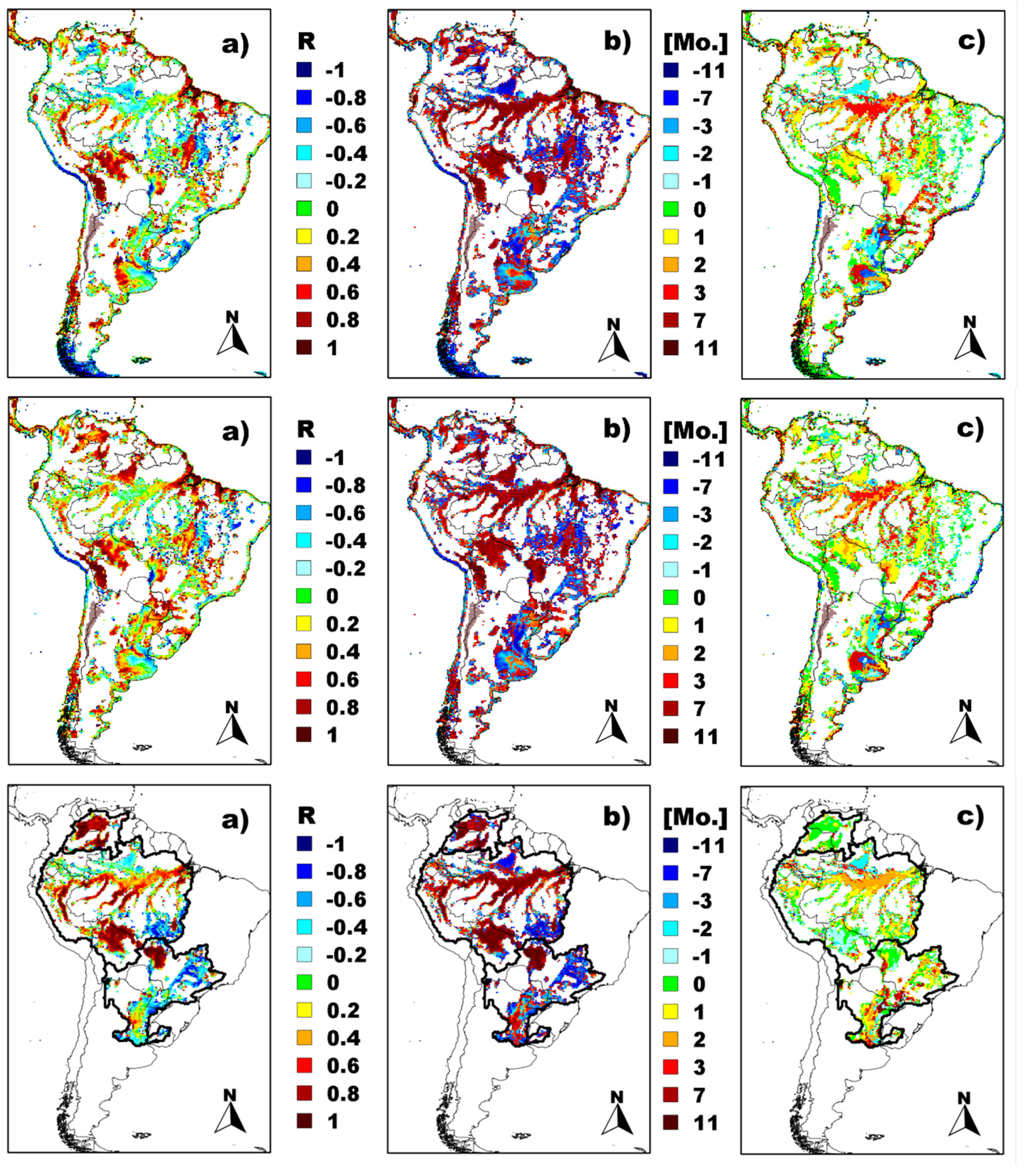
We examined the temporal accuracy of SWAMPS using concurrent precipitation (P) and river discharge (Q) records over major global river basins. Basin-averaged P was computed from the MERRA reanalysis and Q was from either WBM_plus simulations [89] or Arctic-RIMS [90] for the station farthest downstream. We evaluated the following measures of temporal correspondence: (1) the linear correlation coefficient (R); (2) the time-lagged (anomaly) cross-correlation coefficient (R) at maximum absolute correlation; and (3) the corresponding time-lag of the maximum (anomaly) correlation in months. Basin analyses were supported by pixel-wise calculations of R over South America (P only) and within the Amazon, Orinoco and Parana River basins (Q only) to examine lag-patterns between P, FW and Q cycles. 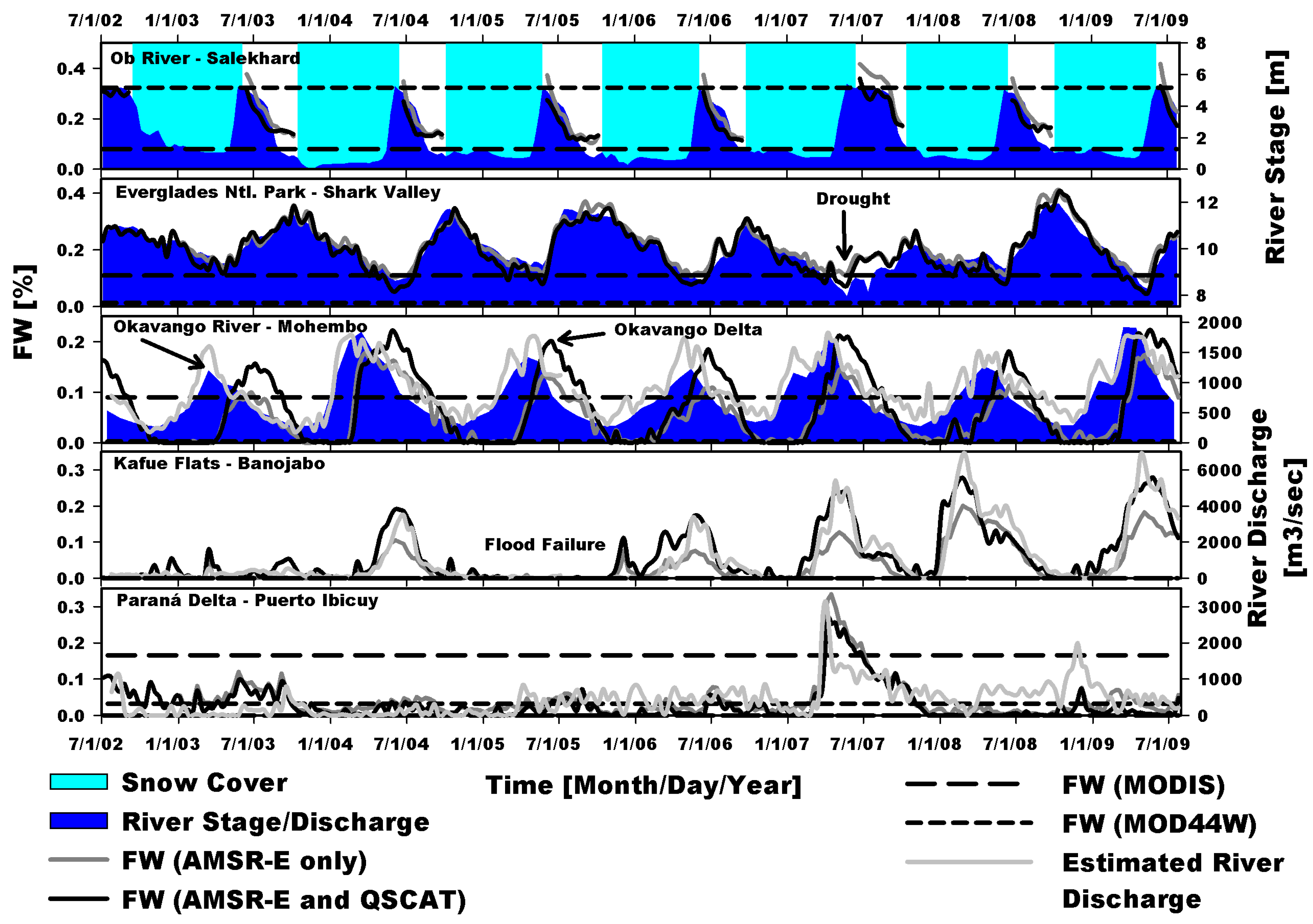P from MERRA was verified via P acquired from the Tropical Rainfall Measurement Mission (TRMM) multi-satellite precipitation analysis (TMPA) [91]. Ten-day average FW records for five global wetland sites were compared against concurrent records of daily river stage height and river Q to assess the ability of the combined AMSR-E/QSCAT record, a prototype version of SWAMPS, to capture seasonal FW variations indicated by the hydrological records. Wetlands sites identified were the Ob River floodplain at Salekhard, Russia (66.53°N, 66.60°E) providing river stage height [90], the Everglades Nat’l Park at Shark Valley, FL, USA (25.76°N, 80.77°W) providing river stage height [92], the Okavango Delta (19.10°S, 22.55°E) providing river discharge from the delta mouth located approximately 120-km upstream at Mohembo River gauging station, Botswana [93], the Kafue Flats at Banojabo, Zambia (15.68°S, 27.58°E) and the Paraná Delta at Puerto Ibicuy, Argentina (33.79°S, 59.19°W) providing satellite estimated river discharge [94,95]. FW variability for these sites was verified with coincident 10-day FW averages derived from AMSR-E [58].

2.5. Trend Analysis and Trend Sensitivity to Snow Cover Screenings

Seasonally adjusted monthly FW extent anomalies from combined FW record periods were generated within the limits of our domain and examined for linear trend by approximating the slope of the least-square best fit-line. Trends were also examined on a grid cell-wise basis by applying linear regression analysis to annual means from combined FW records. Trends were assessed at a minimum 95% probability level; only statistically significant trends (p < 0.05) were mapped. The resulting trend patterns were examined for localized reports of recent changes in surface water area.

High FW often co-occurs with the presence of melting snow packs over still frozen grounds. As a result, conservative snow screening is useful to remove erroneous FW associated with periods of temporary snow melt. We tested the sensitivity of the annual grid cell-wise linear FW trend analysis over the northern hemisphere to variable snow screenings using daily FW records where FW was screened from potential wet snow contamination via (1) a 28-day long sliding mean time domain SWE filter; (2) a 14-day long SWE filter and (3) no filter at all (0-day; only pixels identified by the decision tree were removed). The resulting trend patterns for the 28-, 14- and 0-day snow screened products were mapped and inspected visually for trend variations.

2.6. Quality Control Map

Global FW output from SWAMPS was assessed for FW accuracy relative to sensor retrievals, model results and corresponding satellite-supported P measurements generated from TRMM (supplemented by MERRA at high latitudes). We produced quality control (QC) maps from these records describing grid cell-wise static attributes of FW accuracy within the limits of our domain. Static QC attributes included (1) T_b and σ⁰ temporal coverage (COVER) excluding snow and precipitation events; (2) topographic variability generated from GLOBE; (3) the standard error estimates of the mixture model model predictions for each LC and (4) the plausibility of the sequence (SEQ) of seasonal inundation and precipitation events. To facilitate the first analysis, T_b and σ⁰ temporal gaps, including rain events and seasonal snow cover across the study domain and observation period were recorded. Areas with daily satellite coverage during the snow free season (e.g., high latitudes) and no rain events have the highest temporal coverage (COVER = 100%) while areas with limited satellite coverage and frequent rain events (e.g., tropics) have the lowest temporal coverage. Topographic variability was computed as the standard deviation of all elevation values within a 3 × 3 pixel large moving boxcar, with the lowest score (GLOBE = 0%) for areas with the highest relief variability (e.g., mountain ranges). The accuracy of the model prediction for each LC was estimated from the regression analysis of the passive and active microwave data sets. LC with large emissivity and backscatter variability not caused by seasonal biomass dynamics (e.g., barren land) receive the lowest LC score (LC = 0%). To facilitate the latter analysis, FW and P seasonal cycles were examined for temporal correspondence using phase analysis. For instance, an anti-cyclic sequence where FW decreases as P rises likely reflects modeling errors, whereas cyclic behavior tends to indicate suitable signal un-mixing and favorable FW retrievals. The resulting QC maps were linearly rescaled and aggregated to the final QC map using a weighted mean (50% SEQ, 25% LC, 15% GLOBE, 7.5% T_b and 2.5% σ⁰ COVER). The weights were chosen subjectively with SEQ (COVER) having the largest (smallest) expected impact on overall accuracy.

Table 1. Relationships between Special Sensor Microwave Imager/Sounder (SSMI/S) (v2) and Special Sensor Microwave Imager (SSM/I) (v1) brightness temperatures (K × 10), during mission overlap (2007–2008), for A.M. and P.M. orbital nodes, vertical (V) and horizontal (H) polarizations, and the 19, 22, 37, and 85/91 GHz bands. Relationships are significant at a minimum 0.01 probability level.

Orbital Node	Polarization	19 GHz	22 GHz	37 GHz	85/91 GHz
		[y0(1), a(2), R2(3), RMSE(4), MRE(5)]	[y0(1), a(2), R2(3), RMSE(4), MRE(5)]	[y0(1), a(2), R2(3), RMSE(4), MRE(5)]	[y0(1), a(2), R2(3), RMSE(4), MRE(5)]
AM	V	−85.3136, 1.0464, 0.9930, 38.5677, −36.6085	−69.5971, 1.0342, 0.9953, 22.6536, −20.2809	−40.2823, 1.0128, 0.9959, 12.7900, 6.8048	72.0668, 0.9677, 0.9890, 23.9092, 12.1443
	H	−49.3111, 1.0332, 0.9857, 40.8327, −36.9150		−33.0591, 1.0078, 0.9935, 18.9913, 14.7296	29.2438, 0.9834, 0.9882, 29.9569, 14.5423
PM	V	10.2076, 1.0068, 0.9923, 30.6220, −28.2329	11.0493, 1.0010, 0.9944, 17.0735, −13.6743	13.5759, 0.9894, 0.9951, 19.1385, 12.7735	116.9324, 0.9503, 0.9830, 25.8241, 13.7287
	H	10.9150, 1.0081, 0.9844, 37.2778, −32.2804		20.9808, 0.9857, 0.9924, 23.0815, 16.8249	83.1874, 0.9614, 0.9819, 33.1488, 18.3033

⁽¹⁾intercept ⁽²⁾slope constant ⁽³⁾coefficient of determination ⁽⁴⁾root mean square error ⁽⁵⁾mean residual error

Table 1. Relationships between Special Sensor Microwave Imager/Sounder (SSMI/S) (v2) and Special Sensor Microwave Imager (SSM/I) (v1) brightness temperatures (K × 10), during mission overlap (2007–2008), for A.M. and P.M. orbital nodes, vertical (V) and horizontal (H) polarizations, and the 19, 22, 37, and 85/91 GHz bands. Relationships are significant at a minimum 0.01 probability level.

Orbital Node	Polarization	19 GHz	22 GHz	37 GHz	85/91 GHz
		[y0(1), a(2), R2(3), RMSE(4), MRE(5)]	[y0(1), a(2), R2(3), RMSE(4), MRE(5)]	[y0(1), a(2), R2(3), RMSE(4), MRE(5)]	[y0(1), a(2), R2(3), RMSE(4), MRE(5)]
AM	V	−85.3136, 1.0464, 0.9930, 38.5677, −36.6085	−69.5971, 1.0342, 0.9953, 22.6536, −20.2809	−40.2823, 1.0128, 0.9959, 12.7900, 6.8048	72.0668, 0.9677, 0.9890, 23.9092, 12.1443
	H	−49.3111, 1.0332, 0.9857, 40.8327, −36.9150		−33.0591, 1.0078, 0.9935, 18.9913, 14.7296	29.2438, 0.9834, 0.9882, 29.9569, 14.5423
PM	V	10.2076, 1.0068, 0.9923, 30.6220, −28.2329	11.0493, 1.0010, 0.9944, 17.0735, −13.6743	13.5759, 0.9894, 0.9951, 19.1385, 12.7735	116.9324, 0.9503, 0.9830, 25.8241, 13.7287
	H	10.9150, 1.0081, 0.9844, 37.2778, −32.2804		20.9808, 0.9857, 0.9924, 23.0815, 16.8249	83.1874, 0.9614, 0.9819, 33.1488, 18.3033

⁽¹⁾intercept ⁽²⁾slope constant ⁽³⁾coefficient of determination ⁽⁴⁾root mean square error ⁽⁵⁾mean residual error

3. Results

3.1. Merging the Passive and Active Microwave Satellite Records

The relationship between overlapping T_b records from the SSM/I (v1) and SSMI/S (v2) mission were considerably strong for the successful merging of the two products (Table 1). The RMSE difference between the 19 GHz SSM/I and SSMI/S-band employed in calculating the MPDI was roughly 4 K (3.86 K ≤ RMSE ≤ 4.08 K), with a small negative (cold) bias (i.e., −3.66 K ≤ MRE ≤ 3.69 K) observed for the SSMI/S relative to the SSM/I (Table 1). The observed differences in Table 1 are likely attributable to the cross-sensor calibration [68]. Linear models with the slope and intercept constants (Table 1) were constructed to bias-correct [70] the SSMI/S 19 GHz and remaining frequency bands employed in the screening algorithms.

Similar global patterns of overlapping σ⁰ records from the C-band ASCAT and the K_u-band QSCAT show that the incidence angle and radiometric slope correction applied was sufficient to extend the FW series beyond the QSCAT record (Figure 2).

Figure 2. Global morning overpass radar backscatter from C-band Advanced Scatterometer (ASCAT) (left) and K_u-band QuikSCAT (QSCAT) (right) during July (top row) and backscatter difference between July and January of 2009 (middle row). Actual figure color is a linear interpolation of the colors in the legend. Selected study sites and distribution of dominant vegetated land cover classes as obtained from MODIS LC (bottom panel). All maps in geographic projection. Distance covered by one degree of latitude is approximately 111-km.

Figure 2. Global morning overpass radar backscatter from C-band Advanced Scatterometer (ASCAT) (left) and K_u-band QuikSCAT (QSCAT) (right) during July (top row) and backscatter difference between July and January of 2009 (middle row). Actual figure color is a linear interpolation of the colors in the legend. Selected study sites and distribution of dominant vegetated land cover classes as obtained from MODIS LC (bottom panel). All maps in geographic projection. Distance covered by one degree of latitude is approximately 111-km.

The two products are very similar across the global domain, except in the northern regions during winter and summer. Across the selected comparison sites, the two products’ seasonal cycles (Figure 3) were in most cases similar during snow-free conditions but opposite during snow and frozen ground cover, particularly in spring and fall (e.g., for site T, FT and DN) when the landscape transitioned from predominantly snow covered to snow-free conditions and vice versa.

Figure 3. Daily time series from morning (A.M.) and evening (P.M.) overpasses of C-band ASCAT and K_u-band QSCAT backscatter for 12 selected sites (Figure 2) during mission overlap (11/2008–11/2009).

Figure 3. Daily time series from morning (A.M.) and evening (P.M.) overpasses of C-band ASCAT and K_u-band QSCAT backscatter for 12 selected sites (Figure 2) during mission overlap (11/2008–11/2009).

We attribute the contrasting σ⁰ trends in these sites to the scattering albedo of snow which increases substantially from L- to K_u-band [96]. Likewise, differences in σ⁰ amplitude in sites in the north during summer (e.g., EN, DN and DB) suggest differences in sensitivity to vegetation water content and biomass structure that are attributable to the difference in sensing frequency. We determined that the two products’ time series corresponded best during the evening overpass when all dominant land cover pixels are combined and the landscape was screened for snow (Table 2; pixel-wise correlation coefficients for the entire domain and histograms of R for dominant land covers are provided in Figures S1 and S2). We hypothesize that reduced tissue water content in leaves and related deeper K_u-band canopy penetration in the afternoon (see Frolking et al. [47] for an example of diurnal K_u-band differences in tropical forests (DB)) perhaps explained marginally improved evening temporal correspondences, though exceptions existed (Table 2, Figures S1 and S2). The σ⁰ differences observed between ASCAT and QSCAT suggest that the σ⁰ records cannot be merged without the following restrictions applied prior to the generation of FW: (1) the backscatter time series was screened from snow (2) the σ⁰ end-member calculation was derived separately for each instrument period (e.g., v1-QSCAT and v2-ASCAT) and (3) only the PM overpass data was used, except for ERS whose PM were supplemented by AM overpasses to increase overlap with the passive MW data. Because overlap was still insufficient a 56-day moving average time domain filter was applied to the ERS record.

Table 2. Dominant land cover, # of participating grid cells and A.M. and P.M. minimum, maximum, mean and standard deviation Pearson’s correlation coefficients (R) between overlapping, snow screened and time-averaged daily C-band ASCAT and K_u-band QSCAT backscatter time series data (11/2008–11/2009). Relationships are significant at a minimum 0.01 probability level.

		R
		AM	PM
Land Cover	# Grid Cells	[Min, Max, Mean, StDev]	[Min, Max, Mean, StDev]
EB	16169	−0.83, 0.98, 0.28, 0.38	−0.86, 0.99, 0.24, 0.39
DB	224	−0.76, 0.97, 0.11, 0.54	−0.55, 0.96, 0.31, 0.42
EN	1705	−0.84, 0.98, 0.70, 0.30	−0.41, 0.99, 0.84, 0.15
DN	164	0.21, 0.97, 0.75, 0.13	0.44, 0.99, 0.81, 0.11
WS	927	−0.50, 0.99, 0.77, 0.30	−0.71, 0.99, 0.82, 0.21
SV	1956	0.04, 1.00, 0.95, 0.07	−0.30, 1.00, 0.94, 0.07
GR	6669	−0.87, 1.00, 0.78, 0.30	−0.81, 1.00, 0.80, 0.28
CR	9522	−1.00, 0.99, 0.83, 0.16	−0.54, 1.00, 0.85, 0.15
FT	7	0.53, 0.95, 0.79, 0.17	0.65, 0.98, 0.88, 0.11
T	7190	−1.00, 1.00, 0.62, 0.36	−1.00, 1.00, 0.83, 0.22
CS	14	0.66, 0.97, 0.84, 0.09	0.47, 0.92, 0.79, 0.12
OS	11841	−0.95, 1.00, 0.69, 0.29	−0.92, 1.00, 0.68, 0.29
ALL	56388	−1.00, 1.00, 0.68, 0.26	−1.00, 1.00, 0.73, 0.21

Table 2. Dominant land cover, # of participating grid cells and A.M. and P.M. minimum, maximum, mean and standard deviation Pearson’s correlation coefficients (R) between overlapping, snow screened and time-averaged daily C-band ASCAT and K_u-band QSCAT backscatter time series data (11/2008–11/2009). Relationships are significant at a minimum 0.01 probability level.

		R
		AM	PM
Land Cover	# Grid Cells	[Min, Max, Mean, StDev]	[Min, Max, Mean, StDev]
EB	16169	−0.83, 0.98, 0.28, 0.38	−0.86, 0.99, 0.24, 0.39
DB	224	−0.76, 0.97, 0.11, 0.54	−0.55, 0.96, 0.31, 0.42
EN	1705	−0.84, 0.98, 0.70, 0.30	−0.41, 0.99, 0.84, 0.15
DN	164	0.21, 0.97, 0.75, 0.13	0.44, 0.99, 0.81, 0.11
WS	927	−0.50, 0.99, 0.77, 0.30	−0.71, 0.99, 0.82, 0.21
SV	1956	0.04, 1.00, 0.95, 0.07	−0.30, 1.00, 0.94, 0.07
GR	6669	−0.87, 1.00, 0.78, 0.30	−0.81, 1.00, 0.80, 0.28
CR	9522	−1.00, 0.99, 0.83, 0.16	−0.54, 1.00, 0.85, 0.15
FT	7	0.53, 0.95, 0.79, 0.17	0.65, 0.98, 0.88, 0.11
T	7190	−1.00, 1.00, 0.62, 0.36	−1.00, 1.00, 0.83, 0.22
CS	14	0.66, 0.97, 0.84, 0.09	0.47, 0.92, 0.79, 0.12
OS	11841	−0.95, 1.00, 0.69, 0.29	−0.92, 1.00, 0.68, 0.29
ALL	56388	−1.00, 1.00, 0.68, 0.26	−1.00, 1.00, 0.73, 0.21

3.2. FW Verification and Accuracy Assessment

3.2.1. Spatiotemporal Characteristics of SWAMPS and Relationship with MOD44W and MODIS Incl. Permanent Wetlands

The average annual maximum FW (Figure 4b) compares favorably with the global distribution of static FW from MOD44W (Figure 4a), except for large portions of the Sahara Desert, the Arabian Peninsula and the Levant where SWAMPS’ FW is likely too high. High FW in these regions corresponds with cretaceous outcrops of limestone deposits, e.g., in the Tuwayq Mountains south of the city of Riyadh, Saudi-Arabia [97], whose surface emissivity is much lower than for the majority of desert areas composed of more common minerals (e.g., quartz sand) [98]. Large differences are also evident over parts of Southeast Asia, Eastern China and India for which SWAMPS shows much more FW. High FW in these areas likely corresponds to the seasonal presence of inundation in rice paddies and floodplains not depicted by the MOD44W, whose observation period for this part of the world fell outside the monsoon season [87].

Figure 4. Global maps of fractional water (FW): (a) MOD44W FW; (b–d) the average annual maximum, minimum, and associated standard deviation of the annual means, respectively, of FW, as determined from combined v1-ERS (1992–1999) and v1-QSCAT (2000–2008) monthly means of FW over the global domain. Areas in light grey are outside of the domain, while areas in dark grey represent snow-covered regions. Actual figure color is a linear interpolation of the colors in the legend. Map projection same as Figure 2. Distance covered by one degree of latitude is approximately 111-km.

Figure 4. Global maps of fractional water (FW): (a) MOD44W FW; (b–d) the average annual maximum, minimum, and associated standard deviation of the annual means, respectively, of FW, as determined from combined v1-ERS (1992–1999) and v1-QSCAT (2000–2008) monthly means of FW over the global domain. Areas in light grey are outside of the domain, while areas in dark grey represent snow-covered regions. Actual figure color is a linear interpolation of the colors in the legend. Map projection same as Figure 2. Distance covered by one degree of latitude is approximately 111-km.

The quality control map (Figure 5a) shows regions of very low to very high FW retrieval accuracy. The integrated quality control index is high (>50%) in areas dominated by lakes and river corridors and seasonally inundated wetlands and low (<50%) in many non-inundated arid and semi-arid regions, suggesting that one or multiple quality attributes yielded low values. FW with less and more than 50% of expected FW retrieval quality encompass 17% and 83% of the entire global domain, respectively.

Figure 5. (a) A global quality control map was developed to provide a probabilistic indicator of estimated FW retrieval quality relative to daily sensor coverage, land cover composition, topographic variability and the likelihood of correctly identified seasonal wet and dry cycles. Areas in light grey are outside of the domain, while areas in dark grey represent snow-covered regions. Actual figure color is a linear interpolation of the colors in the legend. Map projection same as Figure 2. Distance covered by one degree of latitude is approximately 111-km. (b) Histograms of fractional water (FW) from MOD44W, MODIS incl. wetlands and the average annual maximum (FWmax) and minimum (FWmin) as determined from combined v1-ERS (1992–1999) and v1-QSCAT (2000–2008) monthly means of FW for the region 50°N60°N to 30°E100°E. Inset figure provides fine-scale resolution for FW > 10%.

Figure 5. (a) A global quality control map was developed to provide a probabilistic indicator of estimated FW retrieval quality relative to daily sensor coverage, land cover composition, topographic variability and the likelihood of correctly identified seasonal wet and dry cycles. Areas in light grey are outside of the domain, while areas in dark grey represent snow-covered regions. Actual figure color is a linear interpolation of the colors in the legend. Map projection same as Figure 2. Distance covered by one degree of latitude is approximately 111-km. (b) Histograms of fractional water (FW) from MOD44W, MODIS incl. wetlands and the average annual maximum (FWmax) and minimum (FWmin) as determined from combined v1-ERS (1992–1999) and v1-QSCAT (2000–2008) monthly means of FW for the region 50°N60°N to 30°E100°E. Inset figure provides fine-scale resolution for FW > 10%.

Small FW (FW < 10%) measured by MOD44W and MODIS across central Russia (Figure 5b), which previously stayed undetected in the GIEMS dataset (cf. Figure 2a, Figure 3c and Figure 4 in Prigent et al. [53]), are well represented in SWAMPS (Figure 4b and Figure 5b). Conversely, medium to large FW (FW ≥ 10%) observed by MOD44W and MODIS across central Russia (Figure 5b), that tended to be overestimated in GIEMS (cf. Figure 2a, Figure 3c and Figure 4 in Prigent et al. [53]), are well within range (Figure 4b and Figure 5b). FW mean dynamic range (Figure 4b,c) is high in the sub-tropical climate zone, particularly across the Indochina Peninsula where monsoon rains and rice cultivation dominate the annual FW cycle. FW interannual variability (Figure 4d) is expectedly higher in the semi-arid climate zone than in other zones, particularly in the African Sahel, Australia’s outback and in the Tigris and Euphrates River valleys. The average maximum annual FW in the Arctic-Boreal occurs in April and May at 50°N and later at higher latitudes coincident with the northward progression of the snowmelt front (Figure 6a) [99]. Average annual maximum inundation in coastal Western Europe occurs during winter in January with an average FW presence of 1–4 months (Figure 6b). The correlation with precipitation (P) is positive and large in Indochina and the Sahel, whereas it is largely negative in the region immediately to the north at the transition from the Sahel into the Saharan Desert (Figure 6c). The reversal of the relationship with P coincides with a sudden jump in the month of maximum inundation with peak FW likely being ahead of time in this zone (Figure 6a). While the maximum FW extent in this region is rather small relative to known wetland areas (Figure 4b), this situation likely indicates modeling errors in semi-arid landscapes (Figure 5a) necessitating post-product screening (Figure 1).

The average annual maximum FW extent for the global domain including the coast stands at 124.7 × 10⁵ km² which compares favorably with the FW extent from MOD44W (123.7 × 10⁵ km²) and MODIS including permanent wetlands (124.9 × 10⁵ km²) (Table 3). While comparable over the entire domain, SWAMPS’ global maximum FW extent excluding the coast (66.1 × 10⁵ km²) is considerably larger than corresponding MOD44W (58.0 × 10⁵ km²) and MODIS (58.5 × 10⁵ km²) suggesting additional FW sensitivity, e.g., in inundated wetlands, that coincides with a systematic dry-bias along the coast. The bias is the result of the differences in the gridding schemes applied to SWAMPS’ T_b and the independent FW data causing the independent data to yield a larger FW value for coasts (cf. Section 3.2.2, Table 4). On a seasonal basis, average FW extent for the global domain is highest in August (101.7 × 10⁵ km²) and lowest in February (77.2 × 10⁵ km²) with an average variability (i.e., standard deviation (SD) of the snow-screened monthly means) of ±15.1 × 10⁵ km² (Table 3). Multiple seasonal maxima of similar magnitude cause a notable displacement of month of occurrence of the seasonal maximum for tropical America and Africa between v1-QSCAT and v2-ASCAT.

Figure 6. Global maps of: (a) the month of average maximum fractional water (FW); (b) the average number of inundated months; (c) the temporal linear correlation (R) between FW and the Modern-Era Retrospective Analysis for Research and Application (MERRA) precipitation analysis and (d) the trend of the annual FW means over the global domain as determine from combined, v1-ERS (1992–1999) and v1-QSCAT (2000–2008) monthly means and total monthly precipitation from the MERRA reanalysis (1992–2008). Actual figure color (c,d) is a linear interpolation of the colors in the legend. Except for (d), areas in white are outside of the domain or are screened (annual mean FW < 1%) from the analysis, while areas in dark grey represent snow covered regions. The annual FW trend was approximated from the slope of the least-square best fit-line and trend significance was assessed at a minimum 95% (p < 0.05) probability level. Only statically significant trends are shown. Map projection same as Figure 2. Distance covered by one degree of latitude is approximately 111-km.

Figure 6. Global maps of: (a) the month of average maximum fractional water (FW); (b) the average number of inundated months; (c) the temporal linear correlation (R) between FW and the Modern-Era Retrospective Analysis for Research and Application (MERRA) precipitation analysis and (d) the trend of the annual FW means over the global domain as determine from combined, v1-ERS (1992–1999) and v1-QSCAT (2000–2008) monthly means and total monthly precipitation from the MERRA reanalysis (1992–2008). Actual figure color (c,d) is a linear interpolation of the colors in the legend. Except for (d), areas in white are outside of the domain or are screened (annual mean FW < 1%) from the analysis, while areas in dark grey represent snow covered regions. The annual FW trend was approximated from the slope of the least-square best fit-line and trend significance was assessed at a minimum 95% (p < 0.05) probability level. Only statically significant trends are shown. Map projection same as Figure 2. Distance covered by one degree of latitude is approximately 111-km.

Table 3. Average seasonal maximum and minimum (including month of occurrence), and annual mean, maximum and minimum fractional water (FW) extents (km² × 10⁵) from SWAMPS over the global and regional domains as generated from v1-ERS (1992–2000), v1-QSCAT (2000–2008) and v2-ASCAT (2009–2012) monthly means. Seasonal and annual variability in inundation extents are expressed as the standard deviation of the snow-screened seasonal climatologies and annual means. The FW extents from static measures of FW from the MOD44W and MODIS including wetlands products are shown for comparison.

Region	Seasonal [v1-ERS/v1-QSCAT/v2-ASCAT]			Annual [v1-ERS/v1-QSCAT/v2-ASCAT]				MOD44W	MODIS incl. Wetlands
	Variability	Maximum [Month]	Minimum [Month]	Variability	Average	Maximum	Minimum
Global	15.7/15.1/14.6	102.2 [8]/101.7 [8]/101.1 [8]	78.6 [2]/77.1 [2]/75.8 [2]	9.0/8.1/7.1	103.0/101.9/100.5	126.8/124.7 /122.7	81.6/81.3 /80.7	123.7	124.9
Global excl. Coast	11.2/10.6/10.2	48.3 [7]/48.3 [6]/48.4 [7]	33.9 [1]/33.0 [1]/33.2 [2]	6.6/5.8/5.0	48.1/47.6/48.2	67.1/65.6 /65.6	34.7/34.9 /36.1	58.0	58.5
Tropical (30S-30N)	5.9/5.8/5.9	48.4 [7]/47.3 [7]/47.0 [7]	44.6 [10]/43.9 [10]/43.3 [10]	3.8/3.3/3.1	46.0/45.3/44.8	56.5/55.6/55.6	38.5/37.9/37.5	49.0	50.4
Tropical excl. Coast	5.0/4.8/4.9	22.5 [7]/21.5 [7]/21.9 [7]	18.9 [10]/18.4 [10]/18.7 [10]	3.2/2.6/2.4	20.2/19.7/20.1	29.4/28.5/29.3	14.1/13.8/14.3	19.6	20.9
Tropical-America (180W-25W)	1.0/1.0/0.9	11.2 [4]/11.1 [3]/11.0 [7]	10.8 [12]/10.7 [12]/10.5 [12]	0.7/0.7/0.7	11.0/10.9/10.8	12.7/12.6/12.4	9.8/9.6/9.6	13.6	14.4
Tropical America excl. Coast	0.7/0.7/0.7	4.4 [3]/4.2 [3]/4.4 [7]	4.0 [12]/3.9 [12]/4.0 [12]	0.5/0.5/0.5	4.2/4.1/4.2	5.5/5.4/5.5	3.3/3.2/3.4	5.7	6.5
Tropical-Africa (25W-50E)	2.3/2.2/2.4	10.5 [7]/10.5 [3]/10.2 [3]	9.0 [9]/8.6 [10]/8.3 [9]	1.6/1.1/1.0	10.0/9.5/9.3	14.0/13.2/13.6	7.0/6.6/6.3	8.6	9.0
Tropical Africa excl. Coast	2.2/2.0/2.2	6.9 [7] /6.9 [3] /7.0 [3]	5.4 [9]/5.0 [9]/5.0 [9]	1.4/1.0/0.9	6.4/5.9/6.0	10.1/9.4/10.0	3.6/3.3/3.3	4.3	4.6
Tropical-Asia (50E-180E)	2.6/2.6/2.5	26.8 [7]/26.7 [7]/26.4 [7]	24.2 [3]/24.2 [2]/24.1 [11]	1.5/1.5/1.4	24.9/24.9/24.7	29.9/29.8/29.6	21.7/21.7/21.6	26.8	27.0
Tropical-Asia excl. Coast	2.1/2.1/2.0	11.4 [7]/11.3 [7]/11.3 [7]	9.0 [3]/9.0 [3]/9.3 [11]	1.2/1.1/1.1	9.6/9.7/9.8	13.8/13.7 / 13.8	7.2/7.3/7.6	9.6	9.8
Arctic-Boreal (> 50 N)	5.8/5.4/5.1	32.1 [9]/31.8 [9]/31.9 [9]	10.3 [2]/10.0 [3]/10.1 [3]	2.8/2.6/2.2	31.3/31.1/31.0	38.1/37.4/36.6	22.9/23.2/23.3	40.6	40.5
Arctic-Boreal excl. Coast	3.4/3.1/2.7	17.0 [9]/16.8 [9]/17.2 [9]	3.9 [2]/3.7 [2]/3.6 [2]	1.7/1.6/1.3	17.0/17.0/17.1	21.7/21.3/20.7	12.9/13.3/13.7	22.2	21.5
N-America (180°W-0°W, > 50 N)	3.3/3.0/3.0	20.4 [9]/20.2 [9]/20.4 [9]	5.5 [2]/5.4 [2]/5.4 [3]	1.6/1.5/1.3	19.6/19.5/19.6	22.9/22.4/22.5	14.4/14.6/14.8	25.3	25.5
N-America excl. Coast	1.7/1.5/1.5	11.0 [9]/10.9 [9]/11.3 [9]	2.0 [2]/1.9 [3]/1.9 [3]	0.9/0.8/0.7	10.7/10.7/10.9	12.6/12.4/12.5	8.1/8.5/8.8	13.7	13.5
Eurasia (0°E-180°E, > 50 N)	2.5/2.4/2.1	11.7 [9]/11.7 [9]/11.5 [9]	4.8 [2]/4.6 [3]/4.6 [2]	1.2/1.1/0.9	11.7/11.6/11.4	15.2/14.9/14.1	8.5/8.6/8.5	15.3	15.0
Eurasia excl. Coast	1.7/1.6/1.2	6.2 [6]/6.3 [6]/5.9 [6]	1.9 [2]/1.8 [2]/1.6 [2]	0.8/0.8/0.6	6.4/6.3/6.2	9.1/8.9/8.2	4.8/4.8/4.9	8.5	8.0

Table 3. Average seasonal maximum and minimum (including month of occurrence), and annual mean, maximum and minimum fractional water (FW) extents (km² × 10⁵) from SWAMPS over the global and regional domains as generated from v1-ERS (1992–2000), v1-QSCAT (2000–2008) and v2-ASCAT (2009–2012) monthly means. Seasonal and annual variability in inundation extents are expressed as the standard deviation of the snow-screened seasonal climatologies and annual means. The FW extents from static measures of FW from the MOD44W and MODIS including wetlands products are shown for comparison.

Region	Seasonal [v1-ERS/v1-QSCAT/v2-ASCAT]			Annual [v1-ERS/v1-QSCAT/v2-ASCAT]				MOD44W	MODIS incl. Wetlands
	Variability	Maximum [Month]	Minimum [Month]	Variability	Average	Maximum	Minimum
Global	15.7/15.1/14.6	102.2 [8]/101.7 [8]/101.1 [8]	78.6 [2]/77.1 [2]/75.8 [2]	9.0/8.1/7.1	103.0/101.9/100.5	126.8/124.7 /122.7	81.6/81.3 /80.7	123.7	124.9
Global excl. Coast	11.2/10.6/10.2	48.3 [7]/48.3 [6]/48.4 [7]	33.9 [1]/33.0 [1]/33.2 [2]	6.6/5.8/5.0	48.1/47.6/48.2	67.1/65.6 /65.6	34.7/34.9 /36.1	58.0	58.5
Tropical (30S-30N)	5.9/5.8/5.9	48.4 [7]/47.3 [7]/47.0 [7]	44.6 [10]/43.9 [10]/43.3 [10]	3.8/3.3/3.1	46.0/45.3/44.8	56.5/55.6/55.6	38.5/37.9/37.5	49.0	50.4
Tropical excl. Coast	5.0/4.8/4.9	22.5 [7]/21.5 [7]/21.9 [7]	18.9 [10]/18.4 [10]/18.7 [10]	3.2/2.6/2.4	20.2/19.7/20.1	29.4/28.5/29.3	14.1/13.8/14.3	19.6	20.9
Tropical-America (180W-25W)	1.0/1.0/0.9	11.2 [4]/11.1 [3]/11.0 [7]	10.8 [12]/10.7 [12]/10.5 [12]	0.7/0.7/0.7	11.0/10.9/10.8	12.7/12.6/12.4	9.8/9.6/9.6	13.6	14.4
Tropical America excl. Coast	0.7/0.7/0.7	4.4 [3]/4.2 [3]/4.4 [7]	4.0 [12]/3.9 [12]/4.0 [12]	0.5/0.5/0.5	4.2/4.1/4.2	5.5/5.4/5.5	3.3/3.2/3.4	5.7	6.5
Tropical-Africa (25W-50E)	2.3/2.2/2.4	10.5 [7]/10.5 [3]/10.2 [3]	9.0 [9]/8.6 [10]/8.3 [9]	1.6/1.1/1.0	10.0/9.5/9.3	14.0/13.2/13.6	7.0/6.6/6.3	8.6	9.0
Tropical Africa excl. Coast	2.2/2.0/2.2	6.9 [7] /6.9 [3] /7.0 [3]	5.4 [9]/5.0 [9]/5.0 [9]	1.4/1.0/0.9	6.4/5.9/6.0	10.1/9.4/10.0	3.6/3.3/3.3	4.3	4.6
Tropical-Asia (50E-180E)	2.6/2.6/2.5	26.8 [7]/26.7 [7]/26.4 [7]	24.2 [3]/24.2 [2]/24.1 [11]	1.5/1.5/1.4	24.9/24.9/24.7	29.9/29.8/29.6	21.7/21.7/21.6	26.8	27.0
Tropical-Asia excl. Coast	2.1/2.1/2.0	11.4 [7]/11.3 [7]/11.3 [7]	9.0 [3]/9.0 [3]/9.3 [11]	1.2/1.1/1.1	9.6/9.7/9.8	13.8/13.7 / 13.8	7.2/7.3/7.6	9.6	9.8
Arctic-Boreal (> 50 N)	5.8/5.4/5.1	32.1 [9]/31.8 [9]/31.9 [9]	10.3 [2]/10.0 [3]/10.1 [3]	2.8/2.6/2.2	31.3/31.1/31.0	38.1/37.4/36.6	22.9/23.2/23.3	40.6	40.5
Arctic-Boreal excl. Coast	3.4/3.1/2.7	17.0 [9]/16.8 [9]/17.2 [9]	3.9 [2]/3.7 [2]/3.6 [2]	1.7/1.6/1.3	17.0/17.0/17.1	21.7/21.3/20.7	12.9/13.3/13.7	22.2	21.5
N-America (180°W-0°W, > 50 N)	3.3/3.0/3.0	20.4 [9]/20.2 [9]/20.4 [9]	5.5 [2]/5.4 [2]/5.4 [3]	1.6/1.5/1.3	19.6/19.5/19.6	22.9/22.4/22.5	14.4/14.6/14.8	25.3	25.5
N-America excl. Coast	1.7/1.5/1.5	11.0 [9]/10.9 [9]/11.3 [9]	2.0 [2]/1.9 [3]/1.9 [3]	0.9/0.8/0.7	10.7/10.7/10.9	12.6/12.4/12.5	8.1/8.5/8.8	13.7	13.5
Eurasia (0°E-180°E, > 50 N)	2.5/2.4/2.1	11.7 [9]/11.7 [9]/11.5 [9]	4.8 [2]/4.6 [3]/4.6 [2]	1.2/1.1/0.9	11.7/11.6/11.4	15.2/14.9/14.1	8.5/8.6/8.5	15.3	15.0
Eurasia excl. Coast	1.7/1.6/1.2	6.2 [6]/6.3 [6]/5.9 [6]	1.9 [2]/1.8 [2]/1.6 [2]	0.8/0.8/0.6	6.4/6.3/6.2	9.1/8.9/8.2	4.8/4.8/4.9	8.5	8.0

3.2.2. Global Comparisons of SWAMPS with MOD44W and MODIS

Average annual FW generated from monthly mean (FW_ave), maximum (FW_max) and minimum (FW_min) record periods over the global domain all explain the majority of spatial variability (80.5% ≤ R² ≤ 93.9%) in the MOD44W and MODIS static FW maps, except along the coast and shoreline of large water bodies where SWAMPS yields much lower FW (−33.8% ≤ MRE ≤ 8.2%) (Table 4, Figure 7). The average RMSE difference between SWAMPS’ FW_ave and FW_max, and MOD44W over the Arctic-Boreal excluding the coast is ≤5%, in line with the results from Watts et al. [64]. Pixel correspondences are lower between SWAMPS and MODIS than between SWAMPS and MOD44W, particularly along the coast where MOD44W (61.3% ≤ R² ≤ 78.8%) was expected to outperform MODIS (52.1% ≤ R² ≤ 75.0%) (Table 4).

Table 4. Summary statistics from pixel-wise comparisons of mean annual fractional water (FW) generated from v1-QSCAT (2000–2008) and v2-ASCAT (2009–2012) monthly maximum (FW_max), average (FW_ave), and minimum (FW_min) record periods against static FW from the MOD44W and MODIS including wetlands products. Relationships are significant at a minimum 0.01 probability level.

Data Set	Coefficient of Determination [%] v-QSCAT/v2-ASCAT			Mean Residual Error [%] V1-QSCAT/v2-ASCAT			Root Mean Square Error [%] V1-QSCAT/v2-ASCAT
Region	FWmax	FWave	FWmin	FWmax	FWave	FWmin	FWmax	FWave	FWmin
MOD44W
Arctic-Boreal (> 50 N)	91.4/92.0	91.5/91.0	83.8/88.8	2.1/−1.0	−2.9/−2.9	−6.9/−5.0	6.8/6.1	7.7/8.0	13.9/11.1
Arctic-Boreal excl. Coast	87.9/88.4	88.2/88.1	76.3/86.3	1.9/−0.4	−1.8/−1.7	−4.3/−3.0	5.4/4.3	5.2/5.1	9.0/6.8
Global	92.3/93.9	92.1/93.5	81.1/91.5	2.8/0.3	−1.5/−1.6	−5.0/−3.5	6.8/5.0	6.3/6.2	12.2/9.0
Global excl. Coast	84.1/86.2	84.0/87.3	67.8/85.5	2.5/0.7	−0.8/−0.7	−2.9/−1.9	5.7/4.1	4.8/4.4	8.1/5.8
Global excl. Coast & Desert	85.6/88.4	85.0/89.1	70.6/87.2	2.2/0.3	−1.1/−1.0	−3.3/−2.2	5.5/3.9	4.9/4.5	8.5/6.1
Global Coast only	61.3/79.2	72.2/78.8	64.4/74.0	8.2/−4.5	−11.3/−13.8	−33.6/−25.0	15.1/10.6	15.7/16.7	35.7/26.8
MODIS incl. Wetlands
Arctic-Boreal (> 50 N)	88.6/90.8	89.3/89.9	82.4/88.1	2.1/−0.9	−2.8/−2.9	−6.8/−5.0	7.7/6.5	8.1/8.1	14.0/11.0
Arctic-Boreal excl. Coast	84.6/86.5	85.9/86.5	75.1/85.3	2.2/−0.1	−1.5/−1.5	−4.1/−2.8	6.1/4.4	5.1/5.0	8.6/6.4
Global	91.2/93.1	91.3/92.7	80.5/90.0	2.8/0.3	−1.6/−1.7	−5.0/−3.5	7.2/5.2	6.5/6.4	12.2/9.1
Global excl. Coast	82.6/85.0	82.8/86.2	67.0/84.6	2.4/0.6	−0.8/−0.8	−2.9/−2.0	5.9/4.2	4.8/4.5	8.0/5.8
Global excl. Coast & Desert	84.2/87.3	84.7/88.1	69.7/86.3	2.1/0.3	−1.2/−1.1	−3.3/−2.2	5.7/4.0	5.0/4.5	8.4/6.0
Global Coast only	52.1/74.3	67.3/75.0	64.0/71.2	8.0/−4.8	−11.6/−14.0	−33.8/−25.2	16.1/11.6	16.4/17.3	35.9/27.2

Table 4. Summary statistics from pixel-wise comparisons of mean annual fractional water (FW) generated from v1-QSCAT (2000–2008) and v2-ASCAT (2009–2012) monthly maximum (FW_max), average (FW_ave), and minimum (FW_min) record periods against static FW from the MOD44W and MODIS including wetlands products. Relationships are significant at a minimum 0.01 probability level.

Data Set	Coefficient of Determination [%] v-QSCAT/v2-ASCAT			Mean Residual Error [%] V1-QSCAT/v2-ASCAT			Root Mean Square Error [%] V1-QSCAT/v2-ASCAT
Region	FWmax	FWave	FWmin	FWmax	FWave	FWmin	FWmax	FWave	FWmin
MOD44W
Arctic-Boreal (> 50 N)	91.4/92.0	91.5/91.0	83.8/88.8	2.1/−1.0	−2.9/−2.9	−6.9/−5.0	6.8/6.1	7.7/8.0	13.9/11.1
Arctic-Boreal excl. Coast	87.9/88.4	88.2/88.1	76.3/86.3	1.9/−0.4	−1.8/−1.7	−4.3/−3.0	5.4/4.3	5.2/5.1	9.0/6.8
Global	92.3/93.9	92.1/93.5	81.1/91.5	2.8/0.3	−1.5/−1.6	−5.0/−3.5	6.8/5.0	6.3/6.2	12.2/9.0
Global excl. Coast	84.1/86.2	84.0/87.3	67.8/85.5	2.5/0.7	−0.8/−0.7	−2.9/−1.9	5.7/4.1	4.8/4.4	8.1/5.8
Global excl. Coast & Desert	85.6/88.4	85.0/89.1	70.6/87.2	2.2/0.3	−1.1/−1.0	−3.3/−2.2	5.5/3.9	4.9/4.5	8.5/6.1
Global Coast only	61.3/79.2	72.2/78.8	64.4/74.0	8.2/−4.5	−11.3/−13.8	−33.6/−25.0	15.1/10.6	15.7/16.7	35.7/26.8
MODIS incl. Wetlands
Arctic-Boreal (> 50 N)	88.6/90.8	89.3/89.9	82.4/88.1	2.1/−0.9	−2.8/−2.9	−6.8/−5.0	7.7/6.5	8.1/8.1	14.0/11.0
Arctic-Boreal excl. Coast	84.6/86.5	85.9/86.5	75.1/85.3	2.2/−0.1	−1.5/−1.5	−4.1/−2.8	6.1/4.4	5.1/5.0	8.6/6.4
Global	91.2/93.1	91.3/92.7	80.5/90.0	2.8/0.3	−1.6/−1.7	−5.0/−3.5	7.2/5.2	6.5/6.4	12.2/9.1
Global excl. Coast	82.6/85.0	82.8/86.2	67.0/84.6	2.4/0.6	−0.8/−0.8	−2.9/−2.0	5.9/4.2	4.8/4.5	8.0/5.8
Global excl. Coast & Desert	84.2/87.3	84.7/88.1	69.7/86.3	2.1/0.3	−1.2/−1.1	−3.3/−2.2	5.7/4.0	5.0/4.5	8.4/6.0
Global Coast only	52.1/74.3	67.3/75.0	64.0/71.2	8.0/−4.8	−11.6/−14.0	−33.8/−25.2	16.1/11.6	16.4/17.3	35.9/27.2

FW_max has a small wet bias relative to static FW (Table 4, Figure 7a), whereas FW_ave and FW_min show small-to-large dry-biasing (Table 4, Figure 7b,c). The FW_max and FW_min bias from v1-QSCAT is larger than the corresponding bias from v2-ASCAT, except when the MRE is generated from FW_ave where v1 and v2 biasing is similar. The product differences for these measures are consistent with the differences in the gridding procedure reported for the v1 and v2 T_b data [68]. Regionally, FW_max, FW_ave and FW_min from v1 and v2 are lower than static FW along major river ways (e.g., Ob River), lakes and reservoirs (e.g., Central Canada) (Figure 7). Conversely, FW_max, FW_ave and FW_min are greater than static FW in arid regions and the wetland-dominated areas (e.g., WSL, Everglades).

Figure 7. Difference maps between average annual fractional water (FW) from v1-QSCAT (2000–2008, left) and v2-ASCAT (2009–2012, right) generated from (a) monthly maximum (FW_max), (b) monthly average (FW_ave) and (c) monthly minimum (FW_min) minus static FW from the MOD44W (top) and the MODIS including permanent wetlands product (bottom) for the entire domain. Areas in light grey are outside of the domain, while areas in dark grey represent snow-covered regions. Actual figure color is a linear interpolation of the colors in the legend. Map projection same as Figure 2. Distance covered by one degree of latitude is approximately 111-km.

Figure 7. Difference maps between average annual fractional water (FW) from v1-QSCAT (2000–2008, left) and v2-ASCAT (2009–2012, right) generated from (a) monthly maximum (FW_max), (b) monthly average (FW_ave) and (c) monthly minimum (FW_min) minus static FW from the MOD44W (top) and the MODIS including permanent wetlands product (bottom) for the entire domain. Areas in light grey are outside of the domain, while areas in dark grey represent snow-covered regions. Actual figure color is a linear interpolation of the colors in the legend. Map projection same as Figure 2. Distance covered by one degree of latitude is approximately 111-km.

The seasonal progression for 20+ years of monthly FW extents in the Arctic-Boreal shows that the change in backscatter sensing frequency among the products generated did not introduce a record discontinuity, except for lower FW_max and higher FW_min beginning in 2008/2009 coincident with lower MDPI_max and higher MPDI_min resulting from the change in the T_b gridding procedure (Figure 8). Continuity of the FW time series is demonstrated during 18 months of FW co-retrieval (v1-ERS/v1-QSCAT) for which all three FW measures overlap seamlessly (Figure 8). Figure 8 suggests that the differences in FW extent for FW_max and FW_min in the Arctic-Boreal can be mitigated by determining the FW extent from a temporal composite of multiple (daily) observations (e.g., monthly means). Day-to-day FW variability (i.e., the grid noise) for each gridding procedure is evidently very different. It is caused by swath footprints (roughly 40 × 70 km) whose small position offsets cause differences in footprint open water fraction when combined into 25 km grid cells along water bodies. Therefore, care should be taken when comparing FW from v1 with FW from v2, particularly along the coast.

Figure 8. Seasonal progression of monthly FW extents (km²) from SWAMPS and total Microwave Polarization Difference Index (MPDI) in the Arctic-Boreal domain (>50°N) as generated from monthly maximum (FW_max, MPDI_max) average (FW_ave, MPDI_ave) and minimum (FW_min, MPDI_min) for the study period (1992–2013). The Arctic-Boreal FW extent from static measures of FW from the MOD44W and MODIS including wetlands products are shown for comparison. Note that FW has been plotted from all record periods including duplicate measurements taken during period overlap.

Figure 8. Seasonal progression of monthly FW extents (km²) from SWAMPS and total Microwave Polarization Difference Index (MPDI) in the Arctic-Boreal domain (>50°N) as generated from monthly maximum (FW_max, MPDI_max) average (FW_ave, MPDI_ave) and minimum (FW_min, MPDI_min) for the study period (1992–2013). The Arctic-Boreal FW extent from static measures of FW from the MOD44W and MODIS including wetlands products are shown for comparison. Note that FW has been plotted from all record periods including duplicate measurements taken during period overlap.

Pixel-wise global-scale comparisons of FW generated from v1-QSCAT against corresponding FW records from v1-ERS and v2-ASCAT confirm high spatial correspondence among the products generated, except for the coast over which v2-ASCAT is dry-biased relative to v1-QSCAT and v1-ERS (Table 5). v1-ERS was not compared with v2-ASCAT because both v1-ERS and v1-QSCAT show a very high degree of correspondence. We attribute this bias to the change in the gridding procedure and associated large T_b differences reported for coasts and other high-gradient T_b regions [68]. These differences can be one or two grid cells wide [68] implying that FW from v2-ASCAT located inland but closest to the coast is likely wet-biased relative to v1-QSCAT and v1-ERS.

Table 5. Summary statistics from pixel-wise comparisons of average annual mean, maximum and minimum fractional water (FW) generated from v1-QSCAT (2000–2008) against corresponding FW record from v1-ERS (1992–2000) and v2-ASCAT (2009–2012) over the global domain, by excluding coastal regions and for coastal regions alone. Relationships are significant at a minimum 0.01 probability level.

	Coefficient of Determination [%]	Mean Residual Error [%]	Root Mean Square Error [%]	Coefficient of Determination [%]	Mean Residual Error [%]	Root Mean Square Error [%]
Data Set	v1-QSCAT – v1-ERS			v1-QSCAT – v2-ASCAT
Region
Global
Average Annual Mean	99.3	−0.07	1.3	98.3	0.11	2.2
Average Annual Maximum	98.7	−0.15	2.0	97.7	0.14	2.7
Average Annual Minimum	98.3	−0.02	1.9	97.3	0.04	2.4
Global excl. Coast
Average Annual Mean	98.8	−0.04	0.9	96.5	−0.05	1.6
Average Annual Maximum	96.8	−0.11	1.6	94.9	0.00	2.1
Average Annual Minimum	97.5	0.02	1.1	95.1	−0.10	1.6
Global Coast only
Average Annual Mean	98.1	−0.03	2.8	93.4	2.48	5.8
Average Annual Maximum	96.4	−0.13	3.8	91.9	2.48	6.4
Average Annual Minimum	94.4	−0.18	5.5	91.7	2.14	7.0

Table 5. Summary statistics from pixel-wise comparisons of average annual mean, maximum and minimum fractional water (FW) generated from v1-QSCAT (2000–2008) against corresponding FW record from v1-ERS (1992–2000) and v2-ASCAT (2009–2012) over the global domain, by excluding coastal regions and for coastal regions alone. Relationships are significant at a minimum 0.01 probability level.

	Coefficient of Determination [%]	Mean Residual Error [%]	Root Mean Square Error [%]	Coefficient of Determination [%]	Mean Residual Error [%]	Root Mean Square Error [%]
Data Set	v1-QSCAT – v1-ERS			v1-QSCAT – v2-ASCAT
Region
Global
Average Annual Mean	99.3	−0.07	1.3	98.3	0.11	2.2
Average Annual Maximum	98.7	−0.15	2.0	97.7	0.14	2.7
Average Annual Minimum	98.3	−0.02	1.9	97.3	0.04	2.4
Global excl. Coast
Average Annual Mean	98.8	−0.04	0.9	96.5	−0.05	1.6
Average Annual Maximum	96.8	−0.11	1.6	94.9	0.00	2.1
Average Annual Minimum	97.5	0.02	1.1	95.1	−0.10	1.6
Global Coast only
Average Annual Mean	98.1	−0.03	2.8	93.4	2.48	5.8
Average Annual Maximum	96.4	−0.13	3.8	91.9	2.48	6.4
Average Annual Minimum	94.4	−0.18	5.5	91.7	2.14	7.0

3.2.3. Direct Comparison of SWAMPS with JERS-SAR and ALOS-PALSAR ScanSAR over Alaska and the Central Amazon Basin

Average annual maximum (FW_max), mean (FW_ave) and minimum (FW_min) FW generated from monthly mean record periods over the state of Alaska explain the majority of spatial variability (86.2 ≤ R² ≤ 97.2) in the JERS OW (284,000 km²), MOD44W (287,000 km²) and MODIS (276,000 km²) static FW maps, except for the wetland portion (70,000 km²) of the combined longer wavelength JERS classification (354,000 km²) where SWAMPS (183,000–256,000 km²) yields much lower FW (−11.4 ≤ MRE ≤ −6.5) (Table 6, Figure 9). Pixel correspondences between SWAMPS and static FW are slightly lower for the comparison against JERS-SAR OW and MODIS than MOD44W.

FW_max has a small dry-bias relative to static FW, whereas FW_ave and FW_min show larger dry-biasing. FW from v2-ASCAT is consistently dry-biased relative to v1-QSCAT. The bias is most notable along the coast (Figure 9) consistent with the above mentioned T_b gridding differences. Locally, FW_max, FW_ave and FW_min are lower than static FW from MOD44W and JERS-SAR OW in the North Slope as well as in portions of the southern Yukon Delta (Figure 9). Conversely, FW_max, FW_ave and FW_min in these areas are higher than static FW from MODIS. In other regions, such as the maritime and glaciated south, FW_max, FW_ave and FW_min are higher than static FW, except for the comparison against MODIS which yields higher FW.

Table 6. Areal extent and summary statistics from pixel-wise comparisons of fractional water (FW) generated from v1-QSCAT (2000–2008) and v2-ASCAT (2009–2012) average annual maximum (FW_max), mean (FW_ave), and minimum (FW_min) record periods against maps of open water (OW) and wetlands derived from the L-band Japanese Earth Resources Satellite (JERS)-based Alaska wetland map and static FW from the MOD44W and MODIS including wetlands products over the state of Alaska (54°N–72°N, 143°W–170°W). Relationships are significant at a minimum 0.01 probability level.

Areal Extent [km2 × 103]

Coefficient of Determination [%]

Mean Residual Error [%]

Root Mean Square Error [%]

Data Set

v1-QSCAT/v2-ASCAT

v1-QSCAT/v2-ASCAT

v1-QSCAT/v2-ASCAT

v1-QSCAT/v2-ASCAT

FWmax

FWave

FWmin

FWmax

FWave

FWmin

FWmax

FWave

FWmin

FWmax

FWave

FWmin

255.5/248.3

228.0/221.4

194.9/183.4

JERS Open Water (OW)

284.1

93.0/94.2

93.4/94.4

87.6/86.2

−1.9/−2.4

−3.7/−4.2

−5.9/−6.7

7.9/7.8

9.0/9.3

12.5/14.0

JERS OW incl. Wetlands

353.7

85.3/87.3

85.2/87.2

78.2/77.9

−6.5/−7.1

−8.4/−8.9

−10.6/−11.4

13.2/13.1

14.6/14.8

18.0/19.1

MOD44W

286.6

96.4/97.2

96.5/97.0

90.0/87.8

−2.1/−2.6

−3.9/−4.4

−6.1/−6.9

5.7/5.7

7.0/7.6

11.2/12.8

MODIS Open Water (OW)

275.9

96.2/96.3

96.1/95.9

90.5/87.5

−1.3/−1.8

−3.2/−3.6

−5.4/−6.1

5.1/5.3

6.2/6.9

10.0/11.7

MODIS OW incl. Wetlands

276.2

96.2/96.3

96.1/95.9

90.5/87.6

−1.4/−1.8

−3.2/−3.6

−5.4/−6.1

5.1/5.3

6.3/7.0

10.0/11.8

Table 6. Areal extent and summary statistics from pixel-wise comparisons of fractional water (FW) generated from v1-QSCAT (2000–2008) and v2-ASCAT (2009–2012) average annual maximum (FW_max), mean (FW_ave), and minimum (FW_min) record periods against maps of open water (OW) and wetlands derived from the L-band Japanese Earth Resources Satellite (JERS)-based Alaska wetland map and static FW from the MOD44W and MODIS including wetlands products over the state of Alaska (54°N–72°N, 143°W–170°W). Relationships are significant at a minimum 0.01 probability level.

Areal Extent [km2 × 103]

Coefficient of Determination [%]

Mean Residual Error [%]

Root Mean Square Error [%]

Data Set

v1-QSCAT/v2-ASCAT

v1-QSCAT/v2-ASCAT

v1-QSCAT/v2-ASCAT

v1-QSCAT/v2-ASCAT

FWmax

FWave

FWmin

FWmax

FWave

FWmin

FWmax

FWave

FWmin

FWmax

FWave

FWmin

255.5/248.3

228.0/221.4

194.9/183.4

JERS Open Water (OW)

284.1

93.0/94.2

93.4/94.4

87.6/86.2

−1.9/−2.4

−3.7/−4.2

−5.9/−6.7

7.9/7.8

9.0/9.3

12.5/14.0

JERS OW incl. Wetlands

353.7

85.3/87.3

85.2/87.2

78.2/77.9

−6.5/−7.1

−8.4/−8.9

−10.6/−11.4

13.2/13.1

14.6/14.8

18.0/19.1

MOD44W

286.6

96.4/97.2

96.5/97.0

90.0/87.8

−2.1/−2.6

−3.9/−4.4

−6.1/−6.9

5.7/5.7

7.0/7.6

11.2/12.8

MODIS Open Water (OW)

275.9

96.2/96.3

96.1/95.9

90.5/87.5

−1.3/−1.8

−3.2/−3.6

−5.4/−6.1

5.1/5.3

6.2/6.9

10.0/11.7

MODIS OW incl. Wetlands

276.2

96.2/96.3

96.1/95.9

90.5/87.6

−1.4/−1.8

−3.2/−3.6

−5.4/−6.1

5.1/5.3

6.3/7.0

10.0/11.8

Table 7. Areal extent and summary statistics from pixel-wise comparisons of fractional water (FW) generated from v1-QSCAT (2000–2008) and v2-ASCAT (2009–2012) average annual maximum (FW_max), mean (FW_ave), and minimum (FW_min) record periods against maps of open water (OW) and flooded vegetation derived from the Advanced Land Observing Satellite (ALOS) Phased Array type L-band Synthetic Aperture Radar (PALSAR) ScanSAR Amazon maximum inundation extent map and subsets of static FW from the MOD44W and MODIS including wetlands products for a section (8.5°S–1°N, 55.5°W–74.5°W) of the central Amazon river floodplain. Relationships are significant at a minimum 0.01 probability level.

Areal Extent [km2 × 103]

Coefficient of Determination [%]

Mean Residual Error [%]

Root Mean Square Error [%]

Data Set

v1-QSCAT/v2-ASCAT

v1-QSCAT/v2-ASCAT

v1-QSCAT/v2-ASCAT

v1-QSCAT/v2-ASCAT

FWmax

FWave

FWmin

FWmax

FWave

FWmin

FWmax

FWave

FWmin

FWmax

FWave

FWmin

40.4/41.5

32.2/30.7

22.9/20.0

PALSAR Open Water (OW)

25.4

79.9/80.7

81.3/83.3

78.4/80.0

0.8/0.7

0.4/0.2

−0.2/−0.2

2.0/2.0

1.6/1.2

1.5/1.3

PALSAR OW incl. Flood. Veg.

67.7

66.5/68.1

63.2/67.4

56.6/65.8

−1.1/−1.2

−1.9/−1.7

−3.2/−2.1

3.0/2.9

3.7/3.3

5.0/4.0

MOD44W

50.9

88.6/89.3

90.0/91.6

87.9/90.1

−0.4/−0.4

−1.1/−0.9

−2.1/−1.4

1.5/1.5

2.1/1.9

3.4/2.8

MODIS Open Water (OW)

60.1

73.2/74.6

73.1/75.9

69.8/74.0

−0.8/−0.8

−1.6/−1.3

−2.8/−1.8

2.5/2.4

3.1/2.8

4.4/3.5

MODIS OW incl. Wetlands

65.3

77.7/78.6

78.4/80.7

77.1/81.2

−1.0/−1.1

−1.8/−1.5

−3.2/−2.0

2.5/2.5

3.2/3.0

4.7/3.8

Table 7. Areal extent and summary statistics from pixel-wise comparisons of fractional water (FW) generated from v1-QSCAT (2000–2008) and v2-ASCAT (2009–2012) average annual maximum (FW_max), mean (FW_ave), and minimum (FW_min) record periods against maps of open water (OW) and flooded vegetation derived from the Advanced Land Observing Satellite (ALOS) Phased Array type L-band Synthetic Aperture Radar (PALSAR) ScanSAR Amazon maximum inundation extent map and subsets of static FW from the MOD44W and MODIS including wetlands products for a section (8.5°S–1°N, 55.5°W–74.5°W) of the central Amazon river floodplain. Relationships are significant at a minimum 0.01 probability level.

Areal Extent [km2 × 103]

Coefficient of Determination [%]

Mean Residual Error [%]

Root Mean Square Error [%]

Data Set

v1-QSCAT/v2-ASCAT

v1-QSCAT/v2-ASCAT

v1-QSCAT/v2-ASCAT

v1-QSCAT/v2-ASCAT

FWmax

FWave

FWmin

FWmax

FWave

FWmin

FWmax

FWave

FWmin

FWmax

FWave

FWmin

40.4/41.5

32.2/30.7

22.9/20.0

PALSAR Open Water (OW)

25.4

79.9/80.7

81.3/83.3

78.4/80.0

0.8/0.7

0.4/0.2

−0.2/−0.2

2.0/2.0

1.6/1.2

1.5/1.3

PALSAR OW incl. Flood. Veg.

67.7

66.5/68.1

63.2/67.4

56.6/65.8

−1.1/−1.2

−1.9/−1.7

−3.2/−2.1

3.0/2.9

3.7/3.3

5.0/4.0

MOD44W

50.9

88.6/89.3

90.0/91.6

87.9/90.1

−0.4/−0.4

−1.1/−0.9

−2.1/−1.4

1.5/1.5

2.1/1.9

3.4/2.8

MODIS Open Water (OW)

60.1

73.2/74.6

73.1/75.9

69.8/74.0

−0.8/−0.8

−1.6/−1.3

−2.8/−1.8

2.5/2.4

3.1/2.8

4.4/3.5

MODIS OW incl. Wetlands

65.3

77.7/78.6

78.4/80.7

77.1/81.2

−1.0/−1.1

−1.8/−1.5

−3.2/−2.0

2.5/2.5

3.2/3.0

4.7/3.8

Figure 9. Difference maps between fractional water (FW) from v1-QSCAT (2000–2008) and v2-ASCAT (2009–2012) generated from (a) average annual maximum (FW_max); (b) mean (FW_ave); and (c) minimum (FW_min) minus open water (OW) and wetlands derived from the L-band Japanese Earth Resources Satellite (JERS)-based Alaska wetland map and subsets of static FW from the MOD44W and MODIS including wetlands products over the state of Alaska (54°N–72°N, 143°W–170°W). Actual figure color is a linear interpolation of the colors in the legend. Map projection same as Figure 2. Distance covered by one degree of latitude is approximately 111-km.

Figure 9. Difference maps between fractional water (FW) from v1-QSCAT (2000–2008) and v2-ASCAT (2009–2012) generated from (a) average annual maximum (FW_max); (b) mean (FW_ave); and (c) minimum (FW_min) minus open water (OW) and wetlands derived from the L-band Japanese Earth Resources Satellite (JERS)-based Alaska wetland map and subsets of static FW from the MOD44W and MODIS including wetlands products over the state of Alaska (54°N–72°N, 143°W–170°W). Actual figure color is a linear interpolation of the colors in the legend. Map projection same as Figure 2. Distance covered by one degree of latitude is approximately 111-km.

FW_max, FW_ave and FW_min generated from monthly mean record periods over a section of the central Amazon River basin explain the majority of spatial variability (69.8 ≤ R² ≤ 91.6) in the PALSAR OW (25,000 km²), MOD44W (51,000 km²) and MODIS (60,000–65,000 km²) static FW maps, except over the inundated forest fraction (43,000 km²) of the combined longer wavelength PALSAR classification (68,000 km²) where SWAMPS (20,000–42,000 km²) yields lower FW (−3.2 ≤ MRE ≤ −1.1) (Table 7, Figure 10). Although lower than expected FW is supported by other research from this domain [30,58], SWAMPS’ maximum annual areal extent (42,000 km²) is in plain contrast with GIEMS’ high-water stage (171,000 km²) offering 4–5 times as much inundation for this region [53]. Pixel correspondences between SWAMPS and static FW are notably lower for the comparison against PALSAR OW and MODIS than MOD44W; however, the correspondence with MODIS improves when the MODIS permanent wetland fraction was added to MODIS OW.

FW_min has a large dry-bias relative to static FW (except PALSAR OW which shows virtually no biasing), whereas FW_ave and FW_max show small dry-biasing (except PALSAR OW which shows a small wet-bias). Locally, FW_max, FW_ave and FW_min are all higher than static FW in the lower river sections particularly north of the main river course across Balbina reservoir (Figure 10), established in 1985 for hydroelectric power generation [100]. In this region, wet biasing is particularly evident against PALSAR even when the inundated forest fraction was added to PALSAR OW. In contrast, FW_max, FW_ave and FW_min are all lower than static FW in the upper river section. This is especially evident against MODIS particularly when the wetland fraction was added to MODIS OW.

Figure 10. Difference maps between fractional water (FW) from v1-QSCAT (2000–2008) and v2-ASCAT (2009–2012) generated from (a) average annual maximum (FW_max), (b) mean (FW_ave), and (c) minimum (FW_min) minus open water (OW) and inundated/flooded vegetation derived from the Advanced Land Observing Satellite (ALOS) Phased Array type L-band Synthetic Aperture Radar (PALSAR) ScanSAR Amazon maximum inundation extent map and subsets of static FW from the MOD44W and MODIS including wetlands products for a section of the lower Amazon river floodplain (8.5°S–1°N, 55.5°W–74.5°W). Actual figure color is a linear interpolation of the colors in the legend. Map projection same as Figure 2. Distance covered by one degree of latitude is approximately 111-km.

Figure 10. Difference maps between fractional water (FW) from v1-QSCAT (2000–2008) and v2-ASCAT (2009–2012) generated from (a) average annual maximum (FW_max), (b) mean (FW_ave), and (c) minimum (FW_min) minus open water (OW) and inundated/flooded vegetation derived from the Advanced Land Observing Satellite (ALOS) Phased Array type L-band Synthetic Aperture Radar (PALSAR) ScanSAR Amazon maximum inundation extent map and subsets of static FW from the MOD44W and MODIS including wetlands products for a section of the lower Amazon river floodplain (8.5°S–1°N, 55.5°W–74.5°W). Actual figure color is a linear interpolation of the colors in the legend. Map projection same as Figure 2. Distance covered by one degree of latitude is approximately 111-km.

3.2.4. Relationship of SWAMPS with Precipitation and River Discharge

13 years of monthly FW dynamics for eight global river basins representing four major climate zones show close agreement with corresponding monthly fluctuations obtained from river Q and P records (Figure 11).

Figure 11. Monthly mean river discharge from WBM simulations, basin-averaged total monthly MERRA precipitation and corresponding basin-wide monthly mean total FW extent for the Amazon, Indus, Danube and Ob river basins over the 13 year, combined v1-QSCAT (2000–2008) and v2-ASCAT (2009–2012) FW record along with corresponding deseasonalized monthly anomalies. River Q is not available for 2012, and is limited from 2000–2008 in the Ob basin.

Figure 11. Monthly mean river discharge from WBM simulations, basin-averaged total monthly MERRA precipitation and corresponding basin-wide monthly mean total FW extent for the Amazon, Indus, Danube and Ob river basins over the 13 year, combined v1-QSCAT (2000–2008) and v2-ASCAT (2009–2012) FW record along with corresponding deseasonalized monthly anomalies. River Q is not available for 2012, and is limited from 2000–2008 in the Ob basin.

Strong maximum cross-correlations between river Q and FW are observed in the Tropical and Arctic-Boreal river basins (Table 8). Lower correlations are observed in the Subtropics and Mid-Latitudes which is likely due to other influences on Q and FW, such as from utilizing stream flow for hydroelectric power generation and rice cultivation. FW lags rainfall (by 3 months) and river Q (by 1 month) in the Amazon whereas it precedes P (by 2 months) in the Mississippi, likely because downstream floodplain inundation in the latter basin is influenced by peak discharge following upstream spring snowmelt; the maximum cross-correlation between Q and FW in the Mississippi is 0.695, p < 0.001 at 0 lag (Table 8). Likewise, complex linkages between FW, P, and Q are also evident in the Ob, which shows anomaly correlations at large lag times (Table 8). Overlapping FW, Q and P monthly anomalies indicate that SWAMPS captures periodic dry and wet cycles reflected in the P and Q observations (Figure 11). For instance, a positive FW, Q and P anomaly in 2010 for the Indus coincides with disastrous flooding in 2010 [101,102]. An anomalous dry period in 2010 for the Amazon coincides with a historic drought [103] following an unusually fast El Niño/La Niña phase transition [104]. The sign and magnitude of the normalized anomaly FW patterns for this event together with corresponding P patterns are presented over South America in Figure S3.

Table 8. Trend analysis from and cross-correlation analysis between monthly mean river discharge (Q) from WBM simulations, basin-averaged total monthly MERRA precipitation (P) and corresponding basin-wide monthly mean total fractional water (FW) extent for eight global river basins over the 13 year, combined v1-QSCAT (2000–2008) and v2-ASCAT (2009–2012) FW record. Shown are annual trends obtained from deseasonalized monthly anomalies (left), the time-lagged cross-correlation (R) at maximum absolute correlation and the corresponding time-lag of the maximum correlation in months for both monthly (middle) and corresponding deseasonalized monthly anomalies (right) as determined from Q, P and FW. Positive time lags indicate that Q, P precede FW or Q.

Region	Trend, Significance			Max. Correlation (R), Significance			Max. Anomaly Correlation (R), Significance
Basin	FW [km2/yr]	P [mm/yr]	Q [m3s-1/yr]	FW/Q [FWlag]	FW/P [FWlag]	Q/P [Qlag]	FW/Q [FWlag]	FW/P [FWlag]	Q/P [Qlag]
Tropics
Amazon	−1824, 0.075	3.4, <0.001	208.8, 0.772	0.910, <0.001 [1]	0.826, <0.001 [3]	0.908, <0.001 [1]	0.600, <0.001 [1]	0.276, <0.001 [1]	0.545, <0.001 [0]
Orinoco	121.2, 0.035	−0.7, 0.346	314.4, 0.023	0.868, <0.001 [0]	0.697, <0.001 [2]	0.680, <0.001 [2]	0.490, <0.001 [1]	0.313, <0.001 [2]	0.451, <0.001 [0]
Subtropics
Indus	−81.5, 0.182	0.7, 0.056	111.2, <0.001	0.666, <0.001 [0]	0.612, <0.001 [0]	0.713, <0.001 [0]	0.389, <0.001 [0]	0.543, <0.001 [0]	0.563, <0.001 [0]
Zambezi	357.6, <0.001	−2.9, <0.001	146.4, 0.222	0.653, <0.001 [0]	0.578, <0.001 [1]	0.838, <0.001 [1]	0.644, <0.001 [0]	0.253, 0.002 [1]	0.570, <0.001 [1]
Mid-Latitudes
Danube	48.0, 0.094	−0.2, 0.716	64.3, 0.199	0.621, <0.001 [0]	0.287, <0.001 [−2]	0.480, <0.001 [0]	0.593, <0.001 [0]	0.479, <0.001 [0]	0.588, <0.001 [0]
Mississippi	−182.4, 0.153	0.3, 0.339	368.4, 0.035	0.695, <0.001 [0]	0.554, <0.001 [−2]	0.484, <0.001 [−2]	0.554, <0.001 [0]	0.392, <0.001 [0]	0.526, <0.001 [1]
Arctic-Boreal
Ob	−850.8, <0.001	−0.2, 0.232	−307.2, 0.071	0.882, <0.001 [−1]	0.742, <0.001 [−1]	0.752, <0.001 [0]	0.670, <0.001 [−3]	0.335, <0.001 [4]	0.347, <0.001 [7]
Yukon	−43.2, <0.001	−0.5, 0.010	49.8, 0.830	0.735, <0.001 [0]	0.813, <0.001 [−1]	0.658, <0.001 [−1]	0.325, <0.001 [−1]	0.187, 0.020 [1]	0.127, 0.134 [3]

Table 8. Trend analysis from and cross-correlation analysis between monthly mean river discharge (Q) from WBM simulations, basin-averaged total monthly MERRA precipitation (P) and corresponding basin-wide monthly mean total fractional water (FW) extent for eight global river basins over the 13 year, combined v1-QSCAT (2000–2008) and v2-ASCAT (2009–2012) FW record. Shown are annual trends obtained from deseasonalized monthly anomalies (left), the time-lagged cross-correlation (R) at maximum absolute correlation and the corresponding time-lag of the maximum correlation in months for both monthly (middle) and corresponding deseasonalized monthly anomalies (right) as determined from Q, P and FW. Positive time lags indicate that Q, P precede FW or Q.

Region	Trend, Significance			Max. Correlation (R), Significance			Max. Anomaly Correlation (R), Significance
Basin	FW [km2/yr]	P [mm/yr]	Q [m3s-1/yr]	FW/Q [FWlag]	FW/P [FWlag]	Q/P [Qlag]	FW/Q [FWlag]	FW/P [FWlag]	Q/P [Qlag]
Tropics
Amazon	−1824, 0.075	3.4, <0.001	208.8, 0.772	0.910, <0.001 [1]	0.826, <0.001 [3]	0.908, <0.001 [1]	0.600, <0.001 [1]	0.276, <0.001 [1]	0.545, <0.001 [0]
Orinoco	121.2, 0.035	−0.7, 0.346	314.4, 0.023	0.868, <0.001 [0]	0.697, <0.001 [2]	0.680, <0.001 [2]	0.490, <0.001 [1]	0.313, <0.001 [2]	0.451, <0.001 [0]
Subtropics
Indus	−81.5, 0.182	0.7, 0.056	111.2, <0.001	0.666, <0.001 [0]	0.612, <0.001 [0]	0.713, <0.001 [0]	0.389, <0.001 [0]	0.543, <0.001 [0]	0.563, <0.001 [0]
Zambezi	357.6, <0.001	−2.9, <0.001	146.4, 0.222	0.653, <0.001 [0]	0.578, <0.001 [1]	0.838, <0.001 [1]	0.644, <0.001 [0]	0.253, 0.002 [1]	0.570, <0.001 [1]
Mid-Latitudes
Danube	48.0, 0.094	−0.2, 0.716	64.3, 0.199	0.621, <0.001 [0]	0.287, <0.001 [−2]	0.480, <0.001 [0]	0.593, <0.001 [0]	0.479, <0.001 [0]	0.588, <0.001 [0]
Mississippi	−182.4, 0.153	0.3, 0.339	368.4, 0.035	0.695, <0.001 [0]	0.554, <0.001 [−2]	0.484, <0.001 [−2]	0.554, <0.001 [0]	0.392, <0.001 [0]	0.526, <0.001 [1]
Arctic-Boreal
Ob	−850.8, <0.001	−0.2, 0.232	−307.2, 0.071	0.882, <0.001 [−1]	0.742, <0.001 [−1]	0.752, <0.001 [0]	0.670, <0.001 [−3]	0.335, <0.001 [4]	0.347, <0.001 [7]
Yukon	−43.2, <0.001	−0.5, 0.010	49.8, 0.830	0.735, <0.001 [0]	0.813, <0.001 [−1]	0.658, <0.001 [−1]	0.325, <0.001 [−1]	0.187, 0.020 [1]	0.127, 0.134 [3]

Figure 12. (a) Pixel-wise linear correlation (R); (b) maximum cross-correlation (R); and (c) associated time lag in months between total monthly MERRA precipitation (top), total monthly TRMM precipitation (middle), and monthly mean river discharge from WBM simulations (bottom) and corresponding monthly mean fractional water (FW) for South America (55°S–15°N, 35°W–85°W) over the 13 year combined v1-QSCAT (2000–2008) and v2-ASCAT (2009–2012) record. Black lines (bottom) indicate basin limits for the Orinoco, Amazon and Parana River basins. Areas in white are outside of the domain/basins or are screened (average annual FW < 0.1%) from the analysis. Actual figure color is a linear interpolation of the colors in the legend. Map projection same as Figure 2. Distance covered by one degree of latitude is approximately 111-km.

Figure 12. (a) Pixel-wise linear correlation (R); (b) maximum cross-correlation (R); and (c) associated time lag in months between total monthly MERRA precipitation (top), total monthly TRMM precipitation (middle), and monthly mean river discharge from WBM simulations (bottom) and corresponding monthly mean fractional water (FW) for South America (55°S–15°N, 35°W–85°W) over the 13 year combined v1-QSCAT (2000–2008) and v2-ASCAT (2009–2012) record. Black lines (bottom) indicate basin limits for the Orinoco, Amazon and Parana River basins. Areas in white are outside of the domain/basins or are screened (average annual FW < 0.1%) from the analysis. Actual figure color is a linear interpolation of the colors in the legend. Map projection same as Figure 2. Distance covered by one degree of latitude is approximately 111-km.

The pixel-wise linear correlation between monthly FW and P cycles over South America shows high temporal correspondence in upstream locations of the Amazon drainage basin, while correspondence is lower in downstream areas (Figure 12). This pattern corresponds with short lag times in upstream locations, whereas FW increasingly lags P as one travels further downstream. This is particularly evident in the Pantanal [32] and Llanos de Moxos [105] wetland complexes, with lag times > 2 months at the wetlands’ outlets. The grid cell-wise relationship with P varies when the MERRA rainfall reanalysis is substituted by that of the satellite retrieval from TRMM, as shown in the northern portion of South America where MERRA exhibits large negative and TRMM large positive linear relationships with FW. FW lags Q by 2 months across the central portion of the Amazon River, whereas it is slightly ahead of Q in the Llanos de Moxos wetland. The FW and Q cycles largely overlap in the Llanos de Orinoco wetland/basin and in the Pantanal wetland in the Paraguay basin. However, near the respective wetland outlets FW lags Q by 3 months.

Figure 13. 10-Day intervals of in-situ river discharge/stage, satellite estimated river discharge and corresponding fractional water (FW) from combined AMSR-E and QSCAT and AMSR-E only [58] for five selected wetland sites over an 8 year period (7/2002–7/2009). Static FW from MOD44W and MODIS including wetlands is shown for reference.

Figure 13. 10-Day intervals of in-situ river discharge/stage, satellite estimated river discharge and corresponding fractional water (FW) from combined AMSR-E and QSCAT and AMSR-E only [58] for five selected wetland sites over an 8 year period (7/2002–7/2009). Static FW from MOD44W and MODIS including wetlands is shown for reference.

10-Day interval time series of FW show favorable temporal correlation with corresponding hydrological records at five global wetland sites including dynamic FW retrieved from an independent analysis (Figure 13). Both FW records exhibit strong correspondence with each other and the hydrological records (R² ≥ 0.84) particularly in the Everglades and the Paraná Delta where the dynamic FW records produce almost identical results. Following the severe drought of 2007 in the U.S. [106], both FW records in the Everglades show temporary higher FW than indicated by the in-situ record. In the Kafue Flats and the Okavango Delta, the combined passive (AMSR-E)/active (QSCAT) MW inundation record measures higher peak FW than the corresponding independent (passive only) record. The discharge cycle from Mohembo, located 120-km upstream at the mouth of the Okavango Delta, leads FW in the Delta center by 50 days. The dynamic FW retrievals are considerably larger than static FW during peak inundation, with the exception of the Ob River floodplain site where MOD44W captures the seasonal FW maximum. This result suggests that both FW records have enhanced sensitivity to standing water in vegetated (emergent) wetlands comprising open leaf canopies with vertically oriented plant stalks such as the sawgrass marshes found extensively in the Everglades [107].

3.3. Trend Analysis and Trend Sensitivity to Snow Cover Screening

A weak (R = −0.28) but statistically significant (p < 0.001) linear drying trend of −4900 km²/yr is observed for the global domain (excl. coast) when the monthly mean anomalies from combined v1-ERS (1992–1999), v1-QSCAT (2000–2008) and v2-ASCAT (2009–3/2013) monthly averages (N = 255 months) are examined for trend (Table 9).

Table 9. Trend estimates (km²/yr), trend significance (p) and trend strength (R) and sign (±) for the combined v1-ERS (1992–1999), v1-QSCAT (2000–2008) and v2-ASCAT (2009–3/2013) SWAMPS time series over the global and regional domains. Trends (1992–3/2013) were estimated by approximating the slope of the least-square best fit-line derived from deseasonalized monthly mean anomalies.

Region	FW Trend [km2/yr]	Significance	Strength [R]
Global	−14520	<0.001	−0.65
Global excl. Coast	−4896	<0.001	−0.28
Tropics (30S–30N)	−8772	<0.001	−0.58
Tropics excl. Coast	−4104	<0.001	−0.31
Tropical-America (180W–25W)	−1404	<0.001	−0.57
Tropical-America excl. Coast	−278	0.029	−0.14
Tropical-Africa (25W–50E)	−5892	<0.001	−0.57
Tropical-Africa excl. Coast	−4284	<0.001	−0.45
Tropical-Asia (50E–180E)	−1476	<0.001	−0.26
Tropical-Asia excl. Coast	449	0.168	0.09
Arctic-Boreal (> 50N)	−145	0.600	−0.03
Arctic-Boreal excl. Coast	418	0.030	0.14
N-America (180W–0W, > 50N)	446	0.022	0.14
N-America excl. Coast	839	<0.001	0.41
Eurasia (0E–180E, > 50N)	−594	<0.001	−0.21
Eurasia excl. Coast	−420	0.003	−0.19

Table 9. Trend estimates (km²/yr), trend significance (p) and trend strength (R) and sign (±) for the combined v1-ERS (1992–1999), v1-QSCAT (2000–2008) and v2-ASCAT (2009–3/2013) SWAMPS time series over the global and regional domains. Trends (1992–3/2013) were estimated by approximating the slope of the least-square best fit-line derived from deseasonalized monthly mean anomalies.

Region	FW Trend [km2/yr]	Significance	Strength [R]
Global	−14520	<0.001	−0.65
Global excl. Coast	−4896	<0.001	−0.28
Tropics (30S–30N)	−8772	<0.001	−0.58
Tropics excl. Coast	−4104	<0.001	−0.31
Tropical-America (180W–25W)	−1404	<0.001	−0.57
Tropical-America excl. Coast	−278	0.029	−0.14
Tropical-Africa (25W–50E)	−5892	<0.001	−0.57
Tropical-Africa excl. Coast	−4284	<0.001	−0.45
Tropical-Asia (50E–180E)	−1476	<0.001	−0.26
Tropical-Asia excl. Coast	449	0.168	0.09
Arctic-Boreal (> 50N)	−145	0.600	−0.03
Arctic-Boreal excl. Coast	418	0.030	0.14
N-America (180W–0W, > 50N)	446	0.022	0.14
N-America excl. Coast	839	<0.001	0.41
Eurasia (0E–180E, > 50N)	−594	<0.001	−0.21
Eurasia excl. Coast	−420	0.003	−0.19

This 20+ year trend is driven primarily by a reduction of FW area in the Tropical-Africa domain as this region shows the largest FW decrease relative to other regions. Subtracting the monthly climatology from the monthly time series indicates that the overall area loss in this region is influenced largely by strong losses from 1992 until mid-1996, with little or no indication of further decline for the remainder of the observation period (Figure 14). The anomaly time series evolution also plainly shows the influence of the T_b gridding difference as the FW record transitions from the v1-to-v2 gridding schemes resulting in a sudden loss of FW area for v2-ASCAT when the coast is added into the trend calculation. Because FW from v2-ASCAT located inland but closest to the coast is likely wet-biased relative to v1, it is probably safe to state that the long-term drying trend for the entire domain minus the coast of −4900 km²/yr is slightly lower but not as low as with the coast (−14,500 km²/yr). A very weak (R = 0.14) linear wetting trend (p = 0.03) of 400 km²/yr is observed for the Arctic-Boreal (excl. coast) (Table 9). This trend is driven primarily by FW area gains in North American which are partially offset by FW losses in North Eurasia. Low trend strengths indicate strong year-to-year FW variability (Figure 14). Anomalous flooding in 2002 and 2007 in the North Eurasian domain (Figure 14) coincides with results from the Ob River basin (Figure 11) suggesting that FW variability in the Ob basin dominates variability for the entire North Eurasian domain. Because both flood events occurred in the second half of the FW record, the long-term drying trend observed for North Eurasia could have been larger without these events, which would have offset the wetting trend for the entire Arctic-Boreal.

Figure 14. Deseasonalized monthly FW extent anomalies for the combined v1-ERS (1992–1999), v1-QSCAT (2000–2008) and v2-ASCAT (2009–3/2013) SWAMPS time series over the global and regional domains. The deseasonalized anomalies are generated by subtracting the 22 year monthly climatology (1992–3/2013) from individual monthly means.

Figure 14. Deseasonalized monthly FW extent anomalies for the combined v1-ERS (1992–1999), v1-QSCAT (2000–2008) and v2-ASCAT (2009–3/2013) SWAMPS time series over the global and regional domains. The deseasonalized anomalies are generated by subtracting the 22 year monthly climatology (1992–3/2013) from individual monthly means.

Areas of widespread FW gain and loss are detected when the trend test is applied on a per grid-cell basis (Figure 6d, Figure 15 and Figure 16 28-Day). For the period from 1992–2008 (Figure 6d and Figure 15), FW expanded moderately (FW > 0.1%/yr, p < 0.05) in the following areas: (1) Northern Nunavut Province (Canada); (2) Tibetan Plateau; (3) Rio Cesar near confluence with Rio Magdalena (Colombia); (4) Parana River north of Brazil’s Porto Primavera Dam; (5) Balbina Lake (Brazil); (6) Sudd wetland (South Sudan); and (7) Asian river deltas, such as the Yangtze (China), Mekong (Vietnam), Chao Phraya (Thailand), Irrawaddy (Burma) and the Ganges and Brahmaputra (Bangladesh). FW declined in: (1) Western Siberian Tundra (Russia); (2) Northern Quebec south of Ungava Bay (Canada); (3) Reservoir system of the upper Volga (Russia) and upper Missouri River including Lake Oahe, Lake Sakakawea and Lake Fort Peck (USA); (4) Lake Mead and Lake Powell (USA); (5) Central Mississippi River valley (USA) and (6) Central Yangtze River watershed (China). Pronounced FW losses (FW < −1%/yr, p < 0.05) are observed for many lake, floodplain and wetland bodies located in semi-arid and subtropical regions, including: (1) Everglades (USA); (2) Salt Lake (USA); (3) Southern Parana River Floodplain (Argentina); (4) Upper Paraguay River including the Pantanal (Brazil); (5) Sahel including the Inner Niger Delta (Mali); (6) Aral Sea (Uzbekistan, Kazakhstan); (7) Tigris and Euphrates River (Iraq); (8) Lake Urmia (Iran); and (9) Lake Eyre (Australia). For the period from 2000–2008 (Figure 16 28-Day), FW expanded moderately at the following high-latitude locations: (1) Cedar Lake west of Lake Winnipeg in Central Manitoba; (2) Hay-Zama Lake in Northeastern Alberta; (3) LaGrande reservoir in Quebec; (4) Upper Lena River floodplain in Siberia; and (5) lakes and wetlands west of the Putorana Plateau in Siberia. FW diminished in: (1) Alaska’s North Slope; (2) Southern Nunavut Province; (3) South of Ungava Bay in Northern Quebec; (4) Newfoundland and Labrador; and (5) Northern WSL (Russia).

Figure 15. Trend maps of the annual FW means over Southeast Asia (10°S–45°N, 135°E–55°E), South America (57°S–19.5°N, 33.5°W–83°W), North America (25°N–80°N, 50°W–170°W), Europe (30°N–75°N, 40°E–15°W) and Central Asia (25°N–80°N, 120°E–35°E) as determined from combined, v1-ERS (1992–1999) and v1-QSCAT (2000–2008) monthly means. The annual FW trend was approximated from the slope of the least-square best fit-line and trend significance was assessed at a minimum 95% (p < 0.05) probability level. Only statically significant trends are shown. Actual figure color is a linear interpolation of the colors in the legend. Map projection same as Figure 2. Distance covered by one degree of latitude is approximately 111-km.

Figure 15. Trend maps of the annual FW means over Southeast Asia (10°S–45°N, 135°E–55°E), South America (57°S–19.5°N, 33.5°W–83°W), North America (25°N–80°N, 50°W–170°W), Europe (30°N–75°N, 40°E–15°W) and Central Asia (25°N–80°N, 120°E–35°E) as determined from combined, v1-ERS (1992–1999) and v1-QSCAT (2000–2008) monthly means. The annual FW trend was approximated from the slope of the least-square best fit-line and trend significance was assessed at a minimum 95% (p < 0.05) probability level. Only statically significant trends are shown. Actual figure color is a linear interpolation of the colors in the legend. Map projection same as Figure 2. Distance covered by one degree of latitude is approximately 111-km.

Figure 16. Same as Figure 15 but for the Arctic-Boreal as determined from v1-QSCAT (2000–2008) monthly means. Daily FW was screened from potential wet snow contamination via a 28- and 14-day long sliding mean time domain SWE filter. SWE filtering was not applied to FW for the 0-day retrieval; only pixels identified as frozen snow were removed. Actual figure color is a linear interpolation of the colors in the legend. All maps in northern hemisphere Equal-Area Scalable Earth (EASE) grids projection with the North Pole at the center of the map. Distance covered by one degree of latitude is approximately 111-km.

Figure 16. Same as Figure 15 but for the Arctic-Boreal as determined from v1-QSCAT (2000–2008) monthly means. Daily FW was screened from potential wet snow contamination via a 28- and 14-day long sliding mean time domain SWE filter. SWE filtering was not applied to FW for the 0-day retrieval; only pixels identified as frozen snow were removed. Actual figure color is a linear interpolation of the colors in the legend. All maps in northern hemisphere Equal-Area Scalable Earth (EASE) grids projection with the North Pole at the center of the map. Distance covered by one degree of latitude is approximately 111-km.

The grid cell-wise annual FW trend over the snow-impacted northern hemisphere is sensitive to the time domain of the corresponding SWE filter (Figure 16). The changes in trend patterns are largest for the 0-day screening; patterns for the 28-day screening are generally maintained using a 14-day screening method. The largest deviation relative to the 28-day version occurs for the 0-day screening in western Russia and Eastern Europe. Notable deviations from the 28-day trend are also visible in Alaska and Eastern Siberia, although confined to areas adjacent to the Bering Sea.

4. Discussion

4.1. FW Validation and Inundation Patterns

The most striking finding, in terms of FW evaluation and spatial patterns, was the high degree of spatial agreement between the coarse-resolution SWAMPS and the high-resolution, independent and global-scale FW observations (e.g., MOD44W and MODIS). This finding is in good agreement with the FW product from AMSR-E [58] validated over the Arctic-Boreal [64], but not with GIEMS whose FW estimates in central Russia either are low (e.g., in densely forested areas) or high (e.g., in the non-forested regions) [53]. We attribute the favorable accuracy of our retrievals across the global domain to the mixture model approach and the strong sensitivity of the passive MW sensors to landscape variations in surface dielectric constant caused by even a small water fraction. One plausible explanation for the disagreement between SWAMPS and GIEMS, and the independent, e.g., MODIS, observations, could be the lack of calibrated end-members and LC stratification, and the inclusion of optical/NIR satellite data, a key input for wetland detection in GIEMS [51]. Aggregation of the finer scale optical/NIR observations to the coarser spatial scale of the passive and active MW instruments and the enhanced sensitivity of optical/NIR sensors to surface water signal contamination by vegetation and cloud cover could hamper GIEMS’ ability to detect small water fractions in densely vegetated or frequently cloud covered regions, a limitation SWAMPS does not possess due to its independence from visible/NIR data during signal un-mixing (Figure 1). Differences between SWAMPS’ annual means and the independent FW maps over the global domain mainly resulted from limitations to temporal and spatial coverage of the underlying satellite and survey data utilized in generation of the independent FW maps. The correspondence between MOD44W and SWAMPS was larger than the corresponding comparison against MODIS because MOD44W was obtained from MW-based and visible/NIR-supported satellite observations of open water bodies [87], whereas MODIS excluding permanent wetlands was generated from vector-based open water survey maps [108] whose accuracy depend on the quality and currency of the underlying survey data. Lower MODIS accuracies relative to MOD44W along coastlines and large inland water bodies apparently resulted from reported deficiencies in the World Vector Shoreline data for shallow water bodies and coastlines representing areal surface water extents in the MODIS data from 40 years ago [108]. Underrepresentation of water body extent by MODIS and MOD44W in wetland-dominated area of the global domain plausibly could be explained by reduced open water detection by visible/NIR and active microwave satellite sensors in emergent wetlands (i.e., water bodies are covered by a layer of wetland vegetation), comprising herbaceous hydrophytes such as sawgrass and cattail found extensively in the Everglades [107].

SWAMPS’ sensitivity to seasonal and annual FW variations is also demonstrated in the comparison against river Q and P, a finding corroborated by other FW products [53,54,60,64]. However, the comparison of FW with river Q showed that the discharge cycle at the mouth of the Amazon River leads inundation in the central Amazon River basin by approximately 2 months; FW lagged river Q for the entire Amazon basin by 1 month. Although counterintuitive at first, this finding apparently resulted from the delayed filling and drainage of the central Amazon River floodplain relative to the rise and fall of the river. This observation is in agreement with previous findings from the central Amazon River [30,31], but not with GIEMS documenting basin-wide peak FW ahead (by 1 month) of Q [54,109]. The FW cycles in the Okavango Delta lagged the Q cycle at Mohembo, Botswana by 50 days consistent with the documented slow propagation of the flood wave and resultant delayed expansion of inundation throughout the low-gradient and low-relief Okavango Delta [110].

Another notable finding was that the change in sensing frequency of the active MW input data, limiting the time series extension of the GIEMS, did not cause a discontinuity in the ERS and QSCAT-supported FW time series enabling us to examine a longer time record of observed FW and associated trends spanning multiple passive and active MW satellite missions. We attribute record continuity to multiple factors, including matching gridding schemes, separate mixture model end-members and general good agreement between the backscatter temporal responses of the incidence angle corrected C- and constant incidence angle K_u-band scatterometers to seasonal plant dynamics. This finding is supported by our research results and those of others [43,45,48,111], including L-to-X-band backscatter modeling experiments [112,113].

4.2. Trend Analysis and Sensitivity to Snow Screening

The grid cell-wise trend analysis indicated widespread wetting and drying trends throughout the global domain. The observed trend patterns generally correspond with local field studies [114,115,116,117,118]. Notably, the patterns detected did not appear to be randomly distributed but coincided largely with the location of major wetland complexes, floodplains, rivers, lakes and reservoirs [87,119,120,121]. For instance, negative surface water area trends overlapped with the presence of major reservoir systems located in the USA which coincided with reports of ongoing drought and associated declining reservoir levels, e.g., at Lake Mead and Lake Powell [118,122]. Smith et al. [116] noted disappearing Arctic lakes in the northern WSL which matched our observations in the northern WSL and beyond (e.g., Western Siberian Tundra). Reports of pronounced lake drying for shallow semi-arid lake bodies coincided with the detection of large negative FW trends e.g., for Lake Urmia [114] and the Aral Sea [123] during the study period. Drainage of wetlands and reservoirs through a combination of drought, increased water demands [124] and the abandonment of irrigated areas following rural exodus and associated expansion of urban centers [125] apparently explained the detection of negative FW trends for the Everglades and the central Yangtze River watershed. The documented expansion of urban centers near major river deltas in Asia could have contributed to the observed increases of inundation due to recent expansions of nearby irrigated areas and construction of freshwater reservoirs [109]. The construction of reservoirs for hydroelectric power generation resulted in the detection of FW gains, e.g., at Balbina Lake and LaGrande. LaGrande’s FW increase was documented by independent visible/NIR MODIS observations [126]. MODIS also confirmed SWAMPS’ expansion for Hay-Zama Lake, Cedar Lake and surface drying for Quebec, Newfoundland and Labrador, whereas disagreement exists in the northern Nunavut province which shows drying for MODIS and wetting for SWAMPS. This discrepancy could be the result of a climate change-induced reduction of large lakes and an increased presence of small water bodies in the region. An increased presence of very small (<3 ha) water features in this region might have stayed undetected in the MODIS [126] but was accounted for by SWAMPS. Lack of FW sensitivity in MODIS in these regions likely stems from the methodology employed by Carroll et al. [87] which only allows for the detection of lakes not smaller than the MODIS spatial resolution, whereas SWAMPS provides water surface area as a fraction of total grid cell area regardless of the size of individual lakes, a retrieval attribute not shared with GIEMS which depends on 8-km AVHHR visible/NIR reflectance data for water body detection [51,54].

Although the grid cell-wise global analysis indicated significant FW wetting and drying trends, results from the global and regional analyses were less clear but show that FW extent in Tropical Africa declined in the early 90s while inundation in North American is still expanding, though at a low rate relative to the large FW extent for this region. Results from other domains showed no significant trends, although a weak drying trend was determined when the entire global domain was considered. The overall lack of significant inundation trends was likely due to the spatial variability in FW patterns where areas with gains were offset by regions with losses. Other important factors may include the relatively short record period of the FW time series relative to the timescales of natural climate variability, ecosystem buffering and climate change feedback processes [127]. However, significant FW increases in North America, in particular across the northern Nanuvut province, are likely due to the underlying warming trend in the region [128] where sub-surface thaw may have changed the proportion of small-to-large lakes [129,130,131,132,133] in favor of smaller features [115] which could have resulted in a net FW gain as recorded by SWAMPS and net loss for MODIS [126]. Our finding in this region seems to be also supported by the geography of the area, because the region has a large number of small lakes relative to other areas in the Arctic [119,126].

Potential FW contamination by wet snow over the northern hemisphere apparently affected the grid cell-wise v1-QSCAT annual inundation trends. The v1-QSCAT annual trend patterns showed large deviations in regions that have frequent winter warm (i.e., thaw) periods [70,99] and water-rich snow packs.

4.3. FW Sensitivity, Limitation and Modeling Errors

One limitation of SWAMPS was the inability to detect standing water bodies underneath closed forest canopies as was demonstrated here by comparing SWAMPS against the inundated forest mappings of the longer wavelength PALSAR over the central Amazon basin. This result is in good agreement with microwave theory for the frequency bands employed in derivation of SWAMPS [134] and the FW product from AMSR-E reporting similarly strong canopy masking from this region [58]. GIEMS on the other hand offers FW areal extent 4–5 times as large in this region though it employs a shorter wavelength passive MW channel for FW generation than SWAMPS [53]. GIEMS therefore appears to overcome physical limitations which are not supported by microwave theory and the results of other passive MW FW products including SWAMPS. We, therefore, must attribute the mismatch between the FW products and GIEMS in the tropics and elsewhere to the basic and uniform assumptions made for end-members in the linear mixture model of Prigent et al. [52], contrasting the dynamic mixture model end-member calculations of SWAMPS and Jones et al. [59]. Despite the limitation for FW detection under closed forest canopies, SWAMPS has demonstrated enhanced sensitivity to FW detection in inundated, emergent wetlands comprising open plant canopies as was demonstrated here by comparing the FW data against the MOD44W and MODIS mappings in five global wetland sites. Agreement between seasonal peak FW and the MOD44W observation in the Ob site was not coincidental. This is because satellite coverage by MOD44W for high latitudes (>60°N) was from May to September during three years (2000–2002) of MODIS data, contrasting the areas between 60°S to 60°N covered in February of 2000 by the SRTM mission [87]. Another general limitation was that emergent vegetation was likely effective in attenuating the passive MW signal leading to FW that was likely underestimated. This finding is based on our observation in the Everglades during drought and fire in 2007 [135,136] where both FW records showed temporary higher FW than indicated by the in-situ record. We argue that this discrepancy could have been due in part to the drought/fire-induced removal of emergent vegetation, therefore exposing additional open water surfaces as water levels began to rise relative to previous years; disagreement likely ended as new vegetative growth breached the water surface [137]. Furthermore, detection of exposed wetlands (e.g., bogs) that lacked surface inundation apparently was not possible with our approach as was demonstrated here by comparing SWAMPS against the wetland mappings of the longer wavelength JERS over Alaska. This result is consistent with the approach taken by Whitcomb et al. [88] which takes advantage of the U.S. National wetlands inventory data to map wetlands with SAR. Water ponding and flooding of waterlogged, arable land following heavy rainfall periods in Western Europe could have explained the occurrence of small inundated areas during winter months [138] that were not detected by the independent data. Interestingly, these areas were also detected by GIEMS, but with FW that was 10–30 times as large, thus inadvertently biasing forward calculations of methane emission for the region [16] including recent efforts of downscaling GIEMS [49,50,139].

SWAMPS produced erroneous high FW over limestone deposits in arid regions which caused those locations to have more FW than shown by the independent data [87,108]. We attribute low correspondence between SWAMPS and the independent maps to limitations of the mixture model to capture characteristically large emissivity and backscatter gradients present within the barren and sparsely vegetated LC employed in derivation of FW [42,98,140]. In other areas, SWAMPS produced excessive FW before the onset of the rainfall season. This may have occurred because the model apparently assumed the passive and active MW input data to increase and decrease, respectively, as the region approached the end of the dry season, whereas, in reality, backscatter may have increased because the effect of the vegetation was mostly attenuation of the signal returned by the underlying soil. This situation was likely met in some grassland (e.g., Sahel) and agricultural areas (e.g., Europe) comprising very rough soil surfaces. Post-product screening indicated that modeling errors should be expected in these regions.

4.4. Future Needs for Observations

The passive and active MW sensors employed in generation of SWAMPS were not specifically designed for mapping FW which hampered our ability to generate a temporally consistent and spatially comprehensive long-term FW record. The sensors employed have been providing over-ocean atmospheric information with temporal and spatial accuracies sufficient for weather forecasting and analysis and climate evaluation [84,85]. The relatively coarse spatial resolution of the 19 GHz T_b footprints, the inherent geolocation errors and incompatibility between the v1 and v2 gridding procedures currently limit our ability to quantify sub-grid scale FW heterogeneity and FW more consistently over the entire study domain and record period length. Moreover, SSM/I and SSMI/S are restricted to relatively high frequencies (≥19 GHz) which limited wetland detection to inundated surfaces comprising open plant canopies. Complementary FW information at lower frequencies (<19 GHz) with enhanced sensitivity to inundated vegetation is available from AMSR-E [60] and AMSR2.

SWAMPS primarily uses available long-term records of existing polar orbiting MW sensor which achieve a mean temporal sampling of 3 days or better north of 55°N and 5 days or better elsewhere; temporal sampling of these observations and associated FW temporal accuracies are reduced at lower latitudes due to diverging polar orbital swaths. Temporal repeat varies considerably with sensor inputs and associated sensor swath coverage. Due to alignment of A.M. and P.M. orbital passive and active MW swaths, temporal repeat is highest for FW derived from the v1-QSCAT overlap period (7/1999–4/2009). Temporal sampling and FW accuracy is also reduced for areas with frequent, large precipitation events due to data loss from the screening of precipitation events and erroneous FW attributed to precipitation induced shifts in σ⁰ and T_b missed by the precipitation screening process. Moreover, differences in surface mineralogy and associated T_b and σ⁰ variability in semi-arid and arid regions were not accurately captured by the single barren LC map employed in derivation of FW. Therefore, global-scale LC maps capable of resolving surface mineral variations in semi-arid and arid regions are needed to improve results. PALSAR or Sentinel-1 SAR observations combined with AMSR2 provide concurrent, high-resolution global active and low-resolution passive C-band MW data with the prospect to sense inundation conditions through light vegetation cover. These additional assets allow for future improvement of SWAMPS, including enhanced spatial resolution and accuracy, improved radiometric resolution, and potential discrimination of inundated and saturated wetlands which, in turn, will benefit carbon modeling efforts, particularly for methane emissions [8,14,16,27,141,142,143]. Moreover, the development of multi-decade inundation records is instrumental for assessing methane model responses to climate change [19].

5. Summary and Conclusions

We developed a daily and multi-year (1992–2013) inundated land surface data record at a 25-km resolution global and northern hemisphere EASE-grid projection. The resulting product known as SWAMPS is the global time series inundated area fraction dataset component of the NASA fractional open water and Inundated Wetlands (IW) Earth System Data Record (ESDR) available online [144]. Passive microwave data from the SSM/I and the SSMI/S, and microwave radar backscatter from ERS, QSCAT and ASCAT provided the basis for the construction of this global time series inundated area fraction dataset. Currently, the data record extends from 1 January 1992 to 31 March 2013, is global in extent, provided for land area for periods with non-frozen surface conditions, no snow cover, and during times with no precipitation.

SWAMPS was extensively compared to independent and non-dynamic open water and inundated area satellite products from MODIS including Wetlands, MOD44W, JERS-1 and ALOS-PALSAR. The comparisons indicated high spatial agreement globally and regionally, with FW sensitivity primarily to open water bodies (e.g., lakes) and inundated wetland vegetation comprising open plant canopies (e.g., sawgrass marsh). The relatively high accuracy of SWAMPS over the global and regional domains was largely attributed to the land cover-specific parameterization supporting implementation of a dynamic mixture model and the strong sensitivity of the passive MW sensors to landscape variations in surface dielectric constant caused by even a small water fraction.

Our results demonstrated that SWAMPS has no documented sensitivity to detect water standing under closed forest canopies, which is consistent with the high-frequency bands used in derivation of SWAMPS. SWAMPS did not differentiate between individual lakes, wetlands and other surface water which has implications for assigning methane emissions accurately [16]. Exposed wetlands lacking surface inundation were not resolved. Therefore, to improve the thematic content of SWAMPS, one must carefully combine SWAMPS with wetland inventories and/or high-resolution SAR. Surface water fraction can be greater than that provided by MODIS, MOD44W, JERS-1 and PALSAR because of seasonally varying flooding and canopy masking effects in inundated areas with emergent vegetation. Canopy masking can lead to mixed visible/NIR and intermediary backscatter signals that are comparable to non-inundated vegetation signatures. Surface water fraction can also be greater than static estimates because of temporary surface water ponding on saturated and frozen soils. Our measurement of the average annual maximum inundated area of 124.7 × 10⁵ km² for the global domain was in good agreement with independent global inventories (123.7 × 10⁵ km² (MOD44W), 124.9 × 10⁵ km² (MODIS including Wetlands)). SWAMPS showed sufficient sensitivity to seasonal and annual surface water variations as demonstrated in the comparison against independent records of river discharge and basin-averaged precipitation within eight major global river basins.

The total annual inundation extent for the global domain excluding the coast was largely stable over the 22-year-long study period. Regionally, inundation in North America is advancing while inundation appears on the retreat in Tropical Africa and North Eurasia. The grid cell-wise trend analysis indicated widespread wetting and drying trends coincident with local field studies. The mixture model employed in derivation of SWAMPS has limitations when applied to semi-arid and arid regions with associated retrieval errors (e.g., excessive FW) being common in these regions. A quality control map was developed to provide a probabilistic indicator of estimated retrieval confidence relative to daily sensor coverage, land cover composition, topographic variability and the likelihood of correctly identified seasonal wet and dry cycles. SWAMPS provides a consistent and long-term global record of daily surface water fraction dynamics, with documented accuracies suitable for hydrologic assessment, global change-related investigation, and a variety of other research applications that utilize information on surface water dynamics. Realistic inundation dynamics derived from SWAMPS and its predecessors have already demonstrated to improve methane emission simulations [14,19] and were instrumental in driving the distribution gradient of vector-borne diseases [145].

References

1. Shindell, D.T. Impacts of climate change on methane emissions from wetlands. Geophys. Res. Lett. 2004, 31, L21202. [Google Scholar] [CrossRef]
2. Cao, M.; Marshall, S.; Gregson, K. Global carbon exchange and methane emissions from natural wetlands: Application of a process-based model. J. Geophys. Res. 1996, 101, 14399. [Google Scholar] [CrossRef]
3. Walter, B.P.; Heimann, M.; Matthews, E. Modeling modern methane emissions from natural wetlands: 1. Model description and results. J. Geophys. Res. 2001, 106, 34189. [Google Scholar] [CrossRef]
4. Walter, B.P.; Heimann, M.; Matthews, E. Modeling modern methane emissions from natural wetlands: 2. Interannual variations 1982–1993. J. Geophys. Res. 2001, 106, 34207. [Google Scholar] [CrossRef]
5. Zhuang, Q.; Melillo, J.M.; Kicklighter, D.W.; Prinn, R.G.; McGuire, A.D.; Steudler, P.A.; Felzer, B.S.; Hu, S. Methane fluxes between terrestrial ecosystems and the atmosphere at northern high latitudes during the past century: A retrospective analysis with a process-based biogeochemistry model. Glob. Biogeochem. Cycles 2004, 18, 1–23. [Google Scholar] [CrossRef]
6. Zhuang, Q.; Melillo, J.M.; Sarofim, M.C.; Kicklighter, D.W.; McGuire, A.D.; Felzer, B.S.; Sokolov, A.; Prinn, R.G.; Steudler, P.A.; Hu, S. CO2 and CH4 exchanges between land ecosystems and the atmosphere in northern high latitudes over the 21st century. Geophys. Res. Lett. 2006, 33, L17403. [Google Scholar] [CrossRef]
7. Eliseev, A.V.; Mokhov, I.I.; Arzhanov, M.M.; Demchenko, P.F.; Denisov, S.N. Interaction of the methane cycle and processes in wetland ecosystems in a climate model of intermediate complexity. Izv. Atmos. Ocean. Phys. 2008, 44, 139–152. [Google Scholar] [CrossRef]
8. Ringeval, B.; de Noblet-Ducoudré, N.; Ciais, P.; Bousquet, P.; Prigent, C.; Papa, F.; Rossow, W.B. An attempt to quantify the impact of changes in wetland extent on methane emissions on the seasonal and interannual time scales. Glob. Biogeochem. Cycles 2010, 24, 1–12. [Google Scholar] [CrossRef]
9. Wania, R.; Ross, I.; Prentice, I.C. Implementation and evaluation of a new methane model within a dynamic global vegetation model: LPJ-WHyMe v1.3.1. Geosci. Model Dev. 2010, 3, 565–584. [Google Scholar] [CrossRef]
10. Riley, W.J.; Subin, Z.M.; Lawrence, D.M.; Swenson, S.C.; Torn, M.S.; Meng, L.; Mahowald, N.M.; Hess, P. Barriers to predicting changes in global terrestrial methane fluxes: Analyses using CLM4Me, a methane biogeochemistry model integrated in CESM. Biogeosci. Discuss. 2011, 8, 1733–1807. [Google Scholar] [CrossRef]
11. Ito, A.; Inatomi, M. Use of a process-based model for assessing the methane budgets of global terrestrial ecosystems and evaluation of uncertainty. Biogeosciences 2012, 9, 759–773. [Google Scholar] [CrossRef]
12. Spahni, R.; Joos, F.; Stocker, B.D.; Steinacher, M.; Yu, Z.C. Transient simulations of the carbon and nitrogen dynamics in northern peatlands: From the Last Glacial Maximum to the 21st century. Clim. Past 2013, 9, 1287–1308. [Google Scholar] [CrossRef]
13. Kleinen, T.; Brovkin, V.; Schuldt, R.J. A dynamic model of wetland extent and peat accumulation: Results for the Holocene. Biogeosciences 2012, 9, 235–248. [Google Scholar] [CrossRef] [Green Version]
14. Bohn, T.J.; Podest, E.; Schroeder, R.; Pinto, N.; McDonald, K.C.; Glagolev, M.; Filippov, I.; Maksyutov, S.; Heimann, M.; Chen, X.; et al. Modeling the large-scale effects of surface moisture heterogeneity on wetland carbon fluxes in the West Siberian Lowland. Biogeosciences 2013, 10, 6559–6576. [Google Scholar] [CrossRef]
15. Wania, R.; Melton, J.R.; Hodson, E.L.; Poulter, B.; Ringeval, B.; Spahni, R.; Bohn, T.; Avis, C.A.; Chen, G.; Eliseev, A.V.; et al. Present state of global wetland extent and wetland methane modelling: Methodology of a model inter-comparison project (WETCHIMP). Geosci. Model Dev. 2013, 6, 617–641. [Google Scholar] [CrossRef]
16. Melton, J.R.; Wania, R.; Hodson, E.L.; Poulter, B.; Ringeval, B.; Spahni, R.; Bohn, T.; Avis, C.A.; Beerling, D.J.; Chen, G.; Eliseev, A.V.; et al. Present state of global wetland extent and wetland methane modelling: Conclusions from a model inter-comparison project (WETCHIMP). Biogeosciences 2013, 10, 753–788. [Google Scholar] [CrossRef]
17. Watts, J.D.; Kimball, J.S.; Bartsch, A.; McDonald, K.C. Surface water inundation in the boreal-Arctic: Potential impacts on regional methane emissions. Environ. Res. Lett. 2014, 9, 075001. [Google Scholar] [CrossRef]
18. Zhu, X.; Zhuang, Q.; Lu, X.; Song, L. Spatial scale-dependent land-atmospheric methane exchanges in the northern high latitudes from 1993 to 2004. Biogeosciences 2014, 11, 1693–1704. [Google Scholar] [CrossRef] [Green Version]
19. Bohn, T.J.; Melton, J.R.; Ito, A.; Kleinen, T.; Spahni, R.; Stocker, B.D.; Zhang, B.; Zhu, X.; Schroeder, R.; Glagolev, M.V.; et al. WETCHIMP-WSL: Intercomparison of wetland methane emissions models over West Siberia. Biogeosci. Discuss. 2015, 12, 1907–1973. [Google Scholar] [CrossRef]
20. Bergamaschi, P.; Frankenberg, C.; Meirink, J.F.; Krol, M.; Dentener, F.; Wagner, T.; Platt, U.; Kaplan, J.O.; Körner, S.; Heimann, M.; et al. Satellite chartography of atmospheric methane from SCIAMACHY on board ENVISAT: 2. Evaluation based on inverse model simulations. J. Geophys. Res. 2007, 112, D02304. [Google Scholar] [CrossRef]
21. Bloom, A.A.; Palmer, P.I.; Fraser, A.; Reay, D.S.; Frankenberg, C. Large-scale controls of methanogenesis inferred from methane and gravity spaceborne data. Science 2010, 327, 322–325. [Google Scholar] [CrossRef] [PubMed]
22. Frankenberg, C.; Aben, I.; Bergamaschi, P.; Dlugokencky, E.J.; van Hees, R.; Houweling, S.; van der Meer, P.; Snel, R.; Tol, P. Global column-averaged methane mixing ratios from 2003 to 2009 as derived from SCIAMACHY: Trends and variability. J. Geophys. Res. 2011, 116, D04302. [Google Scholar] [CrossRef]
23. Bousquet, P.; Ringeval, B.; Pison, I.; Dlugokencky, E.J.; Brunke, E.-G.; Carouge, C.; Chevallier, F.; Fortems-Cheiney, A.; Frankenberg, C.; Hauglustaine, D.A.; et al. Source attribution of the changes in atmospheric methane for 2006–2008. Atmos. Chem. Phys. 2011, 11, 3689–3700. [Google Scholar] [CrossRef]
24. Frankenberg, C.; Meirink, J.F.; van Weele, M.; Platt, U.; Wagner, T. Assessing methane emissions from global space-borne observations. Science 2005, 308, 1010–1014. [Google Scholar] [CrossRef] [PubMed]
25. Chen, Y.-H.; Prinn, R.G. Estimation of atmospheric methane emissions between 1996 and 2001 using a three-dimensional global chemical transport model. J. Geophys. Res. 2006, 111, D10307. [Google Scholar] [CrossRef]
26. Pison, I.; Ringeval, B.; Bousquet, P.; Prigent, C.; Papa, F. Stable atmospheric methane in the 2000s: Key-role of emissions from natural wetlands. Atmos. Chem. Phys. 2013, 13, 11609–11623. [Google Scholar] [CrossRef] [Green Version]
27. Ringeval, B.; Houweling, S.; van Bodegom, P.M.; Spahni, R.; van Beek, R.; Joos, F.; Röckmann, T. Methane emissions from floodplains in the Amazon Basin: Challenges in developing a process-based model for global applications. Biogeosciences 2014, 11, 1519–1558. [Google Scholar] [CrossRef]
28. Giddings, L.; Choudhury, B.J. Observation of hydrological features with Nimbus-7 37 GHz data, applied to South America. Int. J. Remote Sens. 1989, 10, 1673–1686. [Google Scholar] [CrossRef]
29. Choudhury, B.J. Passive microwave remote sensing contribution to hydrological variables. Surv. Geophys. 1991, 12, 63–84. [Google Scholar] [CrossRef]
30. Sippel, S.J.; Hamilton, S.K.; Melack, J.M.; Choudhury, B.J. Determination of inundation area in the Amazon River floodplain using the SMMR 37 GHz polarization difference. Remote Sens. Environ. 1994, 48, 70–76. [Google Scholar] [CrossRef]
31. Sippel, S.J.; Hamilton, S.K.; Melack, J.M.; Novo, E.M.M. Passive microwave observations of inundation area and the area/stage relation in the Amazon River floodplain. Int. J. Remote Sens. 1998, 19, 3055–3074. [Google Scholar] [CrossRef]
32. Hamilton, S.K. Comparison of inundation patterns among major South American floodplains. J. Geophys. Res. 2002, 107, 8038. [Google Scholar] [CrossRef]
33. Fily, M. A simple retrieval method for land surface temperature and fraction of water surface determination from satellite microwave brightness temperatures in sub-Arctic areas. Remote Sens. Environ. 2003, 85, 328–338. [Google Scholar] [CrossRef]
34. Mialon, A. Wetland seasonal dynamics and interannual variability over northern high latitudes, derived from microwave satellite data. J. Geophys. Res. 2005, 110, D17102. [Google Scholar] [CrossRef]
35. Temimi, M.; Leconte, R.; Brissette, F.; Chaouch, N. Flood monitoring over the Mackenzie River Basin using passive microwave data. Remote Sens. Environ. 2005, 98, 344–355. [Google Scholar] [CrossRef]
36. Grippa, M.; Mognard, N.M.; le Toan, T.; Biancamaria, S. Observations of changes in surface water over the western Siberia lowland. Geophys. Res. Lett. 2007, 34, L15403. [Google Scholar] [CrossRef]
37. Pope, K.O.; Rejmankova, E.; Paris, J.F.; Woodruff, R. Detecting seasonal flooding cycles in marshes of the Yucatan Peninsula with SIR-C polarimetric radar imagery. Remote Sens. Environ. 1997, 59, 157–166. [Google Scholar] [CrossRef]
38. Hess, L. Dual-season mapping of wetland inundation and vegetation for the central Amazon basin. Remote Sens. Environ. 2003, 87, 404–428. [Google Scholar] [CrossRef]
39. Grings, F.; Salvia, M.; Karszenbaum, H.; Ferrazzoli, P.; Kandus, P.; Perna, P. Exploring the capacity of radar remote sensing to estimate wetland marshes water storage. J. Environ. Manag. 2009, 90, 2189–2198. [Google Scholar] [CrossRef] [PubMed]
40. Arnesen, A.S.; Silva, T.S.F.; Hess, L.L.; Novo, E.M.L.M.; Rudorff, C.M.; Chapman, B.D.; McDonald, K.C. Monitoring flood extent in the lower Amazon River floodplain using ALOS/PALSAR ScanSAR images. Remote Sens. Environ. 2013, 130, 51–61. [Google Scholar] [CrossRef]
41. Chapman, B.; McDonald, K.; Shimada, M.; Rosenqvist, A.; Schroeder, R.; Hess, L. Mapping regional inundation with spaceborne L-band SAR. Remote Sens. 2015, 7, 5440–5470. [Google Scholar] [CrossRef]
42. Kennett, R.G.; Li, F.K. Seasat over-land scatterometer data. I. Global overview of the Ku-band backscatterer coefficients. IEEE Trans. Geosci. Remote Sens. 1989, 27, 592–605. [Google Scholar] [CrossRef]
43. Wagner, W.; Lemoine, G.; Borgeaud, M.; Rott, H. A study of vegetation cover effects on ERS scatterometer data. IEEE Trans. Geosci. Remote Sens. 1999, 37, 938–948. [Google Scholar] [CrossRef]
44. Hardin, P.J.; Jackson, M.W. Investigating SeaWinds terrestrial backscatter: Equatorial savannas of South America. Photogramm. Eng. Remote Sens. 2003, 69, 1243–1253. [Google Scholar] [CrossRef]
45. Frolking, S.; Milliman, T.; McDonald, K.; Kimball, J.; Zhao, M.; Fahnestock, M. Evaluation of the SeaWinds scatterometer for regional monitoring of vegetation phenology. J. Geophys. Res. 2006, 111, 1–14. [Google Scholar] [CrossRef]
46. Frolking, S.; Fahnestock, M.; Milliman, T.; McDonald, K.; Kimball, J. Interannual variability in North American grassland biomass/productivity detected by SeaWinds scatterometer backscatter. Geophys. Res. Lett. 2005, 32, 1–5. [Google Scholar] [CrossRef]
47. Frolking, S.; Milliman, T.; Palace, M.; Wisser, D.; Lammers, R.; Fahnestock, M. Tropical forest backscatter anomaly evident in SeaWinds scatterometer morning overpass data during 2005 drought in Amazonia. Remote Sens. Environ. 2011, 115, 897–907. [Google Scholar] [CrossRef]
48. Frolking, S.; Hagen, S.; Milliman, T.; Palace, M.; Shimbo, J.Z.; Fahnestock, M. Detection of large-scale forest canopy change in pan-tropical humid forests 2000–2009 with the SeaWinds Ku-band scatterometer. IEEE Trans. Geosci. Remote Sens. 2012, 50, 2603–2617. [Google Scholar] [CrossRef]
49. Aires, F.; Papa, F.; Prigent, C. A long-term, high-resolution wetland dataset over the Amazon Basin, downscaled from a multiwavelength retrieval using SAR data. J. Hydrometeorol. 2013, 14, 594–607. [Google Scholar] [CrossRef]
50. Aires, F.; Papa, F.; Prigent, C.; Crétaux, J.-F.; Berge-Nguyen, M. Characterization and space-time downscaling of the inundation extent over the Inner Niger Delta using GIEMS and MODIS data. J. Hydrometeorol. 2014, 15, 171–192. [Google Scholar] [CrossRef]
51. Prigent, C.; Aires, F.; Rossow, W.; Matthews, E. Joint characterization of vegetation by satellite observations from visible to microwave wavelengths: A sensitivity analysis. J. Geophys. Res. Atmos. 2001, 106, 20665–20685. [Google Scholar] [CrossRef]
52. Prigent, C.; Matthews, E.; Aires, F.; Rossow, W.B. Remote sensing of global wetland dynamics with multiple satellite data sets. Geophys. Res. Lett. 2001, 28, 4631–4634. [Google Scholar] [CrossRef]
53. Prigent, C.; Papa, F.; Aires, F.; Rossow, W.B.; Matthews, E. Global inundation dynamics inferred from multiple satellite observations, 1993–2000. J. Geophys. Res. 2007, 112, 1–13. [Google Scholar] [CrossRef]
54. Papa, F.; Prigent, C.; Aires, F.; Jimenez, C.; Rossow, W.B.; Matthews, E. Interannual variability of surface water extent at the global scale, 1993–2004. J. Geophys. Res. 2010, 115, 1–17. [Google Scholar] [CrossRef]
55. Papa, F.; Güntner, A.; Frappart, F.; Prigent, C.; Rossow, W.B. Variations of surface water extent and water storage in large river basins: A comparison of different global data sources. Geophys. Res. Lett. 2008, 35, L11401. [Google Scholar] [CrossRef]
56. Frappart, F.; Papa, F.; Famiglietti, J.S.; Prigent, C.; Rossow, W.B.; Seyler, F. Interannual variations of river water storage from a multiple satellite approach: A case study for the Rio Negro River basin. J. Geophys. Res. 2008, 113, D21104. [Google Scholar] [CrossRef]
57. Papa, F.; Frappart, F.; Güntner, A.; Prigent, C.; Aires, F.; Getirana, A.C.V.; Maurer, R. Surface freshwater storage and variability in the Amazon basin from multi-satellite observations, 1993–2007. J. Geophys. Res. Atmos. 2013, 118, 11951–11965. [Google Scholar] [CrossRef]
58. Jones, L.A.; Kimball, J.S. Updated 2012. Daily Global Land Surface Parameters Derived from AMSR-E (2002–2011); NASA National Snow and Ice Data Center Distributed Active Archive Center: Boulder, CO, USA, 2010. [Google Scholar]
59. Jones, L.A.; Ferguson, C.R.; Kimball, J.S.; Zhang, K.; Chan, S.T.K.; McDonald, K.C.; Njoku, E.G.; Wood, E.F. Satellite microwave remote sensing of daily land surface air temperature minima and maxima from AMSR-E. IEEE J. Sel. Top. Appl. Earth Obs. Remote Sens. 2010, 3, 111–123. [Google Scholar] [CrossRef]
60. Schroeder, R.; Rawlins, M.A.; McDonald, K.C.; Podest, E.; Zimmermann, R.; Kueppers, M. Satellite microwave remote sensing of North Eurasian inundation dynamics: Development of coarse-resolution products and comparison with high-resolution synthetic aperture radar data. Environ. Res. Lett. 2010, 5, 015003. [Google Scholar] [CrossRef]
61. Owe, M.; de Jeu, R.; Walker, J. A methodology for surface soil moisture and vegetation optical depth retrieval using the microwave polarization difference index. IEEE Trans. Geosci. Remote Sens. 2001, 39, 1643–1654. [Google Scholar] [CrossRef]
62. Jones, M.O.; Jones, L.A.; Kimball, J.S.; McDonald, K.C. Satellite passive microwave remote sensing for monitoring global land surface phenology. Remote Sens. Environ. 2011, 115, 1102–1114. [Google Scholar] [CrossRef]
63. Njoku, E.G. Retrieval of land surface parameters using passive microwave measurements at 6–18 GHz. IEEE Trans. Geosci. Remote Sens. 1999, 37, 79–93. [Google Scholar] [CrossRef]
64. Watts, J.D.; Kimball, J.S.; Jones, L.A.; Schroeder, R.; McDonald, K.C. Satellite microwave remote sensing of contrasting surface water inundation changes within the Arctic-Boreal Region. Remote Sens. Environ. 2012, 127, 223–236. [Google Scholar] [CrossRef]
65. Verhoef, A.; Stoffelen, A. ERS Scatterometer Product User Manual Version 1.6; KNMI-publicatie: De Bilt, The Netherlands, 2008. [Google Scholar]
66. Callahan, P.; Lungu, T. QuikSCAT Science Data Product User’s Manual (v3.0); Jet Propulsion Laboratory: Pasadena, CA, USA, 2006. [Google Scholar]
67. O&SI SAF Project Team. OSI SAF/EARS ASCAT Wind Product User Manual version 1.13; KNMI-publicatie: De Bilt, The Netherlands, 2013; pp. 1–23. [Google Scholar]
68. Armstrong, R.L.; Knowles, K.W.; Brodzik, M.J.; Hardman, M.A. Updated 2015, DMSP SSM/I-SSMIS Pathfinder Daily EASE-Grid Brightness Temperatures; Version 2 (1992–2013); Ice Data Center: Boulder, CO, USA, 1994. [Google Scholar]
69. Brodzik, M.J.; Knowles, K.W. EASE-Grid: A versatile set of equal-area projections and grids. In Discrete Global Grids; Goodchild, M., Kimerling, A.J., Eds.; National Center for Geographic Information & Analysis: Santa Barbara, CA, USA, 2002; p. 165. [Google Scholar]
70. Kim, Y.; Kimball, J.S.; Zhang, K.; McDonald, K.C. Satellite detection of increasing Northern Hemisphere non-frozen seasons from 1979 to 2008: Implications for regional vegetation growth. Remote Sens. Environ. 2012, 121, 472–487. [Google Scholar] [CrossRef]
71. Strahler, A.; Gopal, S.; Lambin, E.; Moody, A. MODIS Land Cover Product Algorithm Theoretical Basis Document (ATBD) MODIS Land Cover and Land-Cover Change; Center for Remote Sensing, Department of Geography, Boston University: Boston, MA, USA, 1999. [Google Scholar]
72. Knowles, K. EASE-Grid Land Cover Data Resampled from Boston University Version of Global 1 Km Land Cover from MODIS 2001, Version 4; National Snow and Ice Data Center: Boulder, CO, USA, 2004. [Google Scholar]
73. Njoku, E.; Jackson, T.; Lakshmi, V.; Chan, T.K.; Nghiem, S.V. Soil moisture retrieval from AMSR-E. IEEE Trans. Geosci. Remote Sens. 2003, 41, 215–229. [Google Scholar] [CrossRef]
74. Frison, P.-L.; Mougin, E. Use of ERS-1 wind scatterometer data over land surfaces. IEEE Trans. Geosci. Remote Sens. 1996, 34, 550–560. [Google Scholar] [CrossRef]
75. Pathe, C.; Wagner, W.; Sabel, D.; Doubkova, M.; Basara, J.B. Using ENVISAT ASAR global mode data for surface soil moisture retrieval over Oklahoma, USA. IEEE Trans. Geosci. Remote Sens. 2009, 47, 468–480. [Google Scholar] [CrossRef]
76. Long, D.; Hardin, P.J. Vegetation studies of the Amazon basin using enhanced resolution Seasat scatterometer data. IEEE Trans. Geosci. Remote Sens. 1994, 32, 449–460. [Google Scholar] [CrossRef]
77. Sun, G.; Ranson, K.K.; Kharuk, V.V. Radiometric slope correction for forest biomass estimation from SAR data in the Western Sayani Mountains, Siberia. Remote Sens. Environ. 2002, 79, 279–287. [Google Scholar] [CrossRef]
78. Knowles, K. EASE-Grid Elevation Data Resampled from the Global Land One-km Base Elevation (GLOBE) Project; National Snow and Ice Data Center: Boulder, CO, USA, 2001. [Google Scholar]
79. Grody, N.; Basist, A. Global identification of snowcover using SSM/I measurements. IEEE Trans. Geosci. Remote Sens. 1996, 34, 237–249. [Google Scholar] [CrossRef]
80. Walker, A.; Goodison, B. Discrimination of a wet snow cover using passive microwave datellite data. Ann. Glaciol. 1993, 17, 307–311. [Google Scholar]
81. Chang, A.; Foster, J.; Hall, D. Nimbus-7 SMMR derived global snow cover parameters. Ann. Glaciol. 1987, 9, 39–44. [Google Scholar]
82. Ferraro, R.R.R. Special sensor microwave imager derived global rainfall estimates for climatological applications. J. Geophys. Res. 1997, 102, 16715–16735. [Google Scholar] [CrossRef]
83. Rienecker, M.M.; Suarez, M.J.; Gelaro, R.; Todling, R.; Bacmeister, J.; Liu, E.; Bosilovich, M.G.; Schubert, S.D.; Takacs, L.; Kim, G.-K.; et al. MERRA: NASA’s Modern-Era retrospective analysis for research and applications. J. Clim. 2011, 24, 3624–3648. [Google Scholar] [CrossRef]
84. Wentz, F.J. A well-calibrated ocean algorithm for special sensor microwave/imager. J. Geophys. Res. 1997, 102, 8703–8718. [Google Scholar] [CrossRef]
85. Naderi, F.; Freilich, M.; Long, D. Spaceborne radar measurement of wind velocity over the ocean—An overview of the NSCAT scatterometer system. Proc. IEEE 1991, 79, 850–866. [Google Scholar] [CrossRef]
86. Weissman, D.E.; Bourassa, M.A.; Tongue, J. Effects of rain rate and wind magnitude on SeaWinds scatterometer wind speed errors. J. Atmos. Ocean. Technol. 2002, 19, 738–746. [Google Scholar] [CrossRef]
87. Carroll, M.L.; Townshend, J.R.; DiMiceli, C.M.; Noojipady, P.; Sohlberg, R.A. A new global raster water mask at 250 m resolution. Int. J. Digit. Earth 2009, 2, 291–308. [Google Scholar] [CrossRef]
88. Whitcomb, J.; Moghaddam, M.; McDonald, K.; Kellndorfer, J.; Podest, E. Mapping vegetated wetlands of Alaska using L-band radar satellite imagery. Can. J. Remote Sens. 2009, 35, 54–72. [Google Scholar] [CrossRef]
89. Wisser, D.; Frolking, S.; Douglas, E.M.; Fekete, B.M.; Vörösmarty, C.J.; Schumann, A.H. Global irrigation water demand: Variability and uncertainties arising from agricultural and climate data sets. Geophys. Res. Lett. 2008, 35, L24408. [Google Scholar] [CrossRef]
90. Arctic-RIMS A Regional, Integrated Hydrological Monitoring System for the Pan-Arctic Land Mass (Arctic-RIMS). Available online: http://rims.unh.edu/ (accessed on 12 April 2014).
91. TMPA Tropical Rainfall Measurment Mission (TRMM) Multi-Satellite Precipiation Analyis (TMPA). Available online: http://disc.sci.gsfc.nasa.gov/precipitation/documentation/TRMM_README/TRMM_3B42_readme.shtml (accessed on 8 April 2014).
92. SFWMD South Florida Water Managment District (SFWMD); DBHYDRO ID: CA3AVG. Available online: http://sfwmd.gov/dbhydro/ (accessed on 03 April 2014).
93. ORI Okavango Research Institute (ORI), Okovango Delta Monitoring & Forecasting. Available online: http://www.okavangodata.ub.bw/ori/monitoring/water/ (accessed on 9 June 2014).
94. Brakenridge, G.R.; Nghiem, S.V.; Anderson, E.; Mic, R. Orbital microwave measurement of river discharge and ice status. Water Resour. Res. 2007, 43, 1–16. [Google Scholar] [CrossRef]
95. Dartmouth Flood Observatory (DFO). Available online: http://floodobservatory.colorado.edu/ (accessed on 16 May 2014).
96. Colliander, A.; McDonald, K.; Zimmermann, R.; Schroeder, R.; Kimball, J.S.; Njoku, E.G. Application of QuikSCAT backscatter to SMAP validation planning: Freeze/thaw state over ALECTRA sites in Alaska from 2000 to 2007. IEEE Trans. Geosci. Remote Sens. 2012, 50, 461–468. [Google Scholar] [CrossRef]
97. Alsharhan, A.; Nairn, A. A review of the Cretaceous formations in the Arabian Peninsula and Gulf: Part I. Lower Cretaceous (Thamama Group) stratigraphy and paleogeography. J. Pet. Geol. 1986, 9, 365–391. [Google Scholar] [CrossRef]
98. Grody, N.C.; Weng, F. Microwave emission and scattering from deserts: Theory compared with satellite measurements. IEEE Trans. Geosci. Remote Sens. 2008, 46, 361–375. [Google Scholar] [CrossRef]
99. Kim, Y.; Kimball, J.S.; McDonald, K.C.; Glassy, J. Developing a global data record of daily landscape freeze/thaw status using satellite passive microwave remote sensing. IEEE Trans. Geosci. Remote Sens. 2011, 49, 949–960. [Google Scholar] [CrossRef]
100. Fearnside, P.M. Brazil’s Balbina Dam: Environment versus the legacy of the Pharaohs in Amazonia. Environ. Manag. 1989, 13, 401–423. [Google Scholar] [CrossRef]
101. Gaurav, K.; Sinha, R.; Panda, P.K. The Indus flood of 2010 in Pakistan: A perspective analysis using remote sensing data. Nat. Hazards 2011, 59, 1815–1826. [Google Scholar] [CrossRef]
102. Houze, R.A.; Rasmussen, K.L.; Medina, S.; Brodzik, S.R.; Romatschke, U. Anomalous atmospheric events leading to the summer 2010 floods in Pakistan. Bull. Am. Meteorol. Soc. 2011, 92, 291–298. [Google Scholar] [CrossRef]
103. Lewis, S.L.; Brando, P.M.; Phillips, O.L.; van der Heijden, G.M.F.; Nepstad, D. The 2010 Amazon drought. Science 2011, 331, 554. [Google Scholar] [CrossRef] [PubMed]
104. Kim, W.; Yeh, S.-W.; Kim, J.-H.; Kug, J.-S.; Kwon, M. The unique 2009–2010 El Niño event: A fast phase transition of warm pool El Niño to La Niña. Geophys. Res. Lett. 2011, 38, 1–5. [Google Scholar] [CrossRef]
105. Hamilton, S.K.; Sippel, S.J.; Melack, J.M. Seasonal inundation patterns in two large savanna floodplains of South America: The Llanos de Moxos (Bolivia) and the Llanos del Orinoco (Venezuela and Colombia). Hydrol. Process. 2004, 18, 2103–2116. [Google Scholar] [CrossRef]
106. Luo, L.; Wood, E.F. Monitoring and predicting the 2007 U.S. drought. Geophys. Res. Lett. 2007, 34, L22702. [Google Scholar] [CrossRef]
107. Todd, M.J.; Muneepeerakul, R.; Pumo, D.; Azaele, S.; Miralles-Wilhelm, F.; Rinaldo, A.; Rodriguez-Iturbe, I. Hydrological drivers of wetland vegetation community distribution within Everglades National Park, Florida. Adv. Water Resour. 2010, 33, 1279–1289. [Google Scholar] [CrossRef]
108. Salomon, J.; Hodges, J.; Friedl, M.; Schaaf, C.; Strahler, A.; Gao, F.; Schneider, A.; Zhang, X.; El Saleous, N.; Wolfe, R.E. Global land-water mask derived from MODIS Nadir BRDF-adjusted reflectances (NBAR) and the MODIS land cover algorithm. In Proceedings of the 2004 IEEE International Geoscience and Remote Sensing Symposium (IGARSS’04), Anchorage, AK, USA, 20–24 September 2004; Volume 1, pp. 239–241.
109. Prigent, C.; Papa, F.; Aires, F.; Jimenez, C.; Rossow, W.B.; Matthews, E. Changes in land surface water dynamics since the 1990s and relation to population pressure. Geophys. Res. Lett. 2012, 39, 1–5. [Google Scholar] [CrossRef]
110. Gumbricht, T.; Wolski, P.; Frost, P.; McCarthy, T. Forecasting the spatial extent of the annual flood in the Okavango delta, Botswana. J. Hydrol. 2004, 290, 178–191. [Google Scholar] [CrossRef]
111. Frison, P.L.; Mougin, E. Monitoring global vegetation dynamics with ERS-1 wind scatterometer data. Int. J. Remote Sens. 1996, 17, 3201–3218. [Google Scholar] [CrossRef]
112. Stiles, J.; Sarabandi, K. Electromagnetic scattering from grassland. I. A fully phase-coherent scattering model. IEEE Trans. Geosci. Remote Sens. 2000, 38, 339–348. [Google Scholar] [CrossRef]
113. Stiles, J.; Sarabandi, K.; Ulaby, F. Electromagnetic scattering from grassland. II. Measurement and modeling results. IEEE Trans. Geosci. Remote Sens. 2000, 38, 349–356. [Google Scholar] [CrossRef]
114. Abbaspour, M.; Javid, A.H.; Mirbagheri, S.A.; Ahmadi Givi, F.; Moghimi, P. Investigation of lake drying attributed to climate change. Int. J. Environ. Sci. Technol. 2012, 9, 257–266. [Google Scholar] [CrossRef]
115. Jones, B.M.; Grosse, G.; Arp, C.D.; Jones, M.C.; Walter Anthony, K.M.; Romanovsky, V.E. Modern thermokarst lake dynamics in the continuous permafrost zone, northern Seward Peninsula, Alaska. J. Geophys. Res. 2011, 116, G00M03. [Google Scholar] [CrossRef]
116. Smith, L.C.; Sheng, Y.; MacDonald, G.M.; Hinzman, L.D. Disappearing Arctic lakes. Science 2005, 308, 1429. [Google Scholar] [CrossRef] [PubMed]
117. Micklin, P. The past, present, and future Aral Sea. Lakes Reserv. Res. Manag. 2010, 15, 193–213. [Google Scholar] [CrossRef]
118. Cayan, D.R.; Das, T.; Pierce, D.W.; Barnett, T.P.; Tyree, M.; Gershunov, A. Future dryness in the southwest US and the hydrology of the early 21st Century drought. Proc. Natl. Acad. Sci. USA 2010, 107, 21271–21276. [Google Scholar] [CrossRef] [PubMed]
119. Smith, L.C.; Sheng, Y.; MacDonald, G.M. A first pan-Arctic assessment of the influence of glaciation, permafrost, topography and peatlands on northern hemisphere lake distribution. Permafr. Periglac. Process. 2007, 18, 201–208. [Google Scholar] [CrossRef]
120. Lehner, B.; Doll, P. Development and validation of a global database of lakes, reservoirs and wetlands. J. Hydrol. 2004, 296, 1–22. [Google Scholar] [CrossRef]
121. Arp, C.; Jones, B. Geography of Alaska Lake Districts: Identification, Description, and Analysis of Lake-Rich Regions of a Diverse and Dynamic State; U.S. Geological Survey: Reston, VA, USA, 2009.
122. Fulp, T. How low can it go. Southwest Hydrol. 2005, 1999, 2004–2006. [Google Scholar]
123. Micklin, P. The Aral Sea disaster. Annu. Rev. Earth Planet. Sci. 2007, 35, 47–72. [Google Scholar] [CrossRef]
124. Barnett, T.P.; Pierce, D.W. When will Lake Mead go dry? Water Resour. Res. 2008, 44, 1–10. [Google Scholar] [CrossRef]
125. Frolking, S.; Milliman, T.; Seto, K.C.; Friedl, M.A. A global fingerprint of macro-scale changes in urban structure from 1999 to 2009. Environ. Res. Lett. 2013, 8, 024004. [Google Scholar] [CrossRef]
126. Carroll, M.L.; Townshend, J.R.G.; DiMiceli, C.M.; Loboda, T.; Sohlberg, R.A. Shrinking lakes of the Arctic: Spatial relationships and trajectory of change. Geophys. Res. Lett. 2011, 38, 1–5. [Google Scholar] [CrossRef]
127. Ringeval, B.; Friedlingstein, P.; Koven, C.; Ciais, P.; de Noblet-Ducoudré, N.; Decharme, B.; Cadule, P. Climate-CH4 feedback from wetlands and its interaction with the climate-CO2 feedback. Biogeosciences 2011, 8, 2137–2157. [Google Scholar] [CrossRef]
128. Hinzman, L.D.; Bettez, N.D.; Bolton, W.R.; Chapin, F.S.; Dyurgerov, M.B.; Fastie, C.L.; Griffith, B.; Hollister, R.D.; Hope, A.; Huntington, H.P.; et al. Evidence and implications of recent climate change in northern Alaska and other arctic regions. Clim. Change 2005, 72, 251–298. [Google Scholar] [CrossRef]
129. Chen, M.; Rowland, J.C.; Wilson, C.J.; Altmann, G.L.; Brumby, S.P. The importance of natural variability in lake areas on the detection of permafrost degradation: A case study in the Yukon Flats, Alaska. Permafr. Periglac. Process. 2013, 24, 224–240. [Google Scholar] [CrossRef]
130. Jepsen, S.M.; Voss, C.I.; Walvoord, M.A.; Minsley, B.J.; Rover, J. Linkages between lake shrinkage/expansion and sublacustrine permafrost distribution determined from remote sensing of interior Alaska, USA. Geophys. Res. Lett. 2013, 40, 882–887. [Google Scholar] [CrossRef]
131. Roach, J.K.; Griffith, B.; Verbyla, D. Landscape influences on climate-related lake shrinkage at high latitudes. Glob. Change Biol. 2013, 19, 2276–2284. [Google Scholar] [CrossRef] [PubMed]
132. Roach, J.; Griffith, B.; Verbyla, D.; Jones, J. Mechanisms influencing changes in lake area in Alaskan boreal forest. Glob. Change Biol. 2011, 17, 2567–2583. [Google Scholar] [CrossRef]
133. Rover, J.; Ji, L.; Wylie, B.K.; Tieszen, L.L. Establishing water body areal extent trends in interior Alaska from multi-temporal Landsat data. Remote Sens. Lett. 2012, 3, 595–604. [Google Scholar] [CrossRef]
134. Ulaby, F.T.; Moore, R.K.; Fung, A.K. Microwave Remote Sensing: Active and Passive Volume II: Radar Remote Sensing and Surface Scattering and Emission Theory; Addison-Wesley Publishing Company: Boston, MA, USA, 1982; Volume 2. [Google Scholar]
135. Beckage, B.; Platt, W.J.; Slocum, M.G.; Panko, B. Influence of the El Niño Southern Oscillation on fire regimes in the Florida everglades. Ecology 2003, 84, 3124–3130. [Google Scholar] [CrossRef]
136. Bernhardt, C.E.; Willard, D.A. Response of the Everglades ridge and slough landscape to climate variability and 20th-century water management. Ecol. Appl. 2009, 19, 1723–1738. [Google Scholar] [CrossRef] [PubMed]
137. Ordoyne, C.; Friedl, M.A. Using MODIS data to characterize seasonal inundation patterns in the Florida Everglades. Remote Sens. Environ. 2008, 112, 4107–4119. [Google Scholar] [CrossRef]
138. Lavers, D.A.; Villarini, G.; Allan, R.P.; Wood, E.F.; Wade, A.J. The detection of atmospheric rivers in atmospheric reanalyses and their links to British winter floods and the large-scale climatic circulation. J. Geophys. Res. Atmos. 2012, 117, 1–13. [Google Scholar] [CrossRef]
139. Fluet-Chouinard, E.; Lehner, B.; Rebelo, L.-M.; Papa, F.; Hamilton, S.K. Development of a global inundation map at high spatial resolution from topographic downscaling of coarse-scale remote sensing data. Remote Sens. Environ. 2014, 158, 348–361. [Google Scholar] [CrossRef]
140. Prigent, C.; Rossow, W.B.; Matthews, E.; Marticorena, B. Microwave radiometric signatures of different surface types in deserts. J. Geophys. Res. 1999, 104, 12147. [Google Scholar] [CrossRef]
141. Ringeval, B.; Decharme, B.; Piao, S.L.; Ciais, P.; Papa, F.; de Noblet-Ducoudré, N.; Prigent, C.; Friedlingstein, P.; Gouttevin, I.; Koven, C.; et al. Modelling sub-grid wetland in the ORCHIDEE global land surface model: Evaluation against river discharges and remotely sensed data. Geosci. Model Dev. Discuss. 2012, 5, 683–735. [Google Scholar] [CrossRef]
142. Spahni, R.; Wania, R.; Neef, L.; van Weele, M.; Pison, I.; Bousquet, P.; Frankenberg, C.; Foster, P.N.; Joos, F.; Prentice, I.C.; van Velthoven, P. Constraining global methane emissions and uptake by ecosystems. Biogeosciences 2011, 8, 1643–1665. [Google Scholar] [CrossRef] [Green Version]
143. Bohn, T.J.; Lettenmaier, D.P.; Sathulur, K.; Bowling, L.C.; Podest, E.; McDonald, K.C.; Friborg, T. Methane emissions from western Siberian wetlands: Heterogeneity and sensitivity to climate change. Environ. Res. Lett. 2007, 2, 045015. [Google Scholar] [CrossRef]
144. Inundated Wetlands Earth System Data Record (IW-ESDR). Available online: http://wetlands.jpl.nasa.gov (accessed on 15 March 2014).
145. Sweeney, A.; Kruczkiewicz, A.; Reid, C.; Seaman, J.; Abubakar, A.; Ritmeijer, K.; Doggale, C.; Jensen, K.; Schroeder, R.; McDonald, K.C.; et al. Utilizing remote sensing to explore environmental factors of visceral leishmaniasis in South Sudan. EO Heal. 2014. Available online: http://earthzine.org/2014/05/13/utilizing-remote-sensing-to-explore-environmental-factors-of-visceral-leishmaniasis-in-south-sudan/ (accessed on 5 August 2014).