An Endmember Extraction Method Based on Artificial Bee Colony Algorithms for Hyperspectral Remote Sensing Images

Abstract

Mixed pixels are common in hyperspectral remote sensing images. Endmember extraction is a key step in spectral unmixing. The linear spectral mixture model (LSMM) constitutes a geometric approach that is commonly used for this purpose. This paper introduces the use of artificial bee colony (ABC) algorithms for spectral unmixing. First, the objective function of the external minimum volume model is improved to enhance the robustness of the results, and then, the ABC-based endmember extraction process is presented. Depending on the characteristics of the objective function, two algorithms, Artificial Bee Colony Endmember Extraction-RMSE (ABCEE-R) and ABCEE-Volume (ABCEE-V) are proposed. Finally, two sets of experiment using synthetic data and one set of experiments using a real hyperspectral image are reported. Comparative experiments reveal that ABCEE-R and ABCEE-V can achieve better endmember extraction results than other algorithms when processing data with a low signal-to-noise ratio (SNR). ABCEE-R does not require high accuracy in the number of endmembers, and it can always obtain the result with the best root mean square error (RMSE); when the number of endmembers extracted and the true number of endmembers does not match, the RMSE of the ABCEE-V results is usually not as good as that of ABCEE-R, but the endmembers extracted using the former algorithm are closer to the true endmembers.

1. Introduction

A mixed pixel is a pixel that contains multiple different substances. The main purpose of spectral unmixing is to analyze the materials (called endmembers) contained in each mixed pixel and their proportions (called abundances) [1]. Because of limitations in the spatial resolution of imaging spectrometers, the mixed-pixel problem is quite common in hyperspectral remote sensing images. Hence, spectral unmixing has become an important component of hyperspectral image processing [2].

The unmixing process is divided into two main phases: endmember extraction and abundance inversion. The linear spectral mixture model (LSMM) is widely used in spectral unmixing because it (1) conforms to the physical principles of the spectral mixing process under certain conditions and (2) is simple in form, meaning that it is easy to design and compare algorithms based on this approach. LSMM-based endmember extraction methods can be classified into geometric methods, statistical methods, sparsity-based methods, and spatial contextual information-based methods, among others [3]. Of these approaches, geometric methods have the longest history of study, and these algorithms are also the most abundant. Typical geometric methods include the Pixel Purity Index (PPI) [4], N-FINDR [5], vertex component analysis (VCA) [6], the simplex growing algorithm (SGA) [7], the Sequential Maximum Angle Convex Cone (SMACC) model [8], alternating volume maximization (AVMAX) [9], successive volume maximization (SVMAX) [9], minimum volume simplex analysis (MVSA) [10], the minimum-volume enclosing simplex (MVES) approach [11], the robust MVES (RMVES) approach [11], and minimum-volume-constrained nonnegative matrix factorization (MVC-NMF) [12]. When classifying these algorithms by their optimization models, the former seven algorithms can be classified as “internal maximum volume models”, and the latter four algorithms can be classified as “external minimum volume models”. In addition, the first five algorithms adopt the pure pixel assumption, namely, that some pure pixels are present in the image. However, these pure-pixel-assumption-based algorithms cannot obtain the desired extraction results for data with considerable image noise and highly mixed endmembers.

Swarm intelligence algorithms are an important branch of artificial intelligence. Over the past 20 years, these algorithms have developed rapidly and have demonstrated significant advantages and great potential for solving complex optimization problems. Typical swarm intelligence algorithms include ant colony optimization (ACO) [13], particle swarm optimization (PSO) [14], the firefly algorithm (FA) [15] and artificial bee colony (ABC) algorithms [16]. In 2012, Zhang et al. adapted ACO [17] and discrete PSO (DPSO) [18] for endmember extraction. The premise of their approach is to construct an optimization problem using the inversion error as the objective function and then apply a swarm intelligence algorithm. Both the ACO and DPSO approaches assume that the image contains pure pixels.

ABC algorithms have recently been a topic of extensive research. In 2005, Karaboga first proposed the ABC approach and verified its advantages for unconstrained [16] and constrained [19] numerical optimization problems compared with other heuristic algorithms. Later, the ABC technique was adopted in neural network training [20], generalized assignment problems [21], the Traveling Salesman Problem [22], and clustering [23], among other applications. In 2011, Xiao used a homogeneous Markov chain to prove that an ABC algorithm converges with probability one [24].

This paper adopts the ABC approach for hyperspectral image endmember extraction for the following reasons:

• Endmember extraction problems involve searching for an optimal solution in a continuous domain. The ABC approach possesses several advantages over other swarm intelligence algorithms in the context of continuous-domain optimization [25]. It treats the continuous domain of interest as the feasible solution space in which to search for endmembers; thus, it avoids the pure pixel assumption. By contrast, ACO and DPSO are stochastic optimization algorithms that operate in a discrete domain, and they rely on the pure pixel assumption for endmember extraction [17,18].
• The design requirements for the objective function are flexible. No swarm intelligence algorithm, including ABC, has any special requirements regarding whether the feasible solution space of the original problem is a convex set or whether the objective function is a convex function. Therefore, the approach proposed in this article improves upon the models used in geometric methods to achieve greater robustness.

In the remainder of this paper, the LSMM approach is first reviewed; then, the objective function of the external minimum volume model is improved, yielding two new optimization models. Third, a procedure for solving the optimization model and obtaining endmember extraction results using the ABC method is designed. Finally, the proposed algorithm and several other typical geometric algorithms are compared using synthetic hyperspectral data and real hyperspectral images; the synthetic data for these images include two synthetic data with different signal-to-noise ratios (SNRs) and synthetic hyperspectral data generated from the U.S. Geological Survey (USGS) Spectral Library.

2. Artificial Bee Colony Endmember Extraction

2.1. Linear Spectral Mixture Model

LSMM assumes that there is no interaction between photons and that the spectrum of a mixed pixel is a linear superposition of the spectrum of each material represented in the pixel according to its relative proportion. Most spectral unmixing algorithms are based on the LSMM approach. Assume that an $L$-band hyperspectral image ${\left\{r_i\right\}}_{i=1}^N$ consists of $N$ pixels and that each pixel $r_i\in R^L$ contains $M$ endmembers ${\left\{e_j\right\}}_{j=1}^M$; thus, the LSMM is

$$r_i={\displaystyle \sum }_{j=1}^M{\alpha }_{ij}{e}_j+{\epsilon }_i$$

(1)

where ${\alpha }_{ij}$ represents the proportion of the $j$th endmember in the $i$th pixel, which is referred to as the abundance, and ${\epsilon }_i$ is the random error.

Because ${\alpha }_{ij}$ represents the proportion of an endmember in a pixel, the sum of these quantities for each pixel should theoretically equal 1, i.e.,

$${\displaystyle \sum }_{j=1}^M{\alpha }_{ij}=1,\forall i$$

(2)

Moreover, the values of these quantities should be non-negative, i.e.,

$${\alpha }_{ij}\ge 0,\forall i,\forall j$$

(3)

Equations (2) and (3) are referred to as the constraints for Equation (1); Equation (2) is the “sum-to-one” constraint, and Equation (3) is the “non-negative” constraint. After endmember extraction, ${\left\{r_i\right\}}_{i=1}^N$ and ${\left\{e_j\right\}}_{j=1}^M$ are required to estimate the values ${\left\{{\widehat{\alpha }}_{ij}\right\}}_{N\times M}$ of ${\left\{{\alpha }_{ij}\right\}}_{N\times M}$. If constraints Equations (2) and (3) are not considered, a least-squares analysis can be applied directly. Solving Equation (1) considering only the “sum-to-one” constraint is called “sum-to-one”-constraint least-squares (SCLS) analysis, whereas obtaining the solution considering both constraints is called “fully constrained” least-squares (FCLS) analysis [26,27]. Currently, mature algorithms are available for both approaches.

2.2. Dimensional Reduction

According to [9], if the error in Equation (1) is ignored, then the mixed pixels ${\left\{r_i\right\}}_{i=1}^N$ are contained in the set $\text{aff}\{e_1,e_2,\cdots ,e_M\}$, which is the affine hull of endmembers ${\left\{e_j\right\}}_{j=1}^M$:

$$r_i\in \text{aff}\{e_1,e_2,\cdots ,e_M\}$$

(4)

If there are a sufficient number of bands in the hyperspectral image, we can assume that $L\ge M$. Meanwhile, different endmembers ${\left\{e_j\right\}}_{j=1}^M$ represent different ground objects; we can also assume that the endmembers are linearly independent. According to these two assumptions, the affine dimension of $\text{aff}\{e_1,e_2,\cdots ,e_M\}$ is $M-1$. In convex analysis, there exist some $C\in {ℝ}^{L\times (M-1)}$ and $d\in {ℝ}^L$ such that

$$\text{aff}\{e_1,e_2,\cdots ,e_M\}=\{x=\text{Cα}+d|\mathbf{\alpha }\in {ℝ}^{M-1}\}$$

(5)

with

$$d=\frac{1}{N}{\displaystyle \sum }_{i=1}^N{r}_i$$

(6)

$$C=[q_1(H{H}^T),q_2(H{H}^T),\cdots ,q_{M-1}(H{H}^T)]$$

(7)

where $H=[r_1-d,r_2-d,\cdots ,r_N-d]$ and $q_i(X)$ is the unit-norm eigenvector associated with the $i$th principal eigenvalue of $X$. According to Equations (4) and (5), for each $r_i$, there exists an ${\tilde{\mathbf{r}}}_i$ such that

$${\tilde{r}}_i=C^T(r_i-d)\in {ℝ}^{M-1}$$

(8)

Thus, according to Equation (1) and ignoring the error term, we obtain

$${\tilde{r}}_i={\displaystyle \sum }_{j=1}^M{\alpha }_{ij}{\tilde{e}}_j$$

(9)

where

$${\tilde{e}}_j=C^T(e_j-d)\in {ℝ}^{M-1}$$

(10)

This method of dimensional reduction is called “affine set fitting”. The dimensionally reduced pixels ${\tilde{r}}_i$ are distributed in the simplex whose vertices are the dimensionally reduced endmembers ${\tilde{e}}_j$. Thus, the search for endmembers can be transformed into the problem of finding the vertices of this simplex.

2.3. Optimization Problem

An endmember extraction method based on finding the vertices of a simplex is called a geometric method, and such algorithms account for a large proportion of endmember extraction methods. However, in a real scenario, the morphology of the point cloud in the feature space is not necessarily a simplex because

• random errors and noise may be present, and
• ${\left\{e_j\right\}}_{j=1}^M$ may not a subset of ${\left\{r_i\right\}}_{i=1}^N$, meaning that some (or even all) endmembers may have no corresponding pure pixel in the image.

Therefore, geometric methods can be divided into internal maximum-volume methods (e.g., AVMAX) and external minimum-volume methods (e.g., MVES) depending on the relationship between the endmember simplex and the convex hull formed by the pixel point cloud. The volume of the simplex formed by ${\left\{{\tilde{e}}_j\right\}}_{j=1}^M$ is

$$V({\left\{{\tilde{e}}_j\right\}}_{j=1}^M)=\frac{1}{(M-1)!}\left|\det \left(\left[\begin{array}{cccc}1& 1& \cdots & 1\\ {\tilde{e}}_1& {\tilde{e}}_2& \cdots & {\tilde{e}}_M\end{array}\right]\right)\right|$$

(11)

Thus, the optimization model for an internal maximum-volume method is

$$\begin{array}{cc}\max & V({\left\{{\tilde{e}}_j\right\}}_{j=1}^M)\\ s.t.& S({\left\{{\tilde{e}}_j\right\}}_{j=1}^M)\subseteq Conv({\left\{{\tilde{r}}_i\right\}}_{i=1}^N)\end{array}$$

(12)

and the optimization model for an external minimum-volume method is

$$\begin{array}{cc}\min & V({\left\{{\tilde{e}}_j\right\}}_{j=1}^M)\\ s.t.& Conv({\left\{{\tilde{r}}_i\right\}}_{i=1}^N)\subseteq S({\left\{{\tilde{e}}_j\right\}}_{j=1}^M)\end{array}$$

(13)

where $S({\left\{{\tilde{e}}_j\right\}}_{j=1}^M)$ represents the simplex with vertices denoted by ${\left\{{\tilde{e}}_j\right\}}_{j=1}^M$ and $Conv({\left\{{\tilde{r}}_i\right\}}_{i=1}^N)$ represents the minimum convex set that contains ${\left\{{\tilde{r}}_i\right\}}_{i=1}^N$, i.e., the convex hull of ${\left\{{\tilde{r}}_i\right\}}_{i=1}^N$.

In fact, because of the effects of noise and the complexity of the materials themselves, certain pixels may be scattered outside the simplex in the feature space such that the smallest simplex that contains the point cloud (as shown in Figure 1a) and the largest simplex that is contained by the point cloud (Figure 1b) cannot adequately represent the true characteristics of the endmembers.

The model considered in this paper is based on the external minimum-volume approach. By allowing a small number of pixel points to be distributed outside the simplex, the robustness of the model is enhanced, bringing the extracted endmembers closer to the true endmembers. ${\left\{{\widehat{\alpha }}_{ij}\right\}}_{N\times M}$, which is calculated via SCLS inversion, can be used to determine whether the pixel points are distributed in $S({\left\{{\tilde{e}}_j\right\}}_{j=1}^M)$. For the pixel ${\tilde{r}}_i$, ${\tilde{r}}_i\in S({\left\{{\tilde{e}}_j\right\}}_{j=1}^M)\iff {\widehat{\alpha }}_{ij}\ge 0,j=1,2,\cdots ,M$. If the indicator function is defined as

$${\sigma }_i=\{\begin{array}{cc}0& {\tilde{r}}_i\in S({\left\{{\tilde{e}}_j\right\}}_{j=1}^M)\\ 1& {\tilde{r}}_i\notin S({\left\{{\tilde{e}}_j\right\}}_{j=1}^M)\end{array}$$

(14)

then Equation (13) can be rewritten as

$$\begin{array}{cc}\min & V({\left\{{\tilde{e}}_j\right\}}_{j=1}^M)\\ s.t.& {\displaystyle \sum _{i=1}^N{\sigma }_i}=0\end{array}$$

(15)

Figure 1. Sketches of the smallest simplex model (a) and largest simplex model (b).

Figure 1. Sketches of the smallest simplex model (a) and largest simplex model (b).

This is a constrained optimization problem, which can be transformed into a non-constrained one shown in Equation (16) by using the method of penalty function.

$$\begin{array}{cc}\min & f(E)=V({\left\{{\tilde{e}}_j\right\}}_{j=1}^M)+{\mu }_V{\displaystyle \sum _{i=1}^N{\sigma }_i}\\ s.t.& E\in R_{+}^{M\times (M-1)},\forall j\end{array}$$

(16)

where ${\displaystyle {\sum }_{i=1}^N{\sigma }_i}$ indicates the number of pixels located in the outside of the simplex, ${\mu }_V$ is the penalty factor that is used to adjust the punishment item and $E$ is the $M\times (M-1)$-dimensional vector obtained by connecting the elements in ${\left\{{\tilde{e}}_j\right\}}_{j=1}^M$ end to end, i.e.,

$$E=(\underset{{\tilde{e}}_1}{\underbrace{{\tilde{e}}_{1,1},{\tilde{e}}_{1,2},\cdots ,{\tilde{e}}_{(1,M-1)}}},{\tilde{e}}_{2,1},\cdots ,{\tilde{e}}_{(M,M-1)})$$

(17)

Besides, the root mean square error (RMSE) is an important indicator of the accuracy of spectral unmixing, which is defined as

$$RMSE({\left\{{\tilde{r}}_i\right\}}_{i=1}^N,{\left\{{\tilde{e}}_j\right\}}_{j=1}^M)=\frac{1}{N}{\displaystyle \sum }_{i=1}^N||{\tilde{r}}_i-{\displaystyle \sum }_{j=1}^M{\widehat{\alpha }}_{ij}{\tilde{e}}_j|{|}_2$$

(18)

where ${\left\{{\widehat{\alpha }}_{ij}\right\}}_{N\times M}$ is the FCLS result. According to the principle of FCLS, the smaller the ${\displaystyle {\sum }_{i=1}^N{\sigma }_i}$ is, which means more pixel points are distributed in $S({\left\{{\tilde{e}}_j\right\}}_{j=1}^M)$, the smaller the RMSE becomes. Hence, a notable positive correlation is exist between ${\displaystyle {\sum }_{i=1}^N{\sigma }_i}$ and RMSE. Therefore, we try to use RMSE to replace ${\displaystyle {\sum }_{i=1}^N{\sigma }_i}$ in Equation (16), which can be changed into the following optimization model:

$$\begin{array}{cc}\min & f(E)=V({\left\{{\tilde{e}}_j\right\}}_{j=1}^M)+{\mu }_{R}RMSE({\left\{{\tilde{r}}_i\right\}}_{i=1}^N,{\left\{{\tilde{e}}_j\right\}}_{j=1}^M)\\ s.t.& E\in R_{+}^{M\times (M-1)},\forall j\end{array}$$

(19)

where RMSE play an important role in adjusting the numbers of pixel points out of $S({\left\{{\tilde{e}}_j\right\}}_{j=1}^M)$. ${\mu }_R$ is the penalty factor that is used to control the influence of $RMSE({\left\{{\tilde{r}}_i\right\}}_{i=1}^N,{\left\{{\tilde{e}}_j\right\}}_{j=1}^M)$ on the overall objective function.

On the other hand, the two parts in Equation (19) can be recognized as two kinds of forces [12]. One is external force (minimize the RMSE), which makes the estimated endmember extraction results move to the outside of the point cloud, and the other is inner force (minimize the volume), which makes endmembers concentrate as close as possible. By combining these two forces together, Equation (19) can achieve a good tradeoff between the two conflict parts.

2.4. Artificial Bee Colony

ABC algorithms are used to solve optimization problems by simulating the foraging behavior of bees in nature. The feasible solution space for the problem to be solved corresponds to the colony’s search space; a feasible solution is called a food source; and the amount of nectar contained in each food source is called its fitness, which is related to the objective function value generated by the corresponding solution. A better solution has higher fitness and attracts more bees to the associated food source. Bees can be divided into three categories: employed bees, onlooker bees and scout bees [16].

Each employed bee corresponds to a food source (and its fitness value). It searches in the neighborhood of that food source to find a new food source. If the fitness of the original food source is worse than that of the new one, it will be replaced by the new food source (and fitness value). Otherwise, the employed bee will abandon the new food source and continue to search in the neighborhood of the original one. If $x_i={(x_{i1},x_{i2},\cdots ,x_{i,M\times L})}^T\in R_{+}^{M\times (M-1)}$ represents the $i$th food source (the location of the $i$th employed bee), then the search in its neighborhood can be expressed as

$${x^{\prime }}_{ij}=x_{ij}+\varphi (x_{ij}-x_{kj})$$

(20)

where $k$, which is different from $i$, is another randomly selected food source; $j$ is an integer randomly selected from $\{1,2,\cdots ,M\times (M-1)\}$; and $\varphi \in [0,1]$ is a uniformly distributed random number.

Based on the fitness values of all food sources located by employed bees, each onlooker bee selects a food source with a certain probability (called the follow probability) and searches in the neighborhood of that food source. If a new food source with better fitness is found, then the food source of the corresponding employed bee (not the onlooker bee) will be replaced by this new one. Otherwise, the new food source will be abandoned. The follow probability for an onlooker bee to select the $j$th food source is

$$p_j=\frac{fi{t}_j}{{\displaystyle {\sum }_{i=1}^{N_e}fi{t}_i}}$$

(21)

where $fi{t}_i$ represents the fitness of the $i$th source and $N_e$ represents the total number of food sources, that is, the total number of employed bees. If the objective function of the optimization problem is non-negative, then the fitness of food source $x_i$ is

$$fi{t}_i=\frac{1}{f(x_i)}$$

(22)

where $f(x)$ is the optimization objective function. The ABC algorithm that uses Equation (16) as its objective function is called ABCEE-V, and the ABC algorithm that uses Equation (19) as its objective function is called ABCEE-R. It is clear that a smaller value of $f(x_i)$ implies larger values of $fi{t}_i$ and $p_i$; thus, more onlooker bees will be attracted to better food sources and search in their vicinity, which will result in more high-quality solutions.

If an employed bee is not able to find a better food source in its current neighborhood for a long period of time, it will abandon its current food source and become a scout bee. This strategy is called “role change”. A scout bee looks for a food source randomly throughout the feasible solution space and calculates its fitness; then, it transforms itself into an employed bee. The role change strategy makes it possible for the ABC algorithm to easily escape from local minima to efficiently search for a global optimal solution.

During the search process, the best food source among all food sources (including abandoned ones) will be recorded. If this solution is not updated for a long time, it can be considered as the optimal solution. While dealing with the proposed endmember extraction optimization model, which is a standard and common optimization model just like the mathematic model discussed in [24], it surely can be converged with the increase of iteration times according to [24].

Besides, if the numbers of employed and onlooker bees are $N_e$ and $N_o$, respectively, the maximum iteration number is $T$, the role change parameter is $K$, and the number of endmember is $M$, then the time complexity of ABCEE can be represented as $M\cdot N_e+[T\cdot (2N_e+2N_o)+(T-K)M]\cdot g(N)$, in which, $g(N)$ is the complexity of abundance estimation algorithms.

The detailed procedure for endmember extraction using the ABC approach is as Figure 2.

Figure 2. Pseudo of ABCEE.

Figure 2. Pseudo of ABCEE.

3. Experiments with Synthetic Data

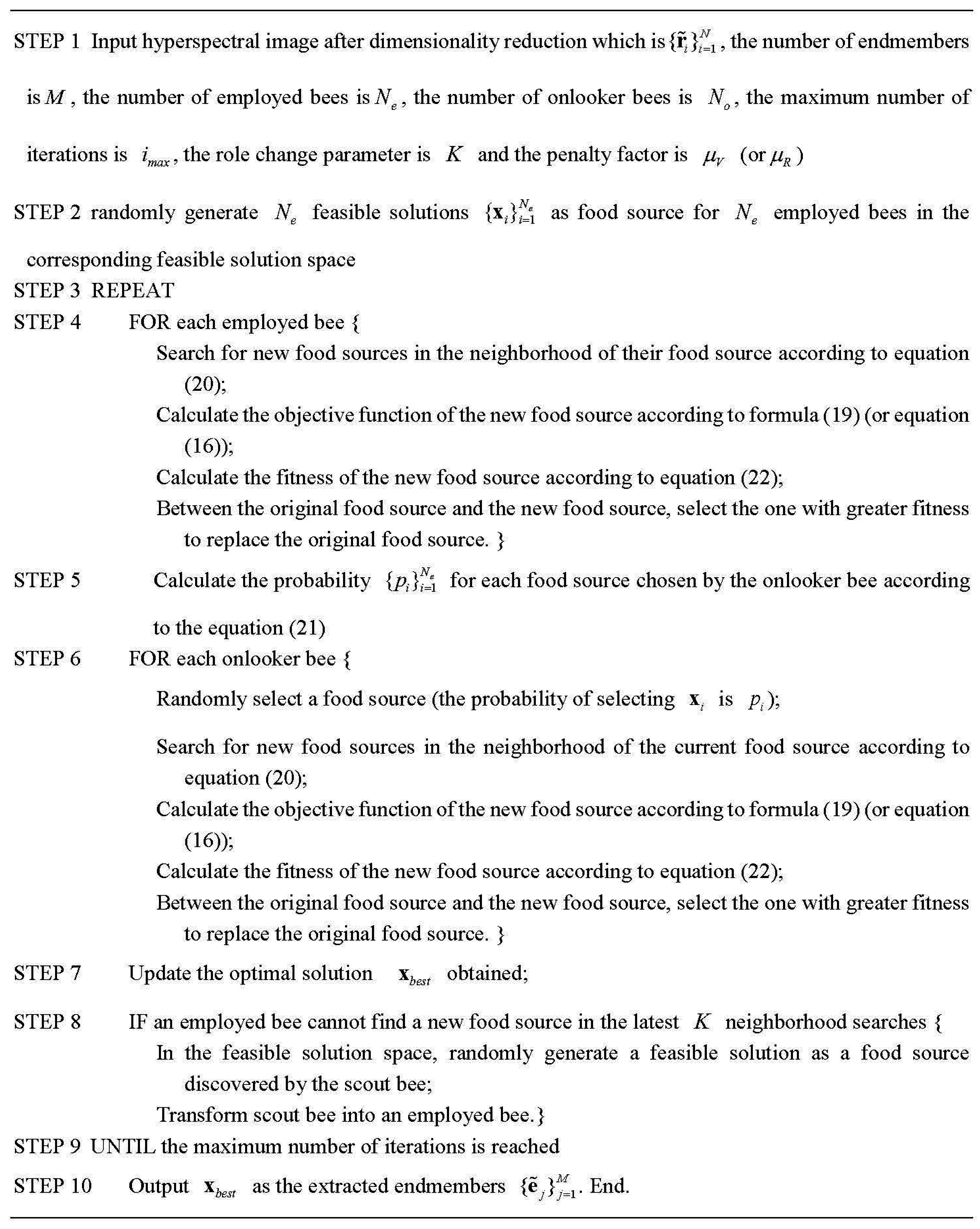
In this section, we discuss the use of three sets of synthetic data to evaluate the performance of ABCEE and present the results. The algorithms considered for comparison include ABCEE-R, ABCEE-V, AVMAX, MVC-NMF, MVSA, RMVES and VCA. These algorithms are all based on the LSMM and are the most typical ones among geometric-based approaches. AVMAX and VCA use model Equation (5). The difference between them is that VCA adopts the pure pixel assumption, which means that the endmember set is a subset of the pixels, whereas AVMAX does not require this assumption. MVSA and RMVES use model Equation (6), which is the closest model to that used in ABCEE. Although MVC-NMF uses NMF as the mathematical tool for endmember extraction and abundance inversion, its underlying principle can be regarded as an improvement to model Equation (6) through the use of the minimum-volume constraint.

The RMSE and spectral angle distance (SAD) were used to evaluate the results of the algorithms. The RMSE is defined as in Equation (18). The calculation of the RMSE requires no prior information. This measure can be obtained simply from the hyperspectral image and extracted endmembers. It indicates how much information is lost in endmember extraction. A smaller RMSE value implies higher quality endmembers. The SAD is defined as

$$SAD(a,b)=\arccos \left(\frac{a^{T}b}{\left|\right|a\left|\right|\cdot \left|\right|b\left|\right|}\right)$$

(23)

where $a$ and $b$ are two spectra. The calculation of the SAD requires another spectral library to compare with the extracted endmembers. This measure indicates the similarity between the endmembers and the materials in this spectral library. A smaller SAD value implies higher quality endmembers. However, it should be noted that the value of the SAD depends on not only the endmembers but also the spectral library.

According to [28], we set $K=2N_e$ and $N_e=N_o$ to reduce the number of parameters on the premise of assuring the algorithm’s effectiveness. Because any ABC algorithm has certain randomness, the results of each calculation are not exactly the same. To ensure the objective evaluation of the performance of ABCEE, each experiment involving ABCEE reported in this section was run 15 times, and the median of all 15 different outcomes of the objective function was considered to be the final result of the experiment.

3.1. Synthetic Dataset 1

The first synthetic dataset was generated using the following method. First, the spectra of five different materials (826 bands) were selected from the USGS Spectral Library to serve as the endmembers, denoted by ${\left\{e_j\right\}}_{j=1}^5$. Then, the abundances for each endmember were generated following [29]. For example, if the abundance of $e_1$ in the upper left point of the image is 1, then the abundance of this material progressively decreases to a minimum value of 0 for points increasingly far from that point; similarly, if the abundance of $e_5$ at the center is 1, then the abundance of this material also progressively decreases to a minimum value of 0 for points increasingly far from that point. Third, based on these abundances, the endmembers were mixed in accordance with the LSMM approach to obtain a synthetic image of 100 × 100 pixels. Finally, random noise with an SNR of 100:1 was added.

In practice, the exact number of endmembers in an image is typically unknown, and the number of endmembers estimated based on the image information may be greater or smaller than the true number of endmembers. Through experiments with different numbers of endmembers, this section presents an evaluation of the accuracy of endmember extraction when the number of endmembers is more than ($M=6$), equal to ($M=5$) or less than ($M=4$) the true number of endmembers; the results are shown in Table 1. As shown in the table, in cases of different numbers of endmembers, ABCEE-R achieves the best RMSE results.

For the case of $M=4$, the ABCEE-V RMSE is worse than that of ABCEE-R, but its volume is the smallest. For the case of $M=6$, although the RMVES volume, which is the best in this case, is slightly better than that of ABCEE-V, the ABCEE-V RMSE is vastly superior to that of RMVES. In other words, when the number of endmembers extracted is more or less than the true number of endmembers, ABCEE can produce good results, proving that an algorithm’s robustness can be enhanced by improving its objective function.

Table 1. Experimental results for synthetic hyperspectral dataset 1.

M	Index	AVMAX	MVCNMF	MVSA *	RMVES	VCA	ABCEE-R	ABCEE-V
4	RMSE	0.18621	0.084863	0.012774	0.087644	0.283535	0.011625	0.082551
	Volume	501.1301	359.0325	1799.304	710.6319	440.9159	777.213	320.0297
5	RMSE	0.004896	0.195454	0.009964	0.001838	0.007107	0.000681	0.003071
	Volume	1001.615	1055841	1253.954	1053.175	1001.296	2048.226	1537.273
	SAD (rad)	0.002236	0.081847	0.016715	0.004058	0.002254	0.051416	0.0868
6	RMSE	0.019094	0.472892	0.009954	0.221258	0.008665	0.004744	0.150269
	Volume	80.83104	60541510	827.5818	19.67032	61.82337	58.11748	21.25579

* The endmembers extracted via MVSA contained negative values; therefore the MVSA results were not compared with those of the other algorithms.

Table 1. Experimental results for synthetic hyperspectral dataset 1.

M	Index	AVMAX	MVCNMF	MVSA *	RMVES	VCA	ABCEE-R	ABCEE-V
4	RMSE	0.18621	0.084863	0.012774	0.087644	0.283535	0.011625	0.082551
	Volume	501.1301	359.0325	1799.304	710.6319	440.9159	777.213	320.0297
5	RMSE	0.004896	0.195454	0.009964	0.001838	0.007107	0.000681	0.003071
	Volume	1001.615	1055841	1253.954	1053.175	1001.296	2048.226	1537.273
	SAD (rad)	0.002236	0.081847	0.016715	0.004058	0.002254	0.051416	0.0868
6	RMSE	0.019094	0.472892	0.009954	0.221258	0.008665	0.004744	0.150269
	Volume	80.83104	60541510	827.5818	19.67032	61.82337	58.11748	21.25579

* The endmembers extracted via MVSA contained negative values; therefore the MVSA results were not compared with those of the other algorithms.

For the case of $M=5$, the RMSEs of both ABCEE algorithms are better than those of AVMAX, MVCNMF, MVSA and VCA, but their volumes are slightly worse. This is because the number of endmembers extracted equals to the true number of endmembers, and the pixels in the feature space truly exhibit the characteristics of a simplex after dimensionality reduction; moreover, the volumes calculated based on internal maximum-volume models (AVMAX and VCA) will obviously be smaller than the volumes calculated based on external minimum-volume models (the other four algorithms), and a larger volume means that more points are located inside the simplex, resulting in a smaller RMSE.

In addition, for the case of $M=5$, the SAD was considered to evaluate the differences between the extracted endmembers and the true endmembers; the results are shown in Table 1. As seen from the table, the SAD results of AVMAX and VCA (based on internal maximum-volume models) indicate the best performance, whereas the other five algorithms performed somewhat poorly. This is because the synthetic data contained pure pixels and a high SNR, conditions like that favor the internal maximum-volume approach. Among the five algorithms based on external minimum-volume models (excluding MVSA), the RMVES result is of the highest quality, followed by the ABCEE-R result, whereas the endmembers extracted via ABCEE-V deviate the most from the true endmembers; these findings are consistent with the design of ABCEE-V, whose objective function attempts to achieve a tradeoff between volume and error.

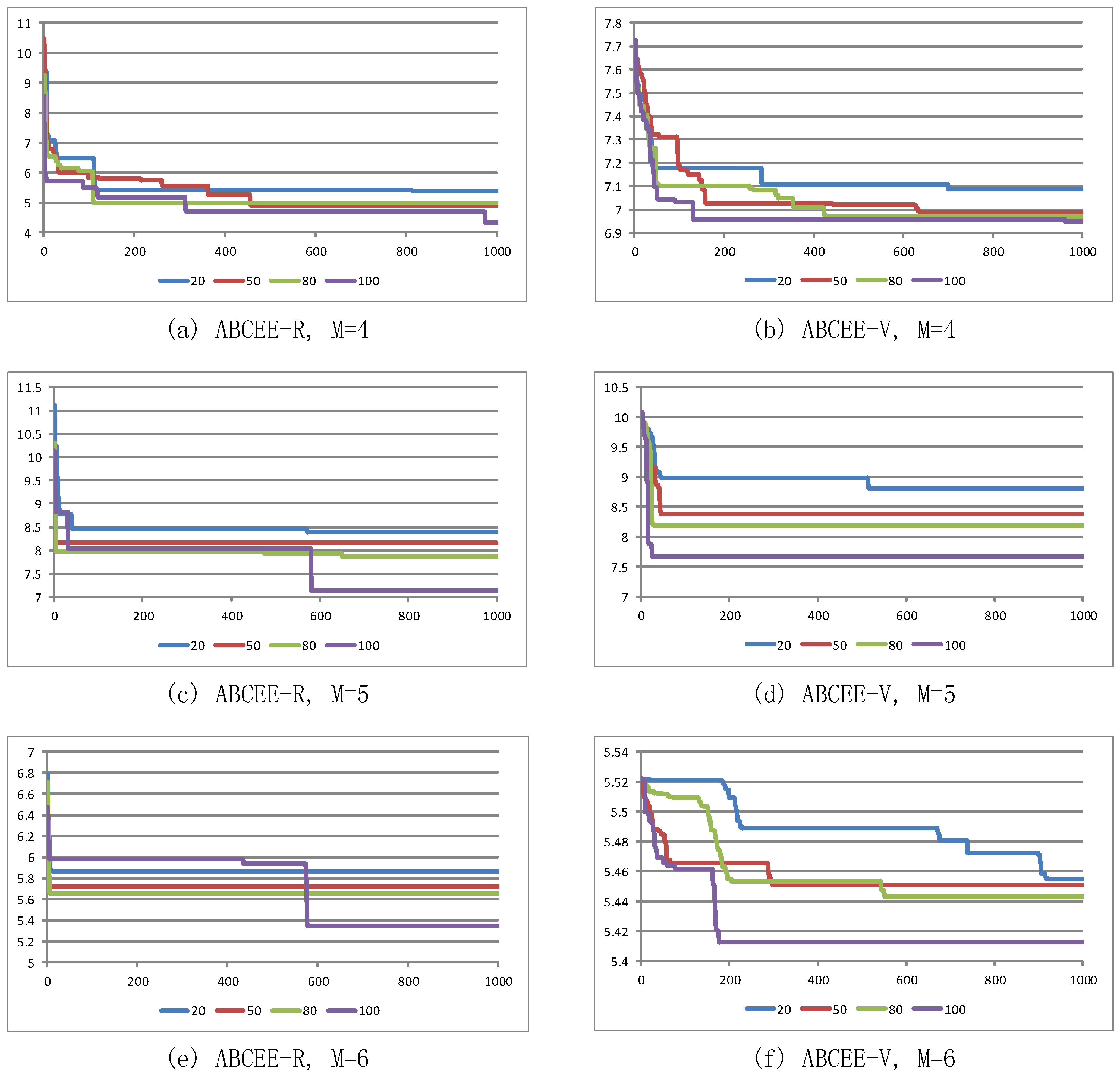
The objective function values of the different iterations of ABCEE algorithms are shown in Figure 3, where the horizontal axis represents the number of iterations, the vertical axis represents the logarithm of the objective function, and the colors represent the colony size, which is the sum of the numbers of employed and onlooker bees (i.e., $N_e+N_o$). For the experiments presented in this paper, these numbers were set to be identical (i.e., $N_e=N_o$). It is evident from the figure that significant changes in the objective function values occur over the first 200 iterations. This is because the quality of the randomly generated initial solutions is poor and has a large potential for optimization, giving rise to a high optimization speed. As the number of iterations increases, the optimization speed is reduced, and in most cases, after 600 iterations, the objective function may be difficult to optimize further. The computation times for different colony sizes are shown in Table 2. As indicated in Figure 3 and Table 2, a larger colony size yields a better final objective function value but also leads to longer computation time. This is because with a greater colony size, the number of search neighborhoods increases, and a better solution is more likely to be found. The computation time for each neighborhood search is nearly identical; therefore, the colony size (i.e., the number of searches) directly determines the total computation time.

Table 2. ABCEE computation time comparison for different populations (seconds).

Algorithm		Population	20	50	80	100
	Number of Endmembers
ABCEE-R	4		630.94	1540.09	2475.27	3070.64
	5		680.75	1718.50	4117.73	3433.15
	6		733.81	1728.14	2751.05	3424.61
ABCEE-V	4		24.84	62.73	98.05	125.10
	5		32.78	80.20	144.30	189.03
	6		33.51	83.11	132.93	169.73

Table 2. ABCEE computation time comparison for different populations (seconds).

Algorithm		Population	20	50	80	100
	Number of Endmembers
ABCEE-R	4		630.94	1540.09	2475.27	3070.64
	5		680.75	1718.50	4117.73	3433.15
	6		733.81	1728.14	2751.05	3424.61
ABCEE-V	4		24.84	62.73	98.05	125.10
	5		32.78	80.20	144.30	189.03
	6		33.51	83.11	132.93	169.73

Figure 3. Changes in the ABCEE objective function over the course of multiple iterations. The horizontal axis represents the iteration number, and the vertical axis represents the logarithm of the objective function value. (a) ABCEE-R, M=4; (b) ABCEE-V, M=4; (c) ABCEE-R, M=5; (d) ABCEE-V, M=5; (e) ABCEE-R, M=6; (f) ABCEE-V, M=6.

Figure 3. Changes in the ABCEE objective function over the course of multiple iterations. The horizontal axis represents the iteration number, and the vertical axis represents the logarithm of the objective function value. (a) ABCEE-R, M=4; (b) ABCEE-V, M=4; (c) ABCEE-R, M=5; (d) ABCEE-V, M=5; (e) ABCEE-R, M=6; (f) ABCEE-V, M=6.

In this experiment, nine values of ${\mu }_R$ and ${\mu }_V$ were considered to find the best value of penalty factor, respectively. We set ${\mu }_{R,V}={10}^n,n_0-4\le n\le n_0+4$ here, where $n_0$ is the order-of-magnitude difference between the two parts of the objective function, and its value can be determined by an initial endmember extraction result obtained by any kind of algorithms of short computing time, such as AVMAX and VCA, without considering the pure pixel assumption. While $M=5$, $n_0$ was set to 5 for ${\mu }_R$ and 3 for ${\mu }_V$.

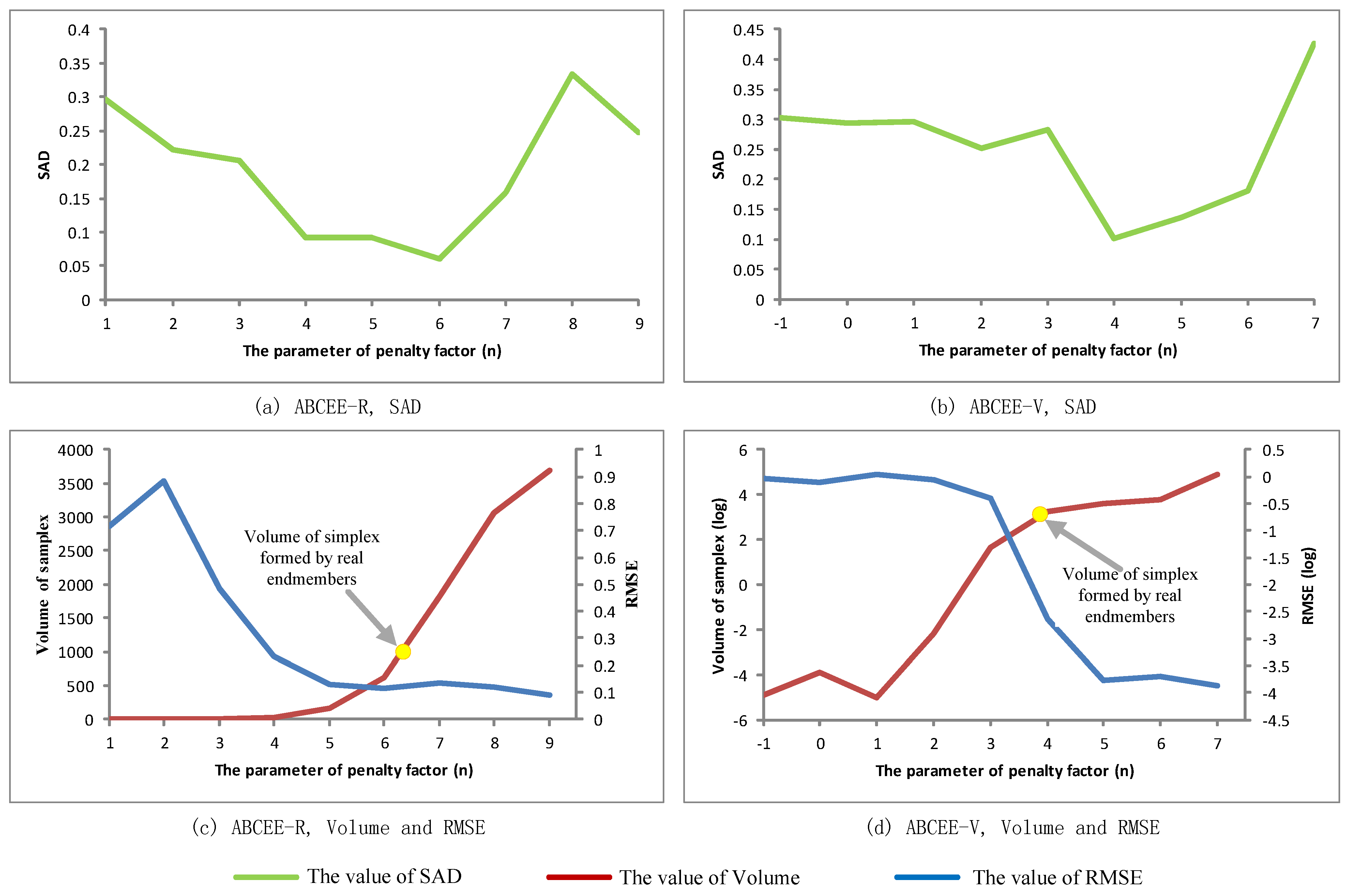
Figure 4 reflects the influence of the penalty factors ${\mu }_R$ and ${\mu }_V$ on the endmember extraction results. The horizontal axis represents the corresponding value of $n$ for each penalty factor. The average SAD, the volume of the simplex and the RMSE were used as indicators for evaluating ${\mu }_R$ and ${\mu }_V$. It is apparent from Figure 4a,b that for both ${\mu }_R$ and ${\mu }_V$, the results are optimal when $n=n_0+1$. Besides, from Figure 4c,d, it can be found that the simplex’s volume of extracted endmembers is most similar to that of real endmembers while $n=n_0+1$, which is consistent of the results of SAD. If $n<n_0$, the proportion of volume in all the factors contained in objective function is too large, which results to the very small value of simplex volume, the very large values of RMSE and SAD. Obviously, this kind of result is not right. On the other hand, if $n>n_0+1$, the proportion of volume in all the factors contained in objective function is too small, which means that with the increase of $n$, the algorithm is more likely to find the solutions of smaller RMSE, even though the simplex volume may become bigger or few points may not contained in the simplex. Actually, if a simplex volume is big enough, all pixels are contained in the simplex, so it is extremely hard to optimize RMSE, which can be proved by the experiments shown in Figure 4c,d that RMSE varied little while enlarging its volume.

Figure 4. Influence of the penalty factors ${\mu }_R$ and ${\mu }_V$ (a) the SAD of ABCEE-R; (b) the SAD of ABCEE-V; (c) the Volume and RMSE of ABCEE-R; (d) the Volume and RMSE of ABCEE-V.

Figure 4. Influence of the penalty factors ${\mu }_R$ and ${\mu }_V$ (a) the SAD of ABCEE-R; (b) the SAD of ABCEE-V; (c) the Volume and RMSE of ABCEE-R; (d) the Volume and RMSE of ABCEE-V.

Based on the analysis above, it is known that the value setting of ${\mu }_R$ and ${\mu }_V$ plays a crucial role in the final result of endmember extraction. In addition, we can conclude that while $n=n_0+1$, a result of the best tradeoff between Volume and RMSE can be obtained. Therefore, in this paper, the value of ${\mu }_R$ and ${\mu }_V$ in other experiments can be defined by the following steps, (1) extract a set of initial endmembers using AVMAX, (2) calculate its corresponding volume, penalty term (RMSE in Equation (19) or the number of points outside simplex in Equation (16)) and the ratio $\omega$, and (3) calculate ${\mu }_R$ and ${\mu }_V$ according the following formula.

$${\mu }_{V,R}=\left[\frac{\omega }{{10}^{[\lg \omega ]-1}}\right]\cdot {10}^{[\lg \omega ]}$$

(24)

3.2. Synthetic Dataset 2

The second synthetic dataset included 16 data calculated with four different numbers of endmembers (m = 4, 8, 16 and 20) and four different SNRs (90:1, 70:1, 50:1 and 30:1). All endmembers were drawn from the USGS Spectral Library, and the abundance of each endmember in each pixel, following beta distributions, was generated in accordance with [6]. Once the endmembers and abundances were prepared, they were multiplied together and summed to constitute the first term of Equation (1), and then, Gaussian white noise spectra with different SNRs were added in.

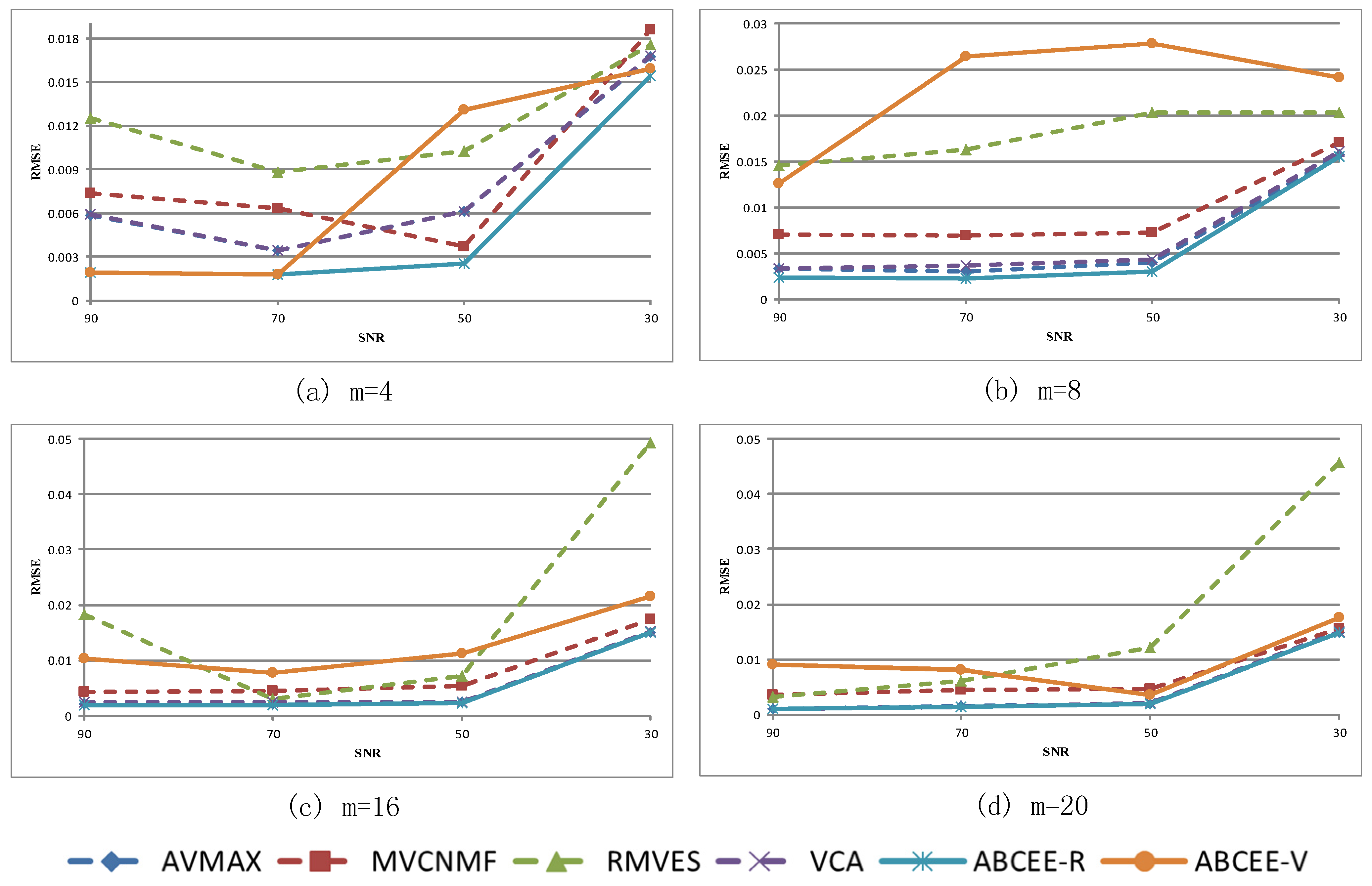
The RMSEs of the 16 data in synthetic Dataset 1 are shown in Figure 5. The RMSEs for MVSA are not contained in this figure because the endmembers extracted via MVSA contain negative values, which is clearly unreasonable. The reason for this phenomenon is that MVSA is based on an external minimum-volume model, and its calculation using Sequential Quadratic Programming (SQP), but its feasible solution space is not constrained to be non-negative. The core algorithm of MVC-NMF is non-negative matrix factorization and thus contains a non-negative constraint, and ABCEE’s feasible solution space is also subject to a non-negative constraint; therefore, the three corresponding algorithms, though also based on the minimum-volume approach, do not produce results that contain negative values.

Figure 5. RMSEs for synthetic Dataset 2. (a) m=4; (b) m=8; (c) m=16; (d) m=20.

Figure 5. RMSEs for synthetic Dataset 2. (a) m=4; (b) m=8; (c) m=16; (d) m=20.

Figure 5 demonstrates that ABCEE-R is clearly superior to the other algorithms when the number of endmembers is relatively small (m = 4 or 8), whereas in other circumstances (m = 16 or 20), the performances of ABCEE-R, AVMAX and VCA are nearly identical. Among these 16 experiments, ABCEE-R achieved the smallest RMSE 12 times, whereas ABCEE-V and VCA achieved the smallest RMSE two times each; in the latter cases, the RMSEs of ABCEE-R were ranked second, very close to the best results. Therefore, we can infer from these results that ABCEE-V is more suitable for experimental data with fewer endmembers and higher SNRs, whereas ABCEE-R is more robust. In addition, with a reduction in SNR, the RMSE values for each algorithm increase. However, ABCEE-R always retains its advantage over the other algorithms, illustrating its insensitivity to the number of endmembers and the SNR.

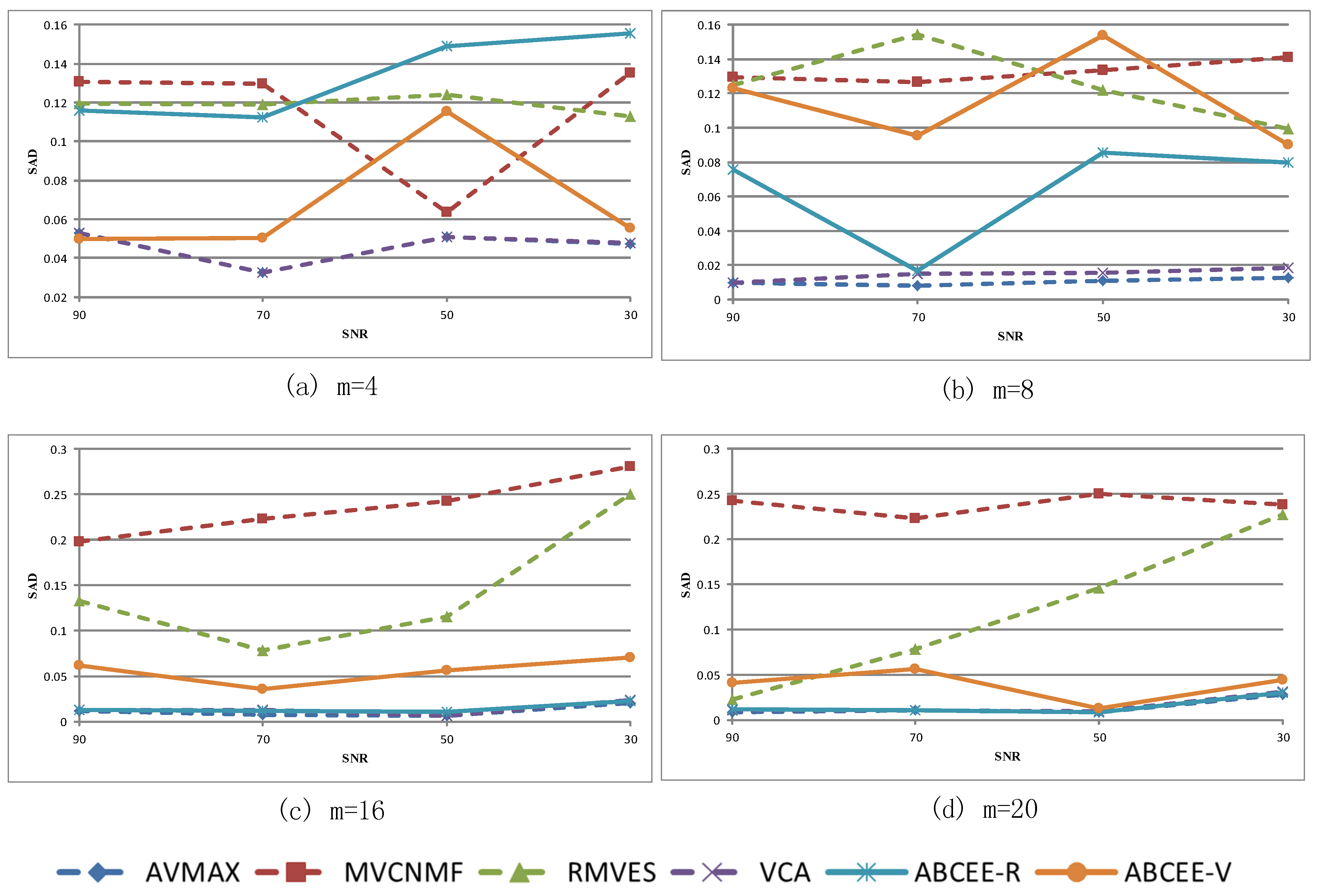
The SADs of the 16 data in synthetic Dataset 1 are shown in Figure 6. For the same reason discussed above, the results for MVSA were not added to this figure. No explicit trend is evident in the change of the SADs of the two ABCEE algorithms for the data with different SNRs. AVMAX and VCA can always obtain better SADs. This is because certain pixels can be very similar to certain endmembers when the abundances obey a beta distribution, which results in high proportions of certain endmembers in certain pixels. For example, for m = 4, these four endmembers’ maximum abundances were 0.9884, 0.9898, 0.9876 and 0.9887, indicating that in these simulated images, although noise was present, the pure pixel assumption was essentially satisfied. Therefore, any errors between the extracted endmembers and the real ones would predominantly originate from noise when an algorithm based on the internal maximum-volume method was used. The external minimum-volume method demonstrated no obvious advantages compared with the other methods, and because of the presence of noise, its endmember extraction results could be quite different from the real results when the endmembers were relatively few (m = 4 or 8). However, with an increasing number of endmembers (m = 16 or 20), the largest proportion of each endmember in a pixel gradually decreases; for example, for m = 20, the smallest value among the maximum abundances of these 20 endmembers was merely 0.8784. Therefore, under these circumstances, the SAD of ABCEE-R gradually overtakes and eventually exceeds those of AVMAX and VCA. The results of ABCEE-V are also clearly superior those of MVC-NMF and RMVES, although they are inferior to those of ABCEE-R, especially when the SNR is low.

Figure 6. SADs for synthetic Dataset 2. (a) m=4; (b) m=8; (c) m=16; (d) m=20.

Figure 6. SADs for synthetic Dataset 2. (a) m=4; (b) m=8; (c) m=16; (d) m=20.

3.3. Synthetic Dataset 3

The third synthetic dataset is mixed by four endmembers, which are similar to the endmembers in the first synthetic dataset, while m = 4. The production process of this dataset is the same as the first synthetic dataset. It is noteworthy that the endmember abundance of the third synthetic dataset follows normal distribution, and each endmember’s maximum abundance in any pixel is no more than 80%. Besides, in the final step of adding Gaussian white noise, SNRs are 100:1 and 50:1, respectively. In general, this dataset simulates the circumstance that data contains no pure pixels.

The results are shown in Table 3. It can be seen that for the circumstances of two different SNRs, ABCEE-R and ABCEE-V can always obtain the minimum RMSE and SAD, respectively, which means that ABCEE can gain better endmember extraction results no matter how high or how low the SNR is while processing images without pure pixels. The experiment results are coordinated with the purpose of ABCEE’s objective function design. Equation (19) assures the volume of simplex can be well maintained while optimizing RMSE, which makes the spectral angle of the extracted and real endmembers be maintained in a suitable ranges (better than MCV-NMF and RMVES) while getting the minimum RMSE using ABCEE-R. Besides, Equation (16) allows few data points located in the outside of simplex while searching the external minimum-volume, which brings the endmembers extracted by ABCEE-V closer to real endmembers, and its RMSE only inferior to ABCEE-R and MVSA.

Table 3. Experimental results for synthetic hyperspectral dataset 3.

SNR	Metric	AVMAX	MVC-NMF	MVSA	RMVES	VCA	ABCEE-R	ABCEE-V
100:1	SAD	0.12444	0.174573	0.057896	0.208851	0.124838	0.149328	0.040319
	RMSE	0.028656	0.076074	1.18 × 10−16	0.261966	0.034615	1.02 × 10−16	0.003675
50:1	SAD	0.120362	0.177811	0.08611	0.153927	0.118427	0.145519	0.049782
	RMSE	0.023661	0.078122	1.35 × 10−16	0.006434	0.0319	1.02 × 10−16	0.006023

Table 3. Experimental results for synthetic hyperspectral dataset 3.

SNR	Metric	AVMAX	MVC-NMF	MVSA	RMVES	VCA	ABCEE-R	ABCEE-V
100:1	SAD	0.12444	0.174573	0.057896	0.208851	0.124838	0.149328	0.040319
	RMSE	0.028656	0.076074	1.18 × 10−16	0.261966	0.034615	1.02 × 10−16	0.003675
50:1	SAD	0.120362	0.177811	0.08611	0.153927	0.118427	0.145519	0.049782
	RMSE	0.023661	0.078122	1.35 × 10−16	0.006434	0.0319	1.02 × 10−16	0.006023

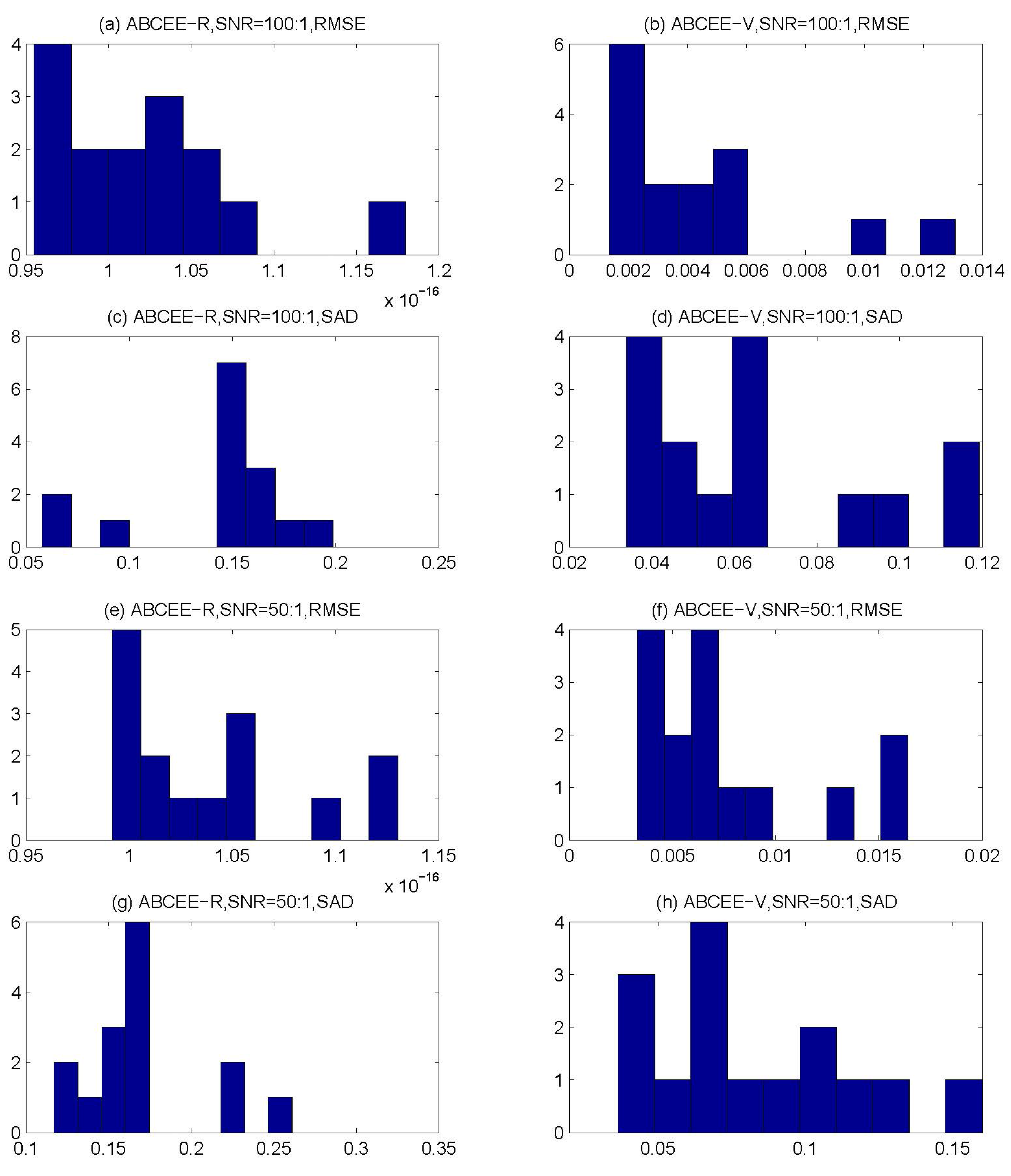
Besides, the synthetic dataset 3 is also used to evaluate the robustness of ABCEE. Table 4 represents the SAD and RMSE’s average value and standard deviation of ABCEE-R and ABCEE-V’s results by computing 15 times. Figure 7 shows the histogram of these results. From Table 4, it can be seen that the standard deviations of ABCEE are always smaller than 0.05, which shows the stabilization of the algorithm, even though the endmember extraction results are different. In addition, from the point view of relative value of standard deviation and average value, the robustness of ABCEE-R is better than ABCEE-V.

On another hand, we can see from Figure 7 that most results are concentrated in a small interval under the same circumstances and only very few results are abnormal, such as the result at the far right in Figure 7a, and the two results at the far right in Figure 7b. It can be found that in 120 results, only 20 results are abnormal, which means that 83.33% results can be located in a good interval by ABCEE.

Table 4. The mean and standard deviation of 15 times run of ABCEE.

		ABCEE-R		ABCEE-V
		RMSE	SAD	RMSE	SAD
SNR = 100:1	Mean	1.02 × 10−16	0.143641	0.004334	0.064347
	Stdev	5.79 × 10−18	0.040741	0.003203	0.026924
SNR = 50:1	Mean	1.04 × 10−16	0.1681471	0.007672	0.082615
	Stdev	4.57 × 10−18	0.0380169	0.004312	0.035142

Table 4. The mean and standard deviation of 15 times run of ABCEE.

		ABCEE-R		ABCEE-V
		RMSE	SAD	RMSE	SAD
SNR = 100:1	Mean	1.02 × 10−16	0.143641	0.004334	0.064347
	Stdev	5.79 × 10−18	0.040741	0.003203	0.026924
SNR = 50:1	Mean	1.04 × 10−16	0.1681471	0.007672	0.082615
	Stdev	4.57 × 10−18	0.0380169	0.004312	0.035142

Figure 7. Hist of the synthetic Dataset 3. (a) ABCEE-R, SNR=100:1, RMSE; (b) ABCEE-V, SNR=100:1, RMSE; (c) ABCEE-R, SNR=100:1, SAD; (d) ABCEE-V, SNR=100:1, SAD; (e) ABCEE-R, SNR=50:1, RMSE; (f) ABCEE-V, SNR=50:1, RMSE; (g) ABCEE-R, SNR=50:1, SAD; (h) ABCEE-V, SNR=50:1, SAD.

Figure 7. Hist of the synthetic Dataset 3. (a) ABCEE-R, SNR=100:1, RMSE; (b) ABCEE-V, SNR=100:1, RMSE; (c) ABCEE-R, SNR=100:1, SAD; (d) ABCEE-V, SNR=100:1, SAD; (e) ABCEE-R, SNR=50:1, RMSE; (f) ABCEE-V, SNR=50:1, RMSE; (g) ABCEE-R, SNR=50:1, SAD; (h) ABCEE-V, SNR=50:1, SAD.

4. Experiments with a Real Image

In this section, we present the application of ABCEE-R and ABCEE-V for endmember extraction from a hyperspectral image of Cuprite, Nevada, which was collected by the Airborne Visible/Infrared Imaging Spectrometer (AVIRIS) and provided by ENVI. This data is widely used in research on hyperspectral image processing algorithms, such as spectral unmixing and classification, and a highly accurate ground truth is available for testing the results of such algorithms. The original AVIRIS data contain 224 channels, with a spectral resolution of 10 nm, wavelength ranges between 400 and 2500 nm, and a spatial resolution of 20 m. The AVIRIS data provided by ENVI contain only 50 bands ranging from 1990.8 to 2479 nm, and the image size is 400 × 350 pixels. Because one of the predominant materials present in the region is salt and the provided wavelength range (1990.8–2479 nm) enables adequately distinction of the typical salt mines in the region, this ENVI data was used in this study to test endmember extraction and abundance inversion. As in Section 3, the experiments presented in this section were also performed using AVMAX, MVSA, RMVES, MVC-NMF and VCA for comparison. According to the HySime algorithm, the number of endmembers to be extracted was 8. The parameters of the ABCEE algorithms were set as follows: $N_e=N_o=25$ and $i_{max}=200$. A set of initial endmembers is generated by AVMAX, whose volume and RMSE are shown in Table 5. According to Equation (24), the penalty factors for the Cuprite data are ${\mu }_V=2.5E+17$ and ${\mu }_R=1.0E+17$.

Table 5. Results for Cuprite data.

	AVMAX	MVC-NMF	MVSA	RMVES	VCA	ABCEE-R	ABCEE-V
RMSE (FCLS)	5.968194	12.29701	2.585935	7.86 × 10−3	8.583891	2.3984 × 10−4	3.44976
VOLUME	5.30 × 1016	37,133.88	4.59 × 1020	1.83 × 1019	2.78 × 1016	2.04 × 1012	1.30 × 1017

Table 5. Results for Cuprite data.

	AVMAX	MVC-NMF	MVSA	RMVES	VCA	ABCEE-R	ABCEE-V
RMSE (FCLS)	5.968194	12.29701	2.585935	7.86 × 10−3	8.583891	2.3984 × 10−4	3.44976
VOLUME	5.30 × 1016	37,133.88	4.59 × 1020	1.83 × 1019	2.78 × 1016	2.04 × 1012	1.30 × 1017

The RMSEs obtained via the FCLS approach using the endmembers extracted by the algorithms and the volumes of the simplexes formed by those endmembers are shown in Table 5. It is evident from Table 5 that ABCEE-R yielded the smallest RMSE. Although the MVC-NMF volume is smaller than that of ABCEE-R, its RMSE is much worse than that of ABCEE-R—in fact, it is the worst among all the tested algorithms. Thus, the ABCEE-R result can be considered to be the best.

According to the Cuprite ground truth provided by the USGS, the major minerals in this region include alunite, buddingtonite, calcite, chalcedony, chlorite, dickite, jarosite, kaolinite, montmorillonite, muscovite, and nontronite. The image area also contains these minerals. The SADs were calculated between the standard spectra of these minerals from the USGS Mineral Spectral Library and the endmembers extracted by the algorithms. For each endmember, the mineral with the smallest corresponding SAD was selected as the mineral associated with the endmember. The performances of the algorithms were compared in terms of the number, type and average spectral angle of each mineral. The results are shown in Table 6 and Figure 8.

As seen from the results, the minerals corresponding to several of the extracted endmembers were duplicates (e.g., AVMAX extracted two chalcedony and two montmorillonite endmembers), and the minerals extracted by the various algorithms were not the same. In terms of quantity, ABCEE-R extracted seven different minerals, and the other algorithms each extracted six different minerals. From the types of minerals extracted, we conclude that most algorithms can extract five minerals—alunite, chalcedony, kaolinite, montmorillonite and nontronite. A comparison with the ground truth reveals that the image region indeed contains large amounts of these five types of minerals; however, MVC-NMF failed to correctly extract alunite, MVSA failed to correctly extract kaolinite, and RMVES missed montmorillonite. From the perspective of the average spectral angle, those of AVMAX, VCA and ABCEE-V were less than 0.1, indicating that the extracted endmembers were very close to the true minerals, because the distinction among minerals in Cuprite is obvious and the hyperspectral image of this region can be considered to contain pure pixels of various minerals. Therefore, AVMAX and VCA, which are based on internal maximum-volume models, yielded the best SADs. Meanwhile, although based on an external minimum-volume model, ABCEE-V does not require the simplex formed by the endmembers to completely contain the convex hull formed by the pixels; this enhances the algorithm’s robustness and allows it to produce a better endmember extraction result.

Figure 9 and Figure 10 show the FCLS results for the endmembers extracted by ABCEE-R and ABCEE-V, respectively. Obviously, the abundance estimation results for alunite (Figure 9e and Figure 10g), kaolinite (Figure 9f and Figure 10f) and chalcedony (Figure 9c and Figure 10a), which are common in Cuprite, that were obtained using these two methods are found to be similar. For nontronite, ABCEE-R produced better estimation results than did ABCEE-V because two different nontronite endmembers were extracted using ABCEE-V, directly resulting in a larger RMSE for ABCEE-V. In addition, no endmember corresponding to the typical mineral dickite was effectively extracted by ABCEE-V, which is another major reason for the superior performance of ABCEE-R.

Table 6. SADs between the endmembers extracted using the different algorithms and the corresponding spectra in USGS Spectral Library.

	AVMAX	MVCNMF	MVSA	RMVES	VCA	ABCEE-R	ABCEE-V
Alunite	0.075778		0.162828	0.330214	0.077421	0.330027	0.07927
Buddingtonite			0.163507	0.52489		0.543818
Buddingtonite			0.799628	0.111666		0.10611
Calcite		0.107456
Chalcedony	0.077258	0.077634	0.064867	0.096033	0.065664	0.115396	0.077258
Chalcedony	0.074673			0.073837	0.077258		0.08569
Chlorite	0.108636		0.195042
Dickite			0.637588	0.301254		0.427711
Dickite			2.814941
Jarosite		0.136408
Kaolinite	0.072725	0.150208		0.163789	0.063718	0.149905	0.073869
Kaolinite		0.110306
Montmorillonite	0.090629	0.097323	0.288801		0.090655	0.053652	0.098983
Montmorillonite	0.090655	0.074053			0.0671
Muscovite					0.094221		0.105594
Nontronite	0.086577	0.165434		0.300711	0.121372	0.373013	0.092121
Nontronite							0.097562
Average	0.084616	0.114853	0.6409	0.237799	0.082176	0.262454	0.088793

Table 6. SADs between the endmembers extracted using the different algorithms and the corresponding spectra in USGS Spectral Library.

	AVMAX	MVCNMF	MVSA	RMVES	VCA	ABCEE-R	ABCEE-V
Alunite	0.075778		0.162828	0.330214	0.077421	0.330027	0.07927
Buddingtonite			0.163507	0.52489		0.543818
Buddingtonite			0.799628	0.111666		0.10611
Calcite		0.107456
Chalcedony	0.077258	0.077634	0.064867	0.096033	0.065664	0.115396	0.077258
Chalcedony	0.074673			0.073837	0.077258		0.08569
Chlorite	0.108636		0.195042
Dickite			0.637588	0.301254		0.427711
Dickite			2.814941
Jarosite		0.136408
Kaolinite	0.072725	0.150208		0.163789	0.063718	0.149905	0.073869
Kaolinite		0.110306
Montmorillonite	0.090629	0.097323	0.288801		0.090655	0.053652	0.098983
Montmorillonite	0.090655	0.074053			0.0671
Muscovite					0.094221		0.105594
Nontronite	0.086577	0.165434		0.300711	0.121372	0.373013	0.092121
Nontronite							0.097562
Average	0.084616	0.114853	0.6409	0.237799	0.082176	0.262454	0.088793

Figure 8. Endmember extraction curve for each algorithm.

Figure 8. Endmember extraction curve for each algorithm.

Figure 9. ABCEE-R abundance inversion results for the Cuprite data. (a) Nontronite; (b) Buddingtonite; (c) Chalcedony; (d) Dickite; (e) Alunite; (f) Kaolinite; (g) Buddingtonite; (h) Montmorillonit.

Figure 9. ABCEE-R abundance inversion results for the Cuprite data. (a) Nontronite; (b) Buddingtonite; (c) Chalcedony; (d) Dickite; (e) Alunite; (f) Kaolinite; (g) Buddingtonite; (h) Montmorillonit.

Figure 10. ABCEE-V abundance inversion results for the Cuprite data. (a) Chalcedony; (b) Nontronite; (c) Nontronite; (d) Montmorillonit; (e) Chalcedony; (f) Kaolinite; (g) Alunite; (h) Muscovite.

Figure 10. ABCEE-V abundance inversion results for the Cuprite data. (a) Chalcedony; (b) Nontronite; (c) Nontronite; (d) Montmorillonit; (e) Chalcedony; (f) Kaolinite; (g) Alunite; (h) Muscovite.

5. Conclusions

The results of endmember extraction directly affect the reliability and accuracy of hyperspectral image spectral unmixing. Based on an external minimum-volume model as well as improvements to the objective function and the construction of the feasible solution space, this paper proposed two ABC-based endmember extraction algorithms: ABCEE-R and ABCEE-V. These algorithms combine the advantages of the improved model and the intelligent algorithm, and both achieve a suitable balance between volume and accuracy, thereby improving the robustness of the results and the ability to search for better endmembers in a continuous feasible solution space without requiring the pure pixel assumption. Besides, parameters of these algorithms have been carefully analyzed, especially, based on the analysis, an estimation method of penalty factor has been given, by which, a result of good tradeoff between the simplex volume and RMSE can be obtained.

Experiments have been carried out to prove the proposed algorithms’ performance and the following conclusions can be made. (1) If there are pure pixels, namely the biggest abundance equals to 1, the results of ABCEE is very similar to the best results obtained by the state-of-the-art methods, especially ABCEE-R can yield the best RMSE no matter the number of endmembers extracted is more than, less than or equal to the true number of endmembers or not; (2) If there are no pure pixels, namely the biggest abundance is smaller than 0.8, the results of ABCEE is better than the results obtained by the state-of-the-art methods; (3) If the number of endmember is relatively large, ABCEE can obtain the similar results under conditions of different SNR. Based on these conclusions, we can infer that the proposed algorithms own unique advantages while extracting endmember using hyperspectral images of low spatial resolution, complex ground objects and uncertain endmember quantity.

Besides, research on the use of swarm intelligence algorithms for endmember extraction is still in its infancy. There are many important aspects of the problem that should be further explored. For example, the common disadvantage of all swarm intelligence algorithms, including ABC, is their low calculation speed. Therefore, the use of parallel processing and other means to improve computational efficiency should be a major focus of future research.

References

1. Keshava, N.; Mustard, J.F. Spectral unmixing. IEEE Signal Process. Mag. 2002, 19, 44–57. [Google Scholar] [CrossRef]
2. Plaza, A.; Martin, G.; Plaza, J. Recent developments in endmember extraction and spectral unmixing. In Optical Remote Sensing; Springer: Berlin, Germany, 2010; pp. 235–267. [Google Scholar]
3. Bioucas-Dias, J.M.; Plaza, A.; Dobigeon, N. Hyperspectral unmixing overview: Geometrical, statistical, and sparse regression-based approaches. IEEE J. Sel. Top. Appl. Earth Observ. Remote Sens. 2012, 5, 354–379. [Google Scholar] [CrossRef]
4. Boardman, J.W.; Kruse, F.A.; Green, R.O. Mapping target signatures via partial unmixing of aviris data. In Proceedings of the Fifth Annual JPL Airborne Earth Science Workshop, Pasadena, California, 23–26 January 1995.
5. Winter, M.E. N-Findr: An algorithm for fast autonomous spectral end-member determination in hyperspectral data. SPIE Proc. 1999, 3753, 266–275. [Google Scholar]
6. Nascimento, J.M.; Dias, J.M. Vertex Component analysis: A fast algorithm to unmix hyperspectral data. IEEE Trans. Geosci. Remote Sens. 2005, 43, 898–910. [Google Scholar] [CrossRef]
7. Chang, C.; Wu, C.; Liu, W. A new growing method for simplex-based endmember extraction algorithm. IEEE Trans. Geosci. Remote Sens. 2006, 44, 2804–2819. [Google Scholar] [CrossRef]
8. Gruninger, J.H.; Ratkowski, A.J.; Hoke, M.L. The sequential maximum angle convex cone (smacc) endmember model. Proc Spie 2004, 5425, 1–14. [Google Scholar]
9. Chan, T.; Ma, W.; Ambikapathi, A. A simplex volume maximization framework for hyperspectral endmember extraction. IEEE Trans. Geosci. Remote Sens. 2011, 49, 4177–4193. [Google Scholar] [CrossRef]
10. Jun, L.; José, M.B. Minimum volume simplex analysis: A fast algorithm to unmix hyperspectral data. IEEE Trans. Geosci. Remote Sens. 2008, 3, 250–253. [Google Scholar]
11. Ambikapathi, A.; Chan, T.; Ma, W. Chance-constrained robust minimum-volume enclosing simplex algorithm for hyperspectral unmixing. IEEE Trans. Geosci. Remote Sens. 2011, 49, 4194–4209. [Google Scholar] [CrossRef]
12. Miao, L.; Qi, H. Endmember extraction from highly mixed data using minimum volume constrained nonnegative matrix factorization. IEEE Trans. Geosci. Remote Sens. 2007, 45, 765–777. [Google Scholar] [CrossRef]
13. Dorigo, M.; Maniezzo, V.; Colorni, A. Ant system: Optimization by a colony of cooperating agents. IEEE Trans. Syst. Man Cybern. B Cybern. 1996, 26, 29–41. [Google Scholar] [CrossRef] [PubMed]
14. Eberhart, R.; Kennedy, J. A new optimizer using particle swarm theory. In Proceedings of the Sixth International Symposium on Micro Machine and Human Science, Nagoya, Japan, 4–6 October 1995.
15. Yang, X. Nature-Inspired Metaheuristic Algorithms; Luniver Press: Frome, UK, 2008. [Google Scholar]
16. Karaboga, D.; Basturk, B. A powerful and efficient algorithm for numerical function optimization: Artificial Bee Colony (ABC) algorithm. J. Glob. Optim. 2007, 39, 459–471. [Google Scholar] [CrossRef]
17. Zhang, B.; Sun, X.; Gao, L. Endmember extraction of hyperspectral remote sensing images based on the Ant Colony Optimization (ACO) algorithm. IEEE Trans Geosci. Remote Sens. 2011, 49, 2635–2646. [Google Scholar] [CrossRef]
18. Zhang, B.; Sun, X.; Gao, L. Endmember extraction of hyperspectral remote sensing images based on the discrete particle swarm optimization algorithm. IEEE Trans Geosci. Remote Sens. 2011, 49, 4173–4176. [Google Scholar] [CrossRef]
19. Karaboga, D.; Basturk, B. Artificial Bee Colony (ABC) optimization algorithm for solving constrained optimization problems. In Foundations of Fuzzy Logic and Soft Computing; Springer: Berlin, Germany, 2007; pp. 789–798. [Google Scholar]
20. Karaboga, D.; Akay, B.; Ozturk, C. Artificial Bee Colony (ABC) optimization algorithm for training feed-forward neural networks. In Modeling Decisions for Artificial Intelligence; Springer: Berlin, Germany, 2007; Volume 4617, pp. 318–329. [Google Scholar]
21. Baykasoglu, A.; Ozbakir, L.; Tapkan, P.I.N. Artificial Bee Colony algorithm and its application to generalized assignment problem. In Swarm Intelligence: Focus on Ant and Particle Swarm Optimization; Itech Education and Publishing: Vienna, Austria, 2007; pp. 113–144. [Google Scholar]
22. Wong, L.; Low, M.Y.H.; Chong, C.S. A Bee Colony Optimization algorithm for traveling salesman problem. In Proceedings of the Second Asia International Conference on Modelling & Simulation, Kuala Lumpur, Malaysia, 13–15 May 2008; pp. 818–823.
23. Karaboga, D.; Ozturk, C. A novel clustering approach: Artificial Bee Colony (ABC) algorithm. Appl. Soft Comput. 2011, 11, 652–657. [Google Scholar] [CrossRef]
24. Xiao, Y. Research on Bee Colony Algorithm and Its Applications in Image Processing. Ph.D. Thesis, South China University of Technology, Guangzhou, China, 2011. [Google Scholar]
25. Abu-Mouti, F.S.; El-Hawary, M.E. Overview of Artificial Bee Colony (ABC) algorithm and its applications. In Proceedings of the Systems Conference, Vancouver, BC, Canada, 19–22 March 2012; pp. 1–6.
26. Chang, C. Hyperspectral Data Exploitation: Theory and Applications; Wiley-Interscience: Hoboken, NJ, USA, 2007. [Google Scholar]
27. Heinz, D.C.; Chang, C. Fully constrained least squares linear spectral mixture analysis method for material quantification in hyperspectral imagery. IEEE Trans. Geosci. Remote Sens. 2001, 39, 529–545. [Google Scholar] [CrossRef]
28. Karaboga, D.; Basturk, B. On the Performance of Artificial Bee Colony (ABC) algorithm. Appl. Soft Comput. 2008, 8, 687–697. [Google Scholar] [CrossRef]
29. Plaza, A.; Martinez, P.; Perez, R. A quantitative and comparative analysis of endmember extraction algorithms from hyperspectral data. IEEE Trans. Geosci. Remote Sens. 2004, 42, 650–663. [Google Scholar] [CrossRef]