1. Introduction
Modern power distribution systems provide high service reliability. According to the US Department of Energy, today’s electricity system is 97.97% reliable [
1]. However, power outages and interruptions that can last for minutes to hours still occur. Power outages can be extremely expensive, costing the US Government $150 billion annually [
1]. Studies on 203 power cuts in the US revealed that the repair costs range from $500 to more than $140,000, comprising equipment replacement and repair [
2]. In addition to economic loss, power cuts have a negative impact on system reliability and customer satisfaction [
3]. Wildlife is the third leading-cause of power outages, after natural disasters and human-caused incidents, since electrical substations are constructed in open areas and can be easily reached by wildlife [
3]. This study is aimed at developing a solution to aid in the prevention of wildlife-related power outages.
Many different solutions have been proposed to prevent power outages. Burnham
et al. [
4] propose the use of cover-up materials and also suggest some modifications to the existing standard design of electrical substations such as pole-line reconfiguration. Sundararajan
et al. [
5] propose using perch guards, metal or plastic spikes and insulating caps to reduce bird-related outages. They also suggest constructing alternative perch sites close to substations to prevent birds from perching on transmission lines, in substations and on over-head distribution lines. Harness [
6] investigates which species come into contact with electrical equipment in different regions, and proposes covers, guards and reconfigurations specific to species causing power outages in a given region. The studies in [
4,
5,
6] do not address the issue with a comprehensive solution and they only focus on the prevention of bird-related power outages by proposing manual approaches. By applying modifications and insulations proposed in [
4,
5,
6], other sorts of wildlife, such as reptiles and mammals, can still cause power cuts.
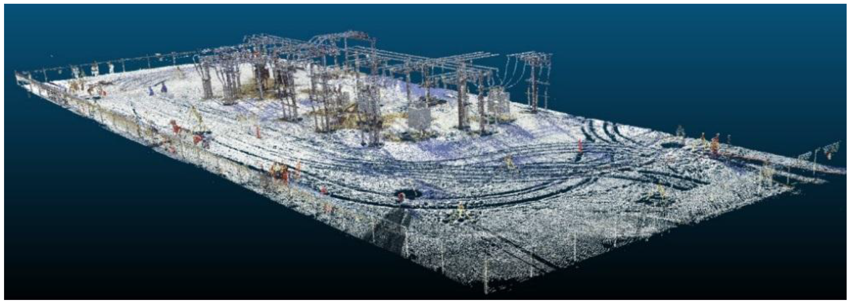
Covering the conductive elements of electrical substations with insulating materials can be a comprehensive solution to power outages caused by wildlife. Since the configuration of electrical substations can substantially differ from one to the next, non-conductive covers need to be custom-manufactured. The manufacture of the covers requires both an accurate inventory of substation components and accurate (centimeter-level) dimensions. In addition to site-to-site differences, the configuration and design of any given substations can change over time. Thus, any existing, as-designed plan is unlikely to be an accurate record of the current state of a site. Manual measurement of electrical equipment dimensions is not possible since safety restrictions require the substation to be de-energized, which is extremely costly. Technologies, such as laser scanning, offer safe and non-contact means of rapidly collecting substation data. Millions of three-dimensional (3D) data points can be measured within minutes. The key to exploiting these data for accurate dimensional characterization of substations is the automated recognition of relevant components from the data, which is the subject of this work.
2. Literature Review
To the best of authors’ knowledge, no comprehensive automated solution has been proposed to recognize all components of electrical substations from LiDAR data. Therefore, a review of studies that propose specific approaches for substation documentation using optical methods is first provided. This is followed by a review of methods for the segmentation and object recognition from LiDAR data in environments that share similarities with electrical substations. The similarities are in terms of the types of geometric primitives found on substation sites, i.e., linear, planar and cylindrical surfaces.
Although other studies have investigated the use of optical methods for substation documentation, they do so with manual methods or limit their scope to the recognition of specific components. Sternberg and Kersten [
7] manually construct a 3D model of an electrical substation by using commercial-available software. They approximate objects by simple geometric primitives,
i.e., electric power cables and insulators are represented by polylines and cylinders, respectively. Xu
et al. [
8] employ LiDAR data to study the current state of the electrical assets, such as power lines and electrical substations. However, they do not propose a systematic method for data processing and the inspection of electrical assets is carried out visually. Gonzalez-Aguilera
et al. [
9] employ digital camera images and photogrammetric techniques to model objects in electrical substations. Armeshi and Habib [
10] also recognize insulators of a substation site from digital images employing photogrammetric techniques. Photogrammetry can be restrictive in terms of the number of images that must be captured to completely cover a site and the close proximity to the electrical equipment at which they must be acquired, which may endanger the individual taking the images. Arastounia and Lichti [
11] recognize insulators from LiDAR data of a subset of an electrical substation point cloud. Both studies in [
10,
11] limit their scope to insulator recognition and other objects are not recognized. In this contribution, LiDAR data are collected by non-contact terrestrial laser scanners, which are able to scan the site from fewer instrument locations and from a farther distance compared to digital cameras. This significantly lowers the safety risks and duration of data collection. Noting that manual methods are used in [
7,
8], the aim of our contribution is to develop methods for automated recognition of electrical substations key components so that dimensions can be extracted in support of insulating cover manufacture.
Vosselman
et al. [
12] describe plane and cylinder recognition both by spatial-domain (surface growing) and parametric-domain (3D Hough transform that is an extension of Hough transform algorithm [
13]) algorithms. They recommend using spatial-domain methods for processing datasets larger than twenty million points. Belton and Lichti [
14] use local covariance analysis to segment smooth surfaces, edges and boundaries in an industrial site comprising planar and cylindrical surfaces. However, industrial objects are not individually recognized since they primarily focus on the segmentation. Rabbani
et al. [
15] propose a segmentation algorithm that uses a smoothness constraint to segment LiDAR data of industrial sites incorporating planar and cylindrical surfaces. The focus of this work is, however, limited to the segmentation of smoothly connected areas and objects in the site are not individually recognized. Pu and Vosselman [
16,
17,
18] extract building planar features, such as walls, roofs, and doors. First, planar surfaces are segmented and then some constraints, such as size, position, orientation, and point density are applied to recognize various features. Planar surfaces are segmented using a surface-growing algorithm, as explained in [
12]. Lehtomaki
et al. [
19] extract poles in a road environment using structured point clouds (scan lines). A scan line segmentation method is carried out based on proximity of points and the resulting segments are further analyzed to detect poles based on their size, shape and orientation. Martinez
et al. [
20] extract building facades in which planar surfaces are identified by RANSAC (RANdom Sample Consensus) [
21]. Arastounia and Lichti [
22] propose a new algorithm for plane segmentation, based on calculating the extent of points’ neighborhood in three cardinal directions and then compare it to principal components analysis (PCA). Although a LiDAR dataset of an electrical substation is used in this research, they only focus on the planar surface segmentation and no electrical equipment is recognized. Zhu
et al. [
23] reconstruct building 3D models using airborne laser scanner (ALS) data and topographic data in which planar surfaces (roof patches) are segmented by using PCA and eigenvalues analysis.
Much recent work has also focused on segmentation and recognition of linear features from LiDAR data. Melzer and Brieser [
24] introduce an algorithm for extracting power lines from ALS data in which the 2D Hough transform and RANSAC are employed to detect power line segments. This study assumes that power lines are parallel, which is not always the case. Jwa
et al. [
25] propose an algorithm to reconstruct power cables from a voxel-based, piece-wise line detector (VPLD). The entire dataset is divided into 3D voxels and both eigenvalue analysis and Hough transform are employed to detect linear neighborhoods. The results suffer from under- and over-segmentation, which are refined in [
26] by applying topological relationships among power cables. Sohn
et al. [
27] recognize power lines from ALS data using the method proposed in [
25]. However, they employ Markov Random Field (MRF) classifier to identify power lines from the linear segments based on segment height, slope and parallelism. Zhang
et al. [
28] classifies urban features such as ground, buildings and power lines from ALS data using support vector machine-based classification method. Zhu and Hyyppa [
29] extract power lines from ALS data. First, power line candidate points are identified by statistical analysis considering height, point density and histogram thresholds. Candidate points are then converted to 2D images and are further analyzed by image processing techniques. Zhu and Hyyppa [
30] model power lines in railroad environment from integrated ALS and MLS data. First, candidate power line points are identified based on some similarity measures,
i.e., points’ Z gradient with respect to their planimetric co-ordinates. Then, candidate points are converted to 2D images and image-processing techniques are employed to extract power lines. Cables appear as linear objects in both railroad corridors and electrical substation sites. However, railroad cables are usually much longer and their curvature is much less than that of electrical substations cables.
In our contribution, a new, fully-automated methodology is introduced to recognize key components of electrical substations. The proposed methodology is a data-driven approach that exploits unstructured LiDAR data containing only geometric information, i.e., only 3D co-ordinates of points. Furthermore, to improve the data processing efficiency, the data is processed in its original 3D point cloud format without converting it to 2D images or using image-processing techniques.
4. Methodology
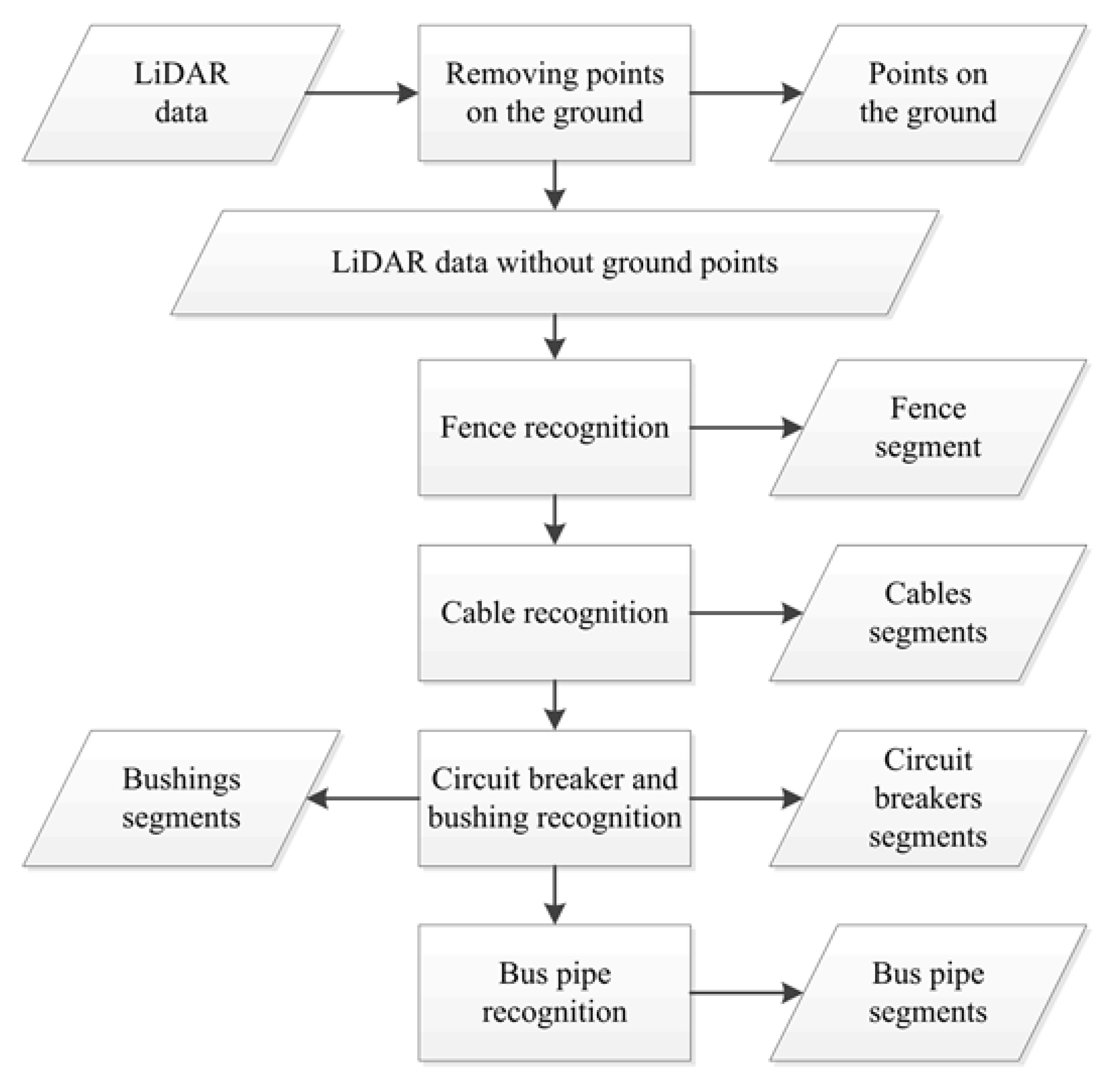
The methodology depicted in
Figure 2 is described in the following five subsections. In
Section 4.1, points on the ground are extracted and removed. Then, points belonging to the fence and cables are identified in the following two sections. The circuit breakers and bushings are recognized in
Section 4.4, which is followed by
Section 4.5 where points belonging to the bus pipes are recognized.
In many parts of the proposed methodology, local neighborhood statistics derived from PCA are used as cues. The basis of PCA is the construction and eigenvalue decomposition of the covariance matrix of 3D co-ordinates within each point’s neighborhood,
i.e.,
where:
A: square 3 × 3 covariance matrix of 3D co-ordinates within a point’s neighborhood;
λ: scalar eigenvalue;
V: 3 × 1 matrix representing an eigenvector (
).
Considering the dimensions of the covariance matrix (3 × 3), Equation (1) leads to three scalar eigenvalues (λ1, λ2, λ3 assuming λ1 ≥ λ2 ≥ λ3) and three eigenvectors (). Each eigenvalue (λi) represents the dispersion of a neighborhood in the direction of its corresponding eigenvector (). The eigenvalues and eigenvectors of the covariance matrix are used to infer local neighborhood structure.
Figure 2.
Flowchart of the entire methodology.
Figure 2.
Flowchart of the entire methodology.
4.1. Ground Removal
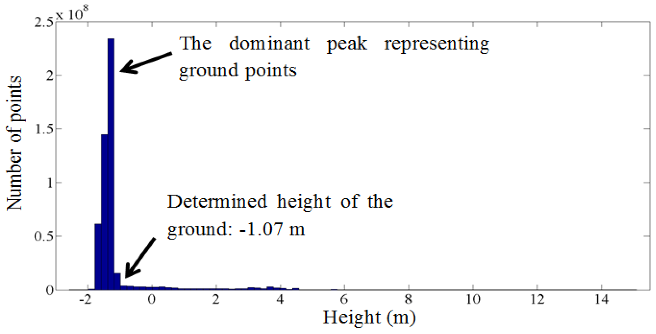
Although the ground within a substation site is not an important object, it needs to be removed since it usually constitutes a large proportion of total data volume. Substation sites typically have little topographical variation since they must be constructed on level ground. First, the height of the ground is determined from the height histogram of the entire point cloud. The dominant peak corresponding to points on the ground is automatically identified from which the ground height is determined. Points on or below the ground height are then easily discarded and the remaining points are retained for subsequent processing.
Figure 3 shows the height histogram of a sample dataset in which the upper arrow points to the dominant peak representing points on the ground and the lower arrow points to the determined height of the ground. The bin width must large enough to reflect the true local point density. In this study, a bin width of 0.2 m was chosen based on topographical variation in substation sites and the point density of the datasets.
Figure 3.
Height histogram of a sample dataset.
Figure 3.
Height histogram of a sample dataset.
4.2. Fence Recognition
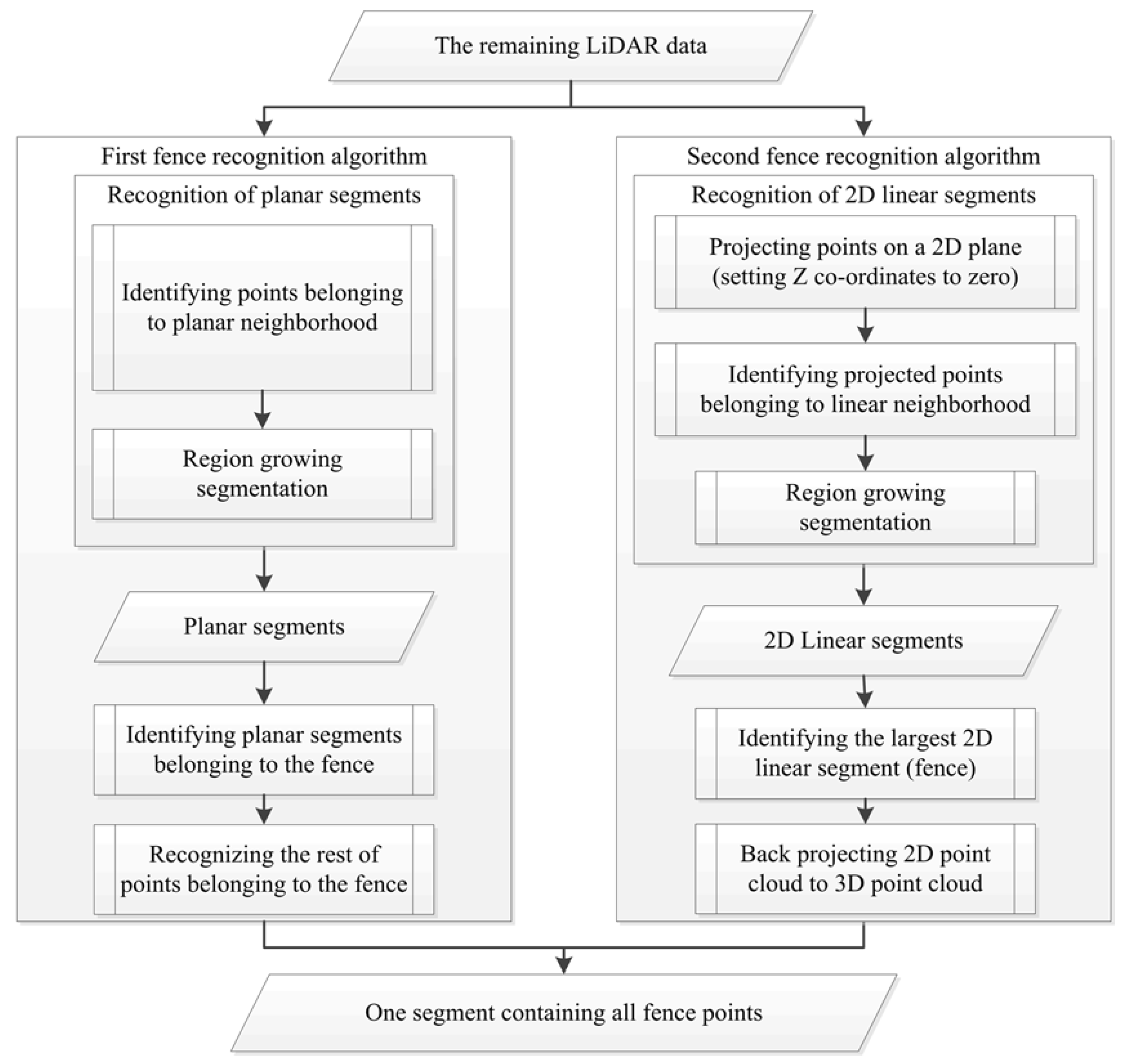
The chain link structure of the fence makes it a penetrable surface. As a result, some planar parts of the fence may be sparsely sampled. Thus, two algorithms were developed to recognize the fence. The first algorithm recognizes the fence in datasets in which fence panels are well-sampled, which is the case for the first and third datasets, described in
Section 5. The second algorithm is able to recognize the fence without taking the fence point sampling into consideration but is computationally more expensive. The second algorithm is used for the second dataset since the fence in this dataset was sparsely sampled. Flowcharts of both fence recognition algorithms are shown in
Figure 4.
4.2.1. First Algorithm for Fence Recognition
First, three-dimensional PCA is employed to detect points belonging to a planar local neighborhood. To detect planar neighborhoods, following conditions need to be met:
where
nλi is a normalized eigenvalue computed as follows:
The neighborhood size used for inspecting the neighborhood structures and the distance threshold used for segmentation in almost all steps of the proposed methodology in this work was 0.15 m. Where a different value is used in the methodology, its rationale is also explained. This threshold (0.15 m) was chosen by considering the size, sparseness and configuration of objects in electrical substation sites. It was found to provide a reasonable balance between incorporating a sufficient number of neighboring points that provide reliable information about local structure and excluding points on adjacent objects.
Figure 4.
Flowchart of two developed algorithms for fence recognition.
Figure 4.
Flowchart of two developed algorithms for fence recognition.
Points within a 3D Euclidean distance of 0.15 m of one another that satisfy the following two conditions are grouped together in a cluster:
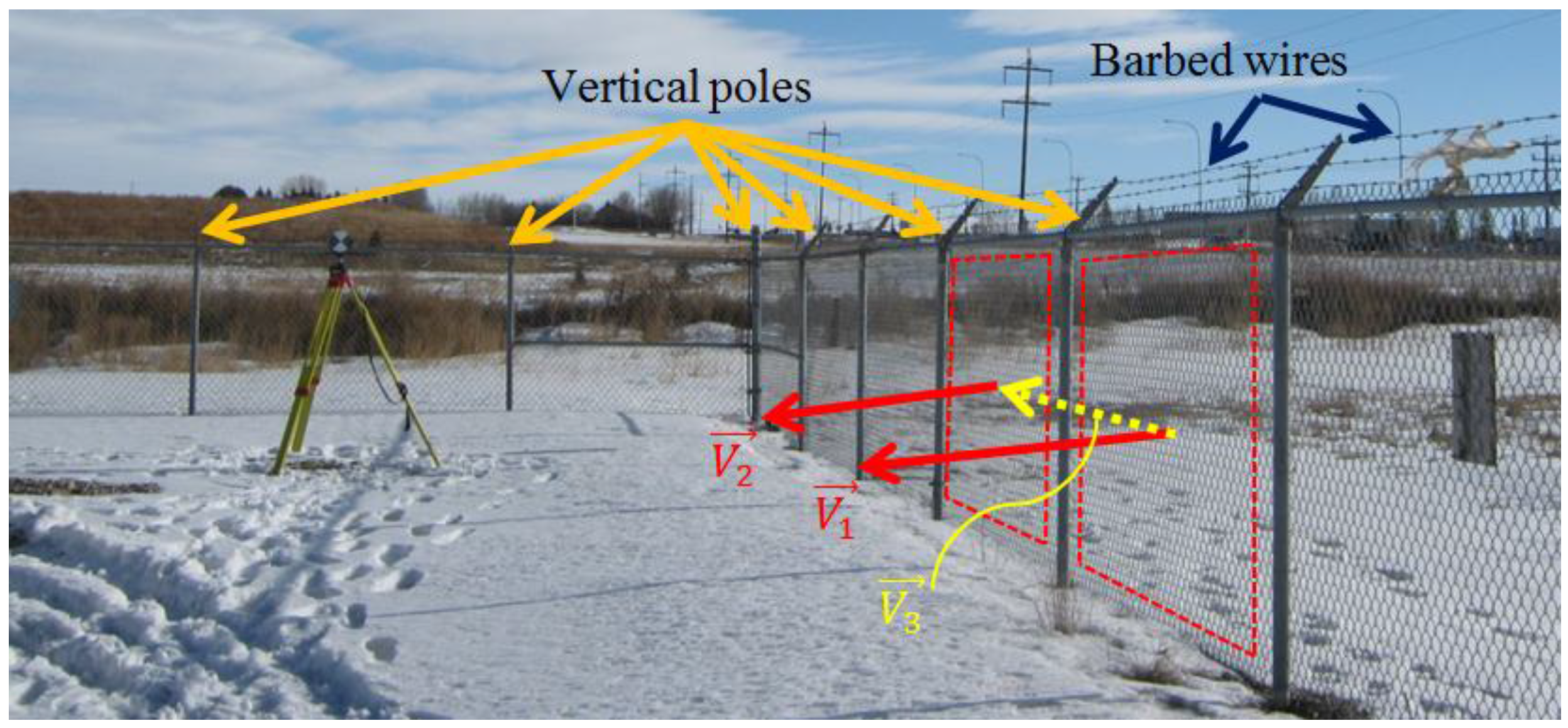
Vertical poles between planar parts of the fence prevent fence points from being clustered into one single segment, as indicated in
Figure 5. Hence, the planar fence segments need to be discriminated from planar segments belonging to other objects. To this end, the following two conditions (see
Figure 5) must be satisfied for at least four adjacent planar segments (since no other object has this many adjacent planar segments): the normal vectors of adjacent planar segments should be parallel (as in Equation (5)) and the vectors connecting the centroids of adjacent planar segments should be perpendicular to the normal vectors (as in Equation (6)).
Figure 5.
Fence recognition by detecting adjacent parallel planar segments, separated by vertical poles. The dashed polygons rectangles represent two planar segments.
Figure 5.
Fence recognition by detecting adjacent parallel planar segments, separated by vertical poles. The dashed polygons rectangles represent two planar segments.
where
and
denote the normal vectors of planar segments and
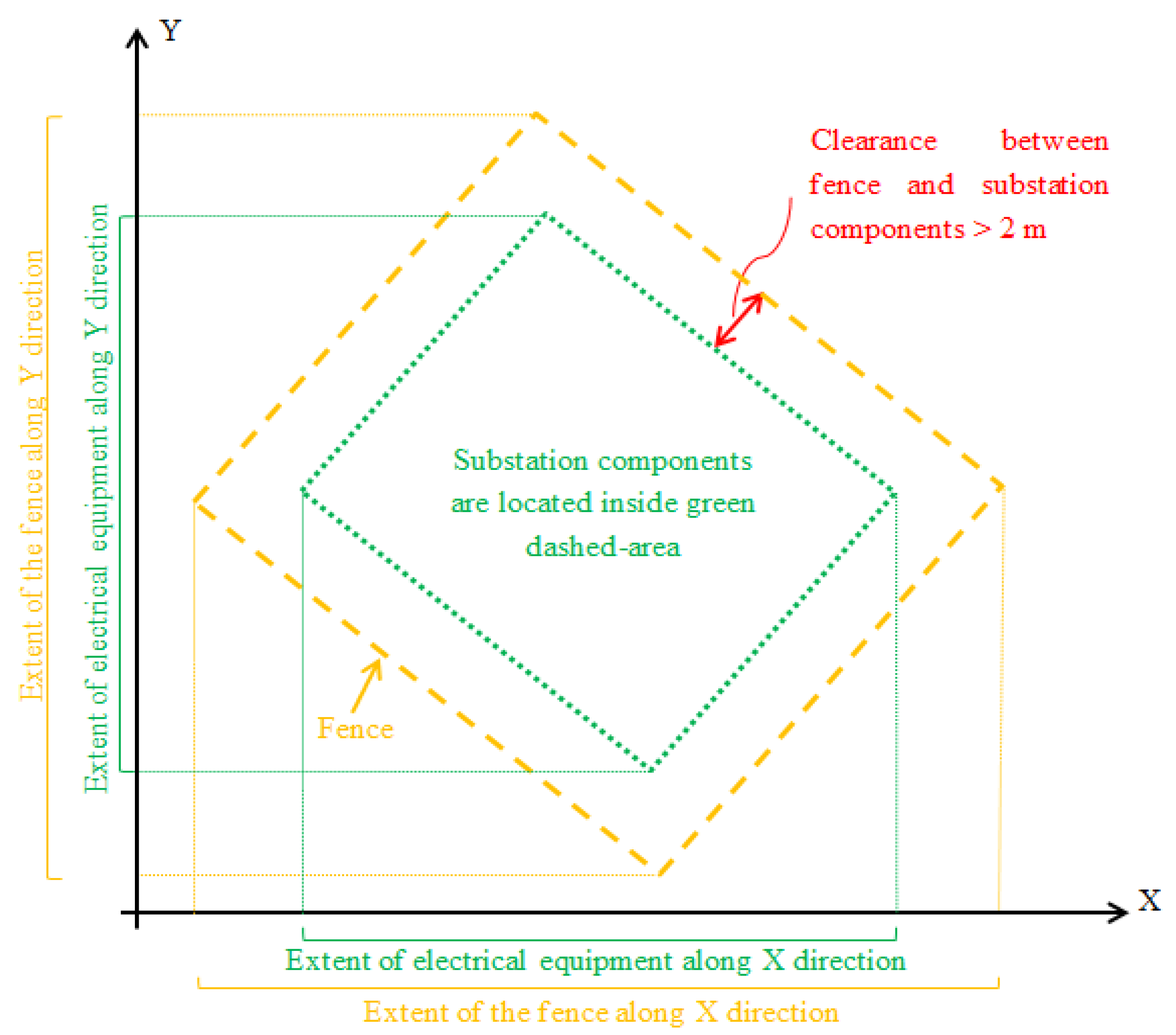
is the vector that connects their centroids. Afterwards, region growing is employed to recognize the remaining parts of the fence (poorly-sampled panels and vertical poles) and also to agglomerate the recognized segments. The region growing algorithm then randomly chooses a seed point from the identified fence points and clusters points within 2-m 3D Euclidean distance. This process is repeated until no more un-segmented points remain within the 2-m threshold. The region growing distance threshold was selected based on prior knowledge of the required safety clearance between the fence and other electrical elements (
Figure 6). The result is that all points belonging to fence are clustered in one segment.
Figure 6.
The clearance between the fence and other components in a substation site (plan view).
Figure 6.
The clearance between the fence and other components in a substation site (plan view).
4.2.2. Second Algorithm for Fence Recognition
This algorithm recognizes the fence based on its planimetric extent. First, all points are projected onto the horizontal plane. Since the fence is vertically distributed, the projected points appear as a linear feature. Other substation objects, such as cables and horizontally oriented bus pipes, also appear as linear objects once projected in this way. However, since the fence encloses the substation, it has the largest planimetric areal extent among all objects on a substation site, as is evident in
Figure 6. Next, 2D eigenvalue analysis is performed to identify points belonging to a linear neighborhood,
i.e.,
Region growing commences by randomly choosing one of points belonging to a linear neighborhood as a seed point. The algorithm then agglomerates all linear-neighborhood points within the 2-m 2D Euclidean distance of the seed point until no linear neighborhood remain. The result is a set of linear segments and the longest linear segment defines the fence.
4.3. Cable Recognition
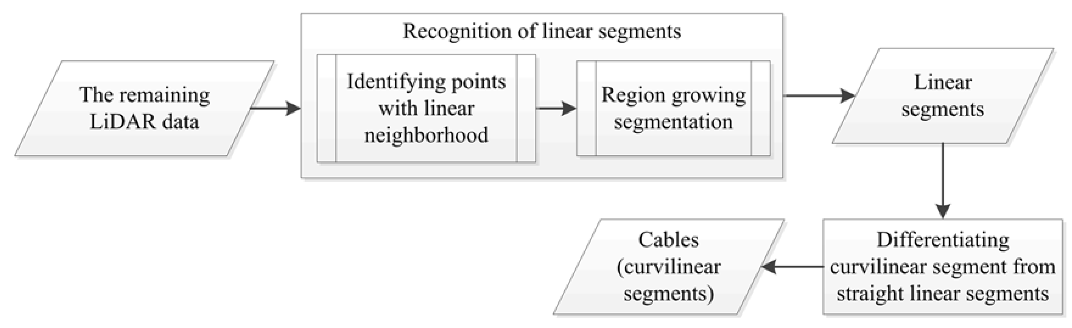
Cables and some incompletely-scanned poles are two types of linear objects that appear in electrical substation LiDAR data. Cables appear as curvilinear objects while partially-scanned poles appear as straight linear objects. Thus, as the flowchart indicates in
Figure 7, linear objects are first identified and then curvilinear objects are differentiated from straight linear objects.
Figure 7.
Flowchart of cable recognition.
Figure 7.
Flowchart of cable recognition.
First, eigenvalue analysis is performed to detect points belonging to linear neighborhoods. The following condition is used to identify points belonging to a linear neighborhood:
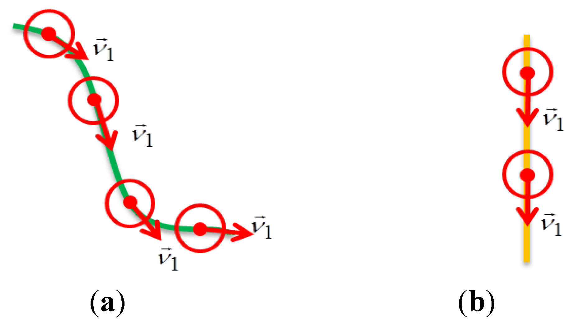
Afterwards, a region-growing algorithm similar to the algorithm used in the second fence recognition algorithm is employed to segment points belonging to a linear neighborhood. The result is a set of linear segments that include cables and non-cable straight linear segments. Cables are distinguished on the basis of their curvature. A cable and a non-cable straight linear segment are shown in
Figure 8 in which red points indicate sample query points, red circles represent their 0.15 m 3D spherical neighborhoods and red arrows point to their principal direction vectors estimated by
(eigenvector corresponding to the largest normalized eigenvalue). As is evident in this figure, the principal direction vectors along the cable vary from point to point (representing the cable’s curvature) but they do not vary along the pole (indicating the pole’s straightness).
Figure 8.
Principal orientation vectors along a cable (a) and along a pole (b). The arrows point to the principal direction within local neighborhoods.
Figure 8.
Principal orientation vectors along a cable (a) and along a pole (b). The arrows point to the principal direction within local neighborhoods.
The standard deviations of three components of
,
i.e., (
vx,
vv,
vz), for all points of each linear segment are used to distinguish between cables and poles. Poles have nominally zero-valued standard deviations in all three dimensions (Equation (9)) since there is no variation in the direction vectors on a pole. Cables have at least one non-zero standard deviation along one of the three cardinal directions, as in Equation (10).
where
,
and
are standard deviation of
three components in the three cardinal directions.
4.4. Recognition of Circuit Breakers and Bushings
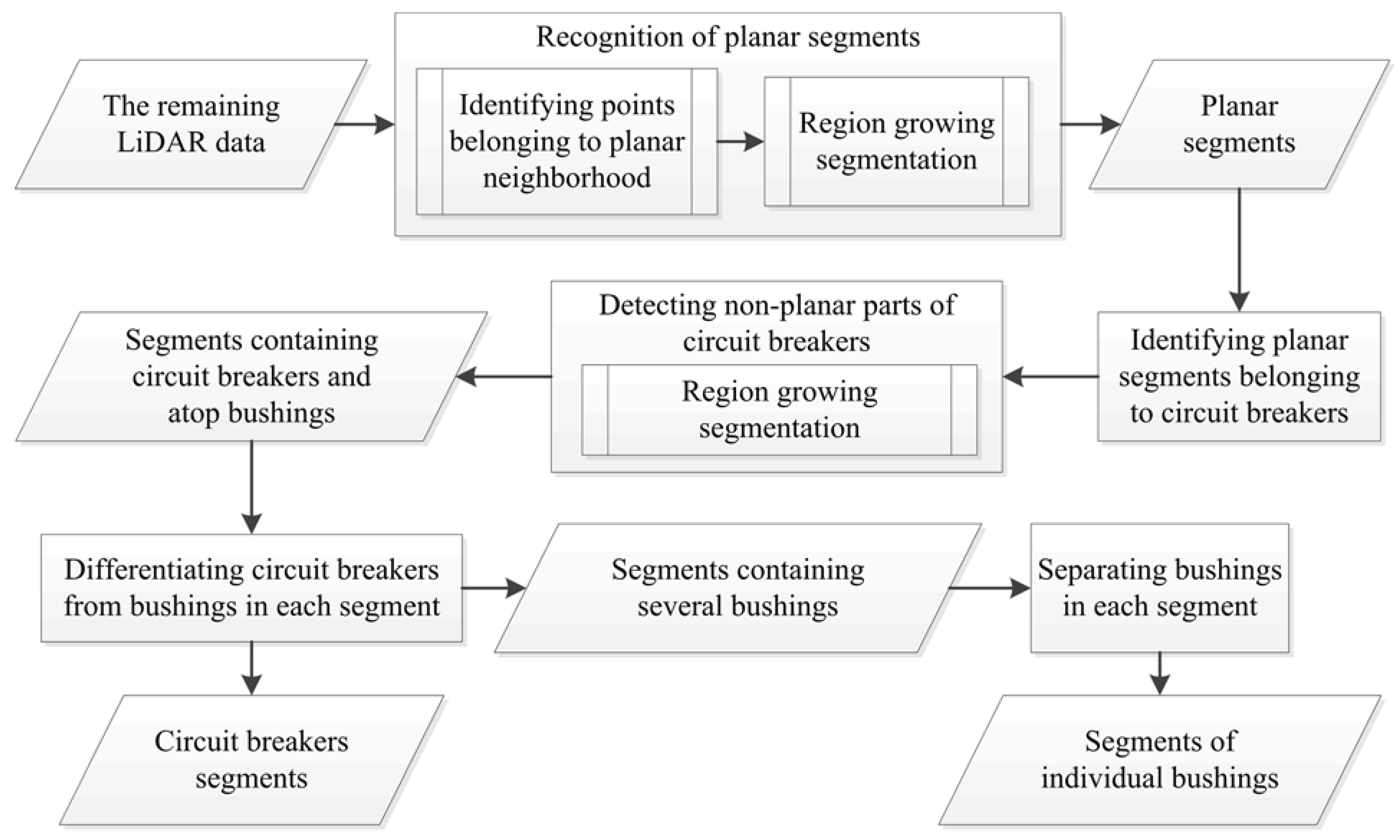
The remaining planar segments identified in the fence recognition step are further analyzed to detect the circuit breakers and the bushings. The flowchart of circuit breaker and bushing recognition is given in
Figure 9.
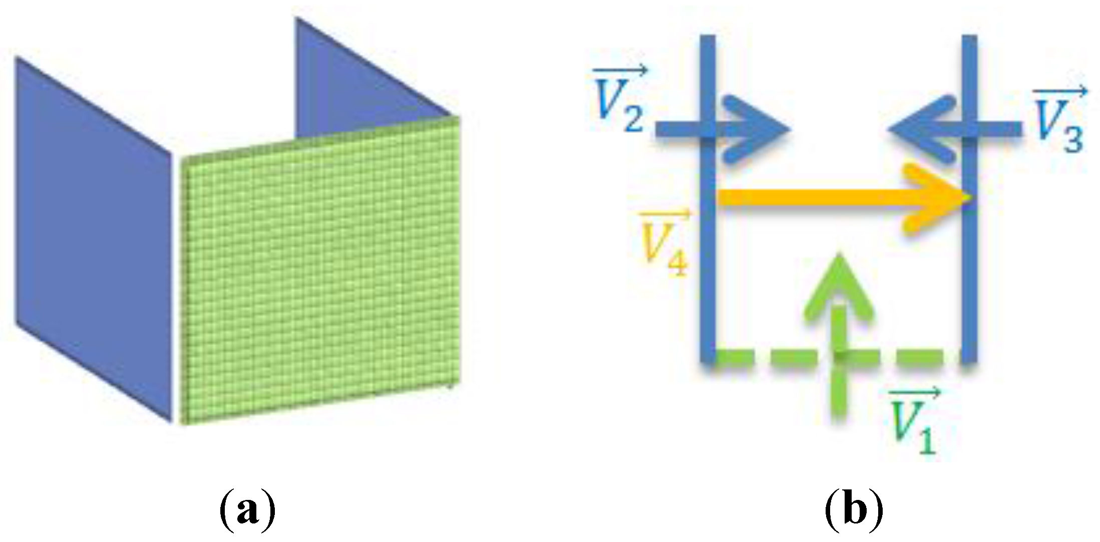
The topological structure common to both types of circuit breakers is one plane bounded by two adjacent perpendicular planes, as shown in
Figure 10. Two following criteria are employed to test if such a structure exists:
If both these criteria are satisfied, then the three planar segments are grouped into one segment and identified as a circuit breaker. Afterwards, region growing is used to recognize the un-recognized parts of the circuit breakers: the non-planar parts; the fourth plane of a regular circuit breaker; and the cylindrical part of an oil circuit breaker. The recognized points on circuit breakers are considered as seed points. Seed points are randomly chosen and points within 0.15 m 3D Euclidean distance are clustered. The growing continues until no more un-segmented point is left in close neighborhood of seed points. The region growing does not include any points belonging to other objects since the only nearby objects are bushings above them, which are topped by cables. Recall that the ground is removed in the first step and cables are recognized in the second step. As a result, all points on each circuit breaker and bushings on top are aggregated in one segment.
Figure 9.
Flowchart of circuit breaker and bushing recognition.
Figure 9.
Flowchart of circuit breaker and bushing recognition.
Figure 10.
The structure common in both two types of circuit breakers consisting of a plane with two adjacent planes in oblique view (a) and plan view (b). The normal vectors of the plane under study and the two adjacent planes are denoted by , and , respectively. The vector connecting the centroids of two adjacent planes is denoted by .
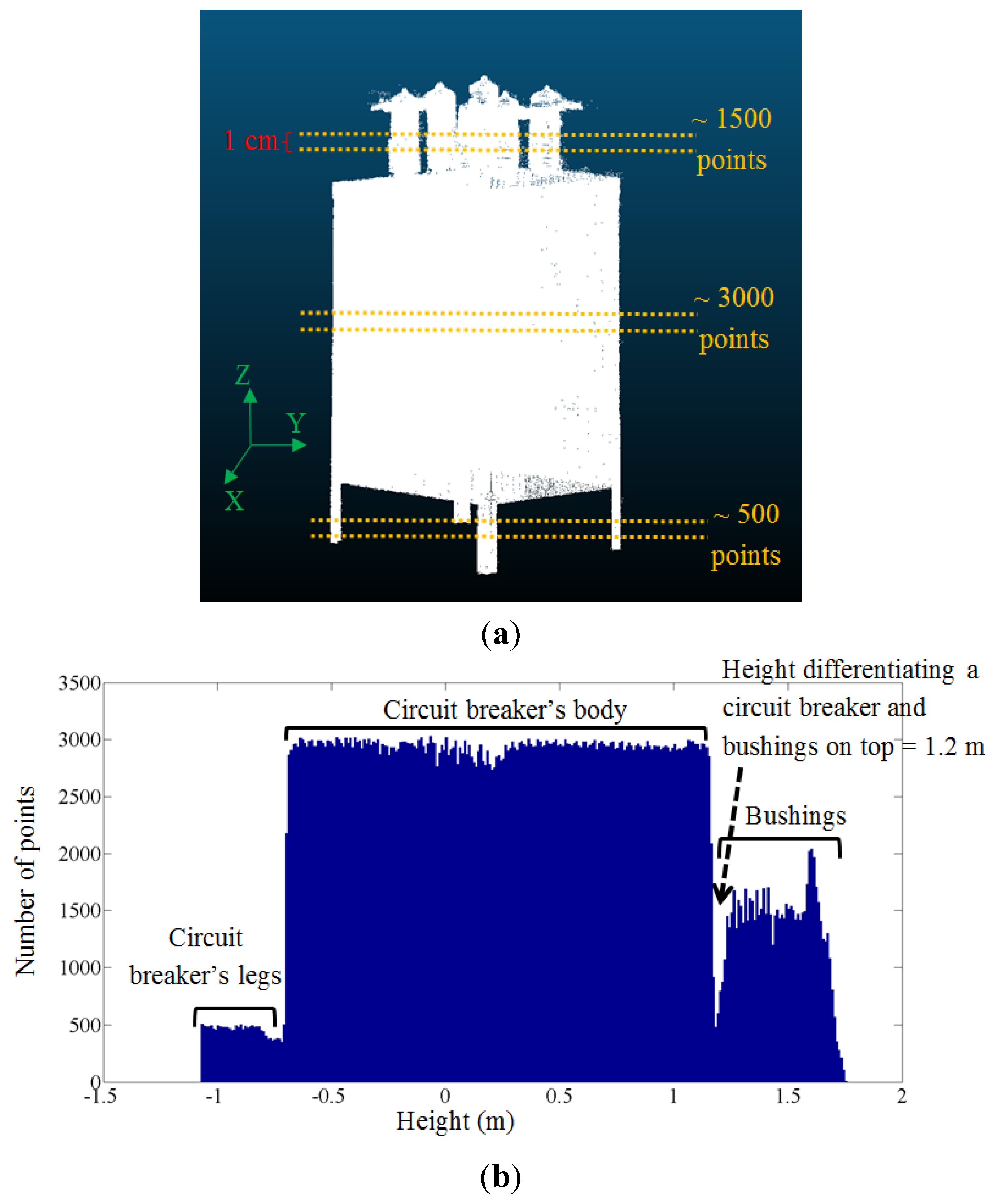
Bushings, which sit atop a circuit breaker, are then separated on the basis of height. A circuit breaker’s body, legs and bushings are identified by inspecting the height histogram. Each segment is divided into 0.1 m wide slices along the vertical direction (horizontal cross section). The bin size needs to be larger than the height accuracy (0.005 m in this case) so that the local point density is correctly reflected in the histogram.
Figure 11a presents an example of a segment containing a circuit breaker and six bushings and
Figure 11b shows the corresponding histogram. A few points on the topmost part of the circuit breakers planar parts may be incorrectly assigned to the bushing segments.
Figure 11.
A segment containing a circuit breaker topped with six bushings is divided to slices in vertical direction (a). Histogram of slices’ points number (b).
Figure 11.
A segment containing a circuit breaker topped with six bushings is divided to slices in vertical direction (a). Histogram of slices’ points number (b).
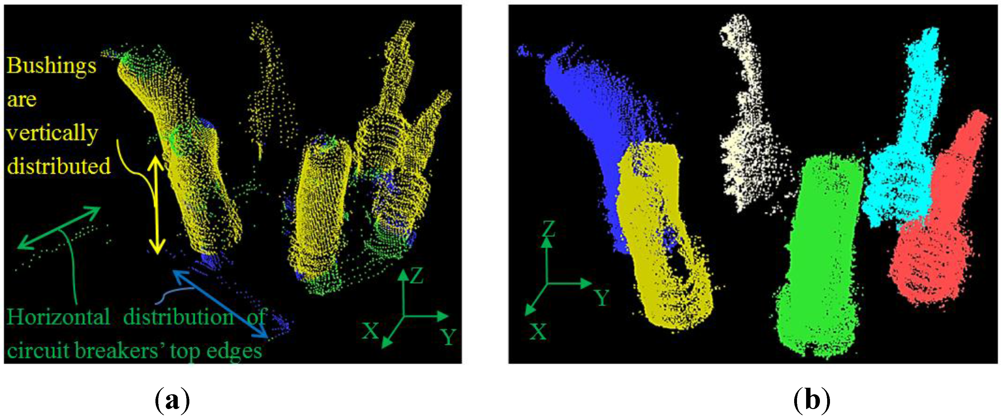
The bushings are separated from one another and from the circuit breaker edges. Bushings are attached to the circuit breaker at the bottom and are separated from each other by a certain clearance (greater than 0.1 m) as required by safety restrictions. Their point clouds are predominantly vertically distributed while points on circuit breakers’ top edges are mainly horizontally distributed. Therefore, the extents of each point’s neighborhood along three cardinal directions are calculated. The largest extent represents the primary distribution direction and the horizontally distributed neighborhoods (belonging to circuit breakers’ top edges) are discarded. Next, points belonging to vertically distributed neighborhoods that are within 0.05 m 3D Euclidean distance of one another are clustered so that each bushing belongs to a separate segment (
Figure 12). The distance threshold (0.05 m) is selected considering the clearance among bushings (greater than 0.1 m).
Figure 12.
Bushings (yellow) are vertically distributed while circuit breakers edges (blue and green) are distributed in horizontal directions (a). Each individually recognized bushing is indicated by a different color (b).
Figure 12.
Bushings (yellow) are vertically distributed while circuit breakers edges (blue and green) are distributed in horizontal directions (a). Each individually recognized bushing is indicated by a different color (b).
4.5. Bus Pipe Recognition
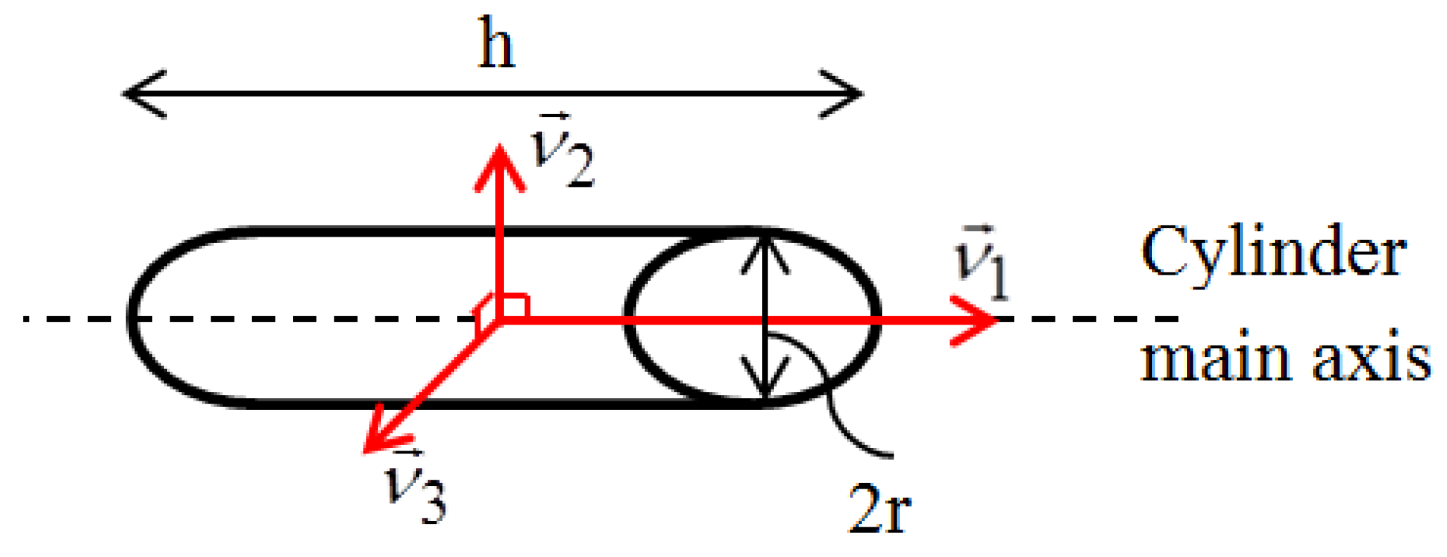
Bus pipes in electrical substations appear as cylindrical-shaped poles whose length is much larger than their radius. Their length easily reaches to several meters while their radius is approximately 0.04 m. First, eigenvalue analysis is employed to detect points belonging to a cylindrical neighborhood. Since bus pipes are mostly distributed along their main axis, the largest normalized eigenvalue (
nλ1) is much larger than other two normalized eigenvalues (
nλ2,
nλ3) and its corresponding eigenvector (
) defines the cylinder axis (
Figure 13). A point is considered to belong to a cylindrical neighborhood if:
Figure 13.
Eigenvectors within cylindrical neighborhood of bus pipes, considering h >> r.
Figure 13.
Eigenvectors within cylindrical neighborhood of bus pipes, considering h >> r.
Region growing segments the points identified as belonging to bus pipes by randomly selecting seed points from the set of points having a cylindrical-shaped neighborhood. The following three criteria are used for the aggregation:
where:
Equation (14) tests if the principal direction vectors () of the seed point and a candidate point are parallel. Equation (15) stipulates that the vector connecting the seed point to a candidate point is parallel to of the seed point. Equation (16) checks whether the height of a candidate point is almost the same as the height of the seed point.
If a candidate point satisfies all three above conditions, it is clustered and this process is pursued until no more un-segmented points belonging to a cylindrical neighborhood is left. As a result, each cylindrical pole belongs to one segment. The thresholds used in Equations (13) and (16) are selected based on standard bus pipes dimensions.
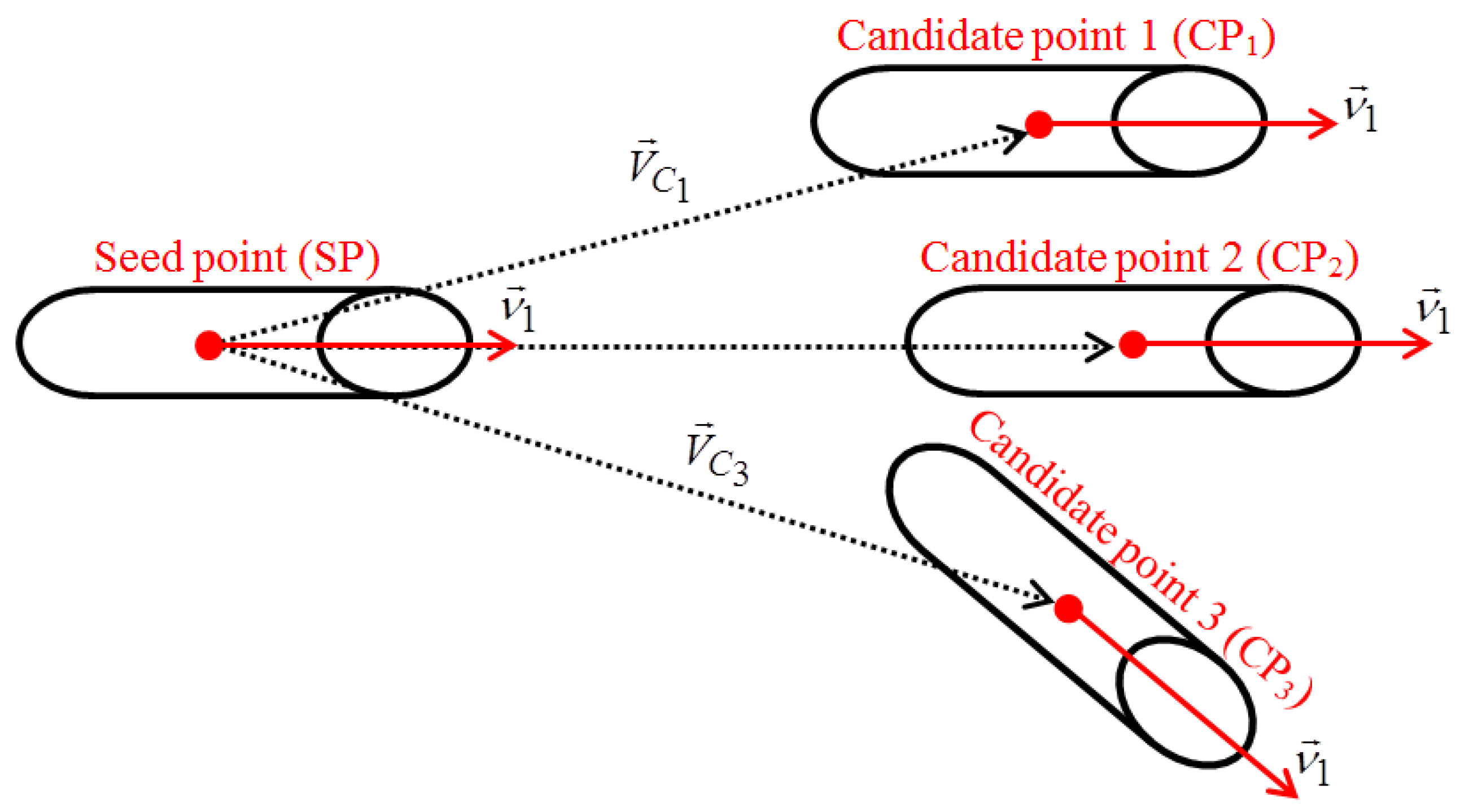
Figure 14 illustrates bus pipe segmentation process in which only CP
2 is merged to the growing segment.
Figure 14.
Bus pipe segmentation process in which all points (incorporating the seed point (SP) and three candidate points (CPi)) are assumed to belong to cylindrical neighborhoods. CP1 is not merged to the growing segment since although it satisfies the first condition (Equation (14)), it does not meet the condition in Equation (15). CP2 is segmented as it meets all criteria. CP3 is also not merged because neither the first condition (Equation (14)) nor the second condition (Equation (15)) is satisfied.
6. Results and Discussion
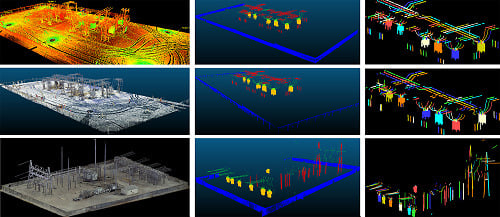
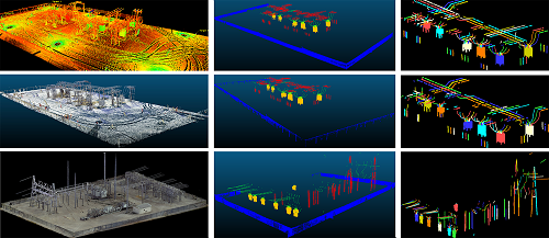
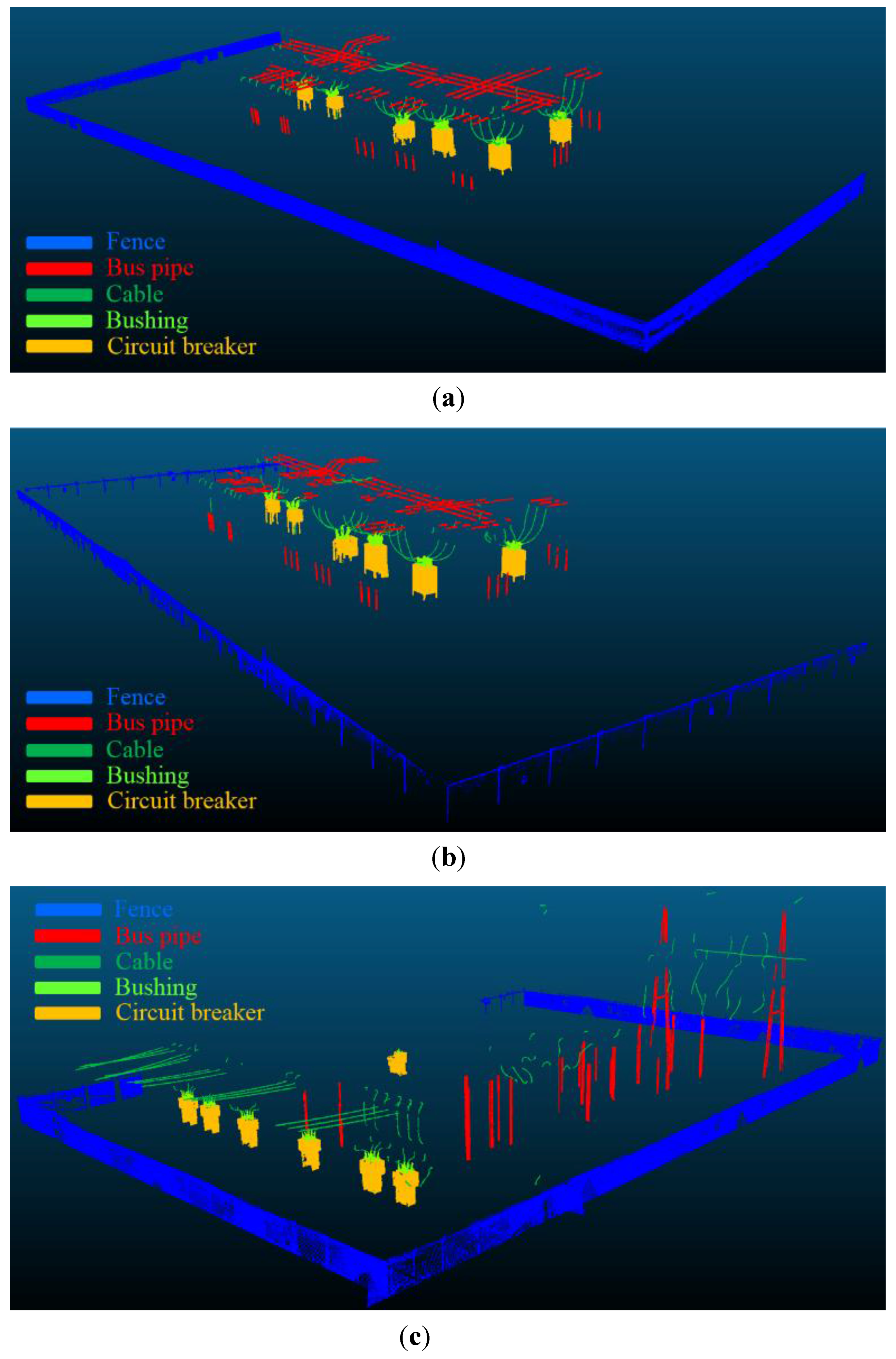
Figure 20 shows the recognized objects in the three datasets. The figure is colorized according to objects’ type.
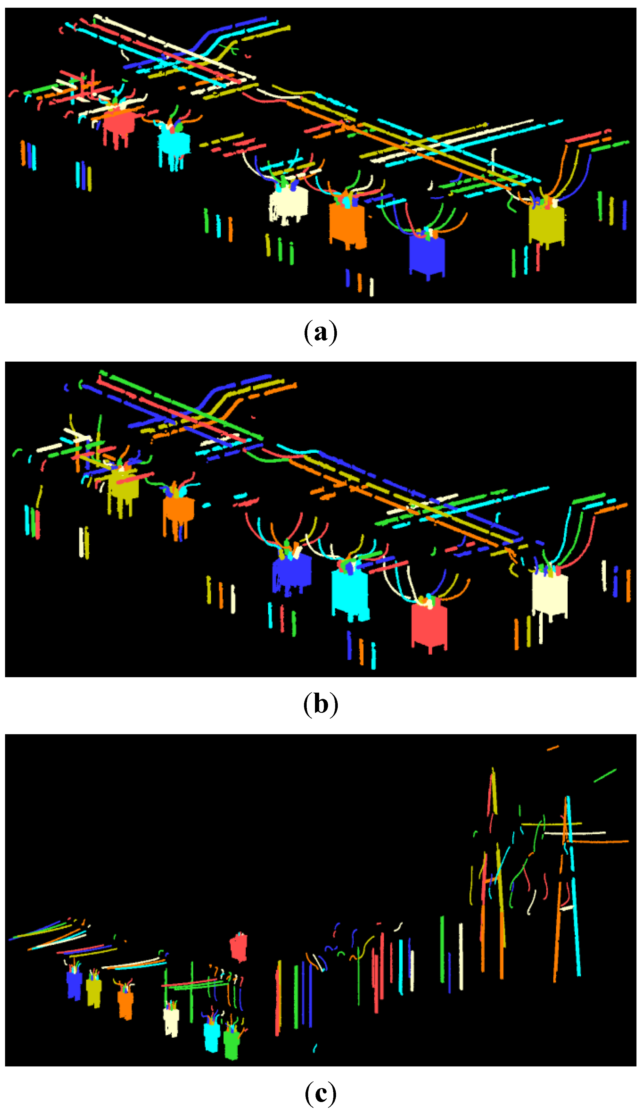
Figure 21 present a finer-level view of the recognized objects in three datasets. Each color in these figures represents a separate segment identified as a circuit breaker, a bushing, a cable or a bus pipe. Moreover, as these figures show, points on the ground in all three datasets have been successfully eliminated.
Figure 20.
Recognized object types in the first dataset (a), second dataset (b) and third dataset (c). Each color represents a different type of object.
Figure 20.
Recognized object types in the first dataset (a), second dataset (b) and third dataset (c). Each color represents a different type of object.
Figure 21.
A finer-level of representation of recognized objects in the first dataset (a), second dataset (b) and third dataset (c). Each color represents a separate object that can be of any type.
Figure 21.
A finer-level of representation of recognized objects in the first dataset (a), second dataset (b) and third dataset (c). Each color represents a separate object that can be of any type.
To assess the results, objects of interest were manually delineated from the original point clouds and were used as ground truth data (presented in
Table 3). The results assessment is presented in
Table 4 in terms of the recognition accuracy and precision at the point cloud level and in
Table 5 in terms of the number of the recognized objects at the object level. Accuracy and precision are calculated as follows.
Where
tp,
tn,
fp and
fn denote the number of true positive, true negative, false positive and false negative occurrences, respectively.
Table 4.
Accuracy and precision of object recognition at point cloud level (in percentage).
Table 4.
Accuracy and precision of object recognition at point cloud level (in percentage).
| Objects | 1st Dataset | 2nd Dataset | 3rd Dataset |
|---|
| Accuracy | Precision | Accuracy | Precision | Accuracy | Precision |
|---|
| Fence | 99.7 | 100 | 98.1 | 100 | 96.7 | 100 |
| Cables | 98.5 | 97.6 | 92.8 | 90.66 | 93.2 | 93.78 |
| Circuit breakers | 100 | 100 | 100 | 100 | 100 | 100 |
| Bushings | 100 | 100 | 100 | 100 | 100 | 100 |
| Bus pipes | 98.2 | 100 | 92.8 | 100 | 97.1 | 100 |
| Mean | 99.28 | 99.52 | 96.74 | 98.13 | 97.4 | 98.76 |
Table 5.
Recognition results at object level.
Table 5.
Recognition results at object level.
| Objects | 1st Dataset | 2nd Dataset | 3rd Dataset |
|---|
| Recognized Objects | False Positives | Recognized Objects | False Positives | Recognized Objects | False Positives |
|---|
| Fence | 1 (1) | 0 | 1 (1) | 0 | 1 (1) | 0 |
| Cables | 68 (69) | 1 | 64 (69) | 3 | 109 (117) | 2 |
| Circuit breakers | 6 (6) | 0 | 6 (6) | 0 | 7 (7) | 0 |
| Bushings | 36 (36) | 0 | 36 (36) | 0 | 39 (39) | 0 |
| Bus pipes | 67 (69) | 0 | 64 (69) | 0 | 27 (27) | 0 |
| All objects | 178 (181) | 1 | 171 (181) | 3 | 183 (191) | 2 |
The high mean recognition accuracy of the fence (98.2%) suggests that the majority of points belonging to fence are recognized. The highest fence recognition accuracy was achieved for the first dataset, which was anticipated due to the finer point sampling of the fence in this dataset. Although average point sampling on the fence was higher for the third dataset than for the second, the associated fence recognition accuracy was slightly lower (less than 2%). This is due to non-uniform point sampling of the fence in the third dataset: some fence panels were very well-sampled while others were very poorly-sampled.
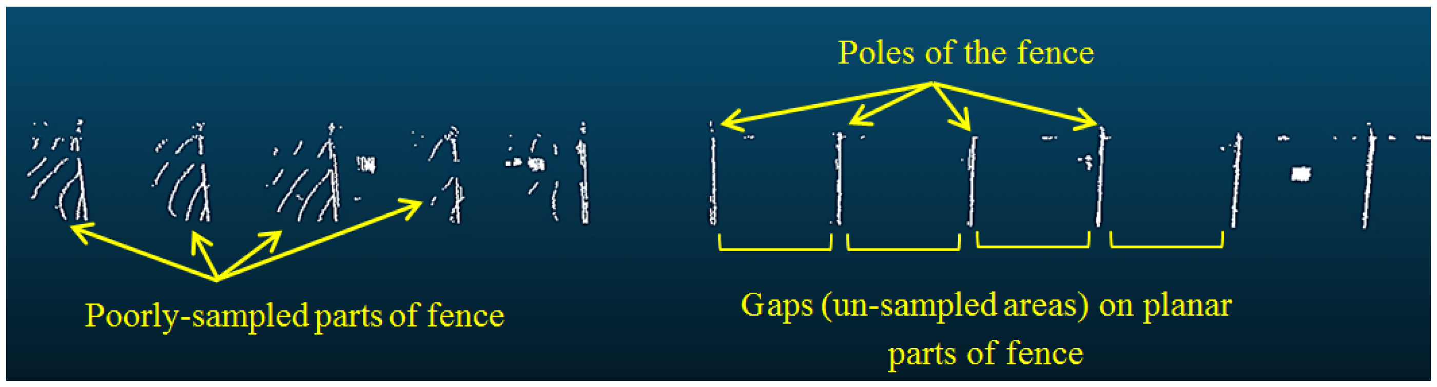
Figure 20c shows an instance of such a poorly-sampled area with large gaps and, as a result, many fence panels were not recognized. Moreover,
Figure 22 depicts some poorly-sampled fence panels suggesting a linear structure while its true structure is planar.
Figure 22 also demonstrates fence recognition failure in a part of data with gaps larger than the 2-m region growing distance threshold. The high recognition accuracy of the sampled portions (especially in the first and second datasets) demonstrates that if the fences were well-sampled, they can be successfully recognized. Furthermore, there are no false positives in the results of fence recognition of all three datasets implying 100% recognition precision. This demonstrates the suitability of using fence’s unique shape (
i.e., multiple adjacent planar surfaces) for its recognition.
Figure 22.
Poorly-sampled parts and gaps (un-sampled parts) of the fence in the third dataset.
Figure 22.
Poorly-sampled parts and gaps (un-sampled parts) of the fence in the third dataset.
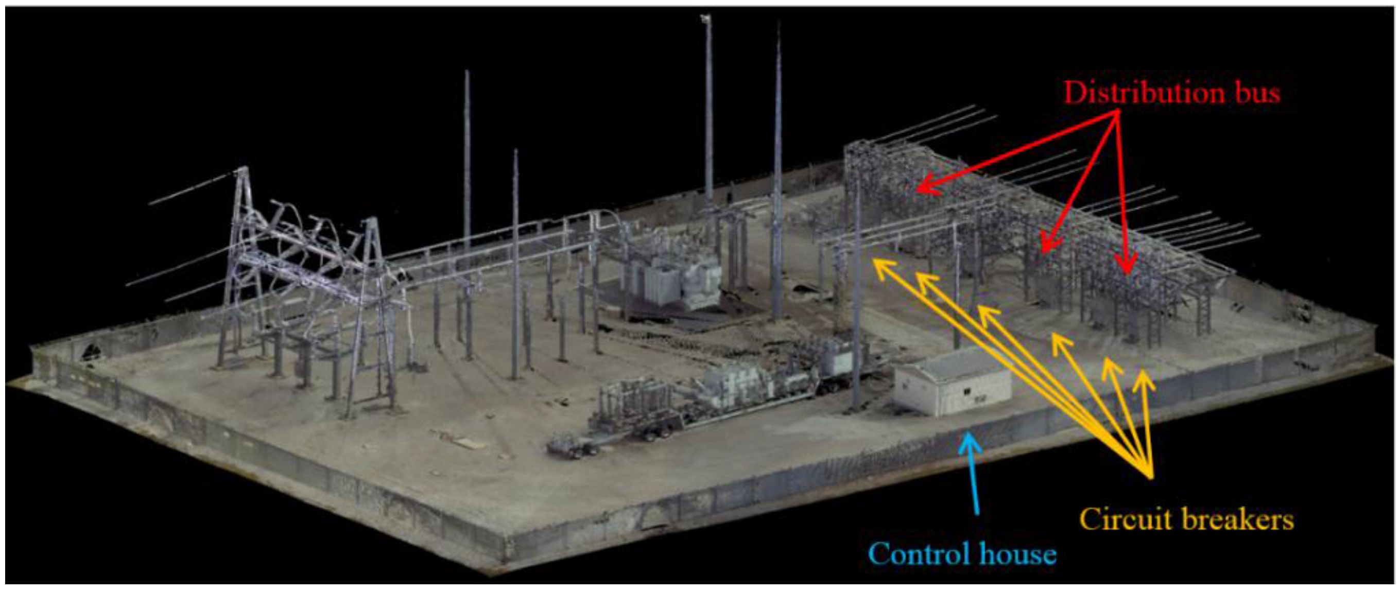
The cable recognition was also very successful as 98.5% of cables in the first dataset were recognized and there was only one false positive. The cables of the second and third datasets were recognized with greater than 92% accuracy. However, there were three false positives in the second dataset and two false positives in the third. The false positives were caused by under-sampled poles that appear as curvilinear objects in the point clouds and were incorrectly recognized as cables. The highest cable recognition accuracy and precision was achieved for the first dataset, which is expected since the associated cable point sampling was the highest among three datasets. Although cable recognition accuracy of the third dataset is quite high (greater than 93%), it is the lowest among three datasets since the majority of cables are situated among the distribution bus components. The distribution bus (as is evident in
Figure 19) has a very dense structure and, as a result, many cables were highly occluded.
The recognition results of the circuit breaker and bushings indicate that all were recognized in all three datasets. There are also no false positives in the results of three datasets, so the recognition precision was 100%. The isolated position of the circuit breakers and bushings has a great impact on their perfect recognition results since they were well-sampled by the laser scanner and occlusions by other objects were quite minimal. This is evident in
Table 3 that indicates circuit breakers have the highest point sampling among all key components in each dataset. Furthermore, exploiting the bushings’ distinctive topology (
i.e., locating between circuit breakers and cables) rather than using their shape for their recognition lead to perfect results, even though they have the most complicated physical shape among all key components of electrical substations.
As indicated in
Table 5, 67 and 64 out of 69 bus pipes in the first and second datasets were recognized. Again, the highest bus pipe recognition accuracy (98.2%) at the point cloud level was realized for the first dataset due to the highest sampling. In the third dataset, all 27 bus pipes were recognized (100% accuracy at the object level) and 97.1% accuracy at the point cloud level was obtained. Although the bus pipe point-sampling of the second and third datasets was almost the same, results are more successful in the third dataset. This stems from denser configuration of bus pipes in the second dataset, which is evident in
Figure 21b,c. Furthermore, there were no false positives in the bus pipe recognition results for all three datasets.
As the results suggest, under-sampling, caused by sparse point coverage and/or occlusions, is the primary cause of the recognition failure and false positives. When a large portion of an object is under-sampled, its form and structure cannot be accurately recognized according to the described rules. However, it is crucial to note that the determining factor for the recognition success is the point sampling of the objects of interest and that considering only the total volume of the datasets in evaluating the results can be misleading. This is evident in the results of the third dataset that has the largest volume among all three datasets while the point sampling of its key components is the lowest. Occlusions and sparse sampling can be ameliorated by acquiring more scans from various locations. This action, however, requires additional time for fieldwork and results in a point cloud with larger volume, which increases computational time and cost and decreases data processing efficiency. Therefore, a balance is required between the number of scan stations and size of the dataset to achieve acceptable recognition results with a reasonable processing time and cost. This balance can be achieved by considering the number, size and configuration of components at an electrical substation site. Furthermore, the local neighborhoods are characterized using PCA, which can be sensitive to noise. As explained in
Section 4, the noise level in the datasets used in this work was quite minimal. However, PCA might not produce reliable information regarding the local neighborhood structure for a dataset with a higher noise level. In such a case, employing RANSAC is recommended.


