Article

Using UAV-Based Photogrammetry and Hyperspectral Imaging for Mapping Bark Beetle Damage at Tree-Level

1
Department of Remote Sensing and Photogrammetry, Finnish Geospatial Research Institute, Geodeetinrinne 2, 02430 Masala, Finland
2
Department of Forest Sciences, University of Helsinki, P.O. Box 27, FI-00014 Helsinki, Finland
*
Author to whom correspondence should be addressed.
Remote Sens. 2015, 7(11), 15467-15493; https://doi.org/10.3390/rs71115467
Submission received: 24 September 2015 / Revised: 6 November 2015 / Accepted: 12 November 2015 / Published: 18 November 2015

Abstract

:
Low-cost, miniaturized hyperspectral imaging technology is becoming available for small unmanned aerial vehicle (UAV) platforms. This technology can be efficient in carrying out small-area inspections of anomalous reflectance characteristics of trees at a very high level of detail. Increased frequency and intensity of insect induced forest disturbance has established a new demand for effective methods suitable in mapping and monitoring tasks. In this investigation, a novel miniaturized hyperspectral frame imaging sensor operating in the wavelength range of 500–900 nm was used to identify mature Norway spruce (Picea abies L. Karst.) trees suffering from infestation, representing a different outbreak phase, by the European spruce bark beetle (Ips typographus L.). We developed a new processing method for analyzing spectral characteristic for high spatial resolution photogrammetric and hyperspectral images in forested environments, as well as for identifying individual anomalous trees. The dense point clouds, measured using image matching, enabled detection of single trees with an accuracy of 74.7%. We classified the trees into classes of healthy, infested and dead, and the results were promising. The best results for the overall accuracy were 76% (Cohen’s kappa 0.60), when using three color classes (healthy, infested, dead). For two color classes (healthy, dead), the best overall accuracy was 90% (kappa 0.80). The survey methodology based on high-resolution hyperspectral imaging will be of a high practical value for forest health management, indicating a status of bark beetle outbreak in time.

Graphical Abstract

1. Introduction

Forest ecosystems are annually faced with incremental disturbances by native and non-indigenous insect pests in the boreal zone [1]. According to the projections of climatic change impacts, distribution of forest pest insects, as well as insect-induced damage will gradually shift towards northern latitudes. This climate-driven phenomenon has already been evident with pine sawflies [2,3], moths [4,5] and bark beetles [6,7]. Rapidly increasing forest disturbances give rise to a threat for forest health and substantial economic losses [8]. Therefore, accurate and cost-efficient detection of stand and tree conditions for timely forest management are needed.
Spatially and temporally significant outbreaks of bark beetles, particularly associated with the Norway spruce (Picea abies L. Karst.), have been evident in the course of time, in mid and eastern parts of Europe, as well as in southern Norway and Sweden [9,10,11]. Since the year 2010, with a high accumulated temperature, the European spruce bark beetle (Ips typographus L. (I. typographus)) (Curculionidae, Scolytinae) has also triggered high tree mortality in south and mid parts of Finland, due to two annual generations of the pest [12]. Mortality of standing trees at a stand level may reach up to 60% on the second or third post-storm year, if a number of wind-felled trees provide plenty of breeding material for beetles [13]. Few years after initial outbreak, tree mortality can be implicit, and may ascend to 100% of trees [14]. A warm and dry climatic pattern with several gales has constituted optimal conditions for I. typographus to reproduce in wind-felled trees [15]. The population growth rate is high in freshly dead wood and weakened trees, reconstructing a focal point of an outbreak. An invasion front of beetles can attack and kill vigorous trees under a high population density [16]. An invasion by I. typographus causes visible crown symptoms, i.e., discoloration and defoliation, before succumbing from the infestation. The crown color transforms due to larval feeding in xylem and phloem tissues, prohibiting water flux from roots to the crown. The initial attack is not visible to the human eye (green attack) [17]. With thousands of attacking beetles per one Norway spruce tree, needles first turn yellow (yellow attack), then to reddish brown (red attack), and finally grey (tree mortality) [18]. According to our experience, this gradual weakening goes on for a few weeks and is highly dependent on bark beetle density and tree resistance. Early detection of the symptoms gives ground for a development of combat measures, based on damage mapping and risk assessment.
Damage monitoring and risk assessment of bark beetles have traditionally been based on laborious and time-consuming field sampling and observations in forest stands, focusing on symptoms on the trunk and foliage [14,19]. However, anomalies in crown health are more visible from a bird’s eye view. Remote sensing, such as aerial images, multi-temporal satellite images and synthetic aperture radar (SAR) datasets, Landsat Thematic Mapper (TM), Moderate Resolution Imaging Spectroradiometer (MODIS), TerraSAR-X and light detection and ranging (LiDAR), have been applied in forest health surveys and detection of disturbances by pest insects [17,20,21,22,23,24]. Mid- and low-resolution remote sensing data have proven to be practical for insect outbreak surveys over wide landscapes. However, typically, insect pest outbreaks in Fennoscandia represent a patchy and uneven pattern, and the forested landscapes are fragmented by mosaics of small stands, suffering from a varying intensity of an infestation [25]. In addition, the rate of private forest ownership is high in Fennoscandia, which introduces a need for tailored, cost-efficient, small-scale operations in private-owned forests, as well as in urban city forests.
The detection of health changes in Norway spruce forests, with hyperspectral remote sensing, has been studied using airborne instruments [26,27,28]. Campbell et al. [26] studied the health of Norway spruce forests in the Czech Republic with an airborne pushbroom imaging radiometer, Advanced Solid-state Array Spectroradiometer (ASAS), with a spectral range of 410–1032 nm. In their study, the spectrum of 673–724 nm provided the highest potential in identifying forests with an initial status of damage. Hyperspectral aerial imagery with a Hyperspectral Mapper (HyMAP) instrument has been used in the detection of a bark beetle infestation in Germany [14,27]. In [14], classification of the different attack stages was typically based on wavebands within the spectral range of 450–890 nm, that are related to prominent chlorophyll absorption features. They observed that hyperspectral data with a ground resolution of 4 m provided more relevant information in estimation of the vitality of spruces compared to data with a ground resolution of 7 m. In their study, spruces with green foliage but reduced vitality were classified with an accuracy of 64%. According to [14], the result was considered insufficient in forestry practices. Fassnacht et al. [27] used the same data as [14] and detected infested trees with an error of commission of 65%. They found that accurate differentiation of the three vitality classes was not possible with the used methodology. However, the required accuracy of classification is dependent on demands of an end-user and on the nature of a disturbance case.
Studies utilizing unmanned airborne vehicles (UAV) in forest health monitoring are scarce. One of the first published efforts to detect insect damage in a forest ecosystem applying UAV was a study in Germany [28]. They used multispectral imagery and object-based image analysis to detect an infestation in oak stands (Quercus sp.) by the oak splendor beetle (Agrilus biguttatus Fab.). In agriculture, tree health monitoring with hyper or multispectral UAV data and image analysis has been studied, for example, in olive orchards [29] and citrus trees [30]. A UAV-based, tree-wise monitoring system in detection of early symptoms of insect-induced disturbance in evergreens would be of high value in forest health management operations that aim to prevent further development of forest pest populations and tree mortality in damage spots.
Photogrammetrically produced UAV Digital Surface Models (DSM) and Canopy Height Models (CHM) that allow for detecting individual tree crowns in forests have been computed in [31] and [32]. The density and accuracy of 3D point clouds produced by methods in [32] across forested landscapes were deemed sufficient for general forestry applications. In forest inventory using remote sensing, structural forest attributes are typically extracted from the CHM by means of regression models predicting forest variables such as mean height, dominant height, stem number, basal area, and stem volume, with descriptive statistic of the canopy height model on a particular area. The forest owners need information for monitoring and planning timely thinning and harvesting. In environmental monitoring, forest biomass and carbon stock estimation benefit from accurate and valid (up to date) CHMs. Photo-CHM and LiDAR-CHM window-based metrics were found to be well correlated in [31], and individual tree heights were comparable with LiDAR metrics. Regression models at stand or plot level using point clouds from UAV imagery provided accurate and timely forest inventory information on a local scale. In [31], individual tree height could be estimated from UAV photo CHM with RMSE of 1.04 m and R2 of 0.91. In [32], CHMs from imagery and LiDAR DTM were strong predictors of field-measured tree heights with R2 of 0.63 to 0.84. In [33], plot level linear models for Lorey’s mean height and dominant height were computed; the respective cross validated RMSE values were 1.4 m and 0.7 m.
The aim of this study was to investigate the potential of novel UAV-based 3D hyperspectral remote sensing technique in identifying symptoms by bark beetle attack of different intensity in mature Norway spruce forest. We used a remote sensing system consisting of a Fabry–Pérot Interferometer (FPI) based miniaturized hyperspectral camera and a consumer color camera with red, green and blue bands (RGB). A novel feature of the FPI technology is that by collecting frame-format hyperspectral images, it allows stereoscopic and hyperspectral analysis of the object, as well as generation of dense point clouds and DSMs. This was not possible with the conventional hyperspectral instruments based on whiskbroom or pushbroom scanning. Our objectives were to implement the entire processing line for capturing 3D information and spectral data of individual trees from the novel UAV-based imaging system, as well as to investigate the potential of this technology in identifying symptoms by bark beetle attack.

2. Materials and Methods

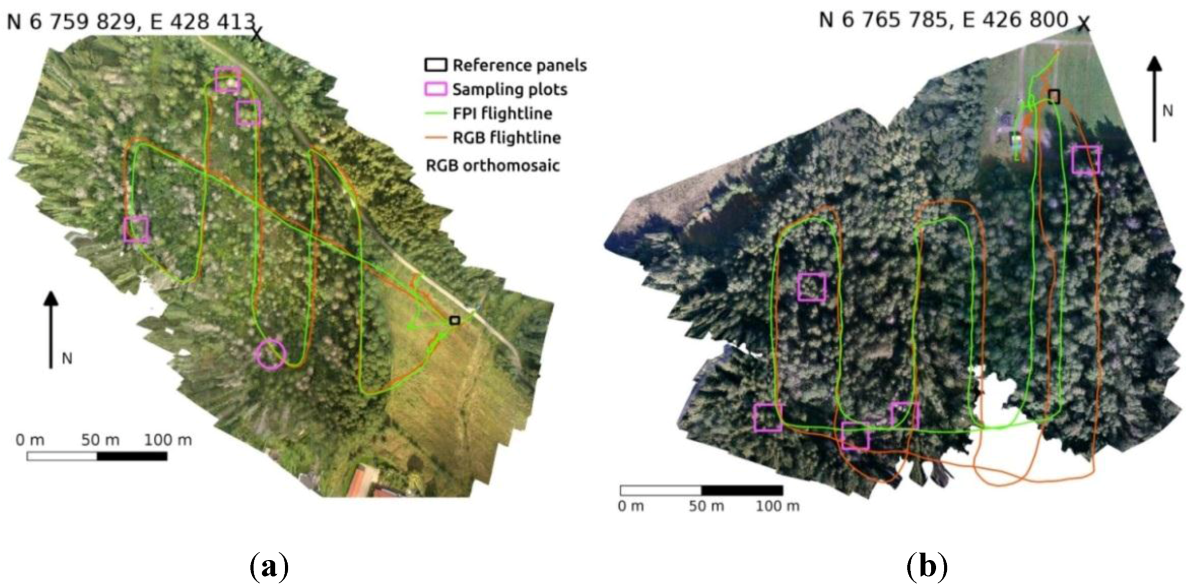
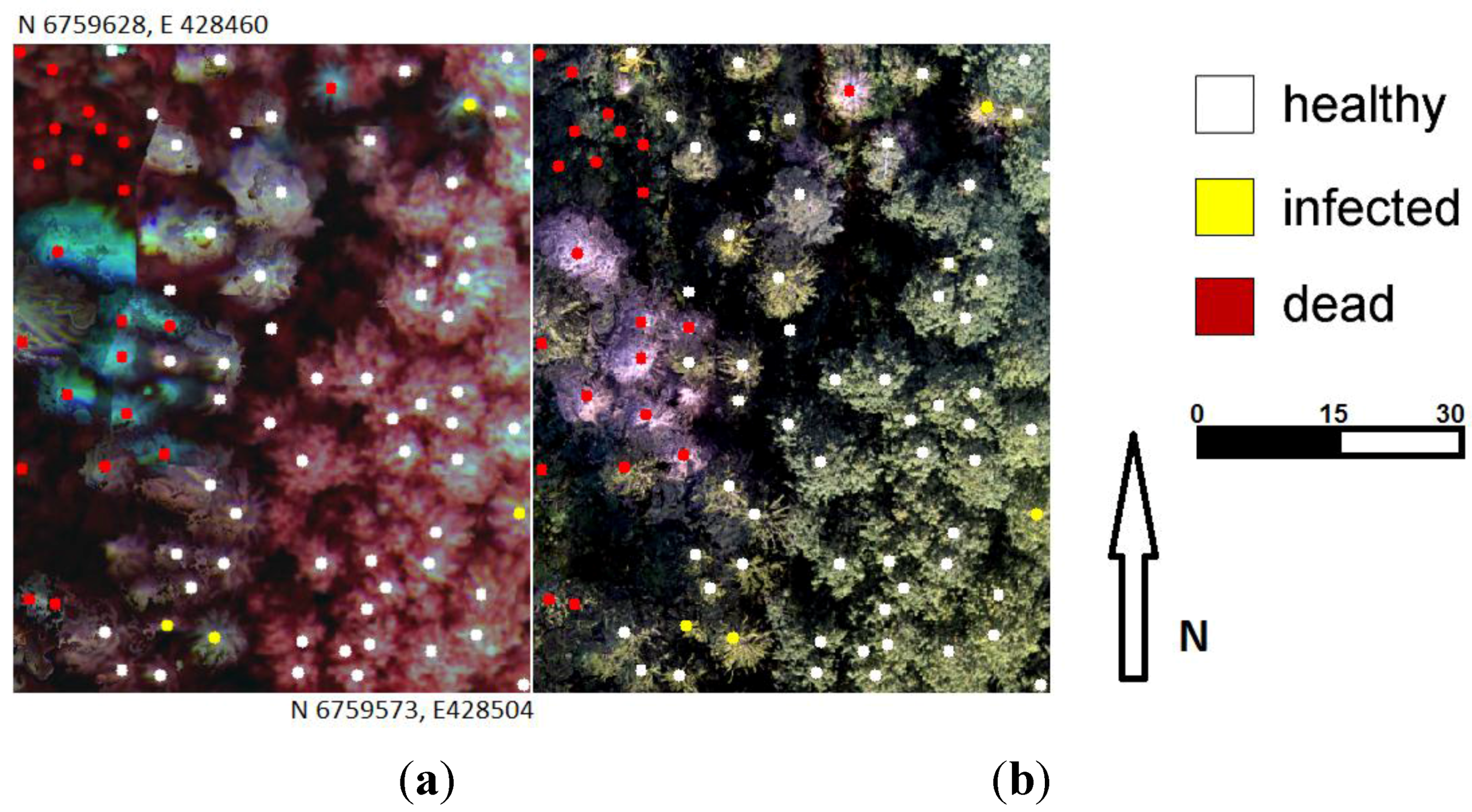
2.1. Test Area and Ground Truth

The study area is located in southern Finland, in the city of Lahti (60°59′N, 25°39′E). These urban forests are mostly dominated by mature Norway spruce, growing on fertile soils (Oxalis-Maianthemum type and Myrtillus type) [34]. The total coverage of the urban forest in the city of Lahti is about 5000 ha. I. typographus has caused damage and tree mortality within the area since 2010. We established nine circular sampling plots (radius = 10 m) in two test areas of Mukkula and Kerinkallio, where the dominated Norway spruce trees covered approximately 90%–95% of the two upper canopy layers. One of the plots was already established in 2012, seven in 2013 and one in 2014. The center of each plot was located with a Trimble Geo XT GPS-device (Trimble Navigation Ltd., Sunnyvale, CA, USA). Individual trees were located by measuring the distance and azimuth to each tree from the plot center.
Tree-wise measurements (Table 1) were conducted annually in August, because the symptoms are visible to the human eye late in the growing season. Diameter-at-breast-height (cm) was measured for each tree. Tree height of median trees of the plots and every seventh tree were measured. The field observations included classification of visual tree-wise symptoms, such as crown discoloration and defoliation, indicating invasion status of the I. typographus. In the fieldwork, the crown color was classified as green (healthy, class 1), yellowish (yellow attack, class 2), reddish (red attack, class 3) and grey (dead tree, class 4). Healthy trees and trees with a potential early infestation stage (green attack) were not separated with the present study. We did not measure non-UAV based reflectance spectra for different crown color classes. We eliminated small reference trees that were likely to be in the shadows of the larger trees; these included trees with a DBH under 25 cm and trees with very low reflectance values (average reflectance in the processed images under 0.03). Finally, a total of 78 mature Norway spruces from the two upper canopy cover layers were available for the analysis (Table 1 and Table 2). Due to lack of the reddish crowns, this class was excluded from the analysis.
Table 1. Statistics of the sampled trees in the different crown color classes. Healthy (green), class 1; infested (yellowish), class 2; and dead (grey), class 4. D is diameter-at-breast-height (cm) and H is tree height (m); mean, min, max and sd are the average, minimum, maximum and standard deviation of measurements, respectively.
2013nDmeanDminDmaxDsdHmeanHminHmaxHsd
Healthy3637.426.260.28.429.723.935.34.6
Infested1543.429.762.010.430.825.934.84.3
Dead2739.626.852.77.630.229.332.01.3
Table 2. Numbers of trees in the different crown color classes in two test areas.
AreaHealthyInfestedDeadTotal
Mukkula264939
Kerinkallio10111839

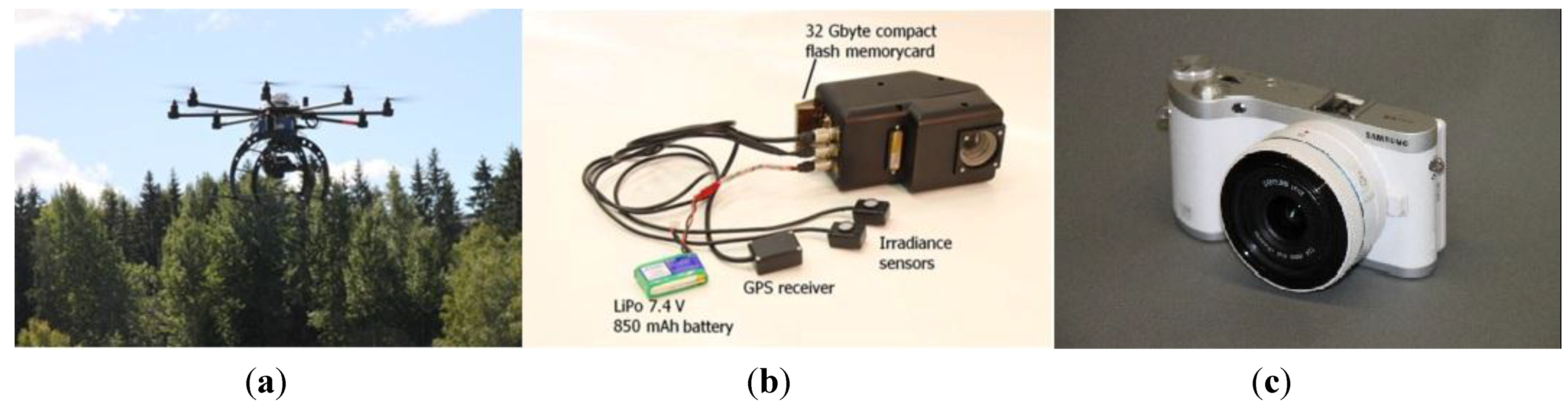
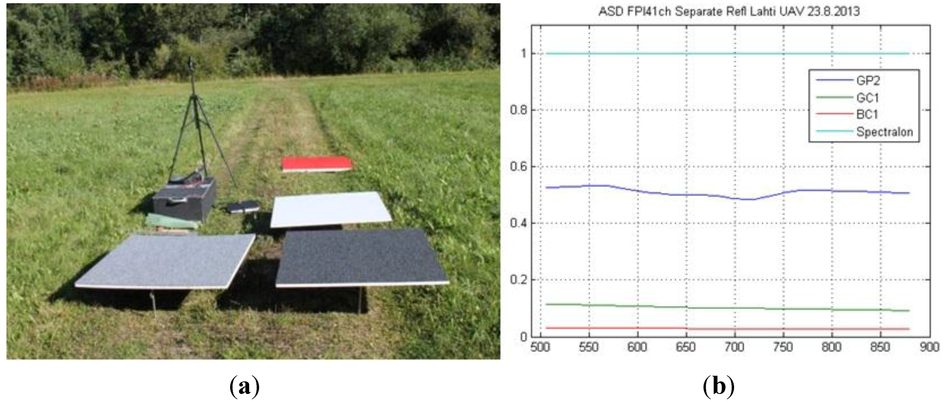
2.2. Remote Sensing Acquisition

For the empirical investigation, UAV-based data acquisition was carried out in the test areas of Kerinkallio and Mukkula on 23 August 2013. The dimensions of the areas were 260 m × 160 m and 180 m × 200 m, respectively. Weather conditions were windless during the flights; illumination conditions were sunny during the Mukkula flight and variable during the Kerinkallio flight. We used an octocopter-UAV, which was based on MikroKopter autopilot and Droidworx AD-8 extended frame and had a payload of 1.5 kg (Figure 1). The UAV was equipped with a stabilied camera mount of AV130 (PhotoHigher, Wellington, New Zealand), which compensates for tilts and vibrations around the roll and pitch directions.
The predominant instrument used in hyperspectral imaging was the FPI hyperspectral camera [35,36,37]. This technology provides spectral data cubes with area format and enables stereoscopic and multi-ray views of objects when overlapping images are used. However, due to the sequential exposure of the individual bands (0.075 s between adjacent exposures, 1.8 s during the entire data cube with 24 exposures), each band in the data cube has a slightly different position and orientation, which has to be taken into account in the post-processing phase. The sensor was used in a two-times binned mode, providing an image size of 1024 × 648 pixels with a pixel size of 11 μm and a focal length of 10.9 mm. The field of view (FOV) is ±18° in the flight direction, ±27° in the cross-flight direction, and ±31° at the format corner. Furthermore, an irradiance sensor based on Intersil ISL29004 photodetector is integrated to the camera to measure the wideband irradiance during each exposure [35,36,37,38]. A GPS receiver is used to record an exact time of the first exposure of each data cube. In order to capture high spatial resolution data, the UAV was also equipped with an ordinary RGB compact digital camera, Samsung NX1000. The camera has a 23.5 × 15.7 mm CMOS sensor with 20.3 megapixels, and a 16 mm lens.
Figure 1. UAV system for the field campaign (a). The cameras used in the study were the Fabry Pérot Interferometer (FPI) hyperspectral camera [37] (b) and red, green and blue (RGB) camera from Samsung (c).
Remotesensing 07 15467 g001
Table 3. Parameters of the unmanned airborne vehicle (UAV) flights on 23 August 2013 in the test areas. Flying altitude is from the ground level. f: forward overlap; s: side overlap; overlaps are for the nominal flying height of 90 m.
AreaCameraGSD (cm)Flying Alt. (m)Time (UTC + 3)Solar ElevationSun AzimuthExposure (ms)Overlap f; s (%)
MukkulaFPI9.055–9010:29–10:35 a.m.31.88130.06655; 55
MukkulaRGB2.455–9011:20–11:27 a.m.35.98143.97 70; 65
KerinkallioFPI9.070–901:48–1:55 p.m.40.01190.27855; 55
KerinkallioRGB2.470–901:10–1:17 p.m.40.35178.05 70; 65
Figure 2. The flight lines with UAV, sampling plots and reference target locations in Kerinkallio (a), and Mukkula (b).
Remotesensing 07 15467 g002
RGB and FPI cameras were operated from the UAV in separate flights in both areas, so there were four flights in total (Table 3, Figure 2). We used a flying altitude of 90 m from the ground level at the takeoff position, providing a nominal ground sample distance (GSD) of 9 cm for the FPI camera and 2.4 cm for the RGB-camera. In practice, the terrain height variation and the tree heights resulted in a large variation in the UAV to object distance: the flying height was 55–90 m and 70–90 m from the ground level in Mukkula and Kerinkallio, respectively, and 40–85 m and 55–85 m from the treetops, respectively. This provided GSDs of 4 cm to 8.5 cm at treetops for the FPI images, and 1.1 cm to 2.3 cm for the RGB images. Average speed of flights was approximately 5 m/s.
The FPI spectral camera was operated in the wavelength range of 500–900 nm. The number of spectral bands was originally 41. With spectral smile correction and band matching, the number of bands was reduced to 22. Full Width at Half Maximum (FWHM) of bands varied between 16 and 32 nm, depending on bands (for further details of a spectral settings, see Table 4). Exposure time was set to 6 ms in Mukkula and 8 ms in Kerinkallio (Table 3); our experiences have shown that these values provide good image quality in forested scenes in sunny illumination conditions.
Table 4. Settings of the FPI camera data capture: central wavelength (L0), full width of half maximum (FWHM), and temporal (dt) and spatial (ds) distance to the first exposure of the data cube.
L0 (nm): 516.50, 522.30, 525.90, 526.80, 538.20, 539.20, 548.90, 550.60, 561.60, 568.30, 592.20, 607.50, 613.40, 626.30, 699.00, 699.90, 706.20, 712.00, 712.40, 725.80, 755.60, 772.80, 793.80, 813.90
FWHM (nm): 20.00, 16.00, 22.00, 18.00, 24.00, 20.00, 18.00, 24.00, 16.00, 32.00, 22.00, 28.00, 30.00, 30.00, 18.00, 30.00, 28.00, 22.00, 28.00, 22.00, 28.00, 32.00, 30.00, 30.00
dt to first exposure (s): 0.825, 1.5, 0.9, 1.2, 0.975, 1.275, 1.35, 1.05, 1.65, 0.075, 0.15, 0.225, 0.3, 0.375, 1.65, 0.525, 0.6, 1.275, 0.675, 1.35, 0.825, 0.9, 0.975, 1.05
ds (computational) to first exposure (m): 4.1, 7.5, 4.5, 6.0, 4.9, 6.4, 6.8, 5.3, 8.3, 0.4, 0.8, 1.1, 1.5, 1.9, 8.3, 2.6, 3.0, 6.4, 3.4, 6.8, 4.1, 4.5, 4.9, 5.3
Figure 3. The radiometric reference targets and Avantes spectrometer in the campaign area (a). The reflectances of reference panels based on Avantes measurements during the campaign (b).
Remotesensing 07 15467 g003
We installed reflectance reference targets of a size of 1 m x 1 m and approximate reflectance of 0.03, 0.09 and 0.50 on the field nearby the study sites in order to transform the image data to reflectance. We carried out insitu reflectance measurements using the Avantes AvaSpec 3648 hand held spectrometer (Avantes BV, Apeldoorn, The Netherlands) (Figure 3).
We used the national airborne scanning (ALS) data by the National Land Survey of Finland (NLS) for the geometric reference [39]. The minimum point density of the NLS’s ALS data is half a point per square metre, and the elevation accuracy of the points in well-defined surfaces is 15 cm. The horizontal accuracy of the data is 60 cm. The point cloud has an automatic ground classification. The ALS data used in this study was collected in April 2009. The Matlab software (The MathWorks Inc., Natick, MA, USA) was used to create a DSM from the ALS point cloud using “first” and “only” pulses. The ALS DSM was interpolated to the same grid spacing as in photogrammetric DSMs: 10 cm in Kerinkallio and 12 cm in Mukkula. The digital elevation models (DEM) provided by the NLS were used as ground elevation data. The DEM is derived from the ALS point cloud and has an average vertical accuracy of 0.3 m and spatial resolution of 2 m.

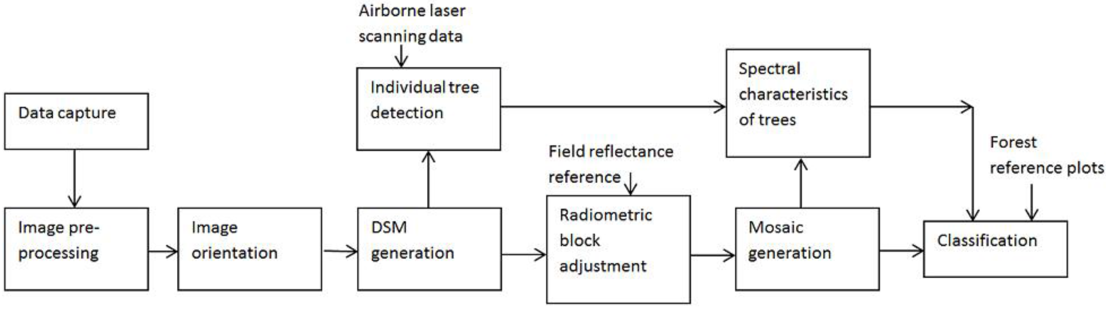
2.3. The Workflow for Analysis

Hundreds of small-format UAV-images were collected to cover the areas of interest. Rigorous pre-processing was required for the data in order to derive quantitative information from the imagery (Figure 4) (see details in [35,37]). The workflow of the analysis was as follows:
  • System corrections of the images using laboratory calibrations, spectral smile correction, and dark signal corrections
  • Determination of image orientations
  • Use of dense matching methods to create three dimensional (3D) geometric model of the object
  • Calculation of a radiometric imaging model to transform the digital numbers (DNs) to reflectance
  • Calculation of the reflectance output products: spectral image mosaics and bidirectional reflectance factor (BRF) data
  • Identification of individual trees
  • Spectral feature extraction for each tree
  • The final classification
In the following sections, we will describe the radiometric processing steps (1, 4, 5), geometric processing steps (2, 3) and further steps of tree identification (6), feature extraction (7) and classification (8) in more detail.
Figure 4. Data processing chain from the data capture to the classification.
Remotesensing 07 15467 g004

2.4. Geometric Processing

Geometric processing included two tasks; determination of the orientations of the images and determination of the 3D shape of the object by dense image matching. Our approach was to carry out an integrated geometric processing with the RGB images and several bands of the FPI images. Integrated orientation provided several advantages: (1) High overlaps were obtained between the images in the block (in individual blocks the overlaps were quite low), (2) the RGB images had better spatial resolution that improved the accuracy of matching based orientation, and, furthermore, (3) this approach enabled accurate extraction of image positions from the autopilot GPS-trajectory; the FPI images had accurate GPS time stamps, whereas timing information of the RGB camera was not accurate. The image orientations and DSMs were determined using Agisoft PhotoScan Professional commercial software (AgiSoft LLC, St. Petersburg, Russia). PhotoScan performs photo-based 3D reconstruction based on feature detection and dense matching, and its excellent performance has been validated in previous studies [40,41]. The bands of the FPI images that were not included in the orientation processing were matched to the oriented bands using band matching.
In the integrated orientation processing, there were a total of 357 images for the Kerinkallio block and 291 images for the Mukkula block (RGB images and two FPI image bands from the data cubes before smile correction; the central wavelength (L0) and the time difference to the first exposure of the data cube (dt): L0 = 546.60 nm, dt =1.05 s; L0 = 619.50 nm, dt = 0.375 s). In the PhotoScan processing, the quality was set to “high”; the settings for the number of key points per image were 40,000 and for the final number of tie points per image 1000; an automated lens calibration was performed simultaneously. The initial processing provided image orientations and a sparse point cloud in the internal coordinate system of the software. For the data, an automatic outlier removal was performed on the basis of the re-projection error (10% of points with the largest errors were removed). Some points were also removed manually from the sparse point cloud (points on the sky and below the ground). In order to transform the image orientations to the ETRS-TM35FIN coordinate system, the GPS-coordinates and the barometric height data of the FPI images were used; they were interpolated from the flight trajectory of the autopilot, using the accurate timing information of the images. In the final adjustment, the standard deviation settings were 3 m for the exterior orientations and four pixels to the tie points. The outputs of the process were the image exterior orientations and the camera calibrations in the object coordinate system.
Dense point clouds were generated using RGB and FPI images simultaneously. The point cloud generation was carried out using two-times down-sampled images in the Kerinkallio dataset, and four-times down-sampled images in the Mukkula dataset. In both datasets, a moderate filtering was used to eliminate outliers, which allowed relatively high height differences for the dataset.
A band matching procedure was used for the bands that were not included in the orientation processing (Figure 5). Band matching was carried out using a feature-based matching algorithm, and an affine transformation was used to map the bands to the reference bands [37]. We used three bands (band 8: L0 = 550.60 nm; dt = 1.05 s, band 14: L0 = 626.3 nm; dt = 0.375 s, band 24: L0 = 813.90 nm; dt = 1.05 s) as reference bands, corresponding the bands that were oriented by the PhotoScan. Analysis of the data cubes showed that the band matching was successful, excluding the bands 15 (L0 = 699.0 nm; dt = 1.65) and 18 (L0 = 712.0 nm; dt = 1.275) that were temporally the most distant from the used reference bands. These bands could be excluded from the analysis, because the data included other bands that were spectrally close to these bands (spectral distance was under 1 nm). Finally, there were a total of 22 bands to be used in the analysis.
Figure 5. Image data used in the study: (a) single band of the hyperspectral image data; (b) three band composition of hyperspectral images without band matching (23, 9 and 2); (c) band matched image; and (d) color image with red, green and blue (RGB) bands.
Remotesensing 07 15467 g005

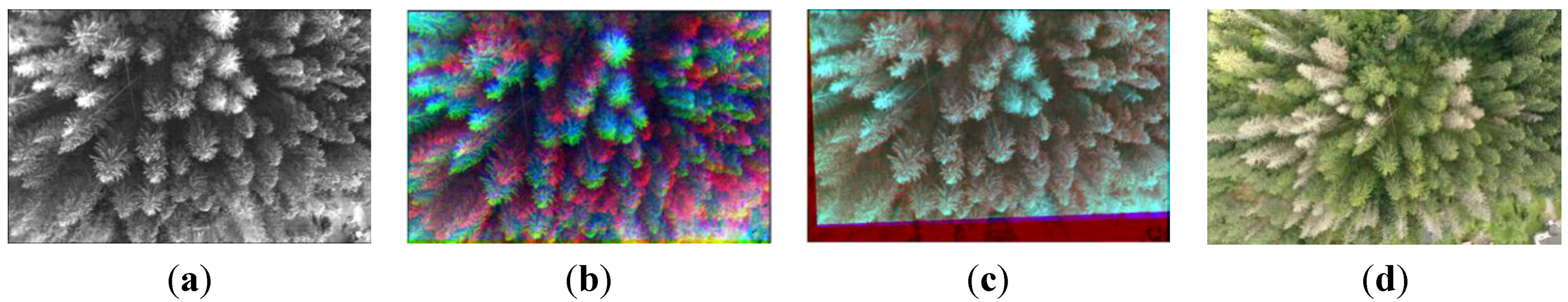
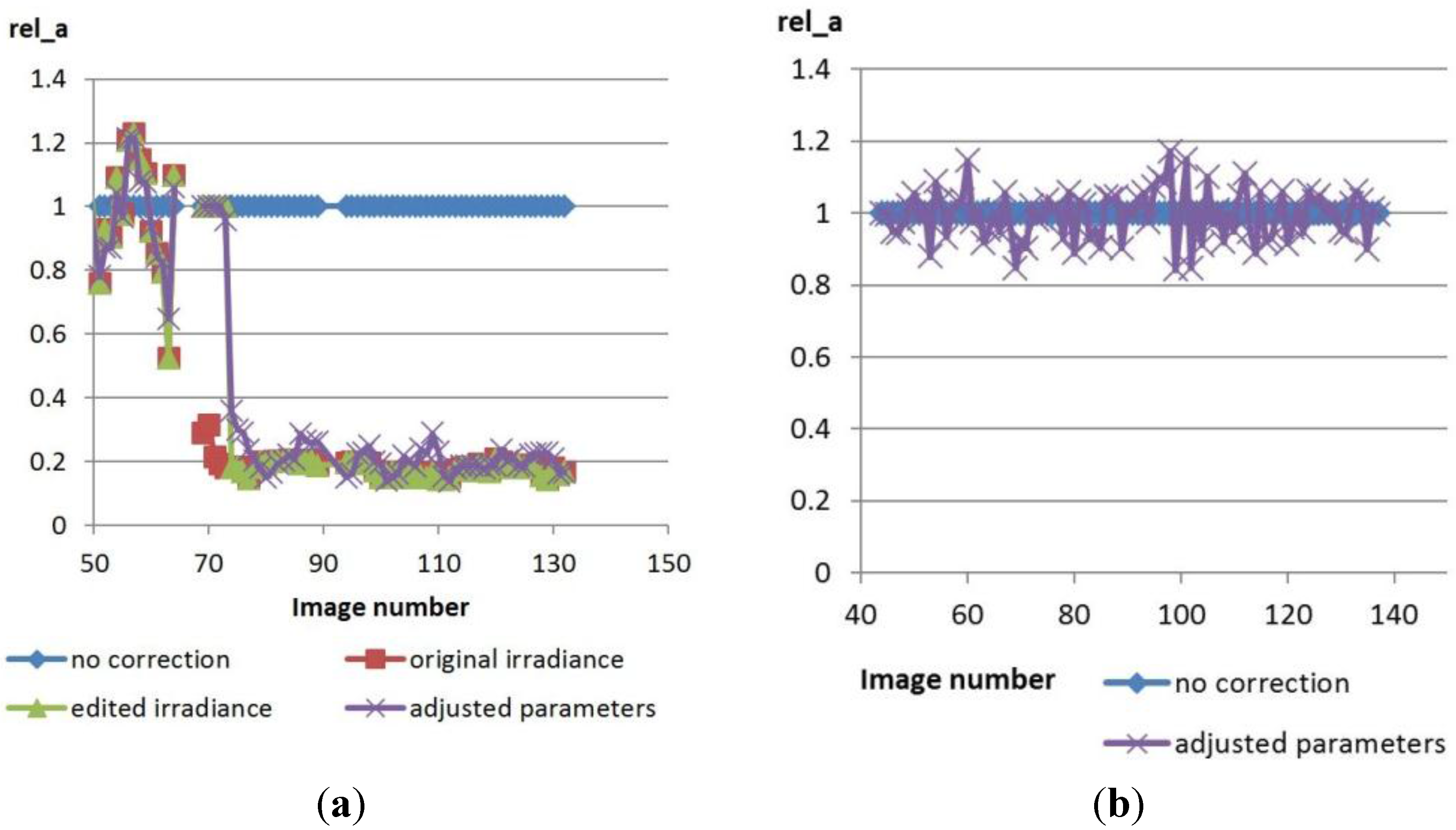
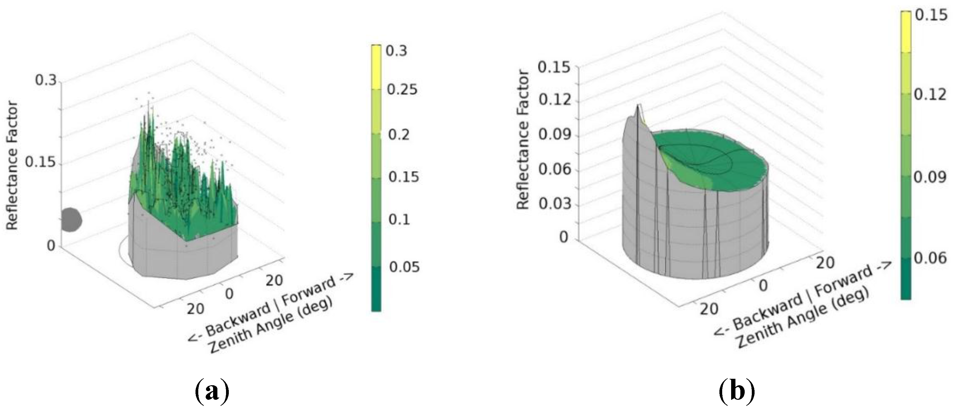
2.5. Radiometric Processing and Mosaic Generation

Laboratory calibration and spectral smile correction were carried out using methods developed by VTT (VTT Technical Research Centre of Finland Ltd) [35]. We used the empirical line method [42] to calculate the transformation from reflectance to DNs for each channel
DN = aabs Refl + babs
where aabs and babs are the parameters of the transformation. Three reference reflectance panels in the test area were used to determine the parameters; panel with average reflectance 0.5 was saturated in bands with visible light, therefore, we used for these bands only two of the panels.
Because of variable weather conditions and other radiometric phenomena, additional radiometric corrections were necessary in order to make image mosaics uniform. To solve this problem, a radiometric block adjustment method was used [37]. The basic principle of the method is to use the grey values (DN) of the radiometric tie points in the overlapping images as observations and to determine the model parameters describing the differences in DNs in different images (the radiometric model) indirectly via the least squares principle. The model for reflectance was
Rjkir,φ) = (DNjk / arel_jbabs) / aabs
where Rjkir,φ) is the bi-directional reflectance factor (BRF) of the object point, k, in image j; θi and θr are the illumination and reflected light (observation) zenith angles, φi and φr are the azimuth angles, respectively, and φ = φr − φi is the relative azimuth angle; aabs and babs are the parameters for the empirical line model for transforming the reflectance to DN and arel_j is the relative correction parameter with respect to the reference image. The parameters used can be selected according to the demands of the dataset in consideration.
In this study, the arel_j was based on the measurement by the irradiance sensor, and it was enhanced in the radiometric block adjustment. The correction factor based on irradiance measurement by the Intersil photodetector was
arel_j =Ej/Eref
where Ej and Eref are the irradiance measurements during the acquisition of image j and reference image ref.
The reflectance can be utilized either in the directional mode (BRF) or in the non-directional mode; in the latter case, quantity Rjk is used in Equation (2). More details of radiometric block adjustment are given in [37,38]. Finally, we calculated ortorectified reflectance mosaics with a GSD of 0.10 m in Kerinkallio and with GSD of 0.12 m in Mukkula by utilizing the DSMs, orientation information and the radiometric model.

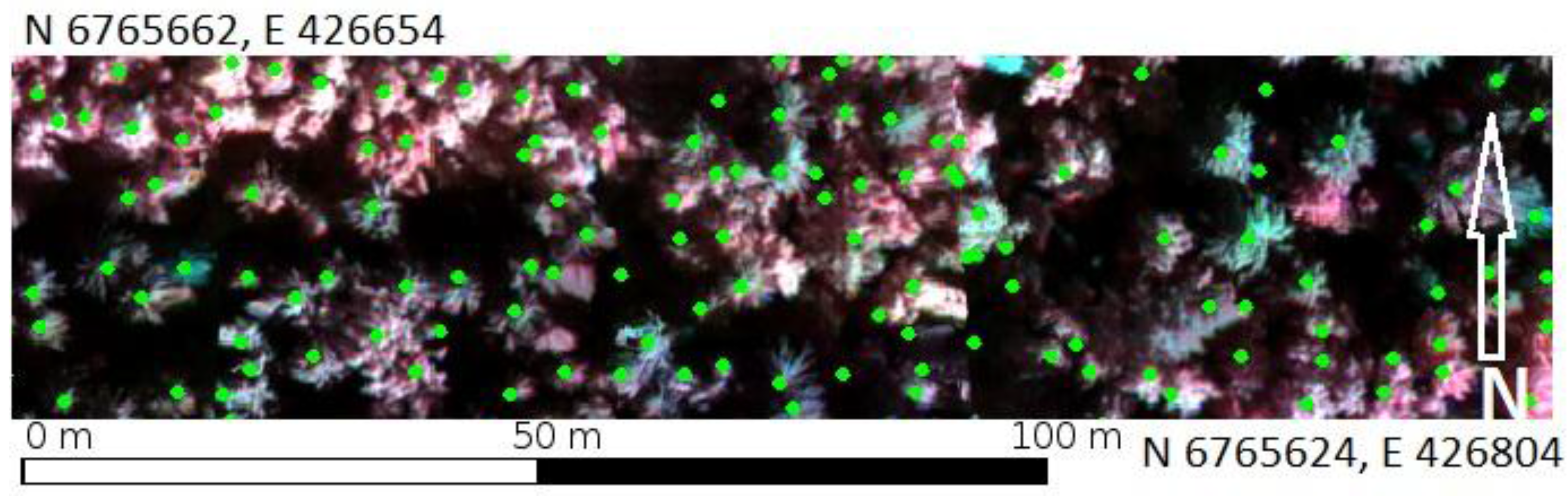
2.6. Individual Tree Detection

DSMs with a spatial resolution of 0.2 m, generated by dense matching, were utilized in the tree detection process. The DSMs were first transformed into canopy height models (CHM) by normalizing the heights with the ground elevation from the DEM provided by the NLS. Individual tree crowns were delineated from the CHMs with watershed segmentation [43,44]. The delineation process included smoothing the CHMs using 3 × 3 pixel mean filter. As the small-scale height variation of the original CHMs was high, the filtering was repeated eight times. The treetops were located by inverting the filtered CHMs and detecting the local minima (i.e., seed pixels). The crown segments were formed around the treetops by adding the neighboring pixels with same or higher height value to the segment region.

2.7. Spectrum and Feature Extraction

Because of the small GSD of 10 cm and 12 cm, there were many pixels related to each tree. This differs from the classical situation with hyperspectral imaging, with GSDs of larger than 50 cm, and only a few pixels for each tree. Our approach was to calculate a single spectral feature for each individual tree. We used a circular window with approximately 1 m diameter centered in the tree to calculate tree spectra. We visually confirmed that the coordinates of the trees matched the correct trees in the images. Small systematic shifts of 1 to 10 m for the entire group of treetops in each sample plot were necessary to align the field data with the images. Potential causes for the mismatches could be an inaccuracy of the GPS measurements for the centers of the sample plots during the field survey or geometric errors in the image mosaics. Our field check confirmed that the image coordinates of reference trees corresponded to the same trees on the ground.
We used either the average reflectance value of the window or the average of the six brightest pixels in the window. The latter approach was of interest, since the arithmetic mean might not be the ideal feature because of the large number of shadow pixels in the window. A similar approach has also been used in [24] for identifying air-pollution-based damage in Norway spruces.
Different sets of features were used in the analysis:
  • The original 22-band spectra.
  • Three different normalized channel ratios (indices) were computed using the reflectance (R) of two bands with wavelengths λ1 and λ2.
Index = (Rλ1Rλ2)/(Rλ1 + Rλ2)
One of them was the normalized difference vegetation index (NDVI), which is based on the spectra of near-infrared (NIR) and red channels; the other two were based on NIR and red edge bands and on visible bands. The bands used in the channel ratios were selected based on the analysis of variance (ANOVA) [45] to obtain knowledge on the differences of spectrums between various crown color classes (Section 3.4). This provided a three dimensional feature space.

2.8. Classification

Classification was done using the k-nearest neighbor classifier (k-NN), which is a supervised machine-learning technique [46]. Field observations of the tree health based on the color of tree crowns were used as a training set to classify all the trees in the research area. We used different values of k based on the amount of trees in the training data. The classifier was used for the entire spectra and for normalized ratios of bands. The leave-one-out cross validation technique was applied to assess performance of the k-NN classifier. Based on this method, we calculated the confusion matrix, Cohen’s kappa value (ϰ) [47], the producer’s, user’s and overall accuracies.

3. Results

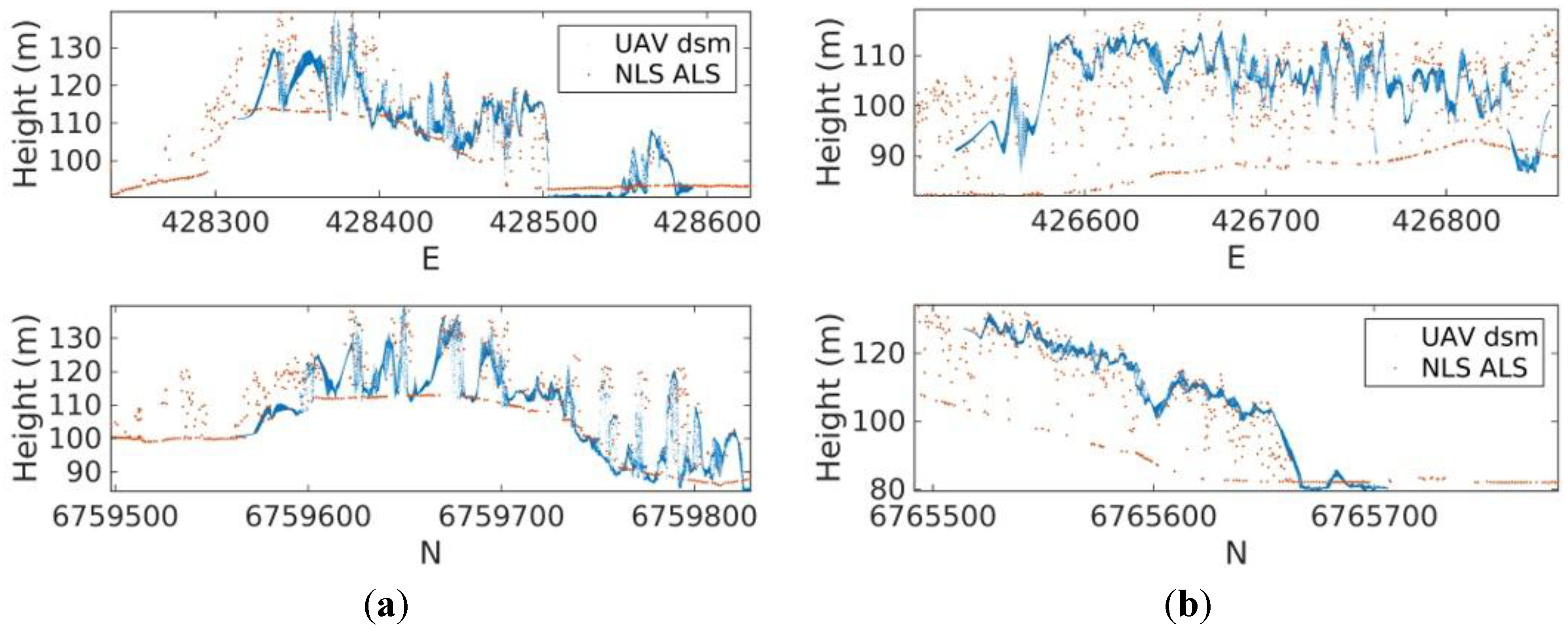
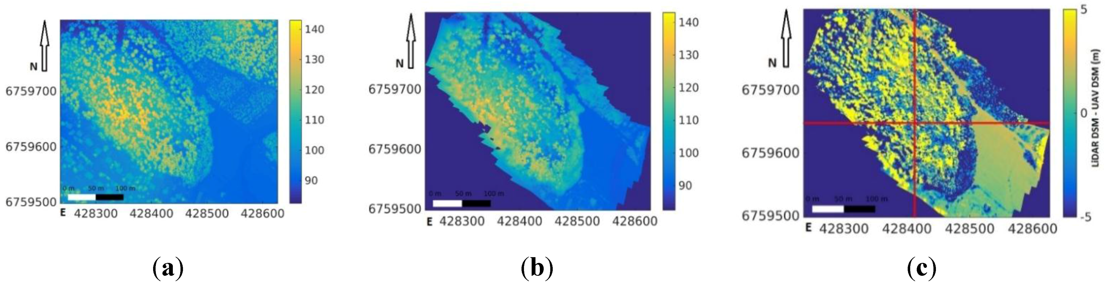
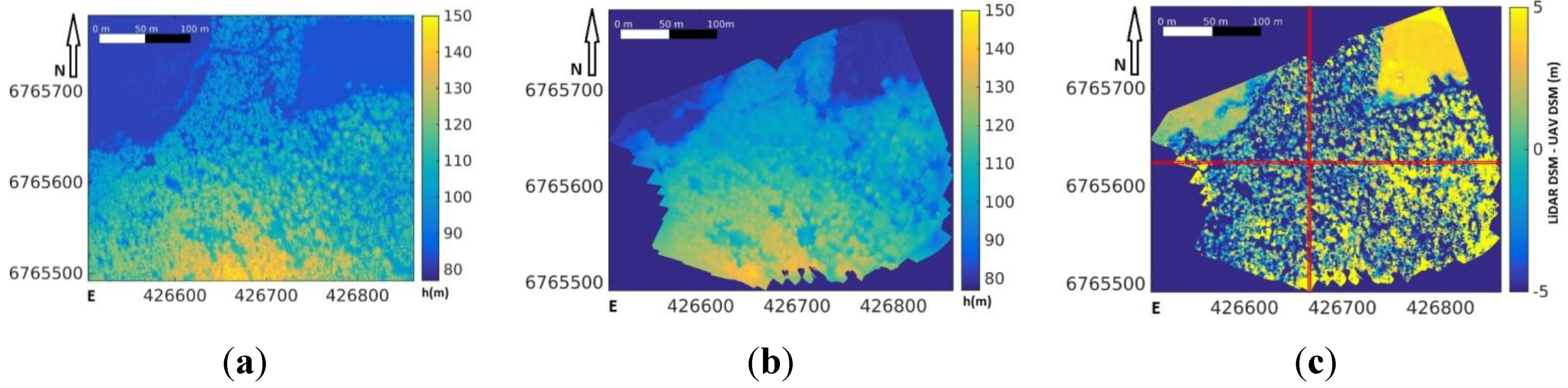
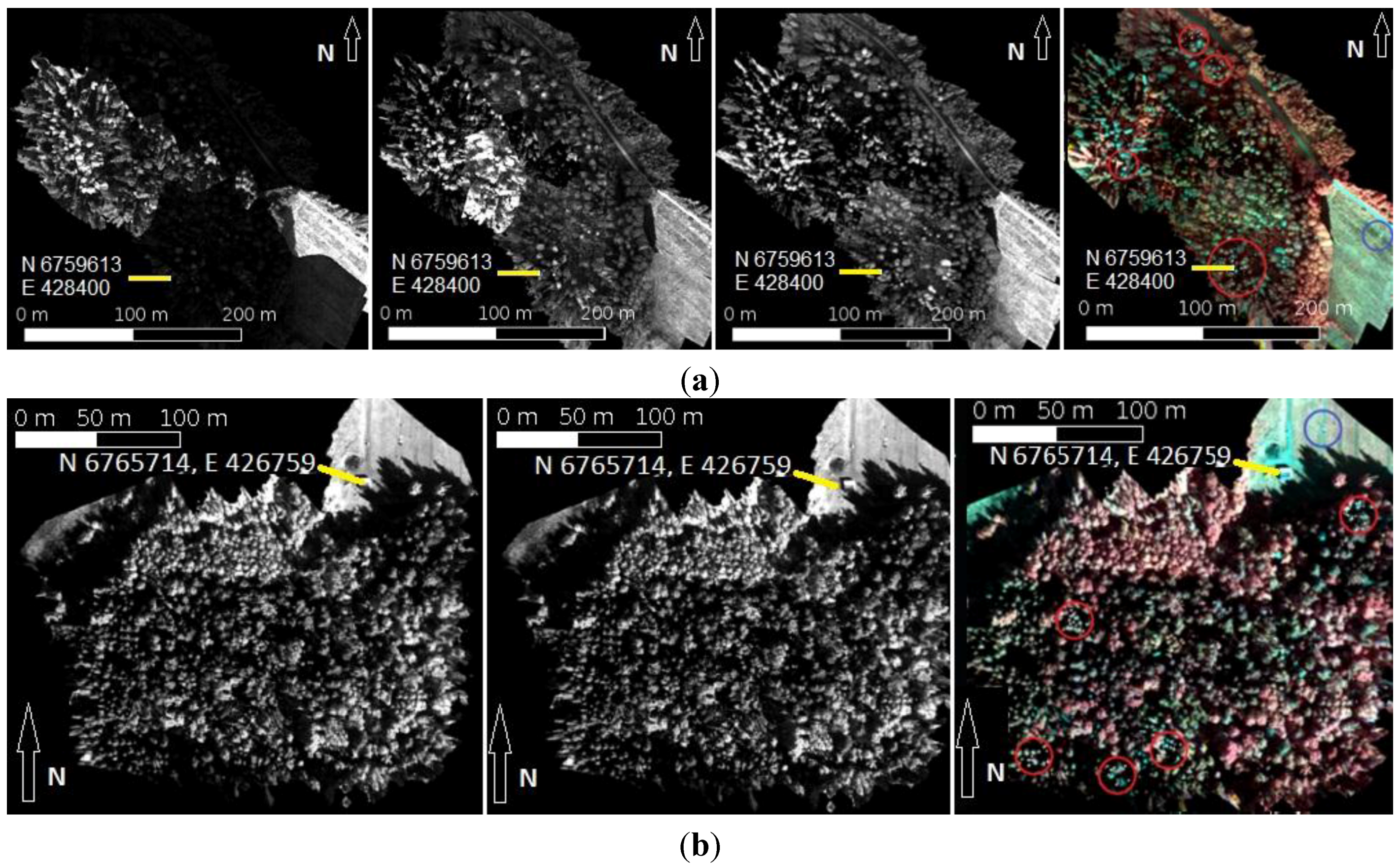
3.1. Geometric Processing

The geometric processing was successful for both datasets. The re-projection errors were approximately 0.4–0.5 pixels, and the root mean square error (RMSE) values of the GPS position residuals were at the level of 1–2 m (Table 5). In Mukkula, orientation was successful for all the images; in Kerinkallio, orientation failed on 8 images out of 365 images. These results indicated successful georeferencing. The number of generated points was 29 million in Kerinkallio and 3.5 million in Mukkula; the point densities were 424 and 71 points per m2, respectively. The difference in point density was due to the different resolution of images used in the point cloud generation (down-sampling was 2 times for Kerinkallio and 4 times for Mukkula).
Table 5. Statistics of the block adjustment calculation. Number of images, flying height (FH), number of tie points, re-projection error, RMSE at GPS-coordinates and the point density of the dense point cloud.
AreaN ImagesFH (m)Tie PointsReprojection Error (pix)GPS RMSE X; Y; Z (m)Point Density (Points per m2)
Kerinkallio3579075,0080.5050.989; 0.900; 0.875423.91
Mukkula2919076,7000.3531.031; 1.946; 0.38670.64
The DSMs from the UAV-photogrammetry and the NLS ALS data from the same location were compared visually. Profiles in latitude and longitude directions with 2 m width were plotted in 27–38 m intervals. For each area, 10 equally spaced profiles were plotted in both north and east directions. The profiles showed a good planar accuracy between the point clouds: visible treetops were mainly well aligned. The vertical accuracy of the generated DSM was not as good as the planar accuracy. Evaluation of the vertical accuracy was difficult because of the differences in the point clouds measured by photogrammetry and ALS. The photogrammetric point cloud had more upper canopy points and less ground hits compared to the ALS point cloud. The dense UAV-surface had the same form as the ALS-surface, but the levels were slightly different (Figure 6 and Figure 7). The differences in the densities and a large timespan between acquisitions of the point clouds also had an effect on the visual inspection of the point cloud alignment. In the central areas of the block, the absolute height accuracy was at the level of 1–2 m, with respect to the ALS DSM; in the block borders, the differences were larger due to the weakening of the block structure (Figure 8). The internal, relative accuracy of the point cloud can be expected to be on the level of GSD based on the re-projection error statistics (Table 5) as well as based on the systematic nature of the difference of the ALS and photogrammetric DSMs (Figure 8).
Figure 6. (a) Interpolated airborne laser scanning (ALS) first pulse digital surface model (DSM); (b) dense unmanned airborne vehicle (UAV) DSM; and (c) difference between DSMs ALS-UAV for the area in Kerinkallio.
Remotesensing 07 15467 g006
Figure 7. (a) Interpolated ALS first pulse DSM; (b) dense UAV DSM; and (c) difference between DSMs ALS-UAV.
Remotesensing 07 15467 g007
Figure 8. Example profiles from locations marked with red lines in Figure 6 and Figure 7 for (a) Kerinkallio and (b) Mukkula.
Remotesensing 07 15467 g008

3.2. Radiometric Processing

Image mosaics before radiometric corrections showed that the Kerinkallio dataset included many dark images because of clouds and varying illumination conditions (Figure 9a, leftmost). We used the irradiance sensor integrated to the FPI-camera and the radiometric block adjustment to eliminate the effects of changes of illumination. First, we used directly the irradiance data to calculate arel_j (Figure 10a, original irradiance). This correction caused some parts of the mosaic to become too light (Figure 9a, 2nd), which was due to the fact that the timing of the shadow by a cloud was different in the UAV than on the ground. We visually edited the irradiance data to correspond to the illumination at the object (Figure 10a, edited irradiance, images 69–74). A good radiometric uniformity was obtained for the mosaic when using the edited irradiance values as a priori values and calculating adjusted arel_j (Figure 9a, 3rd; Figure 10a, adjusted parameters) by the radiometric block adjustment. For the final calculation, we also eliminated eight partially cloudy images (images 65–68 and 90–93). It is worth noting that all the test sites were captured in cloudy conditions in Kerinkallio.
Figure 9. Impacts of different radiometric processing options in (a) Kerinkallio (channel 14) and (b) Mukkula (channel 18) datasets. From left: without any radiometric corrections, arel_j calculated from the original UAV irradiance measurements, arel_j calculated from the edited UAV irradiance measurements (only for Kerinkallio, see also Figure 10), final mosaic with three bands with arel_j based on radiometric block adjustment. The sample plots are marked with red circles and the reflectance panels are marked with blue circles in the rightmost mosaics.
Remotesensing 07 15467 g009
Figure 10. Values of parameter arel_j for each image on both blocks for channel 14 (L0 = 636.30 nm) (a) in Kerinkallio and (b) Mukkula.
Remotesensing 07 15467 g010
The Mukkula dataset provided uniform mosaic without corrections because of the stable and sunny weather conditions (Figure 9b). The radiometric block adjustment provided arel_j parameter values between 0.84 and 1.17, confirming that the variation of illumination conditions was small (Figure 10b). Mosaics were visually uniform both before and after the adjustment (Figure 9b).
Figure 11. Reflectance calculated in 3 m × 3 m windows of a regular grid of points in an 8 m × 8 m point interval presented as a function of relative azimuth angle and view zenith angle. (a) The raw reflectance observations and (b) the fitted bidirectional reflectance factor surface.
Remotesensing 07 15467 g011
We evaluated the impact of anisotropy by sampling reflectance values of the Mukkula dataset in a point grid with an 8 m point interval and plotting it as the function of the zenith and azimuthal angles of illumination and observation, and calculating a fitted bidirectional reflectance factor surface. This provided an averaged anisotropy for the forest area for the time of the campaign (Figure 11). The anisotropy was mostly less than 10% when limiting viewing zenith angles to <±15° from the nadir, which was the view zenith angle range used in the mosaicking; the high noise in the observations was due to the fact that we did not apply any point selection, thus the observations included both shaded and sun-illuminated pixels. The anisotropy was small in comparison to the actual variation of the reflectance and would have been challenging to determine using a small image block. We tested the bidirectional reflectance distribution function (BRDF) correction with the Mukkula dataset, but the results were not satisfactory; this was due to the fact that the current method has been developed for targets that do not have remarkable height differences with respect to the flying height, such as agricultural crops. The Kerinkallio data was captured in changing illumination conditions, making the BRDF correction even more complicated.

3.3. Individual Tree Detection

The watershed method performed well with the dense DSMs. We evaluated the tree extraction results in the study areas (Figure 12). These included 91 trees with a diameter at breast height over 25 cm. The accuracy of detection was 74.7%. Error of commission was 12 trees (13.1%).
Figure 12. Visualization of tree detection. Part of FPI mosaic, where detected trees are marked with green circles.
Remotesensing 07 15467 g012

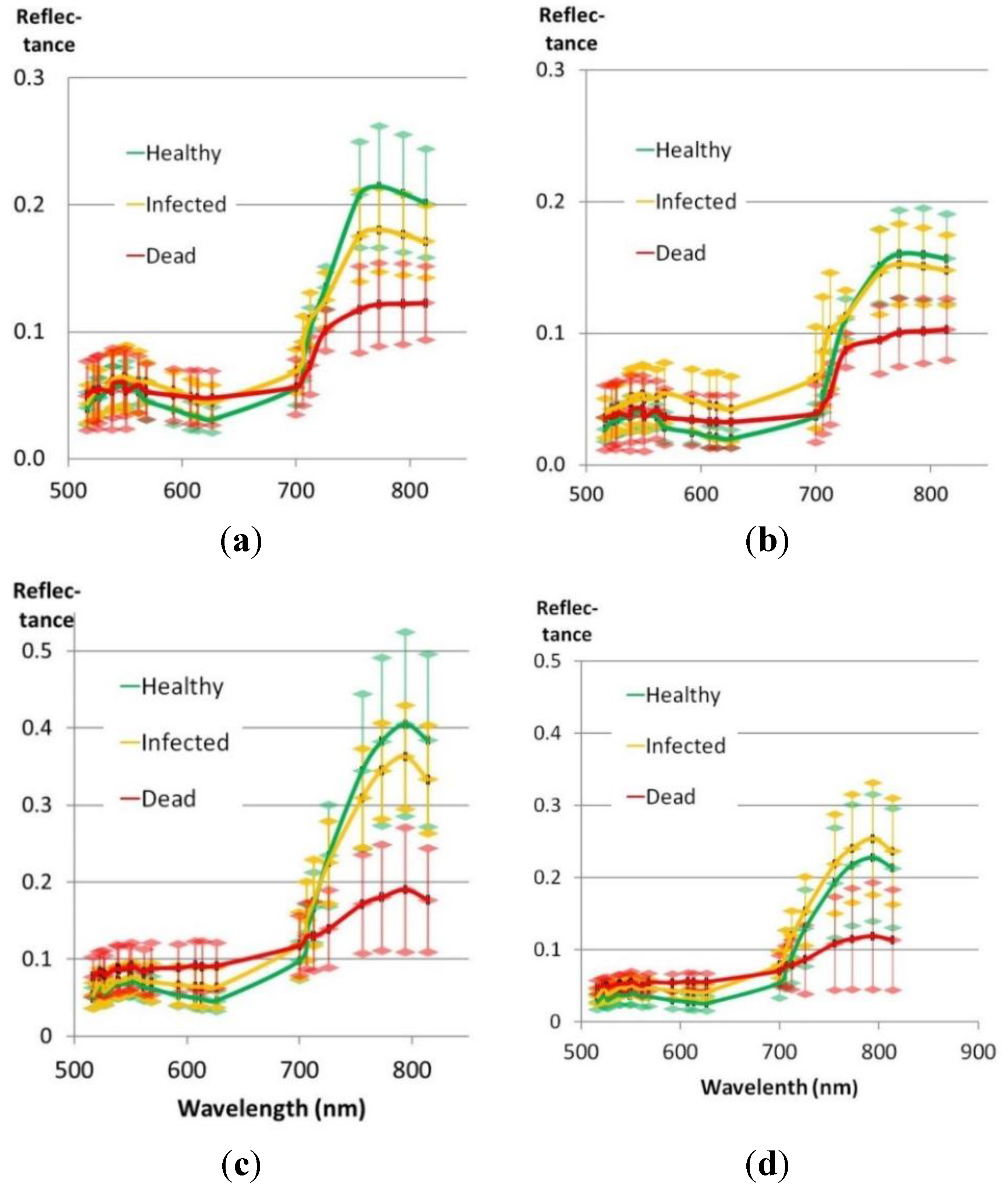
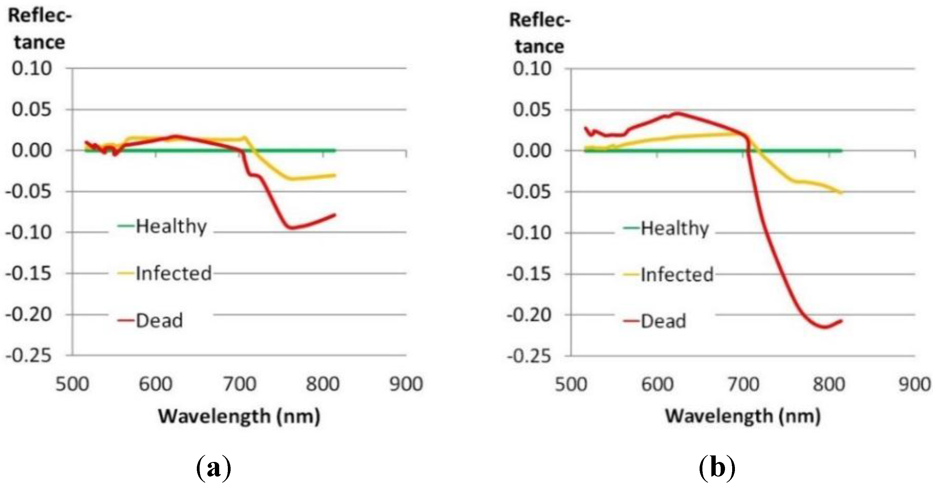
3.4. Spectral Data of Trees

A strategy of using an average of the six brightest pixels provided the most logical separation of the crown color classes when concerning the averaged spectra over the entire dataset. The infested and healthy classes that were separable when using the brightest pixels (Figure 13a,c) could not be separated when averages of all pixels were used (Figure 13b,d); the shadows caused this deterioration of the average spectra. Spectra of the dead trees differed significantly from the normal canopy reflectance spectra; the spectra were brighter in the visible wavelengths and darker in the NIR wavelengths. Only minor differences can be seen in the spectra of infested and healthy trees; in comparison to the healthy trees, the infested trees have a higher reflectivity in the red and green portions of the spectrum, and lower reflectivity in the NIR part of the spectrum. The levels of spectrums were higher for trees in Mukkula than for trees in Kerinkallio. Shapes of the spectra were, however, similar.
We analyzed the differences in the spectra of infested and dead spruces, with respect to healthy spruces, in order to select the most relevant bands for the vegetation index calculation (Figure 14). The first of the three best normalized channel ratios for the data from the ANOVA-analysis, according to Equation (4), corresponded to the NDVI using the channels with a central wavelength of λ1 = 793.8 nm and λ2 = 626.3 nm. The second was based on differences at the red-edge using the channels with a central wavelength of λ1 = 772.8 nm and λ2 = 725.8 nm. The third was based on visible light channels from green (λ1 = 550.6 nm) and red (λ2 = 626.3 nm) areas.
Figure 13. Average spectra with standard deviation bars of the healthy, infested and dead trees based on the image window, with a 1 m diameter in (a) Kerinkallio, average of six brightest pixels; (b) Kerinkallio, average of all pixels; (c) Mukkula, average of six brightest pixels; and (d) Mukkula, average of all pixels.
Remotesensing 07 15467 g013
Figure 14. Differences of spectrums of infested and dead spruces, with respect to healthy spruces in (a) Kerinkallio and (b) Mukkula.
Remotesensing 07 15467 g014

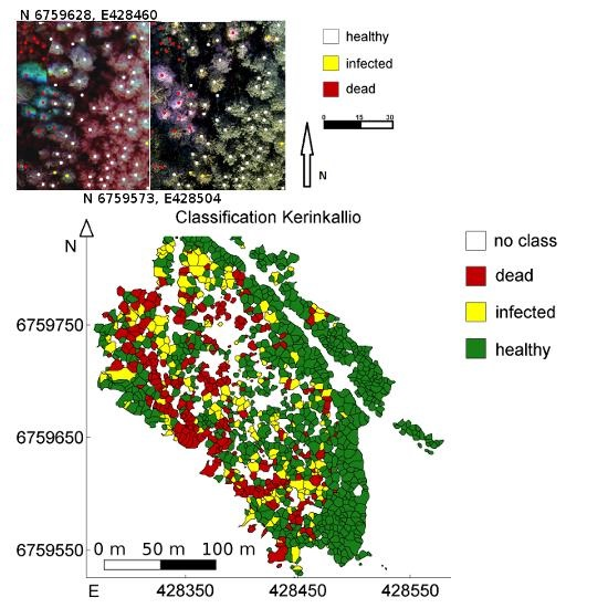
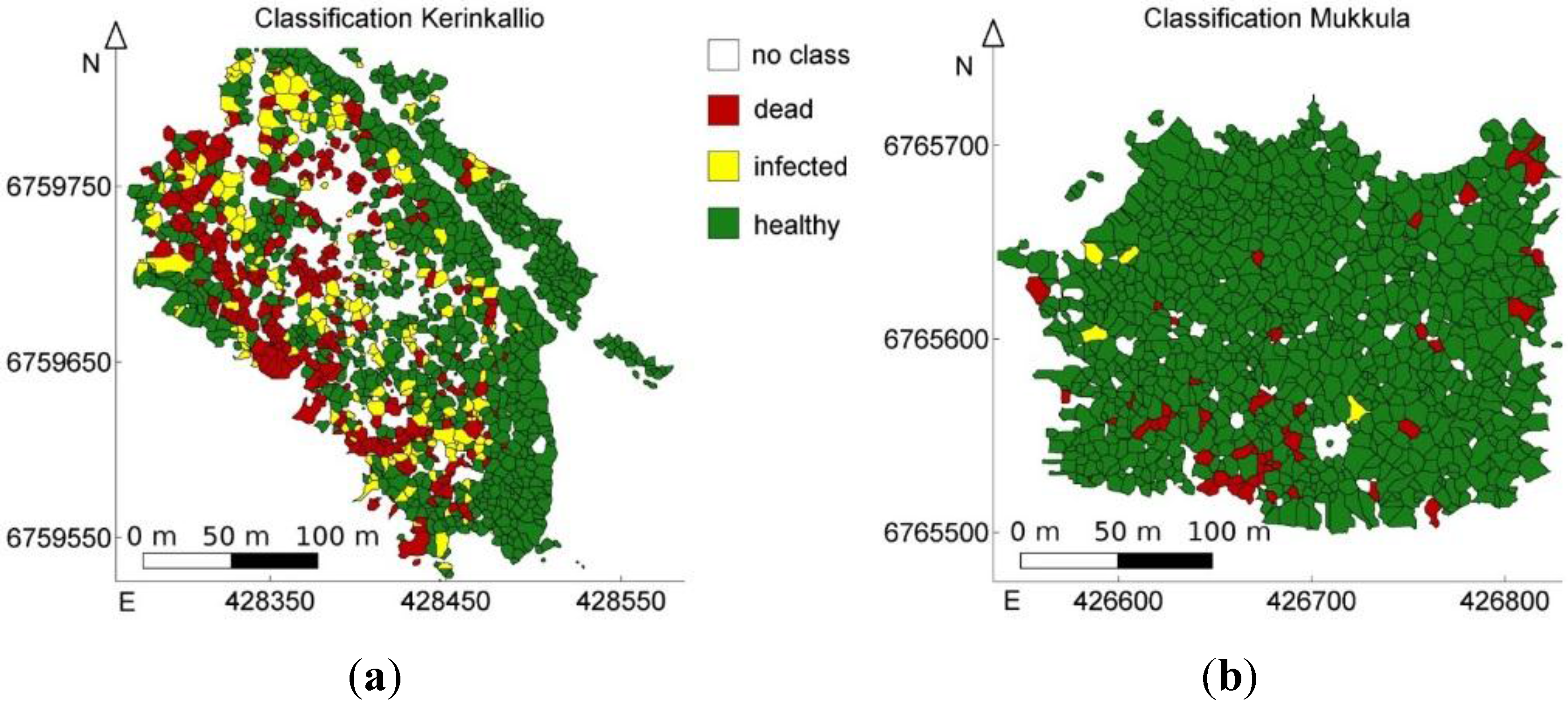
3.5. Classification Results

The classification of all three color classes (healthy, infested and dead) was challenging, due to the weak separation of the infested and healthy trees (Table 6). The indices provided slightly better accuracies than use of the full spectrum. When processing both areas simultaneously, the best overall accuracy was 76% (ϰ = 0.60) (78 samples in total). We also processed the Kerinkallio and Mukkula areas separately, although the number of the samples was low (39 in both datasets) (Table 6). The results were better for the Mukkula dataset; at best, the overall classification accuracy was 90% (ϰ = 0.79). For the Kerinkallio dataset, the best overall classification accuracy was 72% (ϰ =0.56). Potential explanation for better results of the Mukkula dataset could be the better imaging conditions during the data capture, which could have improved the separation of classes (see also Figure 14).
Table 6. Classification results for the case with three classes. N: number of samples; k: number of nearest neighbors used.
FeaturesAreaNkNumber of ClassesOverall Accuracy (%)KappaProducer’s Accuracy (%)
HealthyInfestedDead
Spectrumboth784375.640.3177.7846.6788.89
Indicesboth784375.640.6086.1133.3385.19
SpectrumKerinkallio393371.790.5650.0063.6488.89
IndicesKerinkallio393369.230.5350.0054.5588.89
SpectrumMukkula393379.490.5588.460.0088.89
IndicesMukkula393389.740.7996.1550.0088.89
Table 7. Classification results for the case with two classes. N: number of samples; k: number of nearest neighbors used.
FeaturesAreaNkNumber of ClassesOverall Accuracy (%)KappaProducer’s Accuracy (%)
HealthyInfestedDead
Spectrumboth784290.480.8191.67-88.89
Indicesboth784290.480.8094.44-85.19
SpectrumKerinkallio393289.290.7790.00-88.89
IndicesKerinkallio393285.710.7090.00-83.33
SpectrumMukkula393291.430.7892.31-88.89
IndicesMukkula393294.290.8596.15-88.19
Good separation could be obtained when using only two classes (healthy and dead) (Table 7). In the integrated classification of the both areas, the best result was obtained using vegetation indices; the overall accuracy was 90% (ϰ = 0.80; number of samples 78). When the two target areas were classified separately, the Mukkula area provided slightly better results. This dataset provided the best results with an overall accuracy of 94% (ϰ = 0.85); the producer’s accuracies were 96% for the healthy trees and 89% for the dead trees (number of samples 39 in each area).
Results of classification of all trees in the study areas are shown in Figure 15 and Figure 16.
Figure 15. Visualization of classification results using FPI color-infrared (a) and RGB (b) images on background.
Remotesensing 07 15467 g015
Figure 16. Tree level classification results in (a) Kerinkallio and (b) Mukkula. Segmentation is based on tree detection (Section 2.6).
Remotesensing 07 15467 g016

4. Discussion

4.1. Monitoring Infestation of Ips typographus

The climate change has already amplified the economic and ecological impacts of insect outbreaks. A rapid development of UAV-based remote sensing systems is enabling high-resolution and cost-efficient monitoring of forest environments. Hyperspectral sensors are powerful in detecting small anomalies in spectral characteristics of objects, i.e., tree crowns. In this study, we developed methodology for a UAV-based remote sensing system that utilizes photogrammetry and novel miniaturized hyperspectral sensor technology based on Fabry–Pérot interferometer (FPI). The data processing approach includes distinguishing spectral characteristics of individual crowns of trees at different stages of infestation. The method can be employed in monitoring changes in tree crown color by forest pest insects, such as bark beetles. The method is suitable when data in high detail is required and the target areas are relatively small. Practical implementations for this monitoring system include focal points of new insect-induced infestations and infestations in private-owned forests or urban forests and parks. We investigated the potential of the new method in detecting the infestation status of I. typographus at a tree-level in the Norway spruce, in urban forests of the city of Lahti. We captured image blocks in two sampling areas for assessing the performance of the method. The imaging system collected very high spatial-resolution image data; GSD was 2.4 cm for the RGB images and of 9 cm for the hyperspectral images at the nominal flying height of 90 m; at treetops, the GSDs were 1.1–2.3 cm and 4.0–9.5 cm with the RGB and hyperspectral images, respectively.

4.2. Geometric Performance

Geometric performance was consistent with the expectations. Image matching provided dense and detailed DSMs of the canopy surface with approximately 10 cm point density; the high quality could be expected based on previous studies with the Agisoft PhotoScan software [40,41]. The special feature of the processing was that the RGB images and several bands of FPI images were simultaneously used in the photogrammetric processing. Absolute height accuracy of the point clouds was on the level of 1–2 m. This is the expected level of absolute accuracy when using autopilot GPS and barometric data as a georeferencing reference. The internal, relative accuracy was estimated to be on the level of decimeter and thus feasible for branch level analyses as well as for derivation of accurate tree height information (if the terrain elevation could be obtained from the same DSM). The absolute accuracy can be improved by implementing more accurate GPS-positioning to the system, or by using ground control points as has been shown in previous studies [48,49]. Further aspects in the forest 3D characterization include the vagueness of tree crowns, and in windy weather, the tree movement will cause further deterioration in the reconstruction; these topics should be elaborated in further developments. This study proved for the first time the feasibility of the FPI technology in capturing 3D hyperspectral data in forested areas.

4.3. Radiometric Aspects

One of the advantageous features of the UAV systems is that the data capture can be carried out below clouds. However, this also sets challenges for the processing. We used UAV-based irradiance observations and a radiometric block adjustment to eliminate the radiometric non-uniformity of the image data [37]. The method compensated, at an average level, the illumination differences within image blocks; however, the spectra of individual trees were at different levels in the two datasets. The different conditions during the data acquisition were presumably the reason for the difference in the overall spectral levels of the two test blocks: the test plots in Kerinkallio were collected under variable illumination conditions, during partially cloudy weather, whereas during the flight of Mukkula, the weather was sunny and illumination was stable. The radiometric image corrections improved the results, but further studies are needed to normalize the datasets collected in sunny and cloudy weather if anticipating the analysis in a single classifier. We also pointed out the challenges in correcting the reflectance anisotropy effects in small image blocks collected in forested scenes. In future, it is necessary to investigate means to account for the BRDF effects in forested datasets, in particular, if multi-view reflectance observations are utilized in the interpretation task. It is obvious that approaches that differently consider the areas in sunshine or in various shadowed condition are needed [50,51]. Furthermore, for UAV remote sensing, the radiometric aspects need to be considered carefully [52,53]. One potential method for reducing the need for BRDF correction of image mosaics is to use high overlaps in the image capture and use the central parts of images in mosaicking. Furthermore, a stable illumination condition is recommended during the data capture if detailed spectral analyses are required.

4.4. Individual Tree Detection

The accuracy of delineating individual tree crowns from image-based point clouds has been a rare research topic. To our best knowledge, there are no publications concerning the issue in boreal forests. The tree delineation processes has been mainly developed for inventory related data retrieval, and detecting right number of trees has been the main issue, rather than the outline of a single tree crown. As the difference between ALS and image-based point clouds have been detected [54,55], we would like to point out that in the future, evaluation of the performance of image-based point clouds in tree delineation is an important line of studies that should be covered. When compared to ALS-based studies, the accuracy of detection reported in our study was roughly at the same level (e.g., [56,57]). However, only the biggest trees (DBH > 25 cm) were taken into account, which likely improves the reported detection rate.

4.5. Classification

The high-resolution data provided many possibilities for selecting features for the classification process. Our approach was to use an object based method and to calculate single features for each tree; another approach could have been to use all pixels of each tree, or even to take all pixels from each multi-view image to characterize the trees, or alternatively to use pixel based approach. The tree-level approach was feasible in the case of infestation by I. typographus, as the infestation usually leads to gradual, crown-wide symptoms until rapid death of the tree. The branch-level symptoms are rare [27]. Our results showed that the use of the brightest pixels in image windows, with a diameter of 1 m, provided better separation of the various classes than the use of averaged values; the latter quantity included both sunny and shaded pixels. In further studies, different features should be investigated. For example, Korpela et al. [50] used four different illumination classes, and used more pixels in the classification for each tree when investigating tree species classification. Puttonen et al. [51] used division into sunlit and shaded pixels to boost tree species classification with imagery that was not radiometrically corrected. Their method improved the classification by a few percent in comparison to their reference method.
The trees were classified as healthy (green), infested (yellow attack) and dead (grey). The class dead was clearly distinguishable from the healthy and infested classes. The classification into two classes provided good results, with an overall accuracy of 90% and Cohen’s kappa of 0.80 (78 samples). The separation of spectra of the infested and healthy trees was poorer. The overall accuracy was 76% and the kappa was 0.60, at best, when using three color classes (healthy, infested, and dead) (78 samples). The use of three spectral indices provided better results than the use of full spectra, which was consistent with the expectations; the neighboring channels are typically correlated and in the case, where training samples are limited in number, using too many features in classification is likely to result in poorer classification than with less features that were well selected [58]. The limitation of the experiment was that the training sample was very small. The class red attack was missing from the test area, and the number of trees with yellow attack was low. Furthermore, there were no observations of green attack, which was in practice impossible to identify with the survey methodology used in this study [20]. According our ground observations, green attack can be detected as a thin resin flow from the very first attack holes on a trunk, shifting a tree from a healthy class towards yellow attack. The trees with the very first infestation stage should be separated from healthy trees while collecting a ground reference for a further development of a methodology. This kind of more comprehensive approach could be carried out in unmanaged forested areas with all the stages of bark beetle attack available, such as in conservation areas or national parks.
It is worth noting that the UAV image datasets were collected in difficult illumination conditions, which probably caused some deterioration of the results. The classification accuracies are comparable to the previous studies in identifying different types of infestations with various sensors [17,24,25,27], but due to the small sample size, it is difficult to make further conclusions about the performance. The conclusion whether this accuracy is sufficient or not, is dependent on the application. However, the classification results can be considered to be very promising for further development of a methodology of distinguishing different phases of tree health and its depression. Important means to improve the identification of the dead trees and the yellow and red attack phases, in particular, will be to collect datasets in better imaging conditions, improve the radiometric processing, use more comprehensive training data, emphasize more in feature extraction and use more comprehensive classification method, such as the random forest based approaches. In contrary, we expect that the detection of the green attack might be extremely difficult [20]. Further interesting possibilities will be to add spectral data beyond the visible and near infrared wavelengths, in particular in short-wave infrared and thermal ranges [27,29]. Furthermore, integrating UAV measurements with satellite instruments, such as Landsat 8, might provide a deeper insight on the classification procedure, and might also offer possibility to extend the results to larger areas; this is interesting topic for future developments. It is also obvious that more information of the spectral characteristic of the green attack is needed, simultaneously with tree-wise ground truth [20]. Laboratory measurements could provide this information. A highly interesting approach would be to monitor areas with active bark beetle attacks with a high temporal resolution (e.g., weekly), using a hyperspectral UAV remote sensing system, which would provide observation data about the gradual spectral change within some weeks after a mass attack on Norway spruce trees.

4.6. Outlook

Timely managed actions are needed in forest protection against biotic disturbance agents, such as tree-killing bark beetle species. Several forest insect pests have benefitted from climate change and its drivers, such as heat spells and gales [1,11]. Traditional ground surveys are inadequate in locating the very first symptoms by phloem-consuming insect herbivores. The “infested” tree crown class showed promising results, particularly at the NIR area of the spectrum for further development of the method. Further improvements for the method could provide valuable information on the very initial green attack, indicating the risk in time. The information on incipient stress by pest insects is crucial for integrated pest management systems and forest health management planning. A UAV platform with hyperspectral sensor technology could provide the precise tools for the detection of crown discoloration, particularly in cumbersome and remote terrains [16]. In addition to bark beetles, this method can be applied for any other destructive biotic agents causing similar symptoms, e.g., the pine wood nematode (Bursaphelenchus xylophilus [59]). In addition, for commercial forests, the technology may be adopted for target areas under intensive survey needs, such as urban forest sites and parks. The developed UAV-based hyperspectral 3D remote sensing approach is feasible also for other applications in forestry where the tree color is important, such as tree species classification. The approach is cost-efficient in particular if spontaneous or high temporal frequency data capture is necessary.

5. Conclusions

Low-cost, miniaturized hyperspectral imaging technology is becoming available for small UAV platforms. This technology could be efficient for carrying out small-area inspections of anomalous reflectance characteristics of trees at a very high level of detail. In this investigation, a novel miniaturized hyperspectral frame imaging sensor was used to identify mature Norway spruce trees suffering from infestation by the invasive bark beetle I. typographus. We developed a processing approach for analyzing spectral characteristics for high spatial resolution photogrammetric and hyperspectral image data in a forested environment, as well as for identifying damaged trees. The point clouds measured, using dense image matching, enabled extraction of single trees with an accuracy of 74.7%. The results of classification of trees into healthy, infested and dead classes were promising. In particular, separation of healthy and dead trees provided a producer’s accuracy of 90% and a Cohen’s kappa of 0.80. The fine spatial resolution and combination of structure and hyperspectral information were unique approach. For the authors’ knowledge, this was the first study of using a hyperspectral imager in small UAV to identify bark-beetle-induced damage symptoms at a tree level. Furthermore, the results proved for the first time the feasibility of the Fabry-Pérot interferometer based hyperspectral imager in providing 3D hyperspectral information of tree canopies. We expect that the remote sensing technology developed here will be of great value in the future for identifying tree-wise damage, for investigating spectral characteristics of symptoms from early infestation until the death of the tree, as well as for other applications in forestry where the tree crown color is important, such as tree species classification.

Acknowledgments

This work was carried out in the MMEA research program, coordinated by Cleen Ltd (Helsinki, Finland) with funding from the Finnish Funding Agency for Technology and Innovation, Tekes. The project was also funded by the Niemi Foundation and the Maj and Tor Nessling Foundation. We wish to thank MSc Anna-Maaria Särkkä, head of the forestry unit in the city of Lahti for her cooperation. We would also like to thank Lauri Markelin for assistance in the fieldwork during the UAV campaign.

Author Contributions

Eija Honkavaara supervised the photogrammetric and remote sensing system and analysis development; Päivi Lyytikäinen-Saarenmaa supervised the field surveys. Roope Näsi took care of the post-processing chain and analysis of results; Teemu Hakala built the UAV data capture system and conducted the UAV data capture; Niko Viljanen carried out the photogrammetric processing; Paula Litkey developed the analysis method of DSMs; and Topi Tanhuanpää delineated the tree crowns from the point clouds. All authors contributed materials and analysis. Roope Näsi, Eija Honkavaara, Paula Litkey, Päivi Lyytikäinen-Saarenmaa, Minna Blomqvist and Topi Tanhuanpää wrote the manuscript. All authors commented on the manuscript and accepted the content.

Conflicts of Interest

The authors declare no conflict of interest.

References

  1. Seidl, R.; Schelhaas, M.J.; Lexer, M. Unraveling the drivers of intensifying forest disturbance regimes in Europe. Glob. Chang. Biol. 2011, 17, 2842–2852. [Google Scholar] [CrossRef]
  2. Lytikäinen-Saarenmaa, P.; Tomppo, E. Impact of sawfly defoliation on growth of Scots pine Pinus sylvestris (Pinaceae) and associated economic losses. Bull. Entomol. Res. 2002, 92, 137–140. [Google Scholar] [CrossRef] [PubMed]
  3. Björkman, C.; Bylund, H.; Klapwijk, M.J.; Kollberg, I.; Schroeder, M. Insect pests in future forests: More severe problems? Forests 2011, 2, 474–485. [Google Scholar] [CrossRef]
  4. Battisti, A.; Stastny, M.; Netherer, S.; Robinet, C.; Schopf, A.; Roques, A.; Larsson, S. Expansion of geographic range in the pine processionary moth caused by increased winter temperatures. Ecol. Appl. 2005, 15, 2084–2096. [Google Scholar] [CrossRef]
  5. Vanhanen, H.; Veteli, T.; Päivinen, S.; Kellomäki, S.; Niemelä, P. Climate change and range shifts in two insect defoliators: Gypsy moth and Nun moth—A model study. Silva Fenn. 2007, 41, 621–638. [Google Scholar] [CrossRef]
  6. Kurz, W.A.; Dymond, C.C.; Stinson, G.; Rampley, G.J.; Neilson, E.T.; Carroll, A.L.; Ebata, T.; Safranyik, L. Mountain pine beetle and forest carbon feedback to climate change. Nature 2008, 452, 987–990. [Google Scholar] [CrossRef] [PubMed]
  7. Jönsson, A.M.; Harding, S.; Krokene, P.; Lange, H.; Lindelöv, Å.; Okland, B.; Ravn, H.P.; Schroeder, L.M. Modelling the potential impact of global warming on Ips typographus voltinism and reproductive diapause. Clim. Chang. 2011, 109, 695–718. [Google Scholar] [CrossRef]
  8. Nabuurs, G.-J.; Lindner, M.; Verkerk, P.; Gunia, K.; Deda, P.; Michalak, R.; Grassi, G. First signs of carbon sink saturation in European forest biomass. Nat. Clim. Chang. 2013, 3, 792–796. [Google Scholar] [CrossRef]
  9. Bakke, A. The recent Ips typographus outbreak in Norway—Experiences from a control program. Holarct. Ecol. 1989, 12, 515–519. [Google Scholar] [CrossRef]
  10. Mezei, P.; Grodzki, W.; Blazenec, M.; Jakus, R. Factors influencing the wind—Bark beetles’ disturbance system in the course of an Ips typographus outbreak in the Tatra Mountains. For. Ecol. Manag. 2014, 312, 67–77. [Google Scholar] [CrossRef]
  11. Öhrn, P.; Långström, B.; Lindelöv, Å.; Björklund, N. Seasonal flight patterns of Ips typographus in southern Sweden and thermal sums required for emergence. Agric. For. Entomol. 2014, 16, 147–157. [Google Scholar] [CrossRef]
  12. Viiri, H.; Ahola, A.; Ihalainen, A.; Korhonen, K.T.; Muinonen, E.; Parikka, H.; Pitkänen, J. Kesän 2010 myrskytuhot ja niistä seuraavat hyönteistuhot. Metsätieteen Aikakauskirja 2011, 3, 221–225. [Google Scholar]
  13. Kärvemo, S.; Rogell, B.; Schroeder, M. Dynamics of spruce bark beetle infestation spots: Importance of local population size and landscape characteristics after a storm disturbance. For. Ecol. Manag. 2014, 334, 232–240. [Google Scholar] [CrossRef]
  14. Lausch, A.; Heurich, M.; Gordalla, D.; Dobner, H.-J.; Gwillym-Margianto, S.; Salbach, C. Forecasting potential bark beetle outbreaks based on spruce forest vitality using hyperspectral remote-sensing techniques at different scales. For. Ecol. Manag. 2013, 308, 76–89. [Google Scholar] [CrossRef]
  15. Schroeder, L.M. Colonization of storm gaps by the spruce bark beetle: Influence of gap and landscape characteristics. Agric. For. Entomol. 2010, 12, 29–39. [Google Scholar] [CrossRef]
  16. Faccoli, M. Effect of weather on Ips typographus (Coleoptera, Curculionidae) phenology, voltinism, and associated spruce mortality in the southeastern Alps. Environ. Entomol. 2009, 38, 307–316. [Google Scholar] [CrossRef] [PubMed]
  17. Ortiz, S.; Breidenbach, J.; Kändler, G. Early detection of bark beetle green attack using TerraSAR-X and RapidEye data. Remote Sens. 2013, 5, 1912–1931. [Google Scholar] [CrossRef]
  18. Wulder, M.A.; White, J.C.; Benz, B.; Alvarez, M.F.; Coops, N.C. Estimating the probability of mountain pine beetle red-attack damage. Remote Sens. Environ. 2006, 101, 150–166. [Google Scholar] [CrossRef]
  19. Göthlin, E.; Schroeder, L.M.; Lindelöw, Å. Attacks by Ips typographus and Pityogenes chalcographus on windthrown spruces (Picea abies) during the two years following a storm felling. Scand. J. For. Res. 2000, 15, 542–549. [Google Scholar] [CrossRef]
  20. Wulder, M.A.; Dymond, C.C.; White, J.C.; Leckie, D.G.; Carroll, A.L. Surveying mountain pine beetle damage of forests: A review of remote sensing opportunities. For. Ecol. Manag. 2006, 221, 27–41. [Google Scholar] [CrossRef]
  21. Kharuk, V.; Ranson, K.J.; Fedotova, E.V. Spatial pattern of Siberian silkmoth outbreak and taiga mortality. Scand. J. For. Res. 2007, 22, 531–536. [Google Scholar] [CrossRef]
  22. Coops, N.C.; Gillanders, S.N.; Wulder, M.A.; Gergel, S.E.; Nelson, T.; Goodwin, N.R. Assessing changes in forest fragmentation following infestation using time series Landsat imagery. For. Ecol. Manag. 2010, 259, 2355–2365. [Google Scholar] [CrossRef]
  23. Kantola, T.; Vastaranta, M.; Yu, X.; Lyytikainen-Saarenmaa, P.; Holopainen, M.; Talvitie, M.; Kaasalainen, S.; Solberg, S.; Hyyppa, J. Classification of defoliated trees using tree-level airborne laser scanning data combined with aerial images. Remote Sens. 2010, 2, 2665–2679. [Google Scholar] [CrossRef]
  24. Kantola, T.; Vastaranta, M.; Lyytikainen-Saarenmaa, P.; Holopainen, M.; Kankare, V.; Talvitie, M.; Hyyppa, J. Classification accuracy of the needle loss of individual Scots pines from airborne laser point clouds. Forests 2013, 4, 386–403. [Google Scholar] [CrossRef]
  25. De Somviele, B.; Lyytikäinen-Saarenmaa, P.; Niemelä, P. Stand edge effects on distribution and condition of Diprionid sawflies. Agric. For. Entomol. 2007, 9, 17–30. [Google Scholar] [CrossRef]
  26. Campbell, P.E.; Rock, B.N.; Martin, M.E.; Neefus, C.D.; Irons, J.R.; Middleton, E.M.; Albrechtova, J. Detection of initial damage in Norway spruce canopies using hyperspectral airborne data. Int. J. Remote Sens. 2004, 25, 5557–5584. [Google Scholar] [CrossRef]
  27. Fassnacht, F.E.; Latifi, H.; Ghosh, A.; Joshi, P.K.; Koch, B. Assessing the potential of hyperspectral imagery to map bark beetle-induced tree mortality. Remote Sens. Environ. 2014, 140, 533–548. [Google Scholar] [CrossRef]
  28. Lehmann, J.R.; Nieberding, F.; Prinz, T.; Knoth, C. Analysis of unmanned aerial system-based CIR images in forestry—A new perspective to monitor pest infestation levels. Forests 2015, 6, 594–612. [Google Scholar] [CrossRef] [Green Version]
  29. Calderón, R.; Navas-Cortés, J.A.; Lucena, C.; Zarco-Tejada, P.J. High-resolution airborne hyperspectral and thermal imagery for early detection of verticillium wilt of olive using fluorescence, temperature and narrow-band spectral indices. Remote Sens. Environ. 2013, 139, 231–245. [Google Scholar] [CrossRef]
  30. Garcia-Ruiz, F.; Sankaran, S.; Maja, J.M.; Lee, W.S.; Rasmussen, J.; Ehsani, R. Comparison of two aerial imaging platforms for identification of Huanglongbing-infected citrus trees. Comput. Electron. Agric. 2013, 91, 106–115. [Google Scholar] [CrossRef]
  31. Lisein, J.; Deseilligny, M.P.; Bonnet, S.; Lejeune, P. A photogrammetric workflow for the creation of a forest canopy height model from small unmanned aerial system imagery. Forests 2013, 4, 922–944. [Google Scholar] [CrossRef]
  32. Dandois, J.P.; Ellis, E.C. High spatial resolution three-dimensional mapping of vegetation spectral dynamics using computer vision. Remote Sens. Environ. 2013, 136, 259–276. [Google Scholar] [CrossRef]
  33. Puliti, S.; Ørka, H.O.; Gobakken, T.; Næsset, E. Inventory of small forest areas using an unmanned aerial system. Remote Sens. 2015, 7, 9632–9654. [Google Scholar] [CrossRef] [Green Version]
  34. Cajander, A.K. The theory of forest types. Acta For. Fenn. 1926, 29, 1–108. [Google Scholar]
  35. Mäkynen, J.; Holmlund, C.; Saari, H.; Ojala, K.; Antila, T. Unmanned aerial vehicle (UAV) operated megapixel spectral camera. Proc. SPIE 2011, 8186. [Google Scholar] [CrossRef]
  36. Saari, H.; Pellikka, I.; Pesonen, L.; Tuominen, S.; Heikkilä, J.; Holmlund, C.; Mäkynen, J.; Ojala, K.; Antila, T. Unmanned Aerial Vehicle (UAV) operated spectral camera system for forest and agriculture applications. Proc. SPIE 2011, 8174. [Google Scholar] [CrossRef]
  37. Honkavaara, E.; Saari, H.; Kaivosoja, J.; Pölönen, I.; Hakala, T.; Litkey, P.; Mäkynen, J.; Pesonen, L. Processing and assessment of spectrometric, Stereoscopic imagery collected using a lightweight UAV spectral camera for precision agriculture. Remote Sens. 2013, 5, 5006–5039. [Google Scholar] [CrossRef] [Green Version]
  38. Hakala, T.; Honkavaara, E.; Saari, H.; Mäkynen, J.; Kaivosoja, J.; Pesonen, L.; Pölönen, I. Spectral Imaging from UAVs under Varying Illumination Conditions. In Proceedings of International Society for Photogrammetry and Remote Sensing (ISPRS), Paris, France, 4–6 September 2013; pp. 189–194.
  39. National Land Survey of Finland Open Data License. Available online: http://www.maanmittauslaitos.fi/en/opendata/acquisition (accessed on 15 November 2015).
  40. Verhoeven, G. Taking computer vision aloft—Archaeological three-dimensional reconstructions from aerial photographs with PhotoScan. Archaeol. Prospect. 2011, 18, 67–73. [Google Scholar] [CrossRef]
  41. Eltner, A.; Schneider, D. Analysis of different methods for 3D reconstruction of natural surfaces from parallel-axes UAV images. Photogramm. Rec. 2015, 30, 279–299. [Google Scholar] [CrossRef]
  42. Smith, G.M.; Milton, E.J. The use of the empirical line method to calibrate remotely sensed data to reflectance. Int. J. Remote Sens. 1999, 20, 2653–2662. [Google Scholar] [CrossRef]
  43. Hyyppä, J.; Kelle, O.; Lehikoinen, M.; Inkinen, M. A segmentation-based method to retrieve stem volume estimates from 3-D tree height models produced by laser scanners. IEEE Trans. Geosci. Remote Sens. 2001, 39, 969–975. [Google Scholar] [CrossRef]
  44. Tanhuanpää, T.; Vastaranta, M.; Kankare, V.; Holopainen, M.; Hyyppä, J.; Hyyppä, H.; Alho, P.; Raisio, J. Mapping of urban roadside trees—A case study in the tree register update process in Helsinki City. Urban For. Urban Green. 2014, 13, 562–570. [Google Scholar] [CrossRef]
  45. Sokal, R.; Rohlf, F. Biometry: The Principles and Practice of Statistics in Biological Research; W.H. Freeman and Company: New York, NY, USA, 1995. [Google Scholar]
  46. Kotsiantis, S.B. Supervised machine learning: A review of classification techniques. Informatica 2007, 31, 249–268. [Google Scholar]
  47. Cohen, J. Weighted kappa: Nominal scale agreement provision for scaled disagreement or partial credit. Psychol. Bull. 1968, 70, 213–220. [Google Scholar] [CrossRef] [PubMed]
  48. Turner, D.; Lucieer, A.; Watson, C. An automated technique for generating georectified mosaics from ultra-high resolution unmanned aerial vehicle (UAV) imagery, based on structure from motion (SFM) point clouds. Remote Sens. 2012, 4, 1392–1410. [Google Scholar] [CrossRef]
  49. Vander Jagt, B.; Lucieer, A.; Wallace, L.; Turner, D.; Durand, M. Snow depth retrieval with UAS using photogrammetric techniques. Geosciences 2015, 5, 264–285. [Google Scholar] [CrossRef]
  50. Korpela, I.; Heikkinen, V.; Honkavaara, E.; Rohrbach, F.; Tokola, T. Variation and directional anisotropy of reflectance at the crown scale—Implications for tree species classification in digital aerial images. Remote Sens. Environ. 2011, 115, 2062–2074. [Google Scholar] [CrossRef]
  51. Puttonen, E.; Litkey, P.; Hyyppä, J. Individual tree species classification by illuminated-shaded area separation. Remote Sens. 2010, 2, 19–35. [Google Scholar] [CrossRef]
  52. Schaepman-Strub, G.; Schaepman, M.E.; Painter, T.H.; Dangel, S.; Martonchik, J.V. Reflectance quantities in optical remote sensing—Definitions and case studies. Remote Sen. Environ. 2006, 103, 27–42. [Google Scholar] [CrossRef]
  53. Honkavaara, E.; Arbiol, R.; Markelin, L.; Martinez, L.; Cramer, M.; Bovet, S.; Chandelier, L.; Ilves, R.; Klonus, S.; Marshal, P.; et al. Digital Airborne photogrammetry—A new tool for quantitative remote sensing?—A state-of-the-art review on radiometric aspects of digital photogrammetric images. Remote Sens. 2009, 1, 577–605. [Google Scholar] [CrossRef] [Green Version]
  54. Vastaranta, M.; Wulder, M.A.; White, J.; Pekkarinen, A.; Tuominen, S.; Ginzler, C.; Kankare, V.; Holopainen, M.; Hyyppä, J.; Hyyppä, H. Airborne laser scanning and digital stereo imagery measures of forest structure: Comparative results and implications to forest mapping and inventory update. Can. J. Remote Sens. 2013, 39, 382–395. [Google Scholar] [CrossRef]
  55. White, J.C.; Wulder, M.A.; Vastaranta, M.; Coops, N.C.; Pitt, D.; Woods, M. The utility of image-based point clouds for forest inventory: A comparison with airborne laser scanning. Forests 2013, 4, 518–536. [Google Scholar] [CrossRef]
  56. Persson, Å.; Holmgren, J.; Söderman, U. Detecting and measuring individual trees using an airborne laser scanner. Photogramm. Eng. Remote Sens. 2002, 68, 925–932. [Google Scholar]
  57. Koch, B.; Heyder, U.; Weinacker, H. Detection of individual tree crowns in airborne LiDAR data. Photogramm. Eng. Remote Sens. 2006, 72, 357–363. [Google Scholar] [CrossRef]
  58. Bishop, C. Pattern Recognition and Machine Learning; Springer: New York, NY, USA, 2006. [Google Scholar]
  59. Schröder, T.; McNamara, D.G.; Gaar, V. Guidance on sampling to detect pine wood nematode Bursaphelenchus Xylophilus in trees, wood and insects. EPPO Bull. 2009, 39, 179–188. [Google Scholar] [CrossRef]

