Continuous Change Detection and Classification Using Hidden Markov Model: A Case Study for Monitoring Urban Encroachment onto Farmland in Beijing

Abstract

In this paper, we propose a novel method to continuously monitor land cover change using satellite image time series, which can extract comprehensive change information including change time, location, and “from-to” information. This method is based on a hidden Markov model (HMM) trained for each land cover class. Assuming a pixel’s initial class has been obtained, likelihoods of the corresponding model are calculated on incoming time series extracted with a temporal sliding window. By observing the likelihood change over the windows, land cover change can be precisely detected from the dramatic drop of likelihood. The established HMMs are then used for identifying the land cover class after the change. As a case study, the proposed method is applied to monitoring urban encroachment onto farmland in Beijing using 10-year MODIS time series from 2001 to 2010. The performance is evaluated on a validation set for different model structures and thresholds. Compared with other change detection methods, the proposed method shows superior change detection accuracy. In addition, it is also more computationally efficient.

1. Introduction

The monitoring of land cover requires that changes be distinguished from stable land cover classes over time. Satellite image time series constantly provide global coverage of the earth’s surface information, which makes them perfect data sources for land cover change detection applications [1].

The general problem of change detection in monitoring time series has been extensively studies in the field of statistics [2] and data mining [3]. Autocorrelation techniques [4], segmentation algorithms [5], predictive approaches [6], statistical parameter change approaches [7], harmonic analysis [8], and subsequence clustering [9] are some of the time series change detection algorithms that have been successfully applied in the remote sensing field. Most of these methods aim at identifying changes from stable time series. However, they cannot provide detailed “from what, to what” information. A study on continuous change detection and classification (CCDC) was presented in [6], which used all available Landsat images acquired within the same area to estimate a time series model. The CCDC algorithm applies the model predictions for change detection and uses the model coefficients as the inputs for land cover classification. Because CCDC needs to estimate a model for each individual pixel, it is somewhat computational expensive and data storage costly.

Hidden Markov model (HMM) is a powerful statistical learning algorithm for temporal information modeling and forecasting, which has been successfully applied to various kinds of scientific and engineering change detection problems, including intrusion detection [10,11], video anomaly event detection [12,13], equipment fault diagnosis [14,15], and human daily activity monitoring [16,17]. Some researchers have introduced HMM to remote sensing change detection applications [18,19,20]. For example, Bouyahia et al. [21] used a hidden Markov chain model performed on a spatial sliding window to produce a change map from bi-date SAR images. Salberg and Trier [22] applied a two-state HMM to modeling time series of each pixel, each state in the model corresponded to a “forest” or “non-forest” type, and then detected forest changes from the subsequent state estimates. Mithal et al. [23] trained an HMM for land cover label sequences and used the model to relabel misclassified pixels. Ito et al. [24] proposed an HMM-based anomalous signal detection algorithm to predict the precursor of an earthquake.

In this study, we present a novel HMM-based continuous change detection and classification (HCCDC) algorithm that can provide detailed “from–to” change information. HCCDC works in a class-wise manner, without the need of constructing a separate model for each pixel. It is motivated by a simple idea. First, an HMM is learned for each land cover class. Then, for a particular pixel (its class at the initial time is known), likelihoods of the corresponding HMM on incoming time series will maintain relatively high values if its class is persistent. However, when change occurs, likelihoods are supposed to decline to rather low values. Therefore, by applying a temporal sliding window on incoming series and observing likelihood change over the windows, land cover change can be precisely detected. Finally, classification is made to provide land cover-land use conversion information.

For the validation of HCCDC, a case study in Beijing, China is provided. The encroachment of urban land onto farmland is one of the most pervasive forms of land cover change in Beijing. The proposed method is applied to monitoring farmland loss using 10-year MODIS time series from 2001 to 2010. The results are evaluated on a validation set and compared with the outcomes of the other two contemporary change detection methods.

2. Study Area and Data

2.1. Study Area

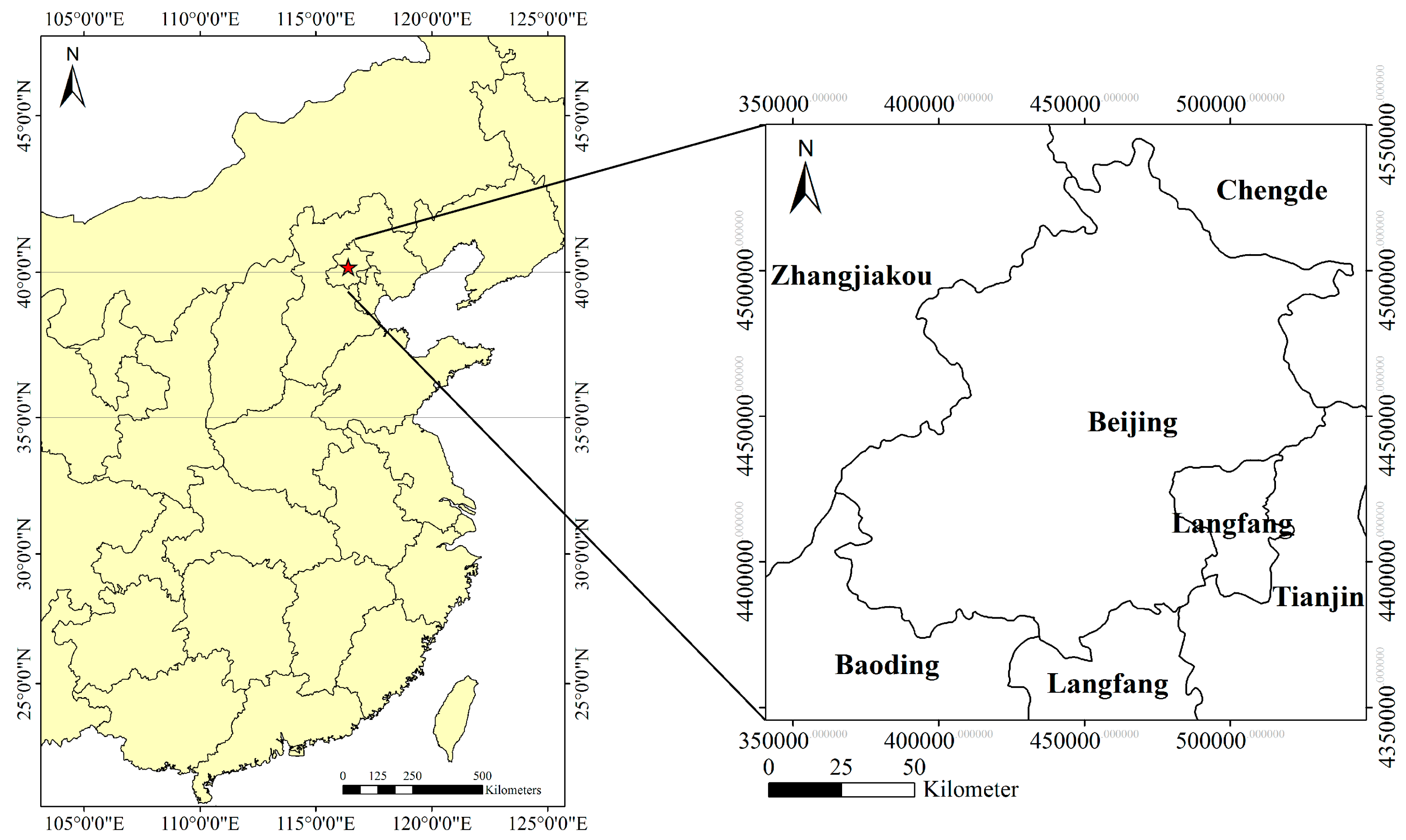
Beijing is located in the northern edge of the North China Plain, covering 16,808 km² between 39°26ʹN and 41°03ʹN latitude and 115°25ʹE and 117°30ʹE longitude (Figure 1). As the capital city of China, Beijing has experienced rapid urban development since the implementation of the reform and opening-up policy in 1978, and agricultural land has declined sharply since then. According to the Second National Land Survey, farmland of Beijing was 22.71 million hectares at the end of 2009, 11.67 million hectares less than it was in 1996. The encroachment of urban land has been a major cause [25]. In order to achieve sustainable development of ecological environment, it is extremely important to continuously monitor farmland change for land use planners.

Figure 1. Study area location.

Figure 1. Study area location.

2.2. MODIS Time Series Data

The MODIS 16-day composite 250 m products (MOD13Q1) for the period January 2001 to December 2010 (23 scenes per year) are downloaded from the Level 1 and Atmosphere Archive and Distribution System (LAADS) website. This product includes four spectral reflectance bands designed for the study of vegetation and land surface, i.e., band 1 (red: 620–670 nm), band 2 (NIR: 841–875 nm), band 3 (blue: 459–479 nm), and band 7 (MIR: 2105–2155 nm). Two tiles (H26V04, H26V05) are mosaicked to cover the study area. The advantages of using MODIS data include their large-scale coverage, high temporal resolution, and open data policy [26].

2.3. Ancillary Data

ESA Global Land Cover (GlobCover) map version 2.3 for 2009 [27] is used as ancillary data for model training. GlobCover 2009 map was produced at 300 m spatial resolution by automatic classification of time series of Medium Resolution Imaging Spectrometer Instrument (MERIS) Fine Resolution surface reflectance mosaics. Based on the GlobCover nomenclature, farmland is marked as class value 11 and 14, while built-up is marked as class value 190. The map is resampled to 250 m resolution to be consistent with MODIS.

Two additional ancillary datasets are used for accuracy assessment. The first dataset are two scenes of Landsat TM (row 32/ path 123) acquired in 31 August 2001 and 8 August 2010, respectively. They are used for the manual selection of a validation set. The other dataset are high spatial resolution images from Google Earth, used for examining the validation set.

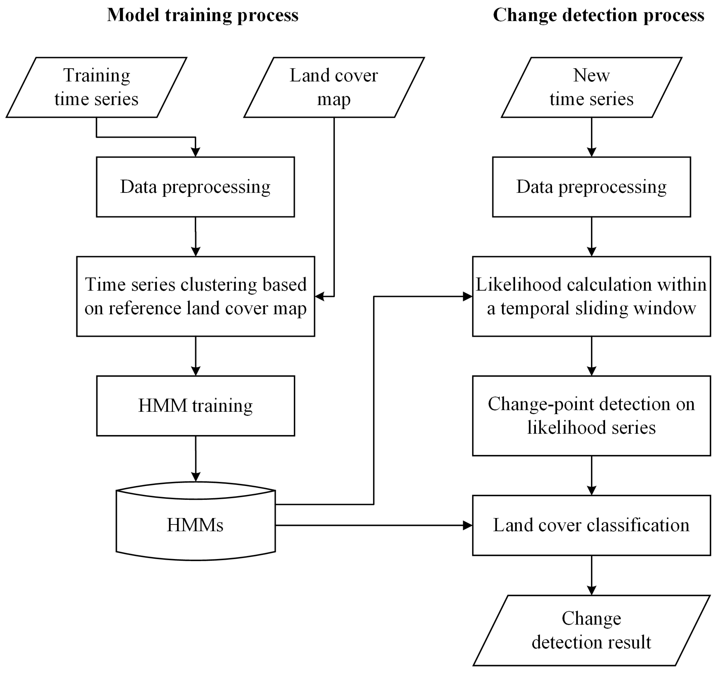
3. Methodology

HCCDC consists of a model training process and a change detection process, as illustrated in Figure 2.

Figure 2. Workflow of the HMM-based continuous change detection and classification (HCCDC) method.

Figure 2. Workflow of the HMM-based continuous change detection and classification (HCCDC) method.

The model training aims at learning an HMM for each land cover class. It includes three major steps: data preprocessing, time series clustering based on reference land cover map, and HMM training. The training data are MODIS time series in 2009, which are consistent with the land cover map of GlobCover 2009 map. The output data are a group of HMMs.

When new time series have been preprocessed, the change detection process finds land cover change by running the following three steps iteratively: likelihood calculation within a temporal sliding window, change detection on likelihood series, and land cover classification. The results include the location, time, and type of a land cover change.

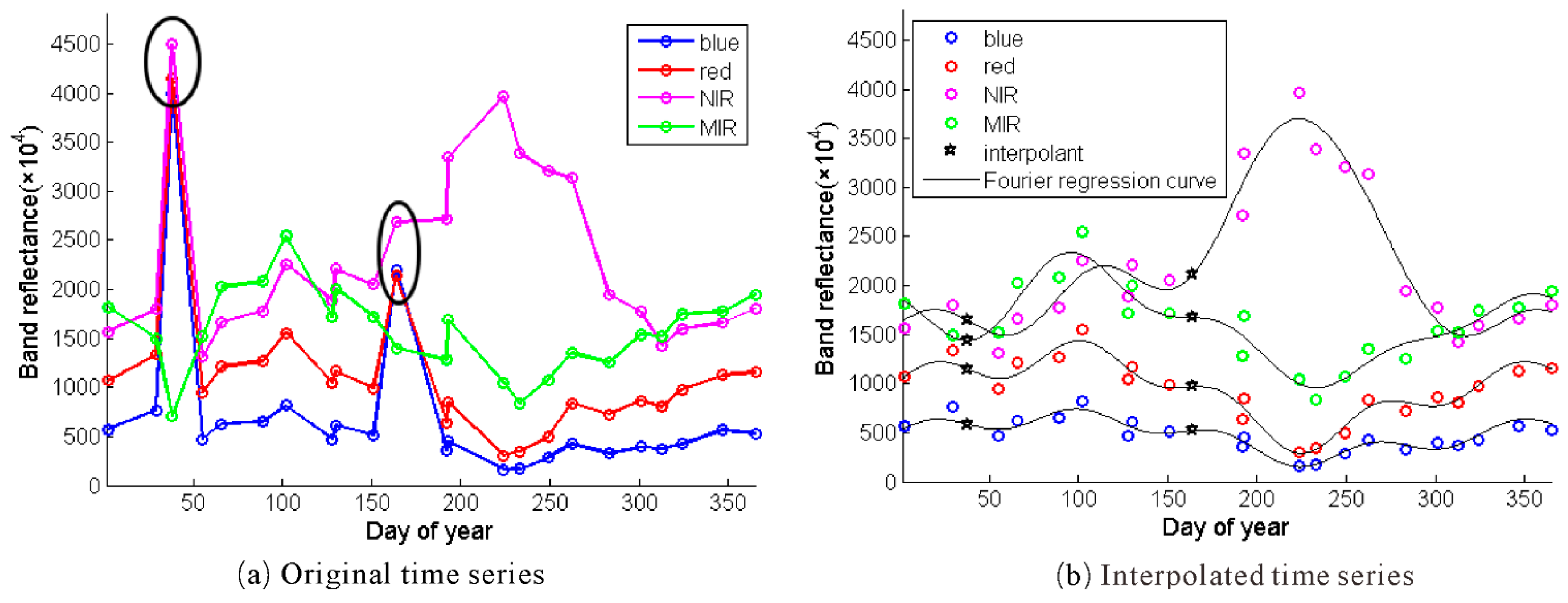
3.1. Data Preprocessing

All MODIS images are projected to UTM 50N zone with WGS84 coordinate system.

Outliers caused by cloud and snow cover are common in satellite image time series. To avoid the impact of outliers on change detection results, it is necessary to reconstruct cloud/snow free time series. The quality flags in the MODIS product are used to identify pixels contaminated by cloud and snow. Some unlabeled cloudy points are also masked if their blue reflectance values are over 0.2, as suggested in [28]. The masked values are then replaced by interpolants obtained by Fourier regression fitting to yearly time series. Fourier regression has been claimed to have several advantages for fitting functional curves to time series of general spectral bands [29]. This procedure is illustrated in Figure 3, where the black circles of Figure 3a indicate the identified noisy points, while the black pentagrams of Figure 3b designate the interpolants.

Figure 3. Fourier regression fitting implemented on time series of a pixel: (a) original time series; and (b) interpolated time series with Fourier regression using only high quality points.

Figure 3. Fourier regression fitting implemented on time series of a pixel: (a) original time series; and (b) interpolated time series with Fourier regression using only high quality points.

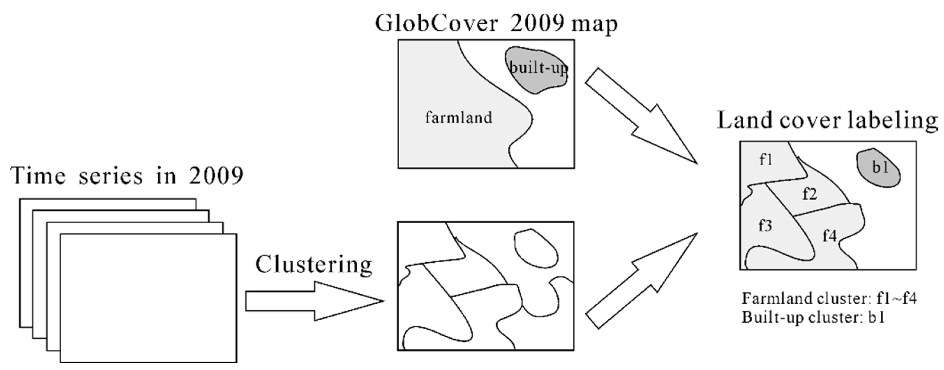
3.2. Time Series Clustering Based on Reference Land Cover Map

A land cover class may include several subclasses with distinct phenological patterns and spectral characteristics. To identify temporal homogeneous land cover classes, the training time series are initially clustered into some clusters using K-Means algorithm, then labeled with the reference land cover map, as shown in Figure 4. The Euclidean distance is used as the similarity measure in the K-Means algorithm. Specifically, for each cluster, its distribution (histogram) is computed in terms of classes of the reference land cover map. If the proportion of a class in the histogram exceeds a certain threshold, the cluster is assigned to this class. According to [30], the clusters obtained by the K-Means algorithm are closely related to the actual vegetation in the local region.

Figure 4. The training time series clustered based on the reference land cover map.

Figure 4. The training time series clustered based on the reference land cover map.

It should be noted that a seemingly more preferable approach would be to cluster time series class by class according to the reference map. In this way, the clusters will directly have a label. However, initial experiments based on this method did not produce good results. This is mainly due to the spatial consistency between MODIS images and GlobCover 2009 map is not satisfied.

3.3. HMM Training

3.3.1. Basic Principles of HMM

In this work, an HMM is used to incorporate the temporal dynamics of each cluster. We adopted HMM because its state-oriented topology represents well the vegetation development in terms of underlying phenological phases with different governing rules [31].

HMM is defined by a compact notation $\mathsf{\lambda }=\langle \pi ,A,B\rangle$ to indicate the complete parameter set, where π, A, B are the initial state distribution vector, the state transition probability distributions, and the observation probability distributions, respectively [32].

$$\pi =\left\{{\pi }_i\right\},{\pi }_i=\text{P}\left(s_1=S_i\right),$$

(1)

$$A=\left\{a_{ij}\right\},a_{ij}=\text{P}\left(s_{t+1}=S_j|s_t=S_i\right),$$

(2)

$$B=\left\{b_i\left(o_t\right)\right\},b_i\left(o_t\right)=\text{P}\left(o_t|s_t=S_i\right),1\le i,j\le N,\text{\hspace{0.17em}}1\le t\le T.$$

(3)

Here, the state set is donated by S= {s_i}; o_t is the observation at time t and s_t is the associated state. T is the total length of the training time series.

In this study, the observations are the multispectral band values, $o_t\in R^4$; and the states implicitly correspond to the phenological phases of local vegetation, as suggested in [33,34,35].

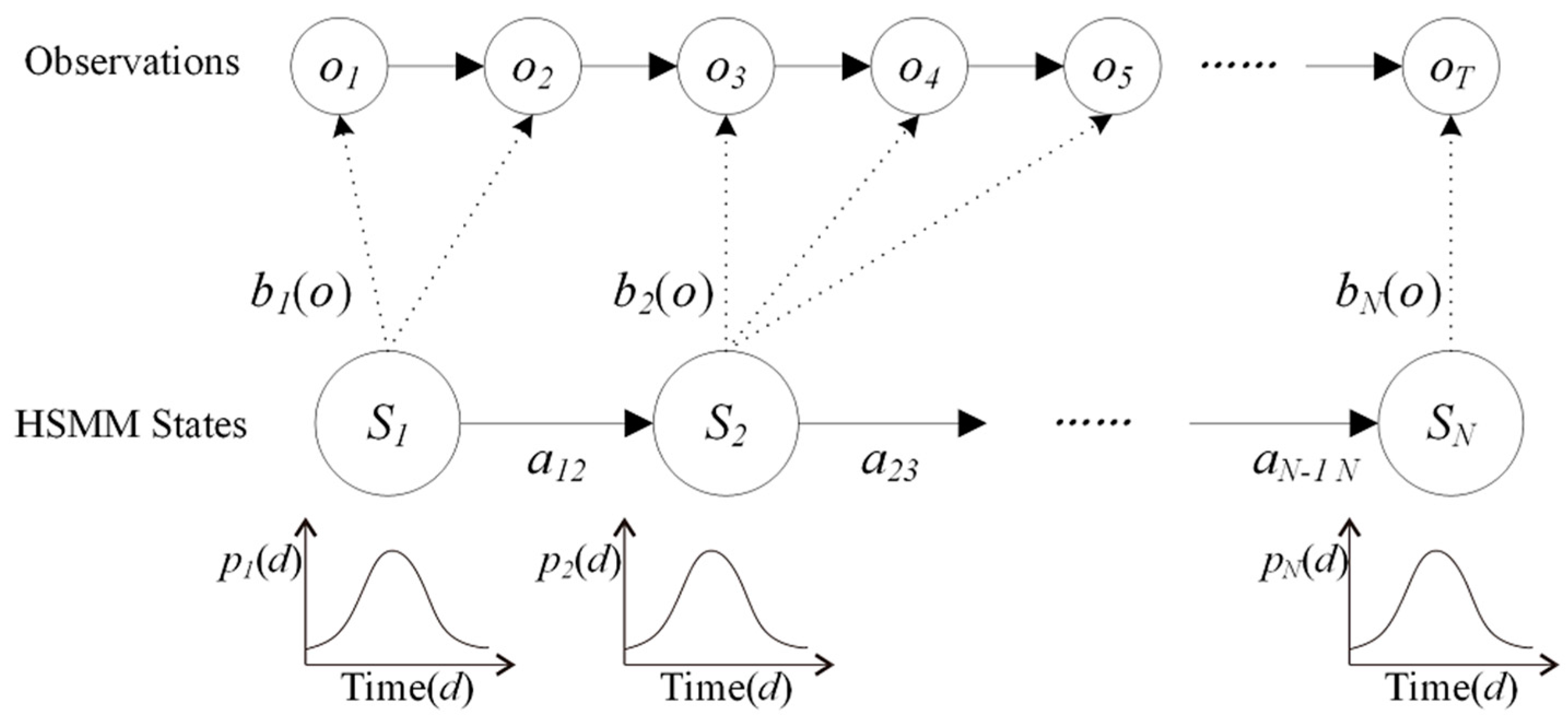
3.3.2. The Extension to Hidden Semi-Markov Model

HMM has an intrinsic limitation. The Markovian hypothesis imposes restrictions on the distribution of the sojourn time in a state, which should be geometric distributed [36]. The geometric distribution is apparently inconsistent with prior knowledge of phenology. For example, the whole growth season of wheat can be divided into five stages: wintering, greening, jointing, heading, and grain filling. The durations of these stages range from 15 to 90 days in length and are non-geometric in terms of distribution. Therefore, HMM does not provide adequate representation of temporal dynamics of a land cover class.

To overcome the limitation of HMM, we relax the Markov assumption by using a hidden semi-Markov model (HSMM) instead [37]. HSMM is a generalized version of HMM, in which one state could produce a sequence of observations with explicit duration. The state duration probability distributions of an HSMM are denoted by D:

$$D=\left\{p_i\left(d\right)\right\},p_i\left(d\right)=\mathrm{P}\left({\tau }_t=d|s_t=S_i\right)$$

(4)

where ${\tau }_t$ denotes the residual time of the current state s_t before time t. Figure 5 provides an example of an HSMM. First, a sample d₁ (i.e., d₁ = 2) is drawn from the state duration distribution p₁ (d) of the first state. Consequently, d₁ observations o₁,…,$o_{d_1}$ are emitted according to the corresponding observation distribution b₁(o). Then the second state is entered and the same process is repeated for the remaining sequence.

Figure 5. Example of a hidden semi-Markov model (HSMM).

Figure 5. Example of a hidden semi-Markov model (HSMM).

3.3.3. Model Specification and Parameter Estimation

Before model training, the structure of the HSMMs should be fitted to the problem. In particular, the number of states, the possible transitions, the types of observation probability distributions B, and the duration probability distributions D have to be determined.

For all clusters, a left–right model topology, with no skip path, has been adopted, this to accommodate for the intra-annual variations. In this model, from each state only the succeeding state is reachable, and the final state cannot convert to any other states. The number of states has been fixed for all the models. The observation probability distributions, B, are modeled as single Gaussian functions, and the duration probability distributions, D, are modeled as Gamma functions. Their parameters have been set empirically.

Given the model structure and a training set O = {O_i, 1 ≤ i ≤ L where L is the number of training samples, some well-established approaches have been proposed to automatically optimize the model parameters by maximizing the observation likelihood P (O|λ). First, individual observations in the time series are clustered using the K-Means algorithm, in order to find the initial parameters of B. Then, an extended Baum–Welch algorithm is employed to train the model, which is claimed to be general to various applications and kinds of data [37].

3.4. Likelihood Calculation within a Temporal Sliding Window

Given the cluster label of a particular pixel at the initial time (obtained by HSMM-based classification), the corresponding model likelihood is calculated over subsequences that are extracted with a temporal sliding window.

A subsequence, with length w and position t, is defined as $o_t\left(w\right)=o_t,o_{t+1},...,o_{t+w-1}$. The sequential subsequences $o_{t_p}\left(w\right),o_{t_p+1}\left(w\right),...$ are extracted using a sliding window, which moves with one time step increment. Here, w is set to 23, which is equal to the number of observations per year. The likelihood calculation is performed on each subsequence, its result being assigned to the last observation (time of the window). In our implementation, the forward-backward algorithm is used to calculate the model likelihood [37].

Figure 6b shows the obtained likelihood series of a pixel. Assume this pixel belongs to the ith cluster in 2001. First a subsequence O₁ (23).is extracted from the time series. The model likelihood P (O₁ (23)|λ_i) of cluster i is calculated and assigned to time t = 23. Then the sliding window moves to the next time step to extract the subsequence O₂ (23), and the same procedure is repeated. Finally, a series of likelihoods is obtained by moving the sliding window through the whole time series.

Figure 6. (a) Likelihood calculation operated on a subsequence within a temporal sliding window. The window is indicated by a grey box. (b) The obtained (log-) likelihood series.

Figure 6. (a) Likelihood calculation operated on a subsequence within a temporal sliding window. The window is indicated by a grey box. (b) The obtained (log-) likelihood series.

It should be noticed that only subsequences starting from the first observation of a year can be directly operated by the algorithm. Since the established model is noncyclic, it is unable to calculate the transition probability from the last observation of a year to the first observation of the next year. To cope with this problem, we rearrange individual observations in a sub-sequence according to their sequential number in a year. For example, the mth observation in the nth year is donated as $o_m^n$. A subsequence $o_m^n,o_{m+1}^n,...o_{23}^n,o_1^{n+1},...,o_{m-1}^{n+1},\text{\hspace{0.17em}\hspace{0.17em}}m\ne 1$ is converted to $o_1^{n+1},o_2^{n+1}...,o_{m-1}^{n+1},o_m^n,...,o_{22}^n,o_{23}^n$ after the rearrangement. The proof of the validity of this rearrangement is given in the supplement of this paper. Moreover, we illustrate in Section 5.3 that the HSMM accommodates to the data rearrangement when the class of the observation sequence does change from one year to another.

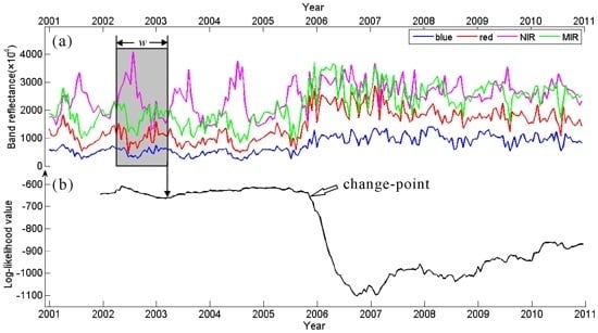
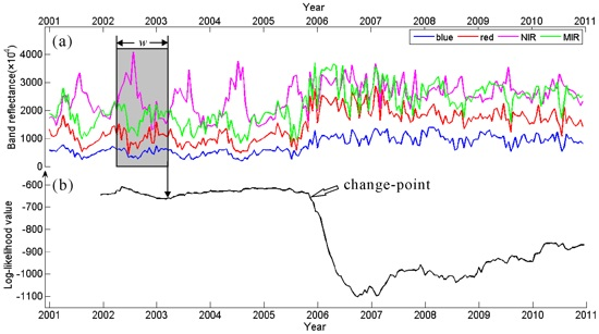
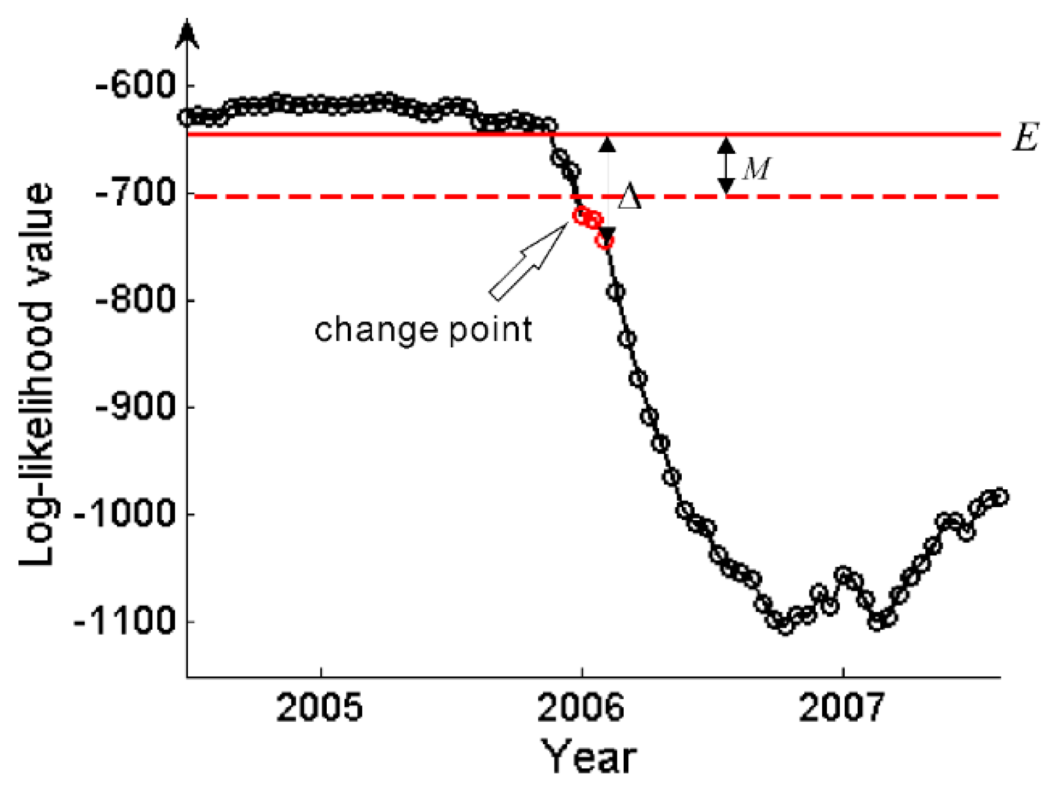
3.5. Change Detection on Likelihood Series

The major contribution of this paper is a novel procedure to detect land cover change based on likelihood change. Indeed, as it can be seen in Figure 6, when there is no change before 2005, the likelihoods are relatively high. When a change occurs at the end of 2005, the likelihoods decline sharply and stay low in the subsequent time period. In our approach this is implemented as follows, if the likelihood is lower than a threshold, M, for three consecutive times, a change is detected. Formally, this is achieved as follows.

The mean likelihood of each cluster is estimated on the training time series O = {O_i}, 1 ≤ I ≤ L:

$$E=\frac{1}{L}{\displaystyle \sum _{i=1}^L\log \text{P}\left(O_i|\mathsf{\lambda }\right)}$$

(5)

The difference between the likelihood of subsequence o_t (w) and E is:

$$\Delta =E-\log \text{P}\left(o_t\left(w\right)|\mathsf{\lambda }\right)$$

(6)

If $\Delta$ is larger than a threshold M for three consecutive times, a change is identified. Otherwise, if $\Delta$ for only one or two consecutive observations is larger than M, it is regarded as a temporary change. When a change is detected, the first observation for which $\Delta$ is larger than M is identified as an approximate change-point. Since M may be different for distinct clusters, it is set to γ times of the standard deviation (STD) of the likelihoods for each cluster:

$$M=\gamma \cdot \sqrt{\frac{1}{L}{\displaystyle \sum _{i=1}^L{\left(\text{P}\left(O_i|\mathsf{\lambda }\right)-E\right)}^2}}$$

(7)

Figure 7 illustrates the proposed change detection procedure on likelihood series. By running this procedure continuously on incoming time series, changes can be detected in near real-time.

Figure 7. Change detection operated on a likelihood series. The red solid line shows the mean likelihood, and the red dashed line marks the minimum value for unchanged likelihood. The likelihoods highlighted in red are considered as changed. The arrow indicates the approximate change-point.

Figure 7. Change detection operated on a likelihood series. The red solid line shows the mean likelihood, and the red dashed line marks the minimum value for unchanged likelihood. The likelihoods highlighted in red are considered as changed. The arrow indicates the approximate change-point.

3.6. Land Cover Classification

Once a change is detected, it is necessary to know the land cover class after the change. Instead of classifying individual images using conventional methods, the trained HSMMs are used for land cover classification as a standard Bayesian maximum posteriori probability (MAP) classifier: A pixel is classified into the cluster whose corresponding model achieves the maximum likelihood among all the models on the yearly time series after the change-point. If the cluster labels of a pixel before and after the change belong to different classes, a real land cover change is detected. Otherwise, if the cluster labels before and after the change belong to the same land cover class, the identified change is considered as a false alarm. HMM-based classification procedure has been reported in previous studies and has achieved good performance [34,35]. In this study, HSMM and HMM give comparable classification performance.

After land cover classification, the change detection process is restarted on incoming time series to monitor land cover change continuously.

4. Validation

4.1. Feasibility Analysis

In this study, we apply HCCDC to monitor urban encroachment upon agricultural land in Beijing. Two land cover classes are considered in the case study: farmland and built-up. The basic hypothesis underlying this study is that when the sensed area of a pixel converts from farmland to built-up, the model likelihoods of farmland will drop sharply. Hence, it is required that the established models have good separability between farmland and built-up. This assumption will be verified through experiments over the training data.

4.2. Validation Dataset

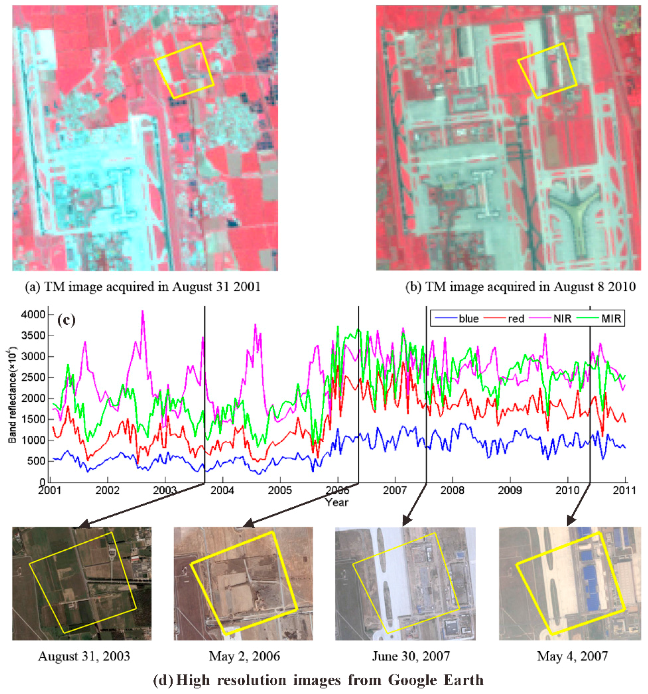
Since it is difficult to find reliable ground truth to evaluate the change detection performance, a manually selected validation set from Landsat TM images is used for accuracy assessment, as proposed in [6]. The validation set is composed of a total of 500 pixels, in which 250 pixels are from farmland areas where the land cover class are persistent throughout the time of analysis, and 250 pixels are selected within the areas where conversions from farmland to built-up are found. The validation samples are examined using high resolution images from Google Earth before and after a possible change. The ENVI region of interest (ROI) tool is used to export digitized ROIs to a vector file, which is imported into Google Earth to examine whether interested changes occur. 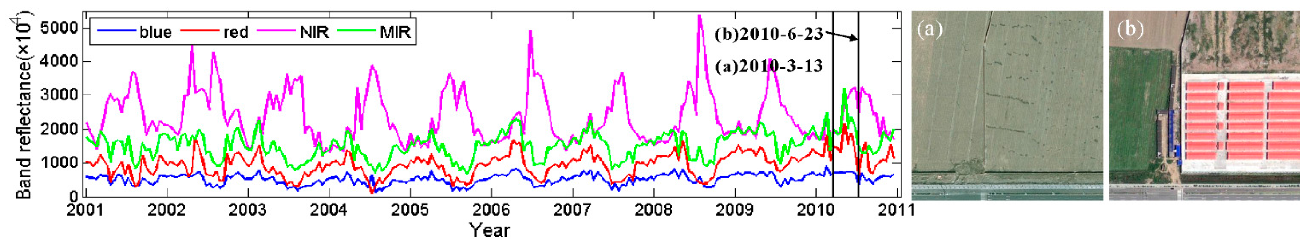Figure 8c shows a changed pixel in the validation set. Its corresponding area is manually digitalized from the Landsat TM images (Figure 8a,b) and overlaid with high resolution images from Google Earth (Figure 8d).

Figure 8. A changed pixel in the validation set. The reference Landsat TM images acquired in (a) 2001 and (b) 2010, respectively, where the changed area is marked with a yellow polygon; (c) time series of the corresponding pixel in the MODIS images; and (d) high resolution images from Google Earth.

Figure 8. A changed pixel in the validation set. The reference Landsat TM images acquired in (a) 2001 and (b) 2010, respectively, where the changed area is marked with a yellow polygon; (c) time series of the corresponding pixel in the MODIS images; and (d) high resolution images from Google Earth.

4.3. Comparison with Other Approaches

The performance of HCCDC is compared with the outcomes of other change detection approaches. One is the CCDC algorithm proposed in [6]. It is based on pixel-wise curve fitting. If the differences between observed and predicted pixel values are larger than a threshold for three consecutive times, a change is identified. Then the model parameters are re-estimated on incoming time series after change and used for land cover classification. HCCDC is also compared with a post-classification change detection (PCCD) method developed in [38]. PCCD detects change by implementing a temporal moving window over a series of land cover maps. Two consecutive years of farmland or built-up is assumed.

All these algorithms are able to detect multiple changes, but only the last change is used for accuracy assessment. It is because the change from farmland to built-up is generally irreversible. Built-up areas usually do not change any more.

5. Results and Discussion

5.1. Results of Time Series Clustering

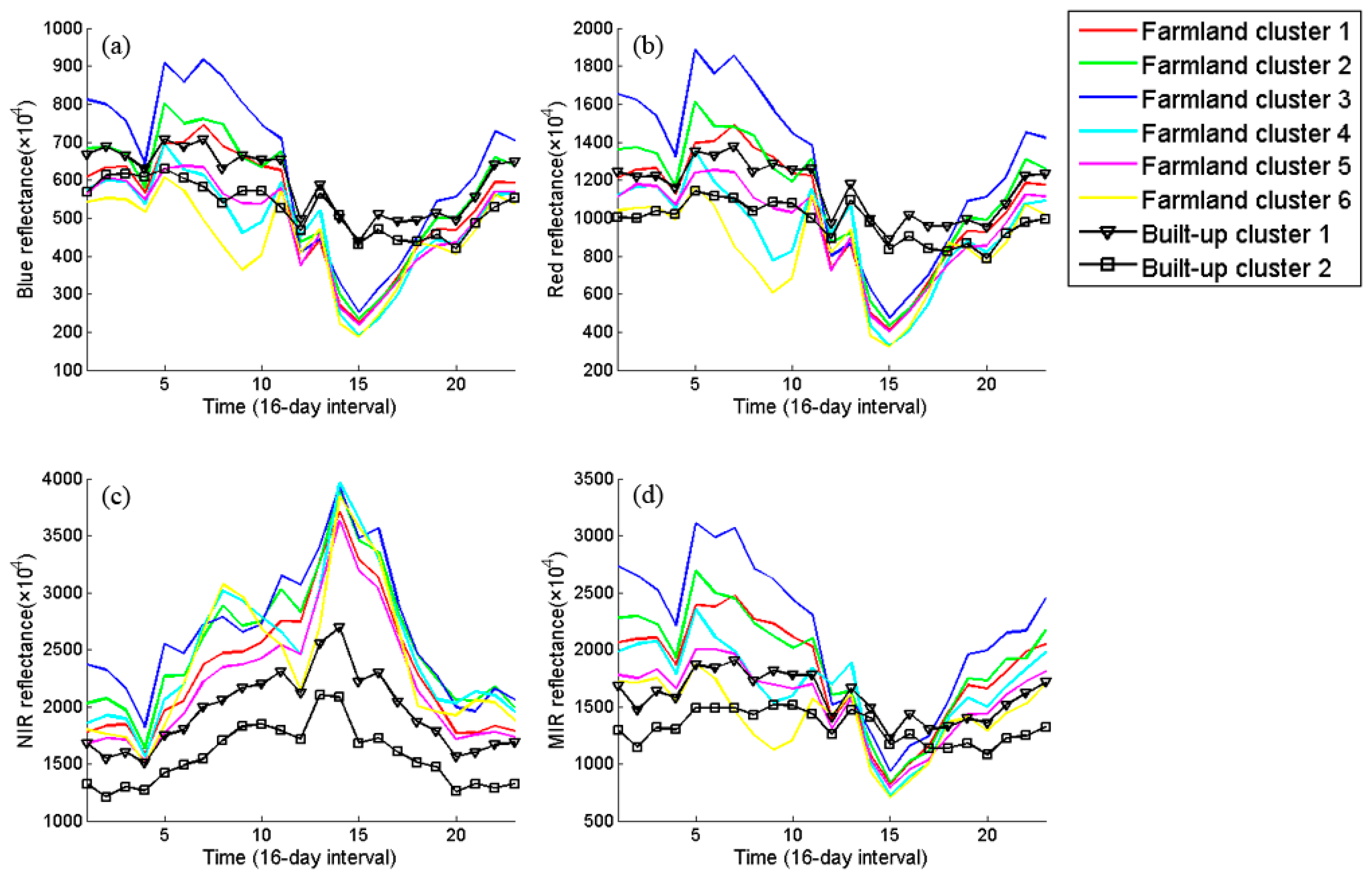
The time series in 2009 are automatically clustered into 30 clusters. According to GlobCover 2009 map, six of them are labeled as farmland while two are assigned to built-up. Figure 9 illustrates the cluster centroid for each spectral band. We can see that for farmland clusters, seasonal variations in all the spectral bands are significant. Specifically, the NIR reflectance profiles of cluster 4 and 6 have two peaks a year while the others have only one, due to different cropping systems (monocropped vs. double-cropped). In contrast, variations in built-up clusters are relatively weak. In particular, the NIR reflectance values of cluster 1 are higher than those of cluster 2, due to the vegetation cover, such as trees and lawns within the urban areas.

Figure 9. Time series of K-Means centroids. Surface reflectance bands: (a) blue, (b) red, (c) NIR, and (d) MIR.

Figure 9. Time series of K-Means centroids. Surface reflectance bands: (a) blue, (b) red, (c) NIR, and (d) MIR.

5.2. Results of the Feasibility Analysis

Five-state HSMMs are taken as an example for this feasibility analysis. The histogram of log-likelihoods of each built-up cluster produced by the model of each farmland cluster is illustrated in red in Figure 10. The histogram of the farmland cluster itself is shown in blue. It can be seen that there is significant difference in likelihood distribution between built-up and farmland: the likelihoods for most farmland samples are within the range (−650, −550) but for built-up samples, they are less than −600. Therefore, we can use the model likelihood of HSMM to distinguish built-up from farmland.

Figure 10. (a) The log-likelihood distribution of built-up cluster 1 produced by the model of each farmland cluster. (b) The log-likelihood distribution of built-up cluster 2 produced by the model of each farmland cluster.

Figure 10. (a) The log-likelihood distribution of built-up cluster 1 produced by the model of each farmland cluster. (b) The log-likelihood distribution of built-up cluster 2 produced by the model of each farmland cluster.

5.3. Likelihood Series of Rearranged Observation Sequences

In this section, we illustrate that HSMM accommodates to the observation rearrangement, when the class of the observed sequence does change from one year to another. Figure 11 illustrates the three-year time series of a pixel, which converts from farmland to built-up land use. The change occurs at time t = 44 (marked with a black line).

Figure 11. The three-year time series of a pixel with class change.

Figure 11. The three-year time series of a pixel with class change.

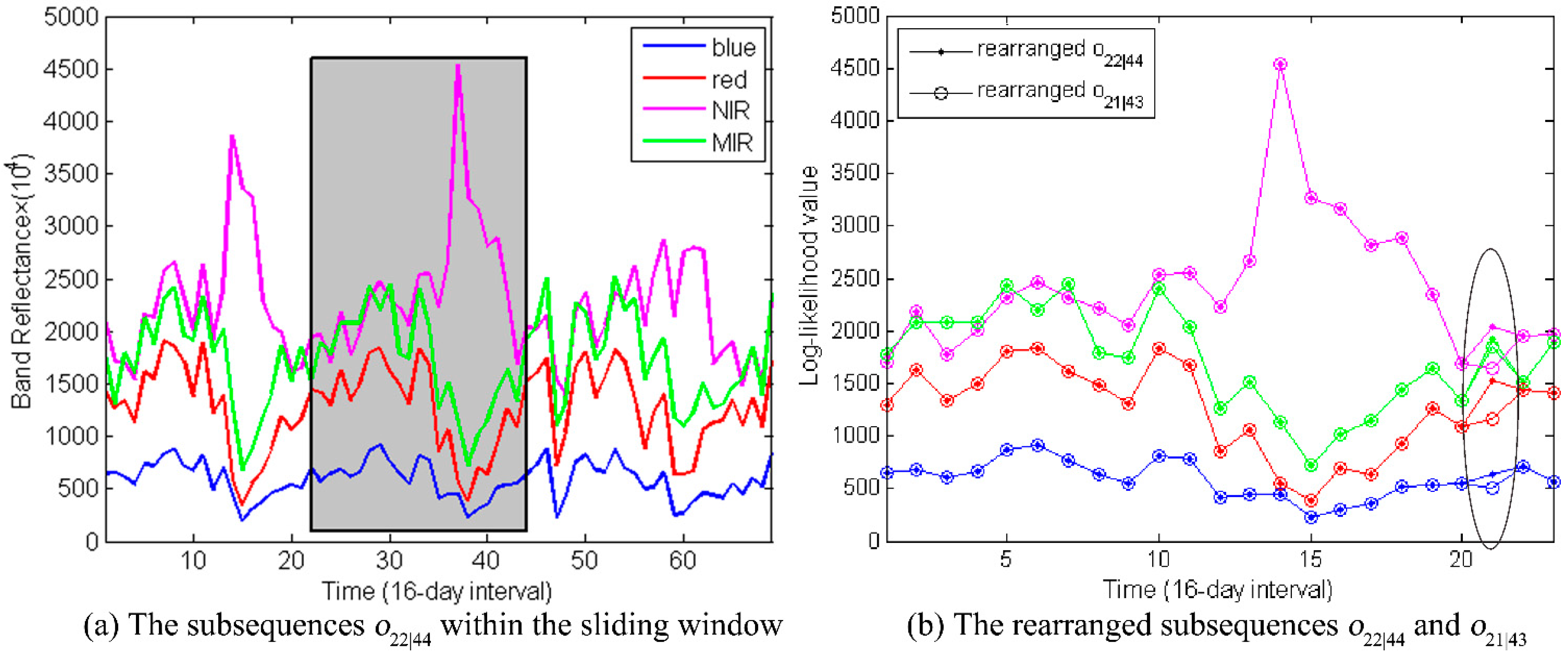
The first changed subsequence $o_{22|44}$ after the arrangement is shown in Figure 12. Compared to its previous subsequence $o_{21|43}$, though only one observation is different ($o_{44}$ vs. $o_{21}$), the log-likelihood declined from –640 to –644.

Figure 12. (a) The subsequences $o_{22|44}$ is indicated within the grey window. (b) The rearranged subsequence $o_{22|44}$ and $o_{21|43}$ are displayed. Only one observation between them is different, which is highlighted within the black circle. The other observations are overlapping displayed.

Figure 12. (a) The subsequences $o_{22|44}$ is indicated within the grey window. (b) The rearranged subsequence $o_{22|44}$ and $o_{21|43}$ are displayed. Only one observation between them is different, which is highlighted within the black circle. The other observations are overlapping displayed.

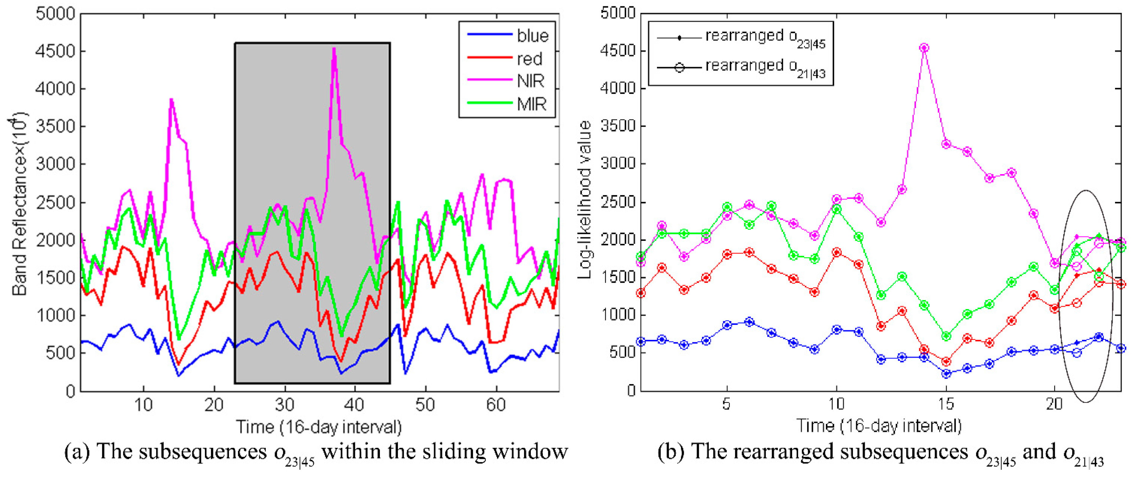
Then we move the sliding window a time step further. The obtained subsequence $o_{23|45}$ is shown in Figure 13. Its log-likelihood is −643.

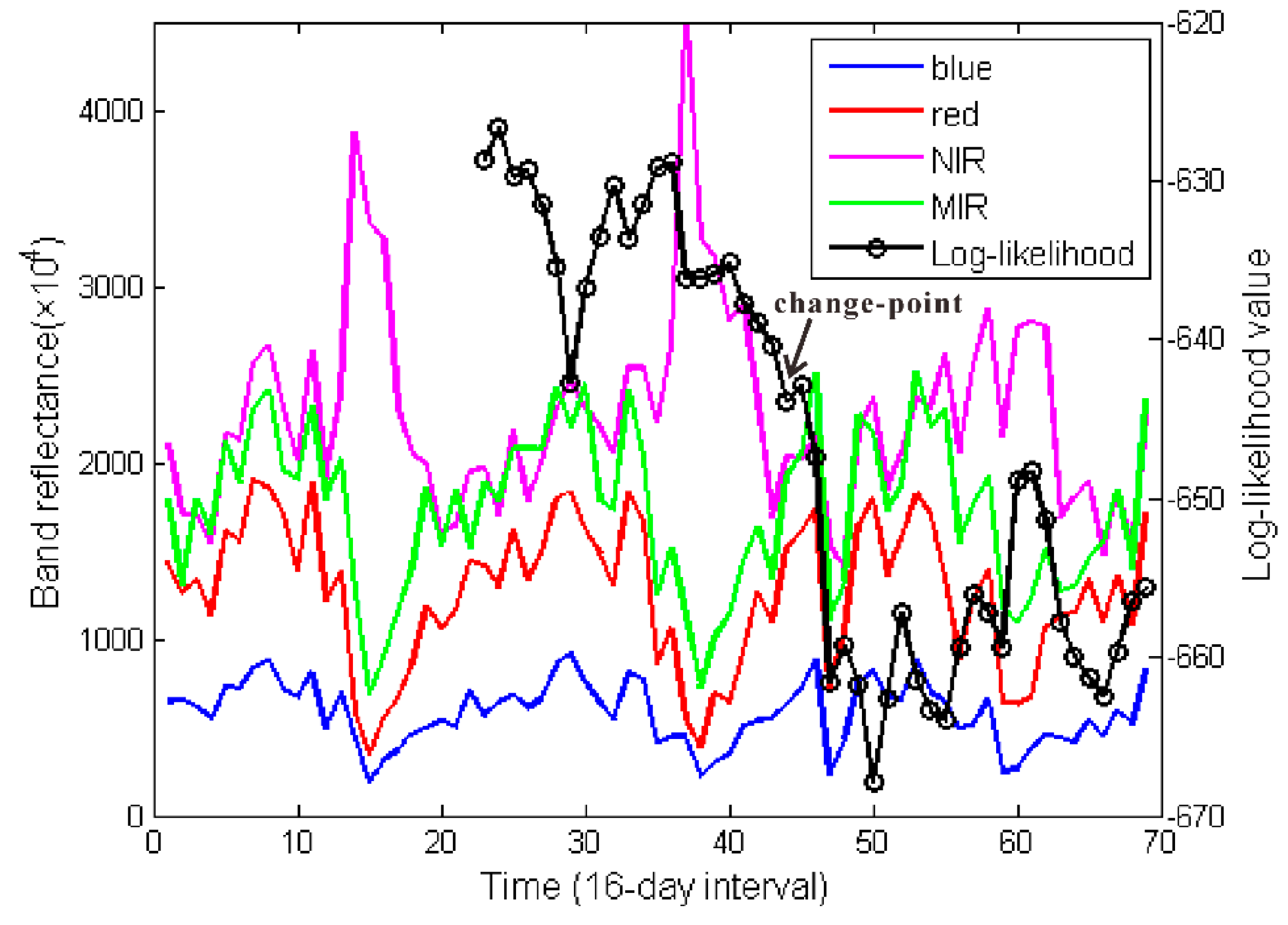
Repeating the above process for the whole time series, we obtain the likelihood series where the detected change corresponds to the class change (Figure 14). This example demonstrates that, when there is a class change, the rearranged subsequence will drop because it no longer fits the trained HSMM.

Figure 13. (a) The subsequences $o_{23|45}$ is indicated within the sliding window. (b) The rearranged subsequence $o_{23|45}$ and $o_{21|43}$ are displayed. Two observations between them are different, which are highlighted within the black circle. The other observations are overlapping displayed.

Figure 13. (a) The subsequences $o_{23|45}$ is indicated within the sliding window. (b) The rearranged subsequence $o_{23|45}$ and $o_{21|43}$ are displayed. Two observations between them are different, which are highlighted within the black circle. The other observations are overlapping displayed.

Figure 14. The original time series and the obtained likelihood series are displayed together. The arrow indicates the detected change-point.

Figure 14. The original time series and the obtained likelihood series are displayed together. The arrow indicates the detected change-point.

5.4. Accuracy Assessment

Both HCCDC and CCDC are pre-classification algorithms. In this section, we evaluate their performance for the change detection step and the classification step separately. Then the final change detection accuracy is compared with that of PCCD.

5.4.1. Accuracy Assessment for Change Detection

We train HSMMs with different number of states ranging from three to eight, to find the optimal one. The receiver operating characteristic (ROC) analysis is used to evaluate the change detection performance, without committing to a single decision threshold [39]. For both HCCDC and CCDC, the thresholds are varied to generate an ROC curve (Figure 15). Corresponding equal error rates (EER) and the area under the curve (AUC) are obtained. Table 1 shows the change detection accuracy of HCCDC with different number of states. By referring to Figure 15, the ROC curves of all the algorithms are similar. The best result is achieved by four-state HSMM, with EER of 20.00% and AUC of 0.882. It also shows that three or four states are sufficient to identify changes from farmland time series. In comparison, the obtained EER and AUC by CCDC are 20.32% and 0.869, respectively. Such results indicate that HCCDC can achieve comparable change detection accuracy with CCDC.

Figure 15. The receiver operating characteristic (ROC) curves of true positive rates (TPRs) versus false positive rates (FPRs). Each point represents a pair of TPR and FPR obtained under different thresholds.

Figure 15. The receiver operating characteristic (ROC) curves of true positive rates (TPRs) versus false positive rates (FPRs). Each point represents a pair of TPR and FPR obtained under different thresholds.

Table 1. Change detection accuracy for HCCDC with different number of states.

Number of States	EER	AUC
3	20.16%	0.879
4	20.00%	0.882
5	22.63%	0.869
6	23.20%	0.864
7	23.75%	0.848
8	22.15%	0.856

Note: EER, equal error rates; AUC, area under the curve.

Table 1. Change detection accuracy for HCCDC with different number of states.

Number of States	EER	AUC
3	20.16%	0.879
4	20.00%	0.882
5	22.63%	0.869
6	23.20%	0.864
7	23.75%	0.848
8	22.15%	0.856

Note: EER, equal error rates; AUC, area under the curve.

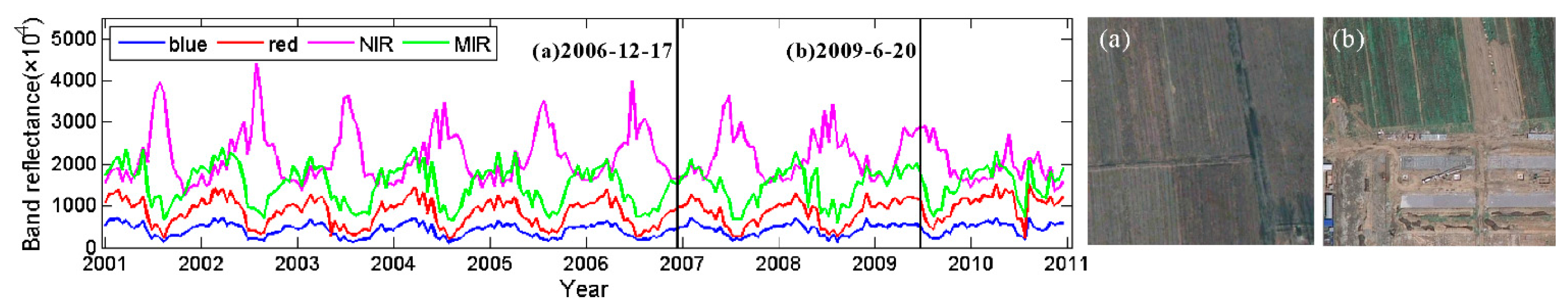
The omission errors of HCCDC result from the following reasons: (1) partially changed pixels; (2) high coverage of urban vegetation; and (3) changes occur too late during the time of analysis. Due to the low spatial resolution of MODIS images, change in a part of a pixel is hard to detect. In Figure 16, though half of the (pixel) area has been converted into a construction site, change in the time series is minor. In addition, when built-up regions are covered with high density plants, they are easily to be confused with farmland. Finally, as we are dealing with changes between 2001 and 2010, if a change happens at the end of 2010, it is hard to find three consecutive observations whose likelihoods are less than the threshold M. In Figure 17, a change occurred in mid-2010. However, there are only eleven observations left for identifying the change.

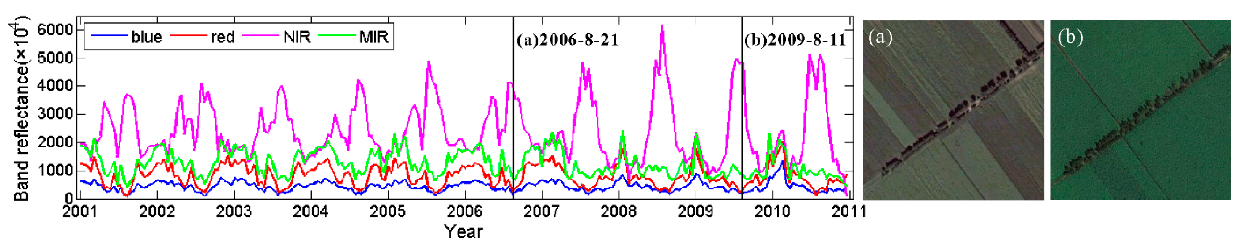
The commission errors (or “false positives”) of HCCDC are mostly due to the following reasons: (1) overfitting of the model; (2) switching of crop types. On one hand, the overfitting problem caused by using too many states makes the model sensitive to noises in time series. On the other hand, some unchanged pixels in the validation set were actually diverted to other types of crop during the time of analysis, causing changes in temporal development curves. For example, in Figure 18, the sensed area of an unchanged pixel was switched from a typical double-cropping system to monocropping round 2007, resulting in a change identified by the algorithm.

Figure 16. Omission error in change detection: partially changed pixel. The black vertical line marks the time of the corresponding Google Earth image displayed on the right. (a) 17 December 2006, (b) 20 June 2009.

Figure 16. Omission error in change detection: partially changed pixel. The black vertical line marks the time of the corresponding Google Earth image displayed on the right. (a) 17 December 2006, (b) 20 June 2009.

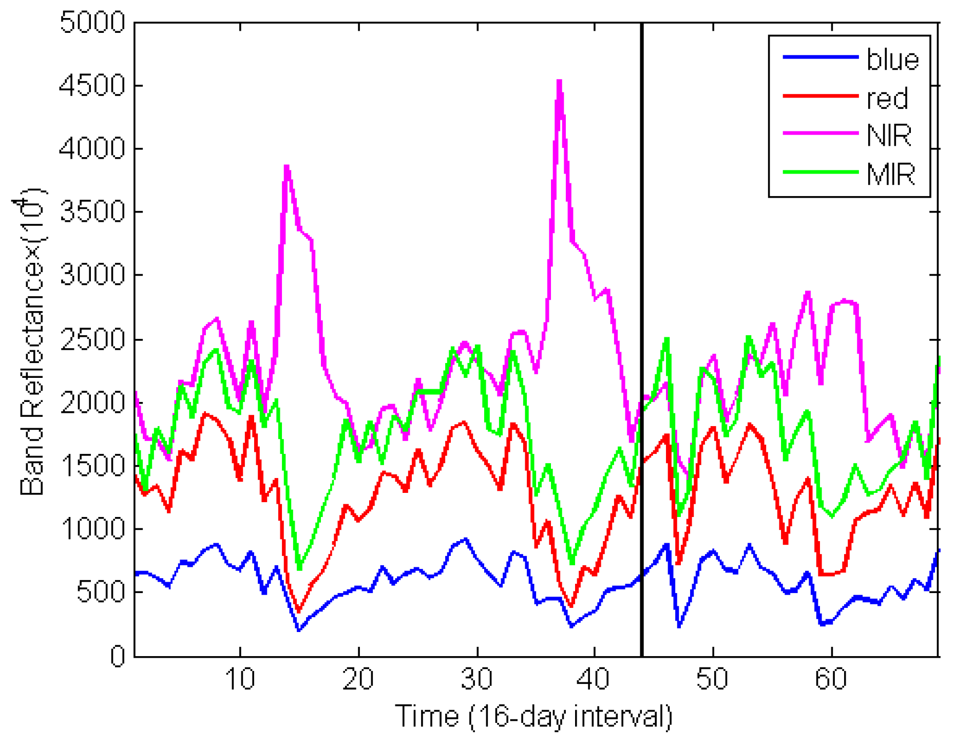
Figure 17. Omission error in change detection: change occurs too late. The black vertical line marks the time of the corresponding Google Earth image displayed on the right. (a) 13 March 2010, (b) 23 June 2010.

Figure 17. Omission error in change detection: change occurs too late. The black vertical line marks the time of the corresponding Google Earth image displayed on the right. (a) 13 March 2010, (b) 23 June 2010.

Figure 18. Commission error in change detection: switching to another crop type. The black vertical line marks the time of the corresponding Google Earth image displayed on the right. (a) 21 August 2006, (b) 11 August 2009.

Figure 18. Commission error in change detection: switching to another crop type. The black vertical line marks the time of the corresponding Google Earth image displayed on the right. (a) 21 August 2006, (b) 11 August 2009.

5.4.2. Accuracy Assessment for Classification

To assess the land cover classification accuracy, we set the threshold γ of HCCDC equal to 1 and classify all the changed pixels identified by the algorithm. The results are listed in Table 2. Here, the producer accuracy (PA) is the fraction of correctly classified pixels with regard to the extracted pixels of that class. The overall accuracy is calculated by summing the number of pixels classified correctly and dividing by the total number of the extracted pixels. According to Table 2, eight-state HSMM achieves the optimal overall (OA) classification accuracy (96.88%). It means that when eight-state HSMMs are used, 235 among 248 changed pixels are correctly detected and classified, at the same time, only one of the unchanged pixels is considered converted into built-up. Moreover, HSMMs using five to eight states perform better than those with three or four states. In all the cases, PA of farmland is better than that of built-up. This may be attributed to more number of clusters used for farmland, resulting in better modeling accuracy. It also indicates that most of the false changes can be eliminated in the land cover classification step.

Table 2. Classification accuracy for HCCDC using different number of states.

Number of States	Number of the Extracted Pixels		Number of Correctly Classified Pixels		PA		OA
	Built-up	Farmland	Built-up	Farmland	Built-up	Farmland
3	242	153	217	152	89.67%	99.35%	93.42%
4	250	163	227	163	90.80%	100.00%	94.43%
5	250	178	237	177	94.80%	99.44%	96.73%
6	249	178	233	175	93.57%	98.31%	95.55%
7	248	196	231	195	93.15%	99.49%	95.95%
8	248	201	235	200	94.76%	99.50%	96.88%

Note: PA, producer’s accuracy; OA, overall accuracy.

Table 2. Classification accuracy for HCCDC using different number of states.

Number of States	Number of the Extracted Pixels		Number of Correctly Classified Pixels		PA		OA
	Built-up	Farmland	Built-up	Farmland	Built-up	Farmland
3	242	153	217	152	89.67%	99.35%	93.42%
4	250	163	227	163	90.80%	100.00%	94.43%
5	250	178	237	177	94.80%	99.44%	96.73%
6	249	178	233	175	93.57%	98.31%	95.55%
7	248	196	231	195	93.15%	99.49%	95.95%
8	248	201	235	200	94.76%	99.50%	96.88%

Note: PA, producer’s accuracy; OA, overall accuracy.

According to the ROC analysis, two times the root mean square error (RMSE) is used for thresholding for CCDC. The corresponding OA is 81.63%, where 171 among 247 changed pixels are correctly detected and classified (PA of built-up is 69.23%), at the same time, 189 among 194 unchanged pixels are detected and recognized as false alarms (PA of farmland is 97.42%). The results demonstrate that HCCDC performs better in determining land cover class compared to CCDC.

Taking consideration of both change detection and classification steps, the comprehensive accuracy can also be derived. Using five states and setting $\gamma$ to 1, the change detection rate of HCCDC is 94.80% with the false alarm rate of 0.40%. In comparison, the change detection rate of CCDC is only 68.40% with the false alarm rate of 2.00%, while that of PCCD is 89.6% with the false alarm rate of 0.40%. The comparison results indicate that the proposed method is better than the pixel-oriented change detection methods and the post-classification methods to some extent.

5.4.3. Computational Efficiency

To compare the computation time of HCCDC and CCDC, measurements are performed on a 3.2-GHz quad-core machine with 8-GB main memory. Both algorithms are implemented and tested in Matlab^®. For processing 500 time series, a five-state HCCDC requires 244 seconds compared to 306 seconds required by CCDC. By comparison, HCCDC is more computationally efficient. It may be because HCCDC does not need to retrain a new model when change occurs. The high efficiency of our method can improve the processing on large datasets.

6. Strengths and Limitations of HCCDC

Satellite image time series (SITS) provide striking temporal information regarding earth surface development, which makes them a better data source for land use/land cover studies. The proposed HCCDC method is designed for high temporal frequency time series and can be used for unsupervised change detection and classification.

There are some remarkable advantages of HCCDC. (1) The change detection process is fully automated and is able to monitor land cover change as soon as new observations become available. Compared to post-classification algorithms, such as PCCD, HCCDC is capable of detecting inner-annual changes and avoids the impact of classification errors on change detection. (2) HCCDC can provide detailed “from–to” change information compared to previous pre-classification algorithms. (3) HCCDC is more computationally efficient and storage-saving in comparison with the pixel-oriented methods, such as CCDC. Since HCCDC is land cover class oriented, there is no need to train a specified model for each pixel or update the model when new data are entered. This characteristic makes HCCDC more practical for regional or global land cover monitoring.

HCCDC also has limitations. First of all, training HMM needs a lot of samples. However, if there is no available land cover map, visual interpretation of a large number of training samples is very time-consuming and laborious. Second, HCCDC requires high temporal frequency of clear observations. The existence of too many noisy pixels could lead to inferior modeling results. Therefore, the preprocessing step has a strong impact on the following model training and change detection processes.

7. Conclusions

In this paper, a novel SITS-based algorithm—HCCDC, was proposed for continuous land cover change detection and classification. The idea is to observe the likelihood change of a pre-trained HMM for the initial class of a pixel on incoming time series, and detect changes from the dramatic drop of likelihoods. The HSMMs are then used for land cover classification after change to provide “from–to” information.

To evaluate the performance of the proposed method, a case study has been conducted for monitoring urban encroachment onto farmland in Beijing. The results demonstrated that HCCDC is capable of detecting farmland changes and identifying change types. The optimal result of HCCDC was achieved using five states, with the final change detection rate of 94.80% and the false alarm rate of 0.4%. HCCDC was also compared with the CCDC algorithm. The comparison results suggested that HCCDC can achieve comparable change detection accuracy (e.g., with the best EER of 20.00% and AUC of 0.882 for HCCDC, vs. EER of 20.32% and AUC of 0.869 for CCDC) and better classification performance (e.g., with the best OA of 96.88% for HCCDC, vs. 81.63% for CCDC). In addition, HCCDC is also more computationally efficient (e.g., required 244 seconds, vs. 306 seconds for CCDC).

Though the described example was performed on farmland and built-up, HCCDC is also applicable for the near real-time change detection for a large range of land cover classes.

References

- Coppin, P.; Jonckheere, I.; Nackaerts, K.; Muys, B.; Lambin, E. Digital change detection methods in ecosystem monitoring: A review. Int. J. Remote Sens. 2004, 25, 1565–1596. [Google Scholar] [CrossRef]
- Guedon, Y. Segmentation uncertainty in multiple change-point models. Stat. Comput. 2015, 25, 303–320. [Google Scholar] [CrossRef]
- Tsai, C.Y.; Shieh, Y.C. A change detection method for sequential patterns. Decis. Support. Syst. 2009, 46, 501–511. [Google Scholar] [CrossRef]
- Kleynhans, W.; Salmon, B.P.; Olivier, J.C.; van den Bergh, F.; Wessels, K.J.; Grobler, T.L.; Steenkamp, K.C. Land cover change detection using autocorrelation analysis on MODIS time-series data: Detection of new human settlements in the Gauteng province of South Africa. IEEE J. Sel. Topics Appl. Earth Obs. Remote Sens. 2012, 5, 777–783. [Google Scholar] [CrossRef]
- Jamali, S.; Jönsson, P.; Eklundh, L.; Ardö, J.; Seaquist, J. Detecting changes in vegetation trends using time series segmentation. Remote Sens. Environ. 2015, 156, 182–195. [Google Scholar] [CrossRef]
- Zhu, Z.; Woodcock, C.E. Continuous change detection and classification of land cover using all available Landsat data. Remote Sens. Environ. 2014, 144, 152–171. [Google Scholar] [CrossRef]
- Grobler, T.L.; Ackermann, E.R.; van Zyl, A.J.; Olivier, J.C.; Kleynhans, W.; Salmon, B.P. Using Page’s cumulative sum test on MODIS time series to detect land-cover changes. IEEE Geosci. Remote Sens. Lett. 2013, 10, 332–336. [Google Scholar] [CrossRef]
- Jung, M.; Chang, E. NDVI-based land-cover change detection using harmonic analysis. Int. J. Remote Sens. 2015, 36, 1097–1113. [Google Scholar]
- Salmon, B.P.; Olivier, J.C.; Wessels, K.J.; Kleynhans, W.; van den Bergh, F.; Steenkamp, K.C. Unsupervised land cover change detection: meaningful sequential time series analysis. IEEE J. Sel. Topics Appl. Earth Obs. Remote Sens. 2011, 4, 327–335. [Google Scholar] [CrossRef]
- Cho, S.B.; Park, H.J. Efficient anomaly detection by modeling privilege flows using hidden Markov model. Comput. Secur. 2003, 22, 45–55. [Google Scholar] [CrossRef]
- Zeng, J.; Liu, X.J.; Li, T.; Li, G.Y.; Li, H.B.; Zeng, J.Q. A novel intrusion detection approach learned from the change of antibody concentration in biological immune response. Appl. Intell. 2011, 35, 41–62. [Google Scholar] [CrossRef]
- Andrade, E.L.; Blunsden, S.; Fisher, R.B. Hidden Markov models for optical flow analysis in crowds. In Proceedings of the IEEE International Conference on Pattern Recognition, Hong Kong, China, 20–24 August 2006; pp. 460–463.
- Pruteanu-Malinici, I.; Capin, L. Infinite hidden Markov models and ISA features for unusual-event detection in video. In Proceedings of the IEEE International Conference on Image Processing, San Antnio, TX, USA, 16–19 September 2007; pp. 2389–2392.
- Ahmed, Q.; Iqbal, A.; Taj, I.; Ahmed, K. Gasoline engine intake manifold leakage diagnosis/prognosis using hidden Markov model. Int. J. Innov. Comput. Inf. Control. 2012, 8, 4661–4674. [Google Scholar]
- Geramifard, O.; Xu, J.X.; Panda, S.K. Fault detection and diagnosis in synchronous motors using hidden Markov model-based semi-nonparametric approach. Eng. Appl. Artif. Int. 2013, 26, 1919–1929. [Google Scholar] [CrossRef]
- Tong, L.; Song, Q.; Ge, Y.; Liu, M. HMM-based human fall detection and prediction method using Tri-Axial accelerometer. IEEE Sens. J. 2013, 13, 1849–1856. [Google Scholar] [CrossRef]
- Duong, T.V.; Bui, H.H.; Phung, D.Q.; Venkatesh, S. Activity recognition and abnormality detection with the switching hidden semi-Markov model. In Proceedings of the IEEE Computer Society Conference on Computer Vision and Pattern Recognition, San Diego, CA, USA, 20–26 June 2005; pp. 838–845.
- Runkle, P.; Nguyen, L.H.; McClellan, J.H.; Carin, L. Multi-aspect target detection for SAR imagery using hidden Markov models. IEEE Trans. Geosci. Remote Sens. 2001, 39, 46–55. [Google Scholar] [CrossRef]
- Symeonakis, E.; Caccetta, P.; Koukoulas, S.; Furby, S.; Karathanasis, N. Multi-temporal land-cover classification and change analysis with conditional probability networks: The case of Lesvos Island (Greece). Int. J. Remote Sens. 2012, 33, 4075–4093. [Google Scholar] [CrossRef]
- Yang, W.; Song, H.; Xuang, X.; Xu, X.; Liao, M. Change detection in high-resolution SAR images based on Jensen-Shannon divergence and hierarchical Markov model. IEEE J. Sel. Topics Appl. Earth Obs. Remote Sens. 2014, 7, 3318–3327. [Google Scholar] [CrossRef]
- Bouyahia, Z.; Benyoussef, L.; Derrode, S. Change detection in synthetic aperture radar images with a sliding hidden Markov chain model. J. Appl. Remote Sens. 2008, 2, 023526. [Google Scholar] [CrossRef] [Green Version]
- Salberg, A.B.; Trier, O.D. Temporal analysis of forest cover using hidden Markov models. In Proceedings of the IEEE International Geoscience and Remote Sensing Symposium, Vancouver, BC, Canada, 24–29 June 2011; pp. 2322–2325.
- Mithal, V.; Khandelwal, A.; Boriah, S.; Steinhaeuser, K.; Kumar, V. Change detection from temporal sequences of class labels: application to land cover change mapping. In SIAM International Conference on Data mining, Austin, TX, USA, 2–4 May 2013; pp. 650–658.
- Ito, Y.; Itai, A.; Yasukawa, H.; Takumi, I.; Hata, M. Performance of anomalous signal detection with HMM approach in electromagnetic wave observation using moving window. In Proceedings of the IEEE International Geoscience and Remote Sensing Symposium, Vancouver, BC, Canada, 24–29 June 2011; pp. 4074–4077.
- Tian, Y.; Yin, K.; Lu, D.; Hua, L.; Zhao, Q.; Wen, M. Examining land use and land cover spatiotemporal change and driving forces in Beijing from 1978 to 2010. Remote Sens. 2014, 6, 10593–10611. [Google Scholar] [CrossRef]
- MODIS Policies. Available online: https://lpdaac.usgs.gov/user_services/modis_policies (accessed on 20 August 2015).
- Bontemps, S.; Defourny, P.; Bogaert, E.V.; Arino, O.; Kalogirou, V.; Perez, J.R. GLOBCOVER 2009—Products Description and Validation Report. Available online: http://www.mfkp.org/INRMM/article/12770349 (accessed on 20 August 2015).
- Xiao, X.; Boles, S.; Liu, J.; Zhuang, D.; Frolking, S.; Li, C.; Salas, W.; Moore, B., III. Mapping paddy rice agriculture in southern China using multi-temporal MODIS images. Remote Sens. Environ. 2005, 95, 480–492. [Google Scholar] [CrossRef]
- Brooks, E.B.; Thomas, V.A.; Wynne, R.H.; Coulston, J.W. Fitting the multitemporal curve: A Fourier series approach to the missing data problem in remote sensing analysis. IEEE Trans. Geosci. Remote Sens. 2012, 50, 3340–3353. [Google Scholar] [CrossRef]
- Boriah, S. Time Series Change Detection: Algorithms for Land Cover Change. Ph.D. Thesis, University of Minnesota, Minnesota, MN, USA, 2010. [Google Scholar]
- Viovy, N.; Saint, G. Hidden Markov models applied to vegetation dynamics analysis using satellite remote sensing. IEEE Trans. Geosci. Remote Sens. 1994, 32, 906–917. [Google Scholar] [CrossRef]
- Rabiner, L.R. A tutorial on hidden Markov models and selected applications in speech recognition. Proc. IEEE 1989, 77, 257–286. [Google Scholar] [CrossRef]
- Leite, P.; Feitosa, R.; Formaggio, A.; Costa, G.; Pakzad, K.; Sanches, I. Hidden Markov models for crop recognition in remote sensing image sequences. Pattern Recognit. Lett. 2011, 32, 19–26. [Google Scholar] [CrossRef]
- Shen, Y.; Di, L.; Yu, G.; Wu, L. Correlation between corn progress stages and fractal dimension from MODIS-NDVI time series. IEEE Geosci. Remote Sens. Lett. 2013, 10, 1–5. [Google Scholar] [CrossRef]
- Siachalou, S.; Mallinis, G.; Tsakiri-Strati, M. A hidden Markov models approach for crop classification: Linking crop phenology to time series of multi-sensor remote sensing data. Remote Sens. 2015, 7, 3633–3650. [Google Scholar] [CrossRef]
- Barbu, V.S.; Limnios, N. Semi-Markov Chains and Hidden Semi-Markov Models toward Applications: Their Use in Reliability and DNA Analysis; Springer-Verlag: New York, NY, USA, 2009. [Google Scholar]
- Cartella, F.; Lemeire, J.; Dimiccoli, L.; Sahli, H. Hidden semi-Markov models for predictive maintenance. Math. Probl. Eng. 2015, 2015, 1–23. [Google Scholar] [CrossRef]
- Kempeneers, P.; Sedano, F.; Strobl, P.; McInerney, D.O.; San-Miguel-Ayanz, J. Increasing robustness of postclassification change detection using time series of land cover maps. IEEE J. Sel. Topics Appl. Earth Obs. Remote Sens. 2012, 50, 3327–3339. [Google Scholar] [CrossRef]
- Fawcett, T. ROC graphs: notes and practical considerations for researchers. Mach. Learn. 2004, 31, 1–38. [Google Scholar]
© 2015 by the authors; licensee MDPI, Basel, Switzerland. This article is an open access article distributed under the terms and conditions of the Creative Commons Attribution license (http://creativecommons.org/licenses/by/4.0/).