Quantifying Effusion Rates at Active Volcanoes through Integrated Time-Lapse Laser Scanning and Photography

Abstract

During volcanic eruptions, measurements of the rate at which magma is erupted underpin hazard assessments. For eruptions dominated by the effusion of lava, estimates are often made using satellite data; here, in a case study at Mount Etna (Sicily), we make the first measurements based on terrestrial laser scanning (TLS), and we also include explosive products. During the study period (17–21 July 2012), regular Strombolian explosions were occurring within the Bocca Nuova crater, producing a ~50 m-high scoria cone and a small lava flow field. TLS surveys over multi-day intervals determined a mean cone growth rate (effusive and explosive products) of ~0.24 m³·s⁻¹. Differences between 0.3-m resolution DEMs acquired at 10-minute intervals captured the evolution of a breakout lava flow lobe advancing at 0.01–0.03 m³·s⁻¹. Partial occlusion within the crater prevented similar measurement of the main flow, but integrating TLS data with time-lapse imagery enabled lava viscosity (7.4 × 10⁵ Pa·s) to be derived from surface velocities and, hence, a flux of 0.11 m³·s⁻¹ to be calculated. Total dense rock equivalent magma discharge estimates are ~0.1–0.2 m³·s⁻¹ over the measurement period and suggest that simultaneous estimates from satellite data are somewhat overestimated. Our results support the use of integrated TLS and time-lapse photography for ground-truthing space-based measurements and highlight the value of interactive image analysis when automated approaches, such as particle image velocimetry (PIV), fail.

1. Introduction

Volcanic eruptions present a range of hazards, including the explosive ejection of ash plumes and ballistic projectiles and the effusion of lava flows. The magnitude of such primary hazards is generally strongly correlated with the mass or volume of magma erupted per unit time [1]. For explosive eruptions, greater eruption rates are usually associated with more widely-dispersed ash, but can also result in tephra deposits that can present lahar or even collapse hazards (e.g., cones). For effusive events, lavas erupted at high effusion rates can travel further than flows erupted at lower rates [2]. Estimating eruption and effusion rates at steady-state volcanoes is vital for now-casting the evolution of eruptive crises and forecasting future behaviour [3,4,5], and it is essential to consider the complete erupted magma budget, including effusive products (lavas) and explosively-erupted constructs, such as scoria cones. Here, we describe the first use of terrestrial laser scanning (TLS), in combination with time-lapse photography, to provide the effusion rate and cone growth measurements at an active vent. Our results were acquired during a small mixed effusive and explosive episode of Mount Etna, Sicily, and include a 10-minute interval digital elevation model (DEM) time-lapse sequence of a lava flow inside the active crater, from which lava rheology and emplacement processes can be characterized. The activity did not generate any substantial volumes of tephra that were dispersed from the site in plumes; thus, local measurements of topographic change were sufficient to quantify the activity.

Accurate and frequent effusion rate measurements are of critical importance to update relevant hazard assessments during eruptive volcanic crises. Commonly, estimates of lava output are made from infrared satellite images [6,7,8] and, along with rheological information, can be used in flow models to delineate areas of likely inundation. However, timely and frequent satellite data have low spatial resolutions (e.g. MODIS, 6-h repeat intervals and ~1 km pixels; SEVIRI, 15-minute repeat intervals and ~3 km pixels), and calculations have to rely on suitably cloud-free conditions and the interpretation of fractional pixel coverages. Consequently, there can be significant advantages in integrating or augmenting satellite data with ground-based measurements, which can typically provide both better temporal and spatial resolution [9,10].

Existing ground-based approaches for measuring lava effusion usually use relatively close-range techniques, such as manual surveying, photogrammetry or thermal imaging [11,12,13,14,15]. Data analysis can involve radiance-based methods similar to those employed for interpreting infrared satellite imagery [16], feature tracking to deriving flow velocities [14,17,18] or direct measurement of topographic change [15,19,20]. However, the relatively short measurement distances that are typically required to obtain good results can restrict the practical application of these techniques under many eruption scenarios. Many TLS instruments also have relatively short ranges (e.g., hundreds of metres or less), which have restricted their use on active volcanic systems.

Longer range measurements of active volcanic flows (e.g., over multiple kilometres) have been carried out using ground- or space-based radar [21,22,23], thermal imaging [9] and long-range TLS [24]. Unlike techniques based on thermal radiation, radar is able to observe through cloud, but cannot be used to track rapid changes due to slow acquisition speeds or relatively infrequent space-borne overpasses. Ground-based acquisition can enable more rapid data collection at greater spatial resolutions, although oblique views in rugged terrain can result in occlusion of areas of interest. Nevertheless, TLS instruments have proven their utility for remote 3D measurements of dynamic environments, such as rockfalls [25,26], landslides [27,28,29,30,31] and glaciers [32,33,34]. Data have been used to cover otherwise inaccessible areas and to give insight into the stability, slope failure mechanisms and displacement rates over periods of hours to months, with some similar work being carried out on volcanic edifices [35,36]. Despite its potential, laser scanning has seen limited use on active lava flows, but channel dynamics and lava discharge rates have been assessed from repeated overpasses of an airborne scanner [37], active regions of a flow-field identified by combining TLS data with time-lapse thermal imagery [24], and TLS data have recorded fluctuations in the surface level of active lava lakes [38].

Time-lapse photography can complement TLS surveys due to being a relatively inexpensive technique and most sensitive to changes that are perpendicular to the view direction (i.e., orthogonal to the range measurements that underpin TLS). Automated analyses of image displacements have been carried out on features, such as glaciers and landslides [39,40,41], and similar techniques have seen application on active lavas and volcanic domes (e.g., optical flow [15], dense stereo-matching [42] and digital image correlation (DIC) [43]). However, relatively low image contrast and the rapidly evolving nature of flow surfaces can represent a real challenge for automated analysis of visible imagery, and as here, an interactive (manually guided) approach can be required.

Measurements of scoria cone growth rate [44,45,46,47] are less common than lava flow studies and span emplacement durations of weeks to decades. Changes in eruptive style and growth rates can be frequent during cone growth [46,47,48,49] and often result in complex composite cones of interleaved lavas and explosive products [50,51]. Measurements carried out during ongoing eruptions allow the hazard derived from cone emplacement (such as flank instability and cone collapse) to be estimated and aid the interpretation of eruption conditions for older structures on Earth or other planets.

Here, we explore the use of TLS to quantify eruptive processes through a case study at Mount Etna, carried out whilst a scoria cone and associated lava flow were being emplaced within the Bocca Nuova summit crater. Successive DEMs acquired of the inside of the Bocca Nuova enabled time-averaged measurements of the growing scoria cone and, by integrating the data with time-lapse imagery, provided estimates of both lava rheology and effusion rate. Finally, we compare our results with contemporaneous satellite-derived values, discuss the discrepancies that are presented and make suggestions for improvements.

2. The 2012 Bocca Nuova Activity, Mount Etna

Mount Etna is a ~3330 m-high active stratovolcano in Sicily, Italy, with four continuously-degassing summit craters (Figure 1a) producing lava flows and explosive activity [52], which also occur from eruptions on its flanks. In early July 2012, eruptive activity comprising mild “Strombolian” explosions and gentle lava effusion began in the ~100 m-deep Bocca Nuova summit crater. Activity continued for several weeks, during which a small scoria cone and lava flow field were formed within the crater (Figure 1b). Cloud and volcanic degassing within the Bocca Nuova crater frequently hamper visual observations, but on a number of July days, excellent visibility enabled views of the Strombolian activity (with explosions every ~1–10 seconds) and revealed gentle lava effusion from the active vent that was feeding a small, well-established lava flow up to ~10–20 m wide and 120 m long (main channel, Figure 1b). During the study period, a breakout from the main channel formed a smaller flow lobe (~6 m wide and 25 m long), which was observed flowing down a pre-existing lava channel on the side of the scoria cone (breakout lobe, Figure 1b). The Bocca Nuova activity, as observed from monitoring cameras, continued with a gradually decreasing trend and mainly intermittent explosions from August until December 2012.

Figure 1. Etna summit craters and the July 2012 activity. (a) Summit map showing the four active craters, NE Crater, SE Crater, Bocca Nuova and Voragine, along with the scan site and location of the active vent within Bocca Nuova. Coordinates are in UTM Zone 33N. The top left inset gives the location of Mount Etna. The top right inset shows the TLS instrument at the crater rim. The lower left inset illustrates the twin-crater nature of the Bocca Nuova and the approximately southeast-looking TLS/camera view (dotted lines) of the active vent shown in the photograph (b). The photograph (taken from the scan site, 21 July, 15:00, with a 28-mm lens) shows the scoria cone topped by the active vent and surrounded by associated deposits, represented by the dark region covering the central ~50% of the image. The dashed box outlines the scan window used to capture the 10-minute interval lava flow TLS datasets.

Figure 1. Etna summit craters and the July 2012 activity. (a) Summit map showing the four active craters, NE Crater, SE Crater, Bocca Nuova and Voragine, along with the scan site and location of the active vent within Bocca Nuova. Coordinates are in UTM Zone 33N. The top left inset gives the location of Mount Etna. The top right inset shows the TLS instrument at the crater rim. The lower left inset illustrates the twin-crater nature of the Bocca Nuova and the approximately southeast-looking TLS/camera view (dotted lines) of the active vent shown in the photograph (b). The photograph (taken from the scan site, 21 July, 15:00, with a 28-mm lens) shows the scoria cone topped by the active vent and surrounded by associated deposits, represented by the dark region covering the central ~50% of the image. The dashed box outlines the scan window used to capture the 10-minute interval lava flow TLS datasets.

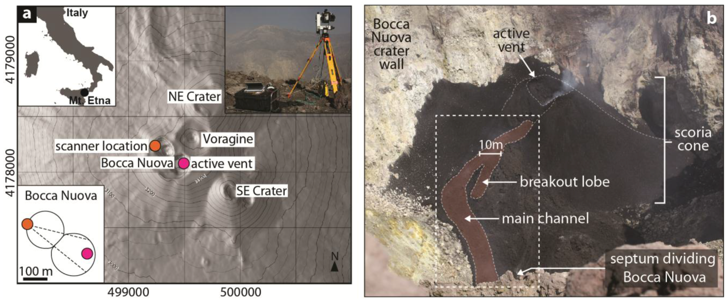
3. Data Acquisition and Processing

On 17, 19 and 21 July, we deployed a Riegl LPM-321 TLS instrument on the western rim of the Bocca Nuova. The LPM-321 is a very long-range near-infrared laser scanner (905-nm laser wavelength), which has been shown capable of providing useful data from up to 3.5 km on Mt. Etna [24]. At the Bocca Nuova, the instrument was located ~350 m from and ~100 m above the active vent located on the floor of the crater (Figure 1); consequently, the long-range capability was not required, and data could be collected using the instrument’s “short range” setting (~1000 points per second). The observation site was selected because it was safe and accessible and provided a good view of the active vent, scoria cone and near-vent regions of the lava flow. However, the main lava flow front was obscured by a septum that divides the Bocca Nuova (Figure 1b), so it could not be included in observations. On all days, the full cone and adjacent crater walls were surveyed using an angular step-width of 0.036º, to give an approximate ground resolution of 0.5 m.

On 21 July, a breakout lobe was observed advancing from the main lava flow, so the cone survey was augmented by a time-series of repeated scans focused on the active lava stream (flow scan window, Figure 1b). Each scan took ~10 minutes to complete and was immediately repeated, so that the acquisition of 10 scans occurred between 14:07 and 15:47 UTC. Data were captured at an angular step-width of 0.036º, which, for the flow region, gave an approximate ground resolution of 0.3 m. In addition, a Canon EOS 500D camera with a fixed 200-mm lens was used to capture 30-second interval time-lapse images covering the near-vent regions of the active flow.

3.1. TLS Data Processing

With no requirement for accurate absolute geo-referencing, ground control targets with dGPS coordinates were not used. To co-register full-cone scans for comparison, the survey from 17 July was taken as a reference, and the co-registration of subsequent surveys was refined using areas of static topography (i.e., the crater walls) and the ICP multi-station-adjustment tool in Riegl’s Riscan Pro processing software. A similar approach was used to ensure accurate co-registration of each of the lava time-series surveys from 21 July. Although the scanner was not moved between the repeated flow scans, the oscillatory motion of the LPM-321 scan head can results in the instrument settling over time, so small registration adjustments are recommended to minimize any accumulation of error [34].

To determine volumetric changes, the nature of the topography (i.e., few near-vertical surfaces at the scales of interest) and the relatively homogenous data coverage enabled appropriate volumes to be derived by straightforward DEM subtraction. For the crater scans, DEMs were created by interpolating the TLS point cloud data over a 0.5-m resolution grid in QGIS software. For the flow-only scans (which covered an area relatively close to the scanner), a 0.3-m resolution was used. Prior to DEM differencing, results were cropped, so that only relevant areas were included within calculations.

Determination of the volumetric change enabled overall cone growth and lava flux into the breakout lobe to be assessed. However, a similar calculation of lava flux was not possible for the main flow, due to the flow front being obscured from view and, hence, the full flow area not being captured. Thus, to derive flux in the main channel, surface velocities were required in order to estimate the flow rheology and, hence, through modelling, calculate the flux. The relatively rapid evolution of the flow surface, combined with the spatial and temporal resolution of the TLS data, meant that 3D feature tracking could not be usefully used to derive surface velocities from the TLS data alone, so the data were integrated with the time-lapse photography for velocity calculations.

3.2. Time-Lapse Photography Processing

To determine lava flow surface velocities, feature displacements were tracked in the time-lapse image sequence using “Pointcatcher” (http://tinyurl/pointcatcher), a Matlab-based time-lapse analysis software [20]. Pointcatcher enables automated normalised cross-correlation feature tracking (such as used in many particle imaging velocimetry (PIV) approaches) or manual interactive tracking for difficult image sequences in which automated analysis fails. Most of the Bocca Nuova flow surfaces were 'a'ā lava, for which the surface comprises decimetre and larger blocks, which rotate and move against each other as the flow advances. Consequently, even over the 30-s intervals between successive images, the resulting changes in image texture presented substantial challenges for automated image matching approaches and meant that only manual tracking could be reliably achieved. Thus, a manual interactive tracking approach was used in which individual features were tracked over a number of images rather than just between image pairs.

After feature tracks were collected from the breakout flow and the main channel, the 2D pixel measurements were converted into 3D feature trajectories by re-projecting the image features onto the TLS-derived topography. To do this, the camera was first registered to the TLS coordinate system: using the known camera position (adjacent to the scanner), the camera orientation could be determined by projecting TLS data onto the image and adjusting the camera angles until the TLS data appeared best aligned with the image scene. Due to computer-based matching between image features and topographic data being extremely challenging, the alignment process was carried out manually, so it is not associated with formal error estimates.

3.3. Measurement Error

The cited precision of LPM-321 range measurements is 0.015 m, but this is unlikely to be representative of measurement repeatability over a highly irregular surface, such as the scoria cone and lava flow. Thus, to estimate vertical error between co-registered TLS surveys, the root mean square error (RMSE) between static terrain areas in successive pairs of flow DEMs was derived and the mean calculated. We use the result (~0.05 m) to characterize the vertical error in calculations of volumes and depths. Due to the ICP co-registration, horizontal accuracy is likely to be of similar magnitude, but horizontal measurement precision is limited by the DEM resolutions (0.3 or 0.5 m).

Error magnitudes for flow surface velocity measurements are more difficult to determine due to the number of steps involved and the non-linear nature of the re-projection process. To assess sensitivity to uncertainty in the camera registration, the camera orientation was offset by 0.1° (almost three scan lines) and point re-projections repeated. Due to the favourable imaging geometry, the effect on mean velocities was only ~1%. Each point is also associated with a tracking error; the expected error in manual feature tracking is ~1–2 pixels and the footprint of time-lapse image pixels ~0.02–0.03 m. Thus, with typical travel distances for tracked surface features of order 1–2 m, the error component of velocity estimations was assumed to be sufficiently small that it could be neglected.

We therefore characterize overall error for viscosity and effusion rate by calculating straightforward minima and maxima bounds based on uncertainties in channel width and flow thickness, for which we use ±0.6 m and ±0.05 m, respectively, as conservatively large values.

4. Results

A difficulty in discussing effusion rate measurements is their variability over time and space. We adopt standard terminology [2,11,53] in which the “instantaneous lava effusion rate” describes the lava volumetric flux at the vent, measured at a single point in time, and the “time-averaged discharge rate” (TADR) represents mean conditions over a specified duration. Away from the vent, lava may flow in different channels, each with its own value of local lava flux. Combining contributions from both lava effusion and explosively-erupted products leads to the “total” discharge rate. However, the densities of lava and other erupted deposits can differ significantly, so volumes must be converted to “dense rock equivalent” (DRE) values before meaningful combinations or comparisons can be made.

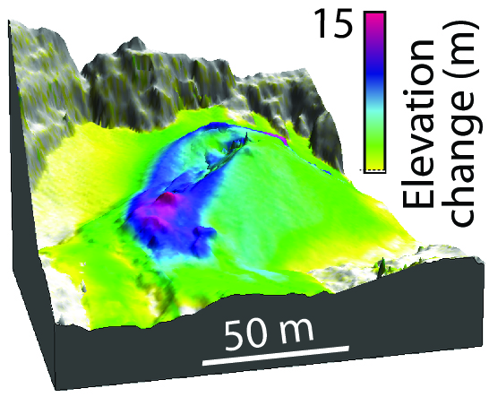
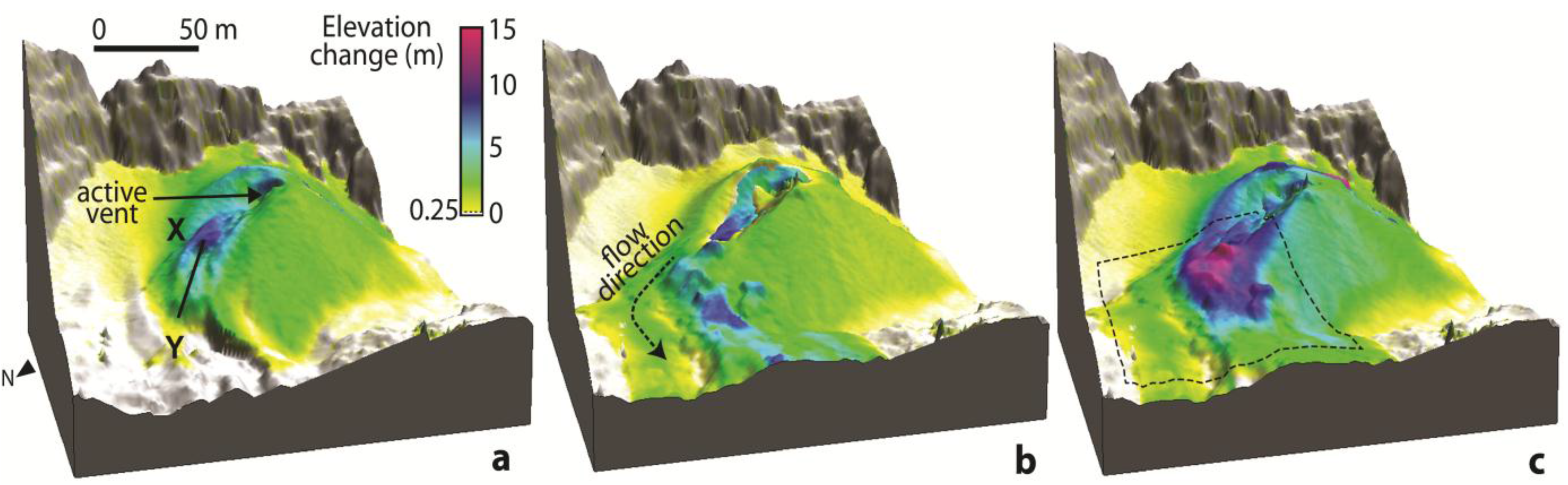
4.1. Cone Growth Rates 17–21 July

The three full-cone surveys enabled the growth of the cone to be assessed through DEM subtraction (Figure 2). Changes between the 17 and 19 July DEMs illustrate strong growth in the summit and northeastern regions (>10 m, Figure 2a), reflecting the relatively vigorous explosive activity over this period. Over the second period (19–21 July, Figure 2b), reduced explosive activity resulted in negligible summit growth and reduced growth of the cone flanks, but with extended lava emplacement in the northwest sector. The respective volumetric changes of ~4.7 × 10⁴ m³ and 3.7 × 10⁴ m³ for 17–19 July and 19–21 July give rates of ~0.15 m³·s⁻¹ DRE and ~0.10 m³·s⁻¹ DRE using an estimated 50% correction factor to account for clast vesicularity and packing density of the scoria (as used for similar work on Mt. Etna [54]). However, particularly for the second period, these values will represent minima due to the main flow front not being covered by the DEMs.

Figure 2. Elevation change in the full-cone DEMs for (a) 17–19 July, (b) 19–21 July and (c) 17–21 July. The perspective view is aligned looking southeast (as Figure 1b), with the lava flows in the foreground, effusing from a breach in the scoria cone. Sections of steep static topography in the background represent the lowest regions of the Bocca Nuova crater walls. In (c), the dashed outline illustrates the area of the DEM difference maps in Figure 3a.

Figure 2. Elevation change in the full-cone DEMs for (a) 17–19 July, (b) 19–21 July and (c) 17–21 July. The perspective view is aligned looking southeast (as Figure 1b), with the lava flows in the foreground, effusing from a breach in the scoria cone. Sections of steep static topography in the background represent the lowest regions of the Bocca Nuova crater walls. In (c), the dashed outline illustrates the area of the DEM difference maps in Figure 3a.

Figure 3. Elevation changes for the lava flow region from 10-minute repeat-interval TLS scans. (a) Difference maps with the active flow region delineated by the dashed lines (the region covered by the maps is illustrated by the dashed box in Figure 2c). The time marked on each panel denotes the time in-between the acquisitions of the differenced scans. In the panel labelled 15:37, the labelled sections are those in (b) (X-Y) and in Section 4.3 (X'-Y'). (b) Along-flow cross-sections between the points X and Y in (a), with the times given representing the midpoint times for each scan.

Figure 3. Elevation changes for the lava flow region from 10-minute repeat-interval TLS scans. (a) Difference maps with the active flow region delineated by the dashed lines (the region covered by the maps is illustrated by the dashed box in Figure 2c). The time marked on each panel denotes the time in-between the acquisitions of the differenced scans. In the panel labelled 15:37, the labelled sections are those in (b) (X-Y) and in Section 4.3 (X'-Y'). (b) Along-flow cross-sections between the points X and Y in (a), with the times given representing the midpoint times for each scan.

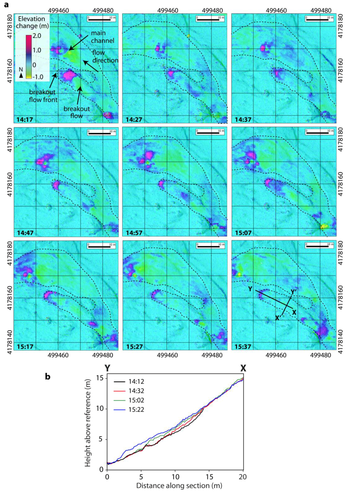
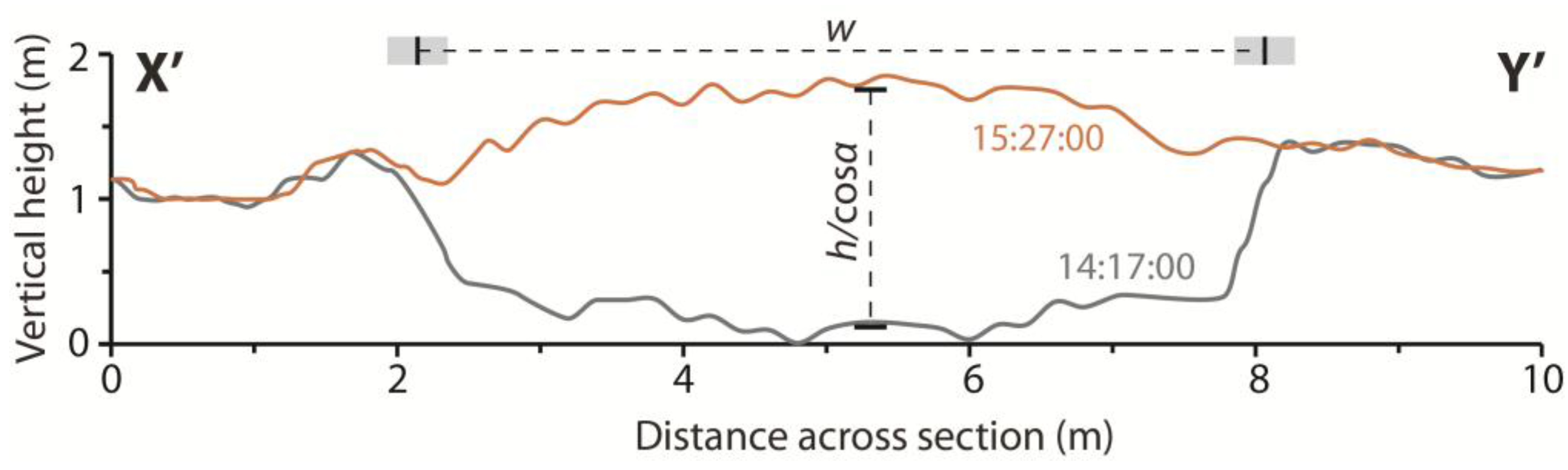
4.2. TLS-Based Time-Averaged Lava Discharge Rates, 21 July

The same DEM difference approach was adopted for quantifying lava emplacement alone from the TLS time series acquired on 21 July. Sequential DEM differences of the flow region clearly show down-flow progression of distinct topographic features in some areas, evidence for flow variability (pulses) and the advance of the breakout lobe flow front (Figure 3).

Focusing on the breakout lobe, the entirety of which is captured in the scans, indicates an advance rate of ~0.18 m·min⁻¹ and flow front thickening from ~0.4 m–0.8 m as it advances. Volumetric change gives estimated TADR values from sequential scans, which range between ~0.007 and 0.03 m³·s⁻¹ (Figure 4). The error on these values can be estimated by determining apparent volume changes over an equivalently-sized area (240 m²) of static topography. The root mean square of such volumes was 0.53 m, representing an uncertainty in the TADR values of ~0.0009 m³·s⁻¹. To estimate discharge rates for the main channel, for which the flow front is not covered by the DEMs, a model-based approach relying on measured surface velocities must be used.

Figure 4. Volumetric flux estimates for the breakout lobe. Time-averaged discharge rate (TADR) values are calculated from the elevation difference maps, with each line bracketing the entire start-to-end duration of the each scan pair used in the calculation. The estimated error in TADR is approximately the line thickness. The local effusion rate for the breakout flow lobe, Q_lobe (Section 4.3), is shown with the error bars illustrating the estimated minima and maxima bounds.

Figure 4. Volumetric flux estimates for the breakout lobe. Time-averaged discharge rate (TADR) values are calculated from the elevation difference maps, with each line bracketing the entire start-to-end duration of the each scan pair used in the calculation. The estimated error in TADR is approximately the line thickness. The local effusion rate for the breakout flow lobe, Q_lobe (Section 4.3), is shown with the error bars illustrating the estimated minima and maxima bounds.

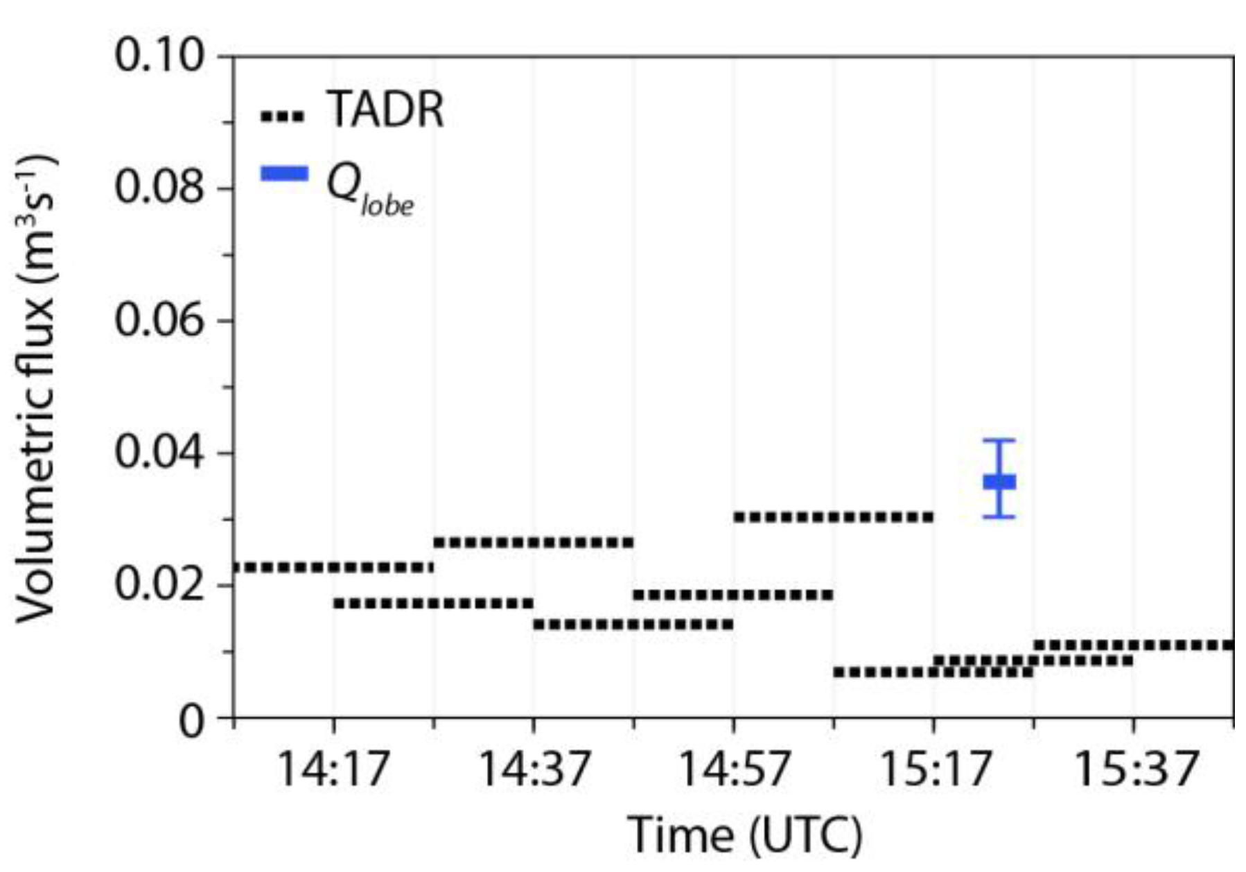
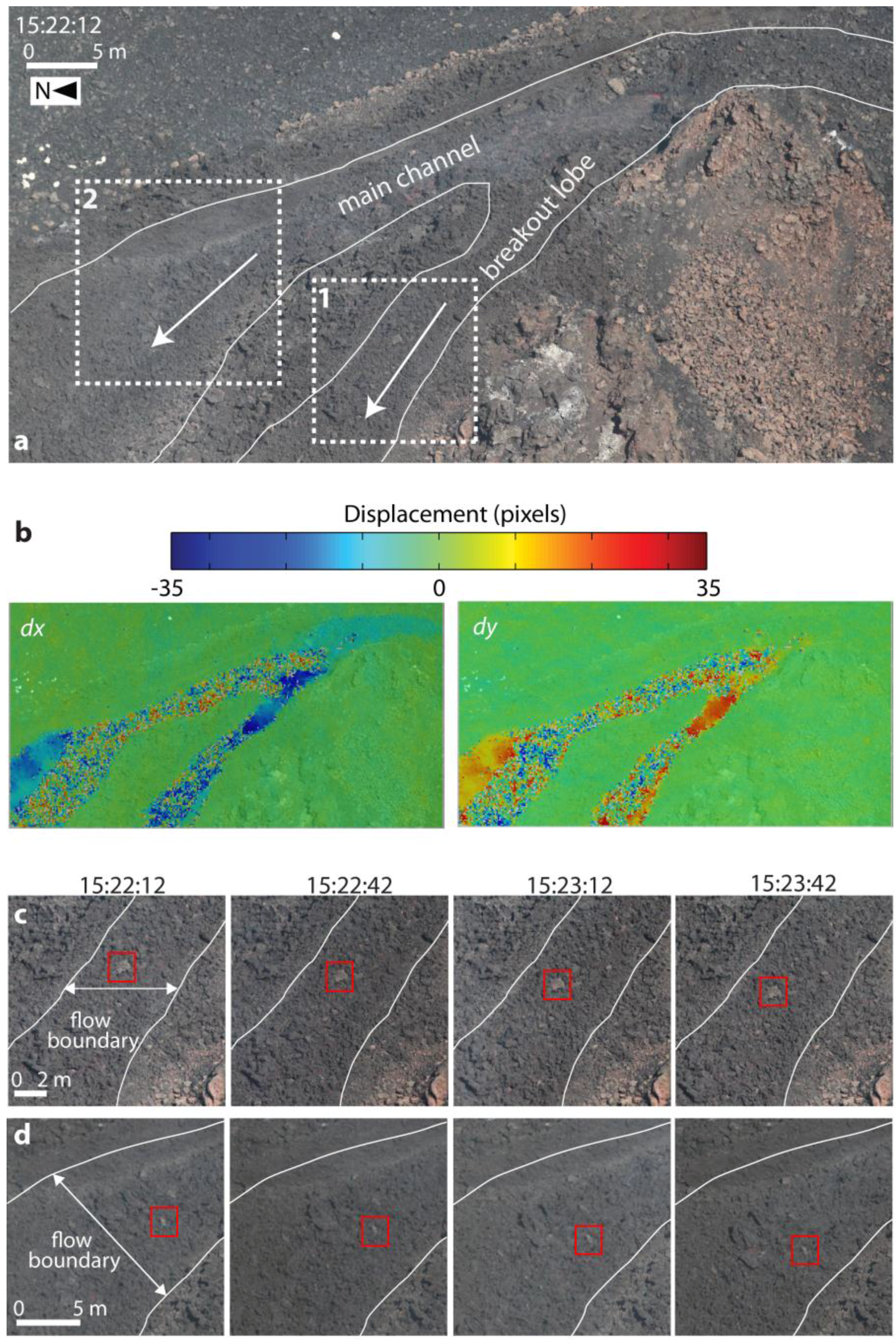
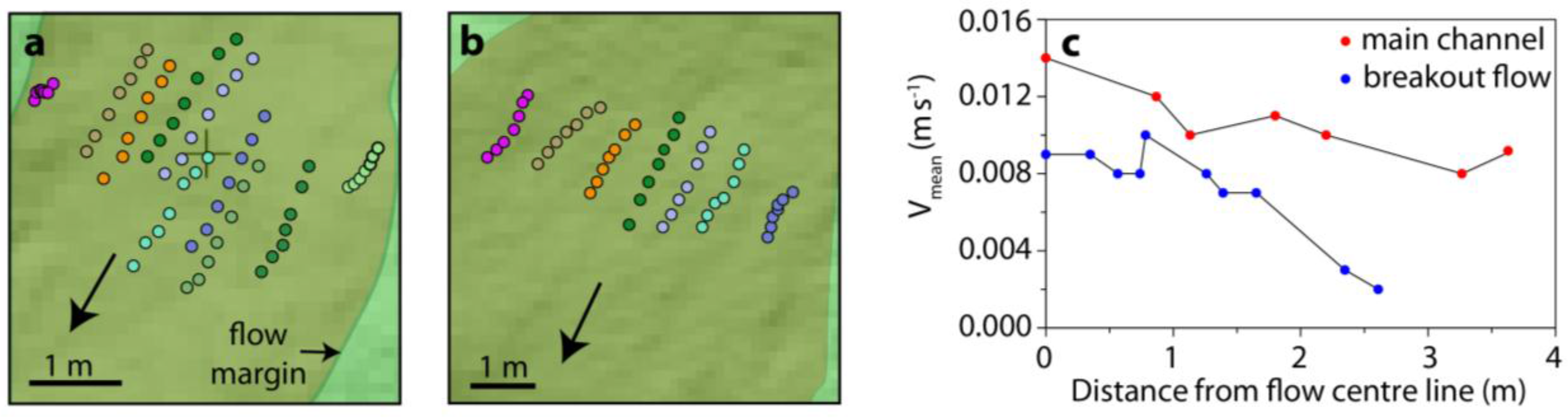
4.3. Image-Based Lava Viscosity and Instantaneous Effusion Rates

With a known surface velocity, flow models can be used to calculate lava flux given appropriate geometrical parameters (slope, cross-section flow dimensions and shape) and the lava’s rheology. For basaltic lavas in close proximity to the vent (such as in the Bocca Nuova) and where significant cooling has not yet occurred, it is typical to assume a near-Newtonian rheology [55,56]. This means that for the breakout lobe, the geometry of which can be fully defined from the TLS data, a flow viscosity can be derived. By using this value for the main flow, channel depth (which could not be otherwise constrained) can be estimated and, hence, a flux calculated.

For surface velocity measurements from the time-lapse images, weak image contrast and periods of obscuration by gas and condensing water vapour in the Bocca Nuova substantially limited the number of suitable images. Nevertheless, a set of seven successive images (15:22:12–15:25:12) were identified in which features could be successfully tracked on both the breakout flow lobe and the main channel (Figure 5).

Figure 5. Time-lapse images of the active flow. (a) A near-full image showing the areas used to determine flow velocity for the breakout flow (Box 1) and main channel (Box 2). (b) The results of automated pixel displacement analysis using a particle image velocimetry (PIV) approach (covering the area shown in (a) for the 15:22:12–15:22:42 image pair, analysed using PIVlab v1.4 [57,58]), split into x- and y-displacement components. Regions of smooth colour represent successful image matching; speckled areas indicate regions of noise where the matching has failed to track the flow surface movement. Extracts from the image sequence are shown for (c) the Region 1 and (d) the Region 2 areas displayed in (a), with the red boxes highlighting typical surface features that can be tracked with interactive techniques. Approximate scales are given for reference.

Figure 5. Time-lapse images of the active flow. (a) A near-full image showing the areas used to determine flow velocity for the breakout flow (Box 1) and main channel (Box 2). (b) The results of automated pixel displacement analysis using a particle image velocimetry (PIV) approach (covering the area shown in (a) for the 15:22:12–15:22:42 image pair, analysed using PIVlab v1.4 [57,58]), split into x- and y-displacement components. Regions of smooth colour represent successful image matching; speckled areas indicate regions of noise where the matching has failed to track the flow surface movement. Extracts from the image sequence are shown for (c) the Region 1 and (d) the Region 2 areas displayed in (a), with the red boxes highlighting typical surface features that can be tracked with interactive techniques. Approximate scales are given for reference.

PIV analysis of image pairs illustrated the limitations of using automated approaches on difficult imagery (Figure 5b). Although some areas of the active flows were matched successfully (e.g., the region prior to the channel bifurcation, top right, Figure 5b), most of the active surface was not, resulting in randomly-oriented displacement vectors, which were not representative of the flow. Thus, for reliable velocity estimation, manual feature tracking was required.

Features were selected across each channel to give across-flow velocity profiles (Figure 6, ten features on the breakout flow and seven on the main channel). To derive flux, channel shape and slope, flow width and thickness are required. For both the main channel and the breakout flow, channel width and slope can be measured directly from the imagery and TLS data. However, depth and channel shape cannot be directly measured for the main flow, because the pre-flow topography was not surveyed. Nevertheless, if a cross-sectional shape is assumed, an indirect estimate of depth can be made if flow rheology is known, and this could be derived from the breakout flow.

Figure 6. Flow feature displacements and mean surface velocities. Planimetric views of the re-projected point tracks on (a) the breakout flow and (b) the main channel (Regions 1 and 2 in Figure 5a). (c) The calculated mean velocities from the point displacements.

Figure 6. Flow feature displacements and mean surface velocities. Planimetric views of the re-projected point tracks on (a) the breakout flow and (b) the main channel (Regions 1 and 2 in Figure 5a). (c) The calculated mean velocities from the point displacements.

For the breakout flow, cross-sections through the original and the active flow surface show that it was travelling down a pre-existing channel (Figure 7), enabling the flow geometry to be reasonably represented with a rectangular cross-section of thickness, h, and width, w.

Figure 7. Vertical profiles through two DEMs demonstrating the topographic change due to the advance of the breakout flow lobe down an existing channel. The section is perpendicular to the planimetric direction of flow (Figure 3a) and labelled with the width and height values used to derive viscosity. Grey bars represent the inferred measurement uncertainty, but are too small to be visible in the vertical direction.

Figure 7. Vertical profiles through two DEMs demonstrating the topographic change due to the advance of the breakout flow lobe down an existing channel. The section is perpendicular to the planimetric direction of flow (Figure 3a) and labelled with the width and height values used to derive viscosity. Grey bars represent the inferred measurement uncertainty, but are too small to be visible in the vertical direction.

For a maximum surface velocity, V_max, down a slope, α, and assuming a Newtonian fluid of density ρ, the fluid viscosity, μ, is given by [56]:

$$\mu =\frac{\rho g{h}^{2}sin\alpha }{2V_{max}}\times \beta$$

(1)

where $\beta =1- \frac{32}{{\pi }^3} {\displaystyle \sum }_{n=1,3,5\dots }^{\infty }\frac{1}{n^3}{(-1)}^{(n-1)/2} \text{sech}\frac{n\pi w}{4h}$. Integration of flow velocity over the channel cross-section [56] gives the instantaneous discharge rate, Q, where:

$$Q=\raisebox{1ex}{$4$}\!\left/ \!\raisebox{-1ex}{$3$}\right.V_{max}wh\frac{\gamma }{\beta }$$

(2)

and γ = $\frac{384}{{\pi }^5} \frac{h}{w} {\displaystyle \sum }_{n=1,3,5, \dots }^{\infty }\frac{1}{n^5} \text{tanh}\frac{n\pi w}{4h}$.

Thus, estimating a lava density of 2067 kg·m⁻³ (reflecting a vesicularity of 22% as measured from other eruptions at Etna [59,60]), Equations 1 and 2 can be used to calculate lava viscosity and flux for the breakout channel. Using the derived viscosity and retaining a rectangular channel shape, the main flow depth can then be estimated (via Equation 1) and, thus, the flux calculated (Equation (2)). Although assumptions in channel shape can have substantial effects on estimated fluxes [61], with prior knowledge of viscosity and surface velocity enabling a depth estimate, this sensitivity is theoretically reduced to a few percent. Nevertheless, the underpinning assumption of a Newtonian rheology remains, and the breakout flow’s domed surface profile (Figure 7) suggests this may be a limiting simplification. Summing the lava fluxes from the breakout and main flow (Table 1) and accounting for the vesicularity then gives an instantaneous lava effusion rate for the active vent of 0.11 (0.10–0.13) m³·s⁻¹ DRE.

Table 1. Breakout flow and main channel parameters.

	Breakout Flow	Main Channel
Flow width, w (m)	6.0 ± 0.6	10.0 ± 0.6
Flow thickness, h (m)	1.24 ± 0.05	1.48 (1.42–1.54) a
Maximum flow velocity, Vmax (m·s−1)	0.0096	0.014
Slope angle, α (degrees)	28	28
Newtonian viscosity, μ (Pa·s) b	7.4 (6.8–8.1) × 105
Instantaneous discharge rate, Q (m3·s−1)	0.036 (0.030–0.042) b	0.11 (0.10–0.13) a

^a Bracketed values give upper and lower bounds based on calculated viscosity and width ranges; ^b bracketed values give the upper and lower bounds, based on flow width and thickness ranges.

Table 1. Breakout flow and main channel parameters.

	Breakout Flow	Main Channel
Flow width, w (m)	6.0 ± 0.6	10.0 ± 0.6
Flow thickness, h (m)	1.24 ± 0.05	1.48 (1.42–1.54) a
Maximum flow velocity, Vmax (m·s−1)	0.0096	0.014
Slope angle, α (degrees)	28	28
Newtonian viscosity, μ (Pa·s) b	7.4 (6.8–8.1) × 105
Instantaneous discharge rate, Q (m3·s−1)	0.036 (0.030–0.042) b	0.11 (0.10–0.13) a

^a Bracketed values give upper and lower bounds based on calculated viscosity and width ranges; ^b bracketed values give the upper and lower bounds, based on flow width and thickness ranges.

5. Discussion

Although the 2012 eruption of the Bocca Nuova did not constitute a hazardous event in terms of Mt. Etna’s activity, it provided excellent opportunity to test TLS performance for measuring effusion and discharge rates in restricted environments, as well as to estimate the scoria cone growth rate. The measured discharge rates are substantially lower than those recorded in 1999 (during which average values ranged from 8.7–11.6 m³·s⁻¹), when the crater overflowed [13]. Nevertheless, during 1999, instantaneous effusion rate measurements varied from 0.23–25 m³·s⁻¹. From our measurements in 2012, the activity cannot be ascribed a definitive effusion or discharge rate due to variations through time and the mixed contribution of lava and pyroclastic material to the cone growth. However, our data indicate that average rates should lie between ~0.1 and ~0.2 m³·s⁻¹ DRE.

5.1. Scoria Cone Growth

The cone growth of 8.4 × 10⁴ m³ characterized by mild Strombolian activity over the four-day measurement interval implies an average growth rate of ~0.12 m³·s⁻¹ DRE for that period, with emplacement slowing by ~30% between the first and last two days. When compared to recent much more violent events, it is much slower than the recent growth of the New Southeast Crater, which has grown episodically at ~50 m³·s⁻¹ during powerful lava fountaining eruptive episodes in 2011–2013 [54]. By comparison, the 2002 Laghetto cone was emplaced over 15 days of mixed Strombolian, phreatomagmatic and lava fountaining activity at an average rate of ~1.5 m³·s⁻¹ DRE [48], and the average growth rate of the Northeast Crater during its initial 60 years of life has been estimated at ~0.0005 m³·s⁻¹ [50]. Nevertheless, the Bocca Nuova cone grew at the same order of magnitude as short-term rates measured at other volcanoes, e.g., Izu–Oshima (0.9 m³·s⁻¹, 1986 [47]) La Fossa cone, Vulcano (0.2 m³·s⁻¹, 1888–1990 [62]) and Ngaurouhoe (0.65 m³·s⁻¹, 1954–1955 [63]).

5.2. Lava Emplacement and Rheology

The LPM-321 is optimized for very long range, rather than rapid measurement. Consequently, for the lava flow, the relatively slow scan speed (with scans taking ~10 minutes to complete) will have led to some apparent distortion of moving areas within the DEMs. However, through repeating scans by using identical acquisition parameters, there will be a negligible effect on volumetric changes calculated from difference DEMs, and they can be considered to represent time-averaged values.

Lava rheology is very difficult to measure directly in the field due to the hazards and temperatures involved, but forms an important input into the sophisticated numerical models used to forecast maximum flow lengths and extents. Thus, estimates made from recorded flow surface velocities and channel geometries form a valuable contribution to hazard assessments, and necessarily, they often assume a Newtonian rheology due to the scarcity of available measurements. However, although flow widths are generally straightforward to ascertain, measurements of depth are typically very poorly known (if channels drain, then depths can be observed [13,15,37]). Alternatively, as for the breakout flow here, flow fronts can be monitored and, thus, the pre-existing topography determined [15,19,20]. Thus, with a known cross-section and the ability to compare velocity-based model output to that from differences between TLS-derived DEMs, our results are unusually well constrained for field data. Our rheological measurements sit within the range of previous observations at Mt. Etna, e.g., viscosities between ~1.4 × 10⁴ Pa·s [64] in near-vent regions and up to ~10⁶ Pa·s for channels multiple kilometres from the vent [15]. Our time-lapse flow DEMs also provide options for further work, such as using the flow thickening to constrain rheological change through detailed flow modelling, in conjunction with thermal data.

5.3. Comparisons with Satellite-Derived Results

During the 2012 Bocca Nuova activity, TADR estimates were also being automatically generated by the HOTSAT volcano monitoring system [65] (Figure 8). HOTSAT uses infrared satellite data from MODIS and SEVIRI, but due to the small area involved during this eruptive activity, thermal anomalies were not detected by SEVIRI, indicating that the thermal activity was always less than ~100 MW per pixel (the minimum detectable radiative power [66]). Nevertheless, 21 nighttime July MODIS acquisitions showed thermally-anomalous pixels (Figure 8).

Figure 8. MODIS-derived TADR and cumulative erupted volume estimates. The dashed vertical lines indicate the acquisition start times of the TLS cone scans, and the grey bar represents the range of the TLS-derived TADR values (Figure 4).

Figure 8. MODIS-derived TADR and cumulative erupted volume estimates. The dashed vertical lines indicate the acquisition start times of the TLS cone scans, and the grey bar represents the range of the TLS-derived TADR values (Figure 4).

Although each satellite image is acquired effectively instantaneously, the processed results reflect time-averaged discharge values, rather than instantaneous effusion rates, because the spectral radiance from the entire flow field is used [8,67]. In the case of the Bocca Nuova, caution is further required when converting from radiated thermal energy to TADR due to the insulating conditions at the base of the ~100 m-deep crater. The enclosed environment is expected to result in substantial ambient temperature increases, which affect the relationship between radiative and convective heat losses from the flow and TADR estimates. To try and account for this, we use conversion parameter values that are generally applied to well-insulated flows [68] and derive a DRE TADR time series with a maximum value of 0.66 m³·s⁻¹ (16 July) and an average of 0.17 m³·s⁻¹ (Figure 8).

This average value is not too dissimilar from the instantaneous effusion rate of ~0.11 m³·s⁻¹ DRE inferred from TLS and time-lapse image measurements on 21 July. However, integrating the HOTSAT estimates that cover the duration of our field campaign gives an emplaced lava volume of ~1.1 × 10⁵ m³ over 120 h, representing a mean TADR of ~0.26 m³·s⁻¹ DRE, which is more than twice the ground-based results. Overestimation in the satellite data is also suggested by consideration of the MODIS-derived TADRs between 4 July and 4 August, which give a cumulative volume of ~2.6 × 10⁵ m³. This would represent an average lava thickness of ~15 m over the entire crater area (~1.7 × 10⁴ m²) that was not observed. It is probable that the bias towards overestimates reflect error in the radiance conversion parameters and relatively large magnitude radiance contributions from the vent itself and possibly also from pyroclastic deposits; similar factors have been inferred as responsible for the variation in detected radiance during periods of Strombolian activity at Stromboli [69]. It is likely that such errors could have been reduced if additional ground-based effusion rate estimates could have been made, which would have enabled conversion parameters to be calibrated specifically for the Bocca Nuova.

5.4. Use of TLS and Time-Lapse Photography during Future and Larger Eruptions

Ground-based time-lapse imagery is being increasingly collected as part of routine volcano monitoring, as well as in specific campaigns. For imagery to be suitable for deriving flow properties from automated analyses, matching algorithms must be able to reliably identify patches of image texture in different images. Texture depends on the contrast in the scene, the scales over which it varies and imaging parameters, such as the viewing distance, lens characteristics and camera resolution. Texture changes that hinder matching (such as that due to the evolving nature of the surface) can be reduced by imaging at higher temporal or lower spatial resolutions (e.g., more frequent images from longer distances). However, this impacts the theoretical measurement precision, and factors, such as heat shimmer, may also become important sources of noise. If available, thermal imagery can be used to provide much stronger texture than visible imagery, but usually at nearly an order of magnitude lower spatial resolution. Thus, where automated analyses fail, interactive approaches can be used to deliver displacements, and error can be reduced by feature tracking over multiple frames.

For TLS use, the Bocca Nuova activity represented an opportunity for which a mixed effusive and explosive eruption could be observed from a safe location with a relatively high angle view. In the case of more hazardous activity associated with greater effusion rates, such close-range measurements would not be possible, and longer-range, more oblique views (increasingly affected by occlusions) are likely. This could favour airborne data collection, if flights were possible (and could be funded). However, overflights are seldom sufficiently frequent to assess flow dynamics, and the multiple LiDAR acquisitions of Favalli et al. [37], at intervals down to ~15 minutes, represent a highly unique dataset.

At Mt. Etna, the most recent lavas have flowed into the Valle del Bove (up to ~6 km wide), where they can be overlooked from the valley sides and can be measured with the LPM-321 [24]. The associated pyroclastic cone (New Southeast Crater) can also be viewed from safe locations. More modern very long-range TLS systems offer extended range performance and significantly increased acquisition speeds, thus representing good opportunities for monitoring the emplacement of substantial lava flows and cones. For example, over a range of ~3500 m, a modern very long-range scanner may be capable of returning 30,000 points per second, with a laser footprint of ~0.4 m and a minimum point spacing of ~0.12 m. These greater speeds and higher spatial resolutions will enhance options for feature tracking in datasets and may facilitate lava surface velocity measurements from TLS data alone. Instrument performance under conditions involving strong degassing (which hinders data collection by droplets in condensing plumes giving false returns and creating occlusions) will also be of significant interest. Thus, as observation distances increase, so will challenges associated with data quality, and data cleaning and software-based optimization of scan position [70] will prove valuable tools for maximizing useful data returns.

TLS campaigns can add valuable constraints, both directly and indirectly, to other remote sensing techniques. For integration with ground-based time-lapse imagery (visible or thermal), single acquisitions may provide sufficient topographic data to aid analysis and image rectification. Time-lapse imagery can then be used to provide high spatial and temporal resolution quantitative data for change detection. However, for calibrating TADR estimates from satellite data in difficult environments, multiple TLS-TADR measurements are required, which should be well synchronized with some of the satellite acquisitions. Although this may be possible using campaign-style deployments, it would be easier if a permanent instrument installation were available. Very long-range measurement capability may make this a practical consideration in some cases and would also provide substantial improvements in instrument stability to facilitate small-scale change detection for deformation measurement and collapse forecasting.

6. Conclusions

Our study of the Bocca Nuova crater, Mt. Etna, presents the first use of TLS for constraining effusion and discharge rates for mixed effusive and explosive eruptive activity. Total discharge rates of ~0.1–0.2 m³·s⁻¹ DRE were recorded, with the range reflecting variability through time and the difficulties in separating contributions from lava flow and pyroclastic cone growth. The average emplacement rate of the cinder cone during its mild Strombolian activity over four observed days was ~0.12 m³·s⁻¹ DRE. This is in between the ~50 m³·s⁻¹ growth of the New Southeast Crater from lava fountaining [54] and the very low growth rate of the NE Crater during its first 60 years of mild Strombolian activity, estimated at ~0.0005 m³·s⁻¹ [50]. Integrating TLS surveys of active lava flows (acquired at 10-minute intervals) with time-lapse photography enabled simultaneous estimates of time-averaged lava discharge, instantaneous surface velocities and effusion rate and rheology. The enclosed environment of the Bocca Nuova and relatively mild nature of the eruption are challenges for deriving accurate discharge measurements from satellite data and likely result in overestimates. Thus, our results demonstrate the potential of TLS for characterizing active volcanic processes and their associated hazards and for supporting the interpretation of other remote sensing approaches.

References

1. Blong, R.J. Volcanic Hazards; Academic Press Australia: North Ryde, NSW, Australia, 1984. [Google Scholar]
2. Walker, G.P.L.; Huntingdon, A.T.; Sanders, A.T.; Dinsdale, J.L. Lengths of lava flows. Phil. Trans. R. Soc. Lond. A. 1973, 274, 107–118. [Google Scholar] [CrossRef]
3. Harris, A.; Steffke, A.; Calvari, S.; Spampinato, L. Thirty years of satellite-derived lava discharge rates at Etna: Implications for steady volumetric output. J. Geophys. Res. 2011, 116. [Google Scholar] [CrossRef]
4. Bonaccorso, A.; Calvari, S. Major effusive eruptions and recent lava fountains: Balance between expected and erupted magma volumes at Etna volcano. Geophys. Res. Lett. 2013, 40, 6069–6073. [Google Scholar] [CrossRef]
5. Coppola, D.; Piscopo, D.; Staudacher, T.; Cigolini, C. Lava discharge rate and effusive pattern at Piton de la Fournaise from MODIS data. J. Volcanol. Geotherm. Res. 2009, 184, 174–192. [Google Scholar] [CrossRef]
6. Harris, A.J.L.; Butterworth, A.L.; Carlton, R.W.; Downey, I.; Miller, P.; Navarro, P.; Rothery, D.A. Low-cost volcano surveillance from space: Case studies from Etna, Krafla, Cerro Negro, Fogo, Lascar and Erebus. Bull. Volcanol. 1997, 59, 49–64. [Google Scholar] [CrossRef]
7. Harris, A.J.L.; Baloga, S.M. Lava discharge rates from satellite-measured heat flux. Geophys. Res. Lett. 2009, 36. [Google Scholar] [CrossRef]
8. Wright, R.; Blake, S.; Harris, A.J.L.; Rothery, D.A. A simple explanation for the space-based calculation of lava eruption rates. Earth Planet. Sci. Lett. 2001, 192, 223–233. [Google Scholar] [CrossRef]
9. Ganci, G.; James, M.R.; Calvari, S.; Del Negro, C. Separating the thermal fingerprints of lava flows and simultaneous lava fountaining using ground-based thermal camera and SEVIRI measurements. Geophys. Res. Lett. 2013, 40, 5058–5063. [Google Scholar] [CrossRef]
10. Coppola, D.; James, M.R.; Staudacher, T.; Cigolini, C. A comparison of field- and satellite-derived thermal flux at Piton de la Fournaise: Implications for the calculation of lava discharge rate. Bull. Volcanol. 2010, 72, 341–356. [Google Scholar] [CrossRef]
11. Lipman, P.W.; Banks, N.G. 'A'ā flow dynamics, Mauna Loa 1984. In Volcanism in Hawaii; Decker, R.W., Wright, T.L., Stauffer, P.H., Eds.; U.S. Geological Survey: Reston, VA, USA, 1987; pp. 1527–1567. [Google Scholar]
12. Harris, A.J.L.; Murray, J.B.; Aries, S.E.; Davies, M.A.; Flynn, L.P.; Wooster, M.J.; Wright, R.; Rothery, D.A. Effusion rate trends at Etna and Krafla and their implications for eruptive mechanisms. J. Volcanol. Geotherm. Res. 2000, 102, 237–270. [Google Scholar] [CrossRef]
13. Calvari, S.; Neri, M.; Pinkerton, H. Effusion rate estimations during the 1999 summit eruption on Mount Etna, and growth of two distinct lava flow fields. J. Volcanol. Geotherm. Res. 2002, 119, 107–123. [Google Scholar] [CrossRef]
14. Bailey, J.E.; Harris, A.J.L.; Dehn, J.; Calvari, S.; Rowland, S.K. The changing morphology of an open lava channel on Mt. Etna. Bull. Volcanol. 2006, 68, 497–515. [Google Scholar] [CrossRef] [Green Version]
15. James, M.R.; Pinkerton, H.; Robson, S. Image-based measurement of flux variation in distal regions of active lava flows. Geochem. Geophys. Geosyst. 2007, 8. [Google Scholar] [CrossRef] [Green Version]
16. Harris, A.; Dehn, J.; Patrick, M.; Calvari, S.; Ripepe, M.; Lodato, L. Lava effusion rates from hand-held thermal infrared imagery: An example from the June 2003 effusive activity at Stromboli. Bull. Volcanol. 2005, 68, 107–117. [Google Scholar] [CrossRef]
17. Lautze, N.C.; Harris, A.J.L.; Bailey, J.E.; Ripepe, M.; Calvari, S.; Dehn, J.; Rowland, S.K.; Evans-Jones, K. Pulsed lava effusion at Mount Etna during 2001. J. Volcanol. Geotherm. Res. 2004, 137, 231–246. [Google Scholar] [CrossRef]
18. James, M.R.; Robson, S.; Pinkerton, H.; Ball, M. Oblique photogrammetry with visible and thermal images of active lava flows. Bull. Volcanol. 2006, 69, 105–108. [Google Scholar] [CrossRef]
19. Hamilton, C.W.; Glaze, L.S.; James, M.R.; Baloga, S. Topographic and stochastic influences on pāhoehoe lava lobe emplacement. J. Volcanol. Geotherm. Res. 2013, 75. [Google Scholar] [CrossRef]
20. James, M.R.; Robson, S. Sequential digital elevation models of active lava flows from ground-based stereo time-lapse imagery. ISPRS J. Photogramm. Remote Sens. 2014, 97, 160–170. [Google Scholar] [CrossRef]
21. Macfarlane, D.G.; Wadge, G.; Robertson, D.A.; James, M.R.; Pinkerton, H. Use of a portable topographic mapping millimetre wave radar at an active lava flow. Geophys. Res. Lett. 2006, 33. [Google Scholar] [CrossRef] [Green Version]
22. Wadge, G.; Saunders, S.; Itikarai, I. Pulsatory andesite lava flow at Bagana Volcano. Geochem. Geophys. Geosyst. 2012, 13. [Google Scholar] [CrossRef]
23. Poland, M.P. Time-averaged discharge rate of subaerial lava at Kilauea Volcano, Hawai’i, measured from TanDEM-X interferometry: Implications for magma supply and storage during 2011–2013. J. Geophys. Res. 2014, 119, 5464–5481. [Google Scholar] [CrossRef]
24. James, M.R.; Pinkerton, H.; Applegarth, L.J. Detecting the development of active lava flow fields with a very-long-range terrestrial laser scanner and thermal imagery. Geophys. Res. Lett. 2009, 36. [Google Scholar] [CrossRef]
25. Rabatel, A.; Deline, P.; Jaillet, S.; Ravanel, L. Rock falls in high-alpine rock walls quantified by terrestrial lidar measurements: A case study in the Mont Blanc area. Geophys. Res. Lett. 2008, 35. [Google Scholar] [CrossRef]
26. Abellan, A.; Vilaplana, J.M.; Calvet, J.; Garcia-Selles, D.; Asensio, E. Rockfall monitoring by Terrestrial Laser Scanning—Case study of the basaltic rock face at Castellfollit de la Roca (Catalonia, Spain). Nat. Hazards Earth Syst. Sci. 2011, 11, 829–841. [Google Scholar] [CrossRef]
27. Oppikofer, T.; Jaboyedoff, M.; Blikra, L.; Derron, M.H.; Metzger, R. Characterization and monitoring of the Aknes rockslide using Terrestrial Laser Scanning. Nat. Hazards Earth Syst. Sci. 2009, 9, 1003–1019. [Google Scholar] [CrossRef]
28. Teza, G.; Pesci, A.; Genevois, R.; Galgaro, A. Characterization of landslide ground surface kinematics from Terrestrial Laser Scanning and strain field computation. Geomorphology 2008, 97, 424–437. [Google Scholar] [CrossRef]
29. Prokop, A.; Panholzer, H. Assessing the capability of Terrestrial Laser Scanning for monitoring slow moving landslides. Nat. Hazards Earth Syst. Sci. 2009, 9, 1921–1928. [Google Scholar] [CrossRef]
30. Aryal, A.; Brooks, B.A.; Reid, M.E.; Bawden, G.W.; Pawlak, G.R. Displacement fields from point cloud data: Application of particle imaging velocimetry to landslide geodesy. J. Geophys. Res. 2012, 117. [Google Scholar] [CrossRef]
31. Gigli, G.; Morelli, S.; Fornera, S.; Casagli, N. Terrestrial laser scanner and geomechanical surveys for the rapid evaluation of rock fall susceptibility scenarios. Landslides 2014, 11, 1–14. [Google Scholar] [CrossRef]
32. Bauer, A.; Paar, G.; Kaufmann, V. Terrestrial laser scanning for rock glacier monitoring. In Proceedings of the 8th Infernational Conference on Permafrost, Zurich, Switzerland, 20–25 July 2003.
33. Schwalbe, E.; Maas, H.-G. Motion analysis of fast flowing glaciers from multi-temporal Terrestrial Laser Scanning. Photogramm. Fernerkund. Geoinf. 2009, 1, 91–98. [Google Scholar] [CrossRef]
34. Schwalbe, E.; Maas, H.-G.; Dietrich, R.; Ewert, H. Glacier velocity determination from multi-temporal long range laser scanner point clouds. In Proceedings of XXIst ISPRS Congress, Beijing, China, 3–11 July 2008.
35. Hunter, G.; Pinkerton, H.; Airey, R.; Calvari, S. The application of a long-range laser scanner for monitoring volcanic activity on Mount Etna. J. Volcanol. Geotherm. Res. 2003, 123, 203–210. [Google Scholar] [CrossRef]
36. Pesci, A.; Loddo, F.; Confort, D. The first terrestrial laser scanner application over Vesuvius: High resolution model of a volcano crater. Int. J. Remote Sens. 2007, 28, 203–219. [Google Scholar] [CrossRef]
37. Favalli, M.; Fornaciai, A.; Mazzarini, F.; Harris, A.; Neri, M.; Behncke, B.; Pareschi, M.T.; Tarquini, S.; Boschi, E. Evolution of an active lava flow field using a multitemporal LIDAR acquisition. J. Geophys. Res. 2010, 115. [Google Scholar] [CrossRef]
38. Jones, L.K.; Kyle, P.R.; Oppenheimer, C.; Frechette, J.D.; Okal, M.H. Terrestrial Laser Scanning observations of geomorphic changes and varying lava lake levels at Erebus volcano, Antarctica. J. Volcanol. Geotherm. Res. 2015, 295, 43–54. [Google Scholar] [CrossRef]
39. Scambos, T.A.; Dutkiewicz, M.J.; Wilson, J.C.; Bindschadler, R.A. Application of image cross-correlation to the measurement of glacier velocity using satellite image data. Remote Sens. Environ. 1992, 42, 177–186. [Google Scholar] [CrossRef]
40. Leprince, S.; Ayoub, F.; Klinger, Y.; Avouac, J.-P. Co-registration of optically sensed images and correlation (COSI-Corr): An operational methodology for ground deformation measurements. In Proceedings of 2007 IEEE International Geoscience and Remote Sensing Symposium (IGARSS), Barcelona, Spain, 23–28 July 2007.
41. Travelletti, J.; Delacourt, C.; Allemand, P.; Malet, J.P.; Schmittbuhl, J.; Toussaint, R.; Bastard, M. Correlation of multi-temporal ground-based optical images for landslide monitoring: Application, potential and limitations. ISPRS J. Photogramm. Remote Sens. 2012, 70, 39–55. [Google Scholar] [CrossRef]
42. James, M.R.; Applegarth, L.J.; Pinkerton, H. Lava channel roofing, overflows, breaches and switching: insights from the 2008–2009 eruption of Mt. Etna. Bull. Volcanol. 2012, 74, 107–117. [Google Scholar] [CrossRef]
43. Walter, T.R. Low cost volcano deformation monitoring: Optical strain measurement and application to Mount St. Helens data. Geophys. J. Int. 2011, 186, 699–705. [Google Scholar] [CrossRef]
44. Luhr, J.F.; Simkin, T. Paricutin, The volcano born in a Mexican Cornfield; Geoscience Press: Phoenix, AZ, USA, 1993; p. 427. [Google Scholar]
45. Yasui, M.; Koyaguchi, T. Sequence and eruptive style of the 1783 eruption of Asama Volcano, central Japan: A case study of an andesitic explosive eruption generating fountain-fed lava flow, pumice fall, scoria flow and forming a cone. Bull. Volcanol. 2004, 66, 243–262. [Google Scholar] [CrossRef]
46. Wolfe, E.W.; Neal, C.A.; Banks, N.G.; Duggan, T.J. Geologic Observations and Chronology of Eruptive Events; U.S. Geological Survey: Reston, VA, USA, 1988.
47. Sumner, J.M. Formation of clastogenic lava flows during fissure eruption and scoria cone collapse: The 1986 eruption of Izu-Oshima Volcano, eastern Japan. Bull. Volcanol. 1998, 60, 195–212. [Google Scholar] [CrossRef]
48. Calvari, S.; Pinkerton, H. Birth, growth and morphologic cinder cone during the evolution of the “Laghetto” 2001 Etna eruption. J. Volcanol. Geotherm. Res. 2004, 132, 225–239. [Google Scholar] [CrossRef]
49. Di Traglia, F.; Cimarelli, C.; de Rita, D.; Gimeno Torrente, D. Changing eruptive styles in basaltic explosive volcanism: Examples from Croscat complex scoria cone, Garrotxa Volcanic Field (NE Iberian Peninsula). J. Volcanol. Geotherm. Res. 2009, 180, 89–109. [Google Scholar] [CrossRef]
50. McGetchin, T.R.; Settle, M.; Chouet, B.A. Cinder cone growth modeled after Northeast Crater, Mount-Etna, Sicily. J. Geophys. Res. 1974, 79, 3257–3272. [Google Scholar] [CrossRef]
51. Houghton, B.F.; Schmincke, H.U. Rothenberg scoria cone, East Eifel—A complex strombolian and phreatomagmatic volcano. Bull. Volcanol. 1989, 52, 28–48. [Google Scholar] [CrossRef]
52. Neri, M.; Mazzarini, F.; Tarquini, S.; Bisson, M.; Isola, I.; Behncke, B.; Pareschi, M.T. The changing face of Mount Etna’s summit area documented with Lidar technology. Geophys. Res. Lett. 2008, 35. [Google Scholar] [CrossRef]
53. Harris, A.J.L.; Dehn, J.; Calvari, S. Lava effusion rate definition and measurement: A review. Bull. Volcanol. 2007, 70, 1–22. [Google Scholar] [CrossRef]
54. Behncke, B.; Branca, S.; Corsaro, R.A.; De Beni, E.; Miraglia, L.; Proietti, C. The 2011–2012 summit activity of Mount Etna: Birth, growth and products of the new SE crater. J. Volcanol. Geotherm. Res. 2014, 270, 10–21. [Google Scholar] [CrossRef]
55. Pinkerton, H.; Stevenson, R.J. Methods of determining the rheological properties of magmas at sub-liquidus temperatures. J. Volcanol. Geotherm. Res. 1992, 53, 47–66. [Google Scholar] [CrossRef]
56. Tallarico, A.; Dragoni, M. Viscous Newtonian laminar flow in a rectangular channel: Application to Etna lava flows. Bull. Volcanol. 1999, 61, 40–47. [Google Scholar] [CrossRef]
57. Thielicke, W. The Flapping Flight of Birds—Analysis and Application. PhD Thesis, Rijksuniversiteit Groningen, Groningen, Netherlands, 2014. [Google Scholar]
58. Thielicke, W.; Stamhuis, E.J. PIVlab—Towards user-friendly, affordable and accurate digital particle image velocimetry in MATLAB. J. Open Res. Software 2014, 2. [Google Scholar] [CrossRef]
59. Gaonach, H.; Stix, J.; Lovejoy, S. Scaling effects on vesicle shape, size and heterogeneity of lavas from Mount Etna. J. Volcanol. Geotherm. Res. 1996, 74, 131–153. [Google Scholar] [CrossRef]
60. Herd, R.A.; Pinkerton, H. Bubble coalescence in basaltic lava: Its impact on the evolution of bubble populations. J. Volcanol. Geotherm. Res. 1997, 75, 137–157. [Google Scholar] [CrossRef]
61. Lev, E.; James, M.R. The influence of cross-sectional channel geometry on rheology and flux estimates for active lava flows. Bull. Volcanol. 2014, 76. [Google Scholar] [CrossRef]
62. Di Traglia, F.; Pistolesi, M.; Rosi, M.; Bonadonna, C.; Fusillo, R.; Roverato, M. Growth and erosion: The volcanic geology and morphological evolution of La Fossa (Island of Vulcano, Southern Italy) in the last 1000 years. Geomorphology 2013, 194, 94–107. [Google Scholar] [CrossRef]
63. Hobden, B.J.; Houghton, B.F.; Nairn, I.A. Growth of a young, frequently active composite cone: Ngauruhoe Volcano, New Zealand. Bull. Volcanol. 2002, 64, 392–409. [Google Scholar] [CrossRef]
64. Pinkerton, H.; Norton, G. Rheological properties of basaltic lavas at sub-liquidus temperatures: Laboratory and field-measurements on lavas from Mount Etna. J. Volcanol. Geotherm. Res. 1995, 68, 307–323. [Google Scholar] [CrossRef]
65. Ganci, G.; Vicari, A.; Fortuna, L.; Del Negro, C. The HOTSAT volcano monitoring system based on combined use of SEVIRI and MODIS multispectral data. Ann. Geophys. 2011, 54, 544–550. [Google Scholar]
66. Roberts, G.; Wooster, M.J.; Perry, G.L.W.; Drake, N.; Rebelo, L.M.; Dipotso, F. Retrieval of biomass combustion rates and totals from fire radiative power observations: Application to southern Africa using geostationary SEVIRI imagery. J. Geophys. Res. 2005, 110, D21111. [Google Scholar] [CrossRef]
67. Garel, F.; Kaminski, E.; Tait, S.; Limare, A. An experimental study of the surface thermal signature of hot subaerial isoviscous gravity currents: Implications for thermal monitoring of lava flows and domes. J. Geophys. Res. 2012, 117, B02205. [Google Scholar] [CrossRef]
68. Harris, A.; Favalli, M.; Steffke, A.; Fornaciai, A.; Boschi, E. A relation between lava discharge rate, thermal insulation, and flow area set using lidar data. Geophys. Res. Lett. 2010, 37, L20308. [Google Scholar] [CrossRef]
69. Coppola, D.; Piscopo, D.; Laiolo, M.; Cigolini, C.; Delle Donne, D.; Ripepe, M. Radiative heat power at Stromboli volcano during 2000–2011: Twelve years of MODIS observations. J. Volcanol. Geotherm. Res. 2012, 215, 48–60. [Google Scholar] [CrossRef]
70. Slatcher, N. Application and Optimisation of Terrestrial Laser Scanners for Geohazard Assessment. PhD Thesis, Lancaster University, Lancaster, UK, 2015. [Google Scholar]