Evaluation of Six Algorithms to Monitor Wheat Leaf Nitrogen Concentration

Abstract

The rapid and non-destructive monitoring of the canopy leaf nitrogen concentration (LNC) in crops is important for precise nitrogen (N) management. Nowadays, there is an urgent need to identify next-generation bio-physical variable retrieval algorithms that can be incorporated into an operational processing chain for hyperspectral satellite missions. We assessed six retrieval algorithms for estimating LNC from canopy reflectance of winter wheat in eight field experiments. These experiments represented variations in the N application rates, planting densities, ecological sites and cultivars and yielded a total of 821 samples from various places in Jiangsu, China over nine consecutive years. Based on the reflectance spectra and their first derivatives, six methods using different numbers of wavelengths were applied to construct predictive models for estimating wheat LNC, including continuum removal (CR), vegetation indices (VIs), stepwise multiple linear regression (SMLR), partial least squares regression (PLSR), artificial neural networks (ANNs), and support vector machines (SVMs). To assess the performance of these six methods, we provided a systematic evaluation of the estimation accuracies using the six metrics that were the coefficients of determination for the calibration (R²_C) and validation (R²_V) sets, the root mean square errors of prediction (RMSE_P) for the calibration and validation sets, the ratio of prediction to deviation (RPD), the computational efficiency (CE) and the complexity level (CL). The following results were obtained: (1) For the VIs method, SAVI(R₁₂₀₀, R₇₀₅) produced a more accurate estimation of the LNC than other indices, with R²_C, R²_V, RMSE_P, RPD and CE values of 0.844, 0.795, 0.384, 2.005 and 0.10 min, respectively; (2) For the SMLR, PLSR, ANNs and SVMs methods, the SVMs using the first derivative canopy spectra (SVM-FDS) offered the best accuracy in terms of R²_C, R²_V, RMSE_P, RPD, and CE, at 0.96, 0.78, 0.37, 2.02, and 21.17, respectively; (3) The PLSR-FDS, ANN-OS and SVM-FDS methods yield similar accuracies if the CE and CL are not considered, however, ANNs and SVMs performed better on calibration set than the validation set which indicate that we should take more caution with the two methods for over-fitting. Except PLS method, the performance for most methods did not enhance when the spectrum were operated by the first derivative. Moreover, the evaluation of the robustness demonstrates that SVM method may be better suited than the other methods to cope with potential confounding factors for most varieties, ecological site and growth stage; (4) The prediction accuracy was found to be higher when more wavelengths were used, though at the cost of a lower CE. The findings are of interest to the remote sensing community for the development of improved inversion schemes for hyperspectral applications concerning other types of vegetation. The examples provided in this paper may also serve to illustrate the advantages and shortcomings of empirical hyperspectral models for mapping important vegetation biophysical properties of other crops.

1. Introduction

In cereal crops, nitrogen (N) is the most important element for maintaining growth status and enhancing grain yield [1]. Therefore, the real-time, nondestructive and accurate monitoring of the nitrogen (N) concentration in crops has become a key technique for timely diagnosis of problems, precise fertilization and productivity estimation [2,3,4,5,6,7,8,9,10]. Remote sensing has been widely applied in recent decades to determine the biophysical and chemical parameters of crops [2,11,12]. Many forthcoming hyperspectral satellite missions will be dedicated to land and crop monitoring. Hence, there is an urgent need to identify next-generation bio-geophysical variable retrieval algorithms that can be incorporated into an operational processing chain.

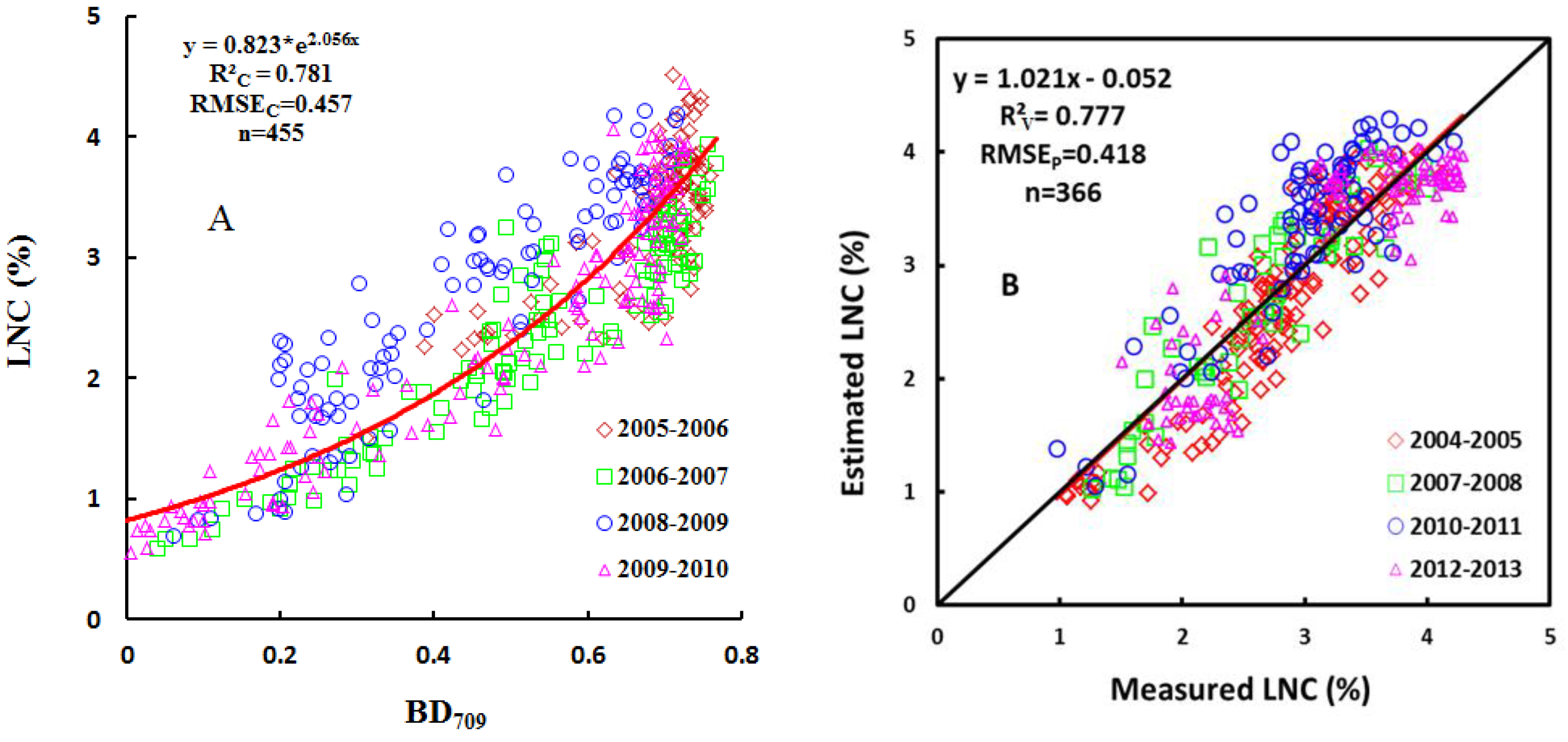
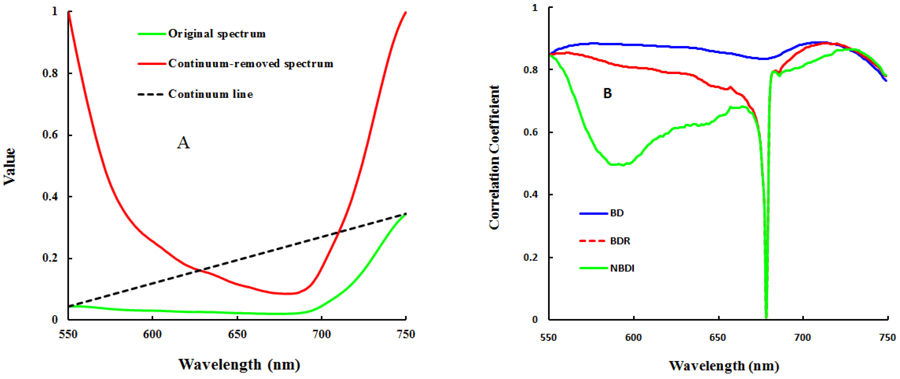
Considerable progress has been made using multispectral and hyperspectral data acquired from ground and aerial platforms to estimate the N concentration of crops [8,13,14,15,16,17,18,19]. Existing reports indicate that in most previous work, the core wavelengths have first been determined and then used to construct a sensitive spectral index, as in the case of the continuum removal (CR) and the vegetation index (VI) method. The CR method can be used to effectively isolate individual absorption features of interest and estimate the chemical concentration in dried leaves [20,21,22]. 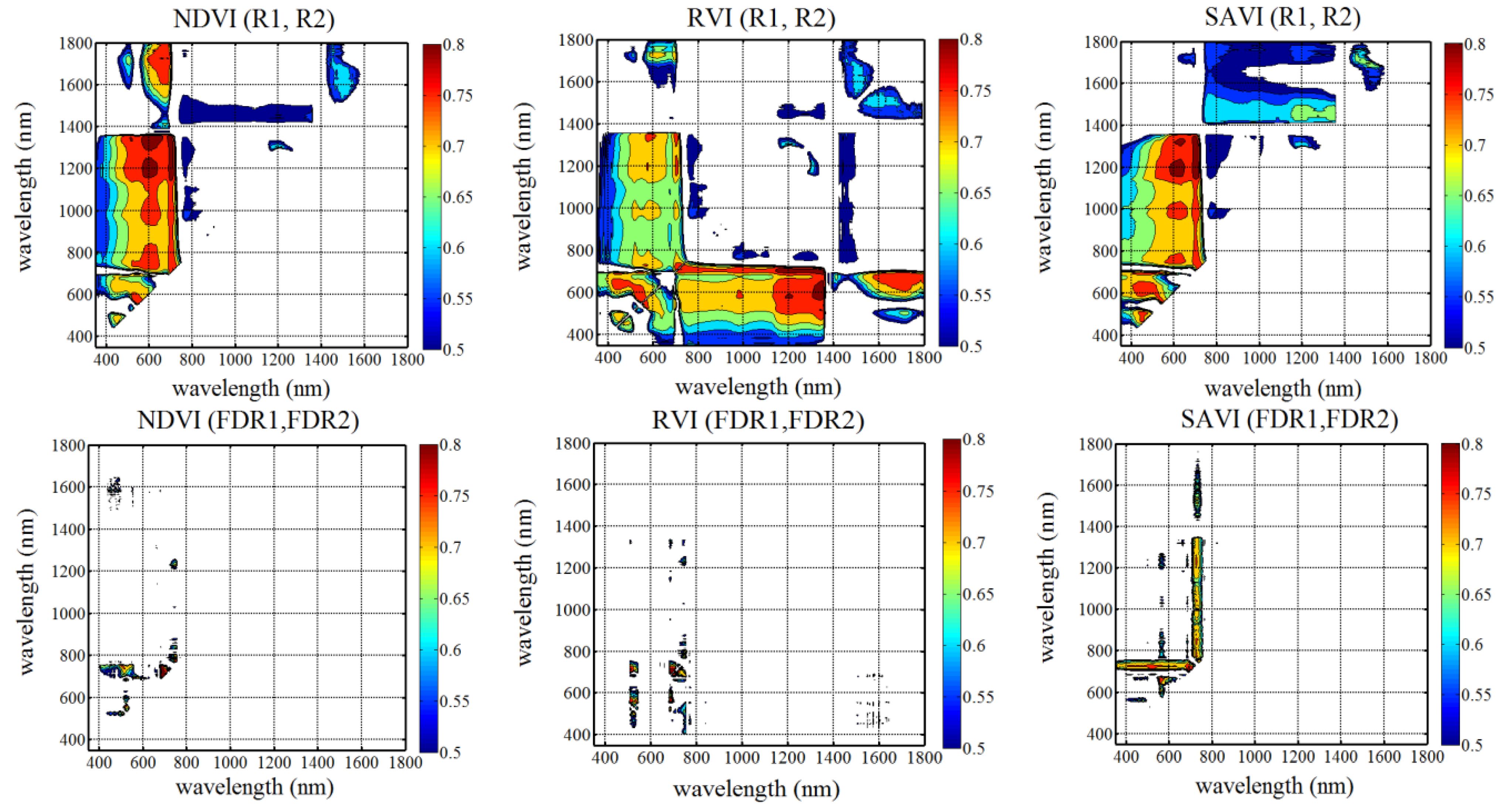However, one must determine the spectral range each time when the CR operation is performed, which results in unstable performance in monitoring of the chemical concentration of crops [23]. In addition to the CR method, various vegetation indices, such as the Normalized Difference Vegetation Index (NDVI), the Ratio Vegetation Index (RVI), the Soil-Adjusted Vegetation Index (SAVI), Modified Normalized Difference (mND), and the Photochemical Reflectance Index (PRI), have been widely used to characterize chemical concentration of plants because these indices have simple forms and are easy to calculate [10,12,24,25,26]. However, most researchers use only a limited number of wavelengths in specific spectral regions to calculate these indices and have not exploited the full spectrum information in hyperspectral data. In addition, many of these vegetation indices are strongly influenced by the soil background, resulting in soil-dependent VI-biophysical relationships. Linear regression models are typically analyzed based on individual input variables of the characteristic wavelength or vegetation index. Therefore, several researchers have suggested that multivariable input parameters should be considered when constructing such linear regressions.

Presently, the commercial instruments that are used to monitor crop N concentrations, such as ASD [27] and hyperspectral imager, are not suitable for future use on family farms or for individual users because of their high cost and relatively complex operational procedures. A number of other portable devices, such as the SPAD (650 and 940 nm) [28], can only work on a single leaf each time and therefore cannot be applied to large populations of plants. The LNC models that are currently developed with specific wavelengths on portable devices, such as the GreenSeeker (656 and 770 nm) and the Crop Circle (450,550,650,670,730, and 760 nm) [29,30,31], may not be accurately transferrable among ecological sites and crop varieties. For the development of instruments with lower manufacturing cost and higher accuracy, it is unclear how many input variables should be used and which type of regression algorithms offers the best stability and computational efficiency.

A comprehensive multivariable linear regression could be performed to establish N predictive models for modern crop production. Several studies have addressed various multivariate models, such as stepwise multiple linear regression (SMLR) and partial least squares regression (PLSR) [5,16]. The SMLR is likely to suffer from multicollinearity when applied to canopy hyperspectral data [32,33]. Grossman et al. 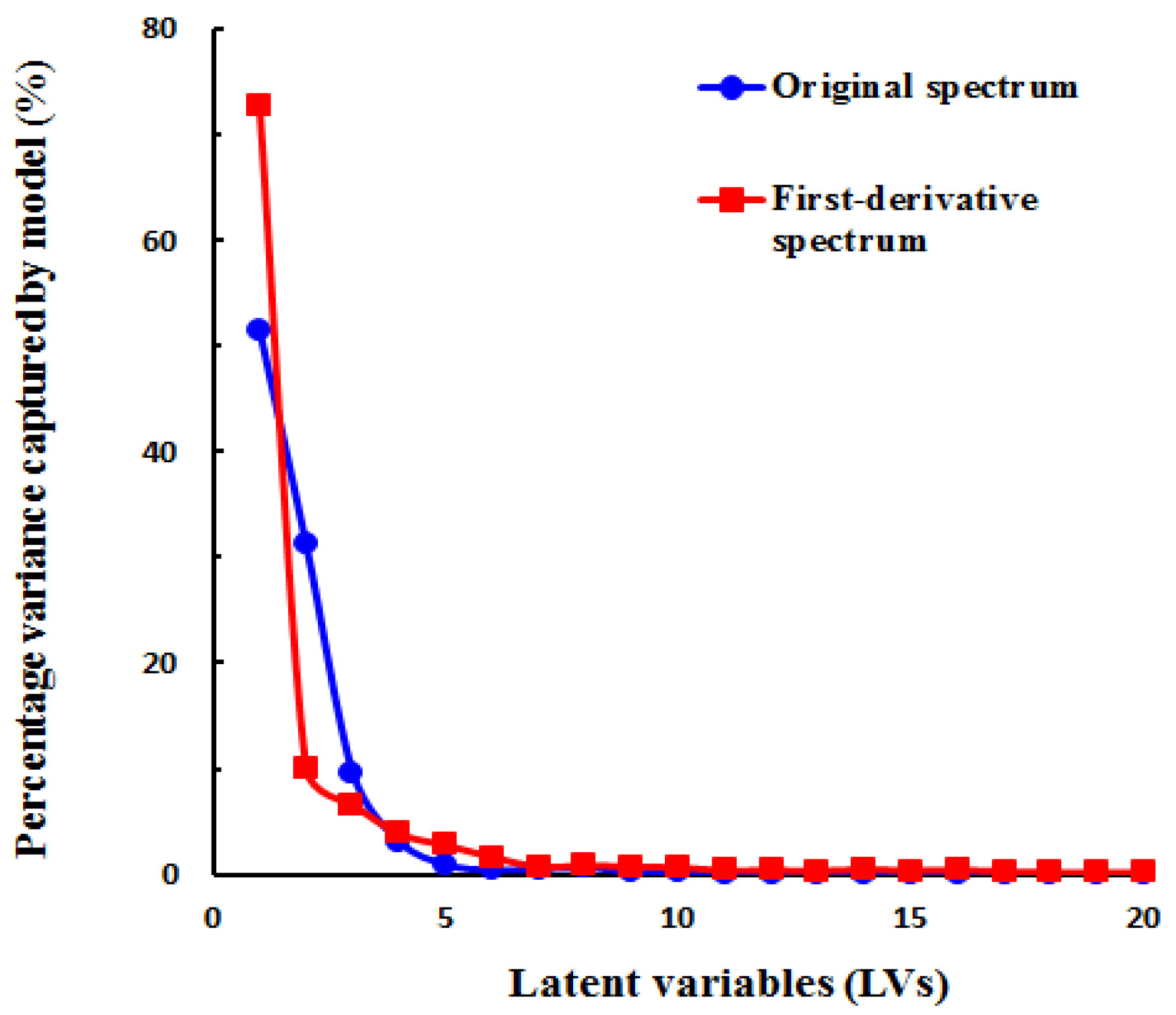[33] have found that the best wavelengths selected with SMLR might not be related to the absorption characteristics of the compounds of interest and do not produce consistent results between datasets. Hence, care should be taken when using SMLR to select wavelengths and estimate N concentration. Alternatively, the PLSR approach has been adopted to reduce the large number of measured collinear spectral variables to a few non-correlated latent variables (LVs), thereby avoiding the potential overfitting problems that are typically associated with SMLR [16,33].

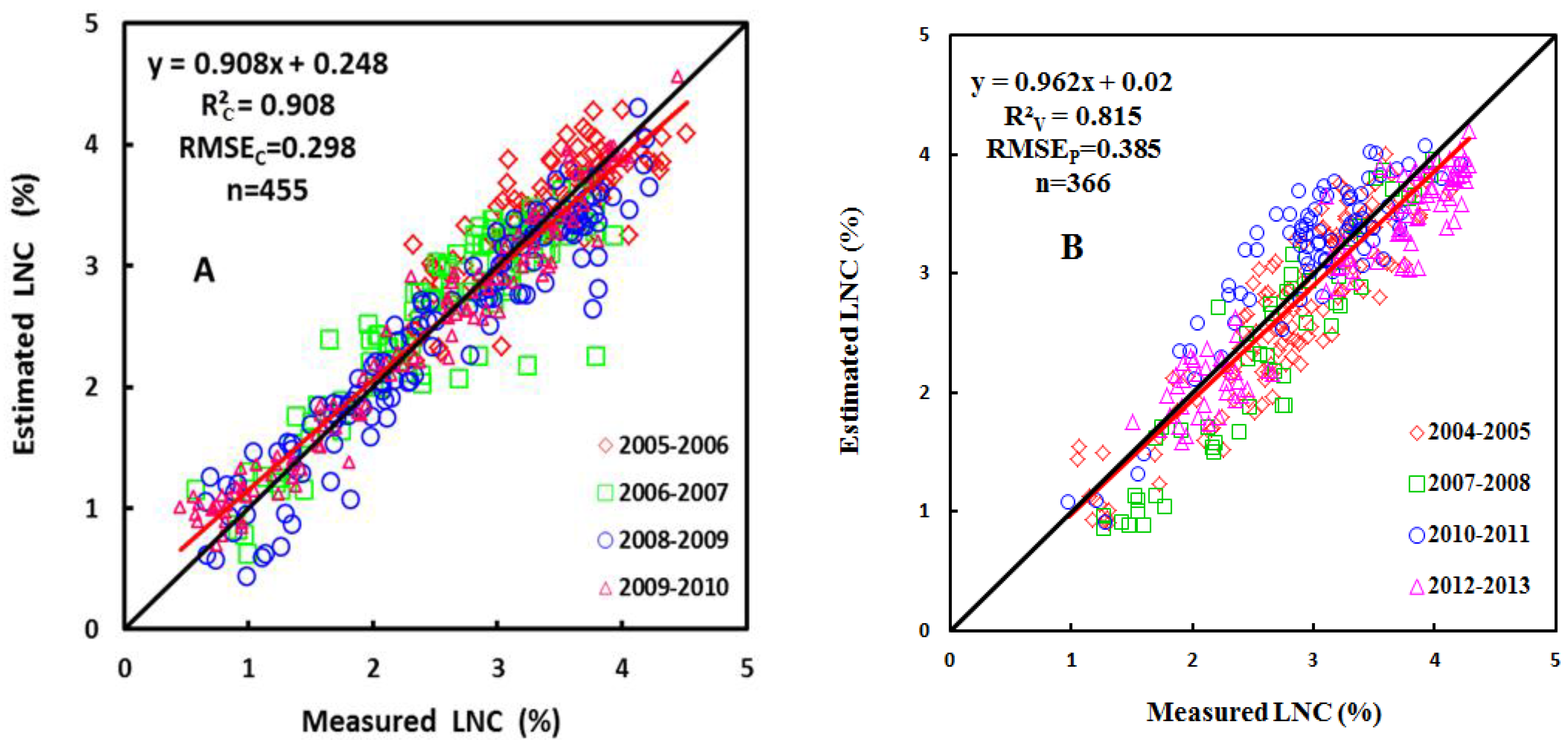
A number of spectrometric studies have been undertaken concerning the estimation of the N content of plants using CR, vegetation indices (VIs), SMLR and PLSR [8,10,11,12,16,33,34]. These approaches use an inconsistent number of wavelengths to estimate the N concentrations or estimate the chlorophyll status. Apart from these linear regression methods, some recent studies have investigated non-linear regression methods from the machine learning field such as artificial neural networks (ANNs) and support vector machines (SVMs) [34,35].

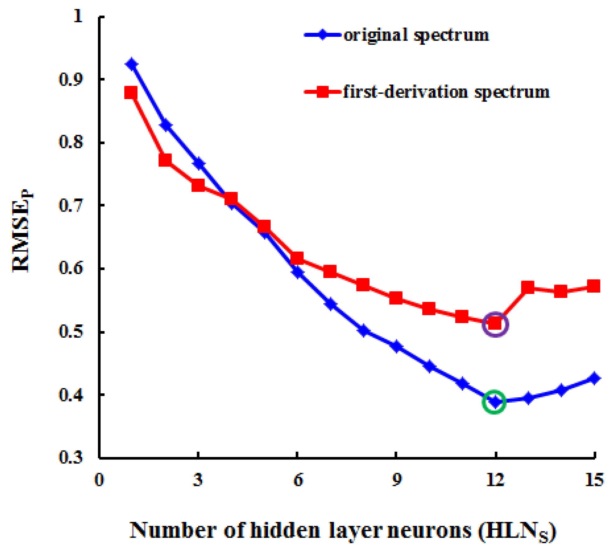
To date, the performance, advantages and disadvantages of leaf nitrogen concentration (LNC) estimation for wheat crops using ANN and SVM algorithms remain unclear. Currently, the ANN method is widely used in remote sensing to predict vegetation parameters and crop yields [6,34,35]. However, it inevitably suffers from the overfitting problem. Fortunately, some researchers reported the SVM method resolves the problem of overfitting encountered when analyzing high-dimensional data [36] and has been used to soil moisture [37], hourly typhoon rainfall [38], long-lead stream flows [39], leaf area index, and leaf chlorophyll density [40,41]. These studies have shown that the SVM approach is preferable to the ANN approach for these applications because of its greater generalizability. In addition to the conventional application, ANN and SVM methods should be assessed in a comparative way in terms of their performance and potential for the estimation of wheat LNC.

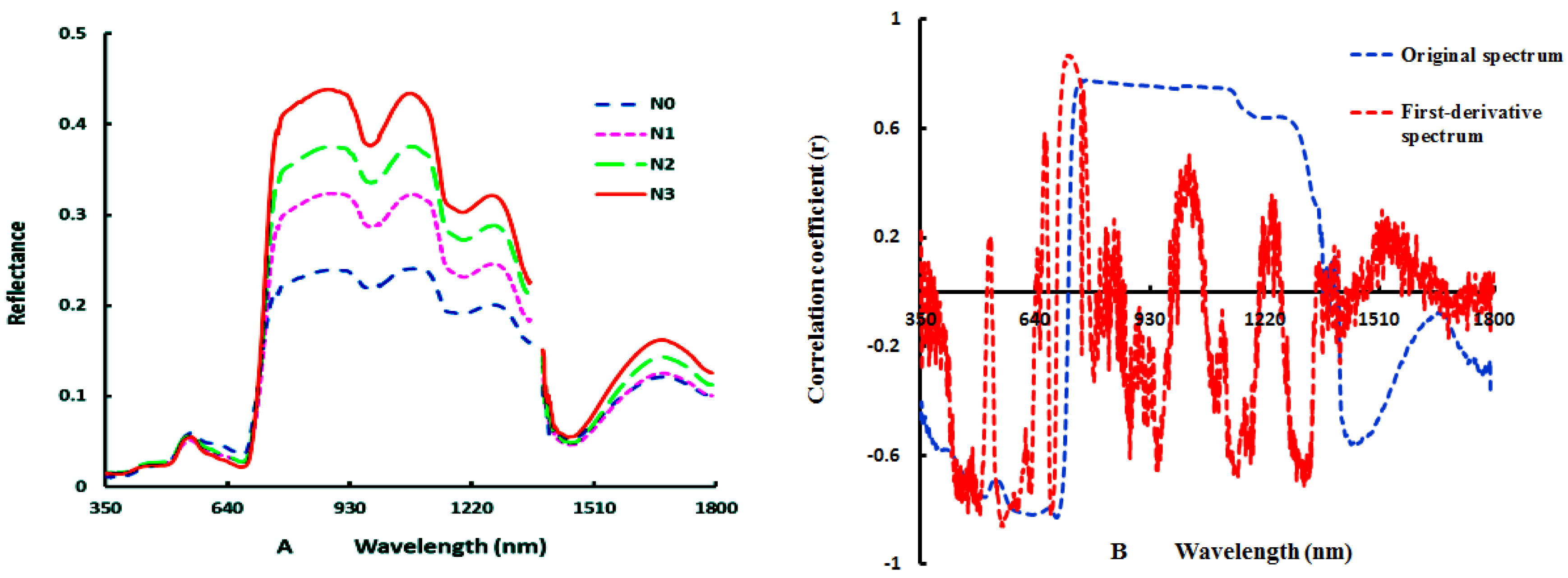
Currently, the first derivative is often used to decompose a mixed spectrum and reduce the noise in the hyperspectral region [41,42]. Mauser and Bach [43] have concluded that derivative spectral indices are very sensitive to LAI. Yoder and Pettigrew-Crosby [4] have found that first-order derivative spectra are the best predictors of the N and chlorophyll contents of big-leaf maples grown under different fertilization treatments. Johnson and Billow [44] have examined Douglas fir needles grown using various fertilization treatments and also found the first-order derivatives of the fresh leaf spectra to be strongly correlated with the total N concentration. Many studies have demonstrated the potential of derivative spectra for estimating chemical concentrations of non-crop vegetation types. However, few studies have examined the performance of first-order derivative spectra with respect to the LNC of fresh wheat crop leaves.

To the best of our knowledge, no studies in the literature have provided an evaluation of all these methods and their predictive equations for wheat LNC using a large number of samples accumulated over nine consecutive years of field trial experiments with a total of 821 wide representatively samples. Moreover, previous evaluations have focused on the prediction accuracies and have not reported results on computational efficiency and complex level, which may be a serious problem when using hyperspectral imaging data. To address these research gaps, this study presents the results of a comparative assessment of six retrieval methods applied to in situ measurements acquired over eight years for seven varieties, four eco-sites, and 821 samples. The main objectives were (1) to evaluate the ability and performance of various linear (CR, VIs, SMLR and PLSR) and nonlinear (ANN_S and SVM_S) regression methods based on the original and first derivative spectra for LNC estimation; and (2) to determine which method, input variable and model could estimate the LNC in winter wheat with higher accuracy, better robustness, less time, and less complexity.

2. Materials and Methods

2.1. Design of Field Experiments

Eight field experiments were conducted over eight growing seasons, with four located in Nanjing (32°03′N, 118°42′E), two in Rugao (32°15′N, 120°38′E), one in Hai’an (32°32′N, 120°28′E) and one in Yancheng (33°29′N, 120°28′E) in Jiangsu Province of eastern China. The experimental variables included different N fertilization rates and different cultivars of winter wheat. Each experiment consisted of a randomized complete block design with three replications. For all treatments, sufficient Ca(H₂PO₄)₂ and KCl were applied (150 kg·ha⁻¹) prior to seeding. Crop management followed local standard practices for wheat production. Additional details regarding the experimental design are provided in Table 1.

Table 1. Details of the eight field experiments.

Experi-ment(Exp.)	Year	Ecological Site	Wheat Cultivar	N Application Rates (kg·ha−1)	Sampling Dates	Number of Samples	Data Function
Exp. 1	04–05	Nanjing	Ningmai 9, Yangmai 12, Yumai 34	0, 75, 150, 225	19 March, 13/26 April, 3/6/12/24 May, 1 July	102	Validation
Exp. 2	05–06	Nanjing	Ningmai 9, Yumai 34 Yangmai 12	0, 75, 150, 225	19 March, 13/26 April, 3/6/12/24 May, 1 July	110	Calibration
Exp. 3	06–07	Yancheng	Yanmai 4110	0, 75, 150, 225 300	23 April, 17 May	103	Calibration
Exp. 4	07–08	Nanjing	Ningmai 9	90, 180, 270	8/23 April, 17 May	88	Validation
Exp. 5	08–09	Rugao	Yangmai 13	225, 275, 325	6/22 April, 6 May	120	Calibration
Exp. 6	09–10	Hai’an	Ningmai 13	0, 75, 150, 225	6/22 April, 6 May	122	Calibration
Exp. 7	10–11	Nanjing	Yangmai 18	150, 300	2/14/26 April, 5/17 May	93	Validation
Exp. 8	12–13	Rugao	Yangmai 18, Shengxuan 6	0, 100, 300	14/26 April, 3 May	83	Validation

Table 1. Details of the eight field experiments.

Experi-ment(Exp.)	Year	Ecological Site	Wheat Cultivar	N Application Rates (kg·ha−1)	Sampling Dates	Number of Samples	Data Function
Exp. 1	04–05	Nanjing	Ningmai 9, Yangmai 12, Yumai 34	0, 75, 150, 225	19 March, 13/26 April, 3/6/12/24 May, 1 July	102	Validation
Exp. 2	05–06	Nanjing	Ningmai 9, Yumai 34 Yangmai 12	0, 75, 150, 225	19 March, 13/26 April, 3/6/12/24 May, 1 July	110	Calibration
Exp. 3	06–07	Yancheng	Yanmai 4110	0, 75, 150, 225 300	23 April, 17 May	103	Calibration
Exp. 4	07–08	Nanjing	Ningmai 9	90, 180, 270	8/23 April, 17 May	88	Validation
Exp. 5	08–09	Rugao	Yangmai 13	225, 275, 325	6/22 April, 6 May	120	Calibration
Exp. 6	09–10	Hai’an	Ningmai 13	0, 75, 150, 225	6/22 April, 6 May	122	Calibration
Exp. 7	10–11	Nanjing	Yangmai 18	150, 300	2/14/26 April, 5/17 May	93	Validation
Exp. 8	12–13	Rugao	Yangmai 18, Shengxuan 6	0, 100, 300	14/26 April, 3 May	83	Validation

2.2. Measurements of Hyperspectral Reflectance

All canopy spectral measurements were performed using an ASD FieldSpec Pro FR2500 spectrometer (Analytical Spectral Devices, Boulder, CO, USA) [27]. This spectrometer was fitted with 25° field-of-view fiber optics operating in the 350–2500 nm spectral range with a sampling interval of 1.4 nm and spectral resolution of 3 nm between 350 and 1050 nm, and of 2 nm and 10 nm, respectively, between 1050 and 2500 nm. The spectrometer was equipped with three separate holographic diffraction gratings and three different detectors: VNIR (350–1000 nm), SWIR1 (1001–1800 nm), and SWIR2 (1801–2500 nm). Because the SWIR2 detector was influenced by water vapor in the field tests, the spectral response in the visible and near-infrared bands (350–1800 nm) was used to monitor the wheat LNC in this study. The measurements were conducted 1 m above the wheat canopy with a view diameter of 0.44 m under clear sky conditions between 10:00 a.m. and 2:00 p.m. (Beijing time). Measurements of vegetation irradiance were performed at five sample sites in each plot. Each sample consisted of an average of three scans at an optimized integration time. The resulting spectral file contained the continuous spectral reflectance data collected in 1 nm steps in the band region of 350–2500 nm. Panel irradiance measurements (two scans each) were performed before and after each vegetation measurement. The smoothing procedure of Savitzky and Golay [31], which uses a five-point moving window, was applied to preprocess the spectrum. After smoothing, the first derivative was calculated to eliminate background effects and reduce noise.

2.3. Determination of Leaf N Concentration

After each measurement of the canopy spectral reflectance, wheat plants from a 0.25 m² area (two 0.5 m rows) were collected from each plot to determine their LNC values (%). For each sample, all green leaves were separated from the stems, oven-dried at 70 °C to constant weight, and then weighed. The dried leaf samples were ground, passed through a 1 mm screen, and stored in plastic bags for subsequent chemical analysis. The total N concentration in the leaf tissues was determined using the micro-Kjeldahl method.

2.4. Data Analysis

In this study, six different algorithms (CR, SI, SMLR, PLSR, ANN, and SVM) were comparatively analyzed using MATLAB (2010b).

2.4.1. Continuum Removal (CR)

The CR method was first applied to isolate individual absorption features of interest [21]. Based on the N-absorption characteristics, a local starting point (550 nm) and ending point (750 nm) were selected for CR analysis in this study. The selected region is primarily influenced by chlorophyll absorption, represented by an exponential function [23] that is used for the retrieval of biochemical and biophysical parameters [15,22,23]. Three CR parameters were used: (1) the band depth (BD); (2) the band depth ratio (BDR) and (3) the normalized band depth index (NBDI) [23]. These three CR parameters were calculated using the methods of Curran [27] and Mutanga [23,45].

2.4.2. Vegetation Indices (VIs)

Three types of vegetation indices, including the normalized difference vegetation index (NDVI, (R_λ1 − R_λ2)/(R_λ1 + R_λ2)), ratio vegetation index (RVI, (R_λ1/R_λ2)), and soil-adjusted vegetation index (SAVI, [1.5 * (R_λ1 − R_λ2)/(R_λ1 + R_λ2 − 0.5)]), were calculated using the presented equations for all possible two-band combinations in the full spectral range. R_λ1 and R_λ2 represent those spectral reflectances drawn from the full spectral range.

2.4.3. Stepwise Multiple Linear Regression (SMLR)

SMLR was first proposed by Chatterjee and Price [46]. Using SMLR to filter the independent variables and construct regression models is a good approach to the current problem. With y as the independent variable and x as the dependent variable, the result is a linear relationship between the independent and dependent variables. Then, the multiple linear regression models take the following form:

$$\text{y}=b_0+b_1{x}_1+b_2{x}_2+\dots +b_k{x}_k+\mathrm{\epsilon }$$

(1)

where b₀ is a constant term, ε is a regression coefficient, and b₁, b₂, …, b_k are bands.

2.4.4. Partial Least-Squares Regression (PLSR)

The PLSR approach is a new type of multivariate statistical analysis algorithm that primarily considers a single dependent variable among the multiple variables of the regression model. In addition, PLSR is more effective under conditions in which the number of samples is fewer than the number of variables. Although the PLSR method is similar to principal component regression (PCR), PLSR actually involves decomposing both the spectra and the response variables simultaneously [47]. In this study, the spectral data were mean-centered before analysis, and the number of latent variables (LVs) was determined following the guidelines prescribed by Esbensen [48]. The optimal number of LVs was determined based on the relationship between the percentage variance captured by the model and the number of latent variables. With an increasing number of LVs, the percentage variance captured gradually changed, and the value indicated the optimal number of LVs. The basic PLSR methodology has been described in previous studies [46,49]. The objective of PLSR is to construct a linear model as follows:

$$Y=X\mathrm{\beta }+\mathrm{\epsilon }$$

(2)

where Y is a mean-centered vector of a dependent variable, X is a mean-centered matrix of the independent variables, β is a matrix of regression coefficients, and ε is a matrix of residuals.

2.4.5. Artificial Neural Networks (ANNs)

Multi-layer perceptron networks constitute one of the most widely used types of neural networks in the remote sensing community [50]. A typical ANN is composed of various layers (an input layer, an output layer, and several hidden layers), and each layer contains a number of interconnected nodes and activation functions [7]. In this study, the optimum number of hidden layer nodes (HLNs) was determined based on the minimum value of RMSE_P, and gradient descent with momentum was used to train the network using 5000 iterations.

2.4.6. Support Vector Machines (SVMs)

The SVM technique is a universal theory of machine learning originally developed by Vapnik and Cortes for pattern recognition and classification [51,52]. SVM regression models can map low-dimensional nonlinear input to high-dimensional linear output with good results. The SVM approach has many unique advantages in pattern recognition for small samples as well as nonlinear and high-dimensional cases. The kernel function is particularly important for SVM analysis. In this study, the sigmoid tanh kernel was used for SVM analysis, with the equation shown below (Equation (3)) [36]. The SVM parameters were selected based on the mean square error (MSE). The parameters with the lowest MSE in the SVM regression were considered the best.

$$K\left(x,y\right)=tanh\left(k\left(x,z\right)+v\right),k>0,v<0$$

(3)

where k is a scalar and v is a displacement parameter.

2.4.7. Calibration and Validation

Six algorithms (CR, SI, SMLR, PLSR, ANN, and SVM) using different numbers of wavelengths were applied to construct models for monitoring the wheat LNC. The data from Exp. 2, 3, 5, and 6 were used as the calibration set because they contained a wider range of representative data, including a higher number of samples of different cultivars, more ecological sites and more growth stages. Exp. 1, 4, 7, and 8 were used as the validation set (Table 2). The fitness was evaluated from a 1:1 plot of the predicted and observed data.

Table 2. The statistical parameters of the calibration and validation sets for the wheat leaf nitrogen content (LNC).

Dataset	Number of Samples	Names of Cultivars	Ecological Sites	Minimum (%)	Maximum (%)	Mean (%)	SD	CV
Calibration (Exp. 2, 3, 5, 6)	456	Ningmai 9, Yumai 34, Yangmai 12, Yanmai 4110, Yangmai 13, Ningmai 13	Nanjing, Yancheng, Rugao, Hai’an Nanjing, Rugao	0.45	4.52	2.66	0.98	0.37
Validation (Exp. 1, 4, 7, 8)	366	Ningmai 9, Yangmai 12, Yumai 34,Yangmai 18, Shengxuan 6		0.98	4.29	2.92	0.77	0.26
All data	822	All of the above		0.45	4.52	2.78	0.87	0.32

Table 2. The statistical parameters of the calibration and validation sets for the wheat leaf nitrogen content (LNC).

Dataset	Number of Samples	Names of Cultivars	Ecological Sites	Minimum (%)	Maximum (%)	Mean (%)	SD	CV
Calibration (Exp. 2, 3, 5, 6)	456	Ningmai 9, Yumai 34, Yangmai 12, Yanmai 4110, Yangmai 13, Ningmai 13	Nanjing, Yancheng, Rugao, Hai’an Nanjing, Rugao	0.45	4.52	2.66	0.98	0.37
Validation (Exp. 1, 4, 7, 8)	366	Ningmai 9, Yangmai 12, Yumai 34,Yangmai 18, Shengxuan 6		0.98	4.29	2.92	0.77	0.26
All data	822	All of the above		0.45	4.52	2.78	0.87	0.32

The performances of all models were evaluated based on several statistical parameters, including the calibration R² (R²_C), the root mean square error of calibration (RMSE_C; see Equation (4)), validation R² (R²_V), and the root mean square error of prediction (RMSE_P). All calculations were performed using custom-written MATLAB (2010b) scripts. Higher values of R²_C, R²_V, and PDP and lower values of RMSE_C and RMSE_P indicated higher precision and accuracy of the model. The running time was calculated using MATLAB 10b, and the level of operating complexity was determined based on the algorithm used to construct the model and the number of wavelengths.

$$RMS{E}_c=\sqrt{{\displaystyle \sum }_{i=1}^n{\left(Y_{est,i}-Y_{mea,i}\right)}^2/n}$$

(4)

where Y_est,i is the estimated LNC_i, Y_mea,i is the measured LNC_i, and n is the number of samples. RMSE_P was also calculated using Equation (4).

The ratio of prediction to deviation (RPD) was calculated as follows:

$$RPD=\frac{SD}{RMS{E}_P}$$

(5)

where SD is the standard deviation. A value of RPD > 2.0 indicates a stable and accurate predictive model, an RPD value between 1.4 and 2.0 indicates a fair model that could be improved by more accurate prediction techniques, and a value of RPD < 1.4 indicates poor predictive capacity [53].

3. Results

3.1. Changes in the Canopy Spectral Reflectance and Its Relationship with the LNC for Wheat

The Yumai 34 cultivar at the various N rates used in Experiment 3 is used as an example of the analysis of the spectral variations in Figure 1A. The results show that the reflectance decreases in the visible region with increasing N concentration because of the increased absorption of the pigments and increases in the near-infrared region because of the effects of moisture and leaf structure. Further analysis of the relationships between the LNC and the reflectance determined from the original and first derivative canopy spectra was also performed (Figure 1B). A negative correlation was found in the visible region (350–710 nm) for the original spectra, whereas a positive correlation was observed in the near-infrared range (710–1410 nm), which was regarded as a higher reflectance platform (R² > 0.78, between 760 and 1100 nm). The first derivative canopy spectrum exhibited a strong correlation throughout a wavelength range that was similar to that of the original canopy spectrum but contained more prominent peaks.

Figure 1. (A) Canopy spectral reflectance under four N rates at booting for Yumai 34 in Experiment 3; (B) Correlation of the LNC with the original and first derivative spectra.

Figure 1. (A) Canopy spectral reflectance under four N rates at booting for Yumai 34 in Experiment 3; (B) Correlation of the LNC with the original and first derivative spectra.

3.2. Models for Estimating the LNC Based on Six Algorithms Using Different Numbers of Wavelengths

3.2.1. CR with One Wavelength

Figure 2A displays the original canopy spectrum, continuum line, and CR spectrum of Yumai 34 in the booting stage at an N rate of 150 kg/ha in Experiment 3. Figure 2B shows the correlation coefficients between the BD, BDR, and NBDI and the canopy LNC of the wheat. We found that the correlation coefficient between the BD and the canopy LNC exhibited a less distinct variation and that the correlation coefficients between the BDR and NBDI and the canopy LNC exhibited their lowest values between 550 and 750 nm. Figure 2B indicates that BD₇₀₉, BDR₇₁₃, and NBDI₇₂₇ showed the highest correlations.

Table 3 shows the values of the BDR, BD, and NBDI along with those of R²_C, RMSE_C, R²_V, RMSE_P, and RDP for the LNC model. The three CR parameters indicate a good slope value for the 1:1 line and also require little running time. Among the three indices, BD₇₀₉ was the most effective parameter because it yielded not only the highest precision on the calibration set but also had the highest accuracy on the validation set. NBDI₇₂₇ was the least effective parameter because of its poor stability. Figure 3 shows a scatter diagram of the LNC values from the model obtained using BD₇₀₉ from the original canopy spectra.

Figure 2. (A) The original spectrum, continuum line, and continuum-removed spectrum of Yumai 34 at the booting stage at an N rate of 150 kg/ha in Experiment 3. (B) Correlation coefficients between the band depth (BD), the band depth ratio (BDR), and the normalized band depth index (NBDI) and the LNC in the range of 550–750 nm.

Figure 2. (A) The original spectrum, continuum line, and continuum-removed spectrum of Yumai 34 at the booting stage at an N rate of 150 kg/ha in Experiment 3. (B) Correlation coefficients between the band depth (BD), the band depth ratio (BDR), and the normalized band depth index (NBDI) and the LNC in the range of 550–750 nm.

Table 3. The best-performing LNC models based on the continuum removal (CR) parameters for the calibration and validation sets.

Band Range	Input Parameter	Calibration			Validation
		Equation	R2C	RMSEC	R2V	RMSEP	RPD	CE (min)	CL
550–750	BD709	y = 0.823 × e2.056x	0.78	0.46	0.78	0.42	1.84	0.07 min	Low
	BDR713	y = 0.536 × e2.588x	0.78	0.48	0.74	0.45	1.72	0.08 min	Low
	NBDI727	y = 9.147 × e2.51x	0.76	0.54	0.71	0.49	1.56	0.07 min	Low

Notes: BD: band depth; BDR, band depth ratio; NBDI: normalized band depth index.

Table 3. The best-performing LNC models based on the continuum removal (CR) parameters for the calibration and validation sets.

Band Range	Input Parameter	Calibration			Validation
		Equation	R2C	RMSEC	R2V	RMSEP	RPD	CE (min)	CL
550–750	BD709	y = 0.823 × e2.056x	0.78	0.46	0.78	0.42	1.84	0.07 min	Low
	BDR713	y = 0.536 × e2.588x	0.78	0.48	0.74	0.45	1.72	0.08 min	Low
	NBDI727	y = 9.147 × e2.51x	0.76	0.54	0.71	0.49	1.56	0.07 min	Low

Notes: BD: band depth; BDR, band depth ratio; NBDI: normalized band depth index.

Figure 3. Calibration (A) and validation (B) of the model based on BD₇₀₉ from the original canopy spectra.

Figure 3. Calibration (A) and validation (B) of the model based on BD₇₀₉ from the original canopy spectra.

3.2.2. VI with Two Wavelengths

Figure 4 shows the coefficients of determination (R²) of the linear regressions between the LNC and the NDVI, RVI, and SAVI constructed from arbitrary two-band combinations based on the original and first derivative canopy spectra. The maximum R²_C values for the NDVI, RVI, and SAVI based on the original canopy spectra were 0.830, 0.828, and 0.844, respectively, and those based on the first derivative canopy spectra were 0.858, 0.864, and 0.851, respectively. For the original spectra, the strongest correlation (R² > 0.75) between the arbitrary two-band combinations and the wheat LNC was found in the visible and near-infrared ranges. For the first derivative canopy spectra, the best band combination (R² > 0.75) was in the visible range. In the contour maps of the coefficient of determination (R² > 0.5), more regions were identified based on the original canopy spectra than were identified based on the first derivative canopy spectra.

Figure 4. Contour maps of the coefficients of determination (R² > 0.5) between the normalized difference vegetation index (NDVI), ratio vegetation index (RVI), and soil-adjusted vegetation index (SAVI) and the canopy LNC based on the original and first derivative canopy spectra.

Figure 4. Contour maps of the coefficients of determination (R² > 0.5) between the normalized difference vegetation index (NDVI), ratio vegetation index (RVI), and soil-adjusted vegetation index (SAVI) and the canopy LNC based on the original and first derivative canopy spectra.

Based on the statistical parameters of R²_C, RMSE_C, R²_V, RMSE_P, and RDP for the calibration and validation sets and the spectrum principle, we selected the optimal wavelength and spectral index (Table 4). Table 4 shows that three types of VI_S yielded better precision for the first derivative canopy spectra than for the original canopy spectra in the calibration set. The optimal wavelengths selected based on the NDVI, RVI, and SAVI were very similar. For the original spectra, the performance of SAVI(R₁₂₀₀, R₇₀₅) was significantly better than that of NDVI(R₁₃₄₀, R₇₀₀), which was very similar to that of RVI(R₇₀₀, R₁₃₃₅). For the first derivative canopy spectra, the optimal wavelength combinations were observed between 695 and 700 nm in the visible range. According to a comprehensive evaluation of the calibration and validation performance, the SAVI obtained using the original canopy spectra performed best and exhibited good stability. In particular, the adjustable index L(L = 0.5) for the SAVI yielded superior results for the reduction of soil noise. Figure 5 shows a scatter diagram of SAVI(R₁₂₀₀, R₇₀₅) and the validation performance on the original canopy spectra.

Table 4. The best-performing LNC models based on the vegetation indices (VIs) for the calibration and validation sets.

VI	λ1 (nm)	λ2 (nm)	Calibration			Validation
			Equation	R2C	RMSEC	R2V	RMSEP	RPD	CE (min)	CL
NDVI	1340	700	y = 5.58x − 0.02	0.83	0.39	0.76	0.41	1.86	0.11	Low
RVI	700	1335	y = −5.63x + 4.69	0.83	0.39	0.76	0.40	1.95	0.10	Low
SAVI	1200	705	y = 8.72x + 0.10	0.84	0.38	0.80	0.38	2.01	0.10	Low
NDVI *	710	690	y = 3.59x + 1.38	0.86	0.36	0.72	0.51	1.53	0.11	Low
RVI *	700	695	y = 3.19x − 1.38	0.86	0.36	0.68	0.57	1.35	0.11	Low
SAVI *	710	695	y = 283.2x + 1.8	0.85	0.37	0.76	0.40	1.92	0.10	Low

Note: * vegetation indices calculated with the first derivatives of reflectance spectra.

Table 4. The best-performing LNC models based on the vegetation indices (VIs) for the calibration and validation sets.

VI	λ1 (nm)	λ2 (nm)	Calibration			Validation
			Equation	R2C	RMSEC	R2V	RMSEP	RPD	CE (min)	CL
NDVI	1340	700	y = 5.58x − 0.02	0.83	0.39	0.76	0.41	1.86	0.11	Low
RVI	700	1335	y = −5.63x + 4.69	0.83	0.39	0.76	0.40	1.95	0.10	Low
SAVI	1200	705	y = 8.72x + 0.10	0.84	0.38	0.80	0.38	2.01	0.10	Low
NDVI *	710	690	y = 3.59x + 1.38	0.86	0.36	0.72	0.51	1.53	0.11	Low
RVI *	700	695	y = 3.19x − 1.38	0.86	0.36	0.68	0.57	1.35	0.11	Low
SAVI *	710	695	y = 283.2x + 1.8	0.85	0.37	0.76	0.40	1.92	0.10	Low

Note: * vegetation indices calculated with the first derivatives of reflectance spectra.

Figure 5. The relationship between SAVI(R₁₂₀₀, R₇₀₅) and the wheat LNC (A); and the 1:1 relationship between the measured LNC and those estimated values based on SAVI(R₁₂₀₀, R₇₀₅) (B).

Figure 5. The relationship between SAVI(R₁₂₀₀, R₇₀₅) and the wheat LNC (A); and the 1:1 relationship between the measured LNC and those estimated values based on SAVI(R₁₂₀₀, R₇₀₅) (B).

3.2.3. SMLR with Multiple Wavelengths

The wavelengths selected by SMLR were 384, 492, 695, 1339, and 1369 nm for the original canopy spectra and 508, 681, 722, 960, and 1264 nm for the first derivative canopy spectra. The R²_C values for the SMLR-OS and SMLR-FDS models were 0.869 and 0.855, respectively. The values of the statistical parameters for calibration and validation (R²_C, RMSE_C, R²_V, RMSE_P, and RDP) and the wavelengths selected are summarized in Table 5. The results show that SMLR based on the original canopy spectra offered a higher accuracy in the monitoring of the wheat LNC (R²_C = 0.869, RMSE_C = 0.353, R²_V = 0.778, RMSE_P = 0.390, RDP = 1.974); however, no significant difference was observed between the SMLR-OS and SMLR-FDS models. These two models could be expressed as follows:

• SMLR-OS model:

  y = 1.941 − 92.315 * b₃₈₄ + 122.732 * b₄₉₂ − 55.338 * b₆₉₅ + 8.591 * b₁₃₃₉ − 0.321 * b₁₃₆₉

  (6)
• SMLR-FDS model:

  y = 2.189 − 980.699 * b_FD508 − 1034.799 * b_FD681 + 303.223 * b_FD722 + 195.538 * b_FD960 + 451.419 * b_FD1264

  (7)

where b and b_FD represent the reflectance of the original and first derivative wavelength spectra, e.g., b₆₉₅ is the reflectance at 695 nm and b_FD722 is the first derivative reflectance at 722 nm.

Table 5. The best-performing LNC models based on stepwise multiple linear regressions (SMLR) for the calibration and validation sets.

Model	Selected Wavelengths (nm)	Calibration		Validation
		R2c	RMSEC	R2v	RMSEP	RDP	CE (min)	CL
SMLR-OS	695, 1339, 492, 384, 1369	0.87	0.35	0.78	0.39	1.97	32.15	Middle
SMLR-FDS	722, 681, 1264, 508, 960	0.86	0.37	0.76	0.39	1.95	33.16	Middle

Notes: OS: original canopy spectra; FDS: first derivative canopy spectra.

Table 5. The best-performing LNC models based on stepwise multiple linear regressions (SMLR) for the calibration and validation sets.

Model	Selected Wavelengths (nm)	Calibration		Validation
		R2c	RMSEC	R2v	RMSEP	RDP	CE (min)	CL
SMLR-OS	695, 1339, 492, 384, 1369	0.87	0.35	0.78	0.39	1.97	32.15	Middle
SMLR-FDS	722, 681, 1264, 508, 960	0.86	0.37	0.76	0.39	1.95	33.16	Middle

Notes: OS: original canopy spectra; FDS: first derivative canopy spectra.

3.2.4. PLSR with All Wavelengths

Figure 6 shows the changes in the percentage variance captured with an increasing number of latent variables (LVs) using the original and first derivative canopy spectra. When the number of latent variables (LVs) was greater than five or seven for the original or first derivative spectra, respectively, the percentage variance captured by the model decreased only minimally. Therefore, we selected five and seven latent variables (LVs) for the PLSR analyses based on the original and first derivative canopy spectra, respectively.

Figure 6. Changes in the variance explained by the latent variables (LVs) based on the original and first derivative canopy spectra.

Figure 6. Changes in the variance explained by the latent variables (LVs) based on the original and first derivative canopy spectra.

The results of the PLSR analyses are shown in Table 6. With all wavelengths used as input variables, the PLSR analysis based on the first derivative canopy spectra (FDS) demonstrated a higher estimation accuracy for the canopy LNC than did the analysis based on the original canopy spectra for both the calibration and validation sets, with statistical parameters of R²_C = 0.908, RMSE_C = 0.298, R²_V = 0.815, RMSE_P = 0.385, and RDP = 2.000. Figure 7 shows the results of predicting the LNC for winter wheat based on the calibration and validation sets using the PLSR-FDS model.

Table 6. The best-performing LNC models based on partial least-squares regression (PLSR) for the calibration and validation sets.

Model	Input Variables	Calibration			Validation
		LVs	R2c	RMSEC	R2v	RMSEP	RDP	CE (min)	CL
PLSR-OS	all wavelengths	5	0.85	0.37	0.81	0.35	2.22	6.10	High
PLSR-FDS	all wavelengths	7	0.91	0.30	0.815	0.39	2.00	5.50	High

Notes: OS: original canopy spectra; FDS: first derivative canopy spectra.

Table 6. The best-performing LNC models based on partial least-squares regression (PLSR) for the calibration and validation sets.

Model	Input Variables	Calibration			Validation
		LVs	R2c	RMSEC	R2v	RMSEP	RDP	CE (min)	CL
PLSR-OS	all wavelengths	5	0.85	0.37	0.81	0.35	2.22	6.10	High
PLSR-FDS	all wavelengths	7	0.91	0.30	0.815	0.39	2.00	5.50	High

Notes: OS: original canopy spectra; FDS: first derivative canopy spectra.

Figure 7. The 1:1 relationship between the measured LNC and those estimated values using the PLSR analysis on the first derivative canopy spectra (PLSR-FDS) model for the calibration (A) and validation (B) sets.

Figure 7. The 1:1 relationship between the measured LNC and those estimated values using the PLSR analysis on the first derivative canopy spectra (PLSR-FDS) model for the calibration (A) and validation (B) sets.

3.2.5. ANN with All Wavelengths

Figure 8 shows the changes in RMSE_P as a function of the number of hidden layer neurons (HLNs). The results indicate that the value of RMSE_P is lowest when the number of hidden neurons is equal to twelve. Therefore, we selected 12 as the optimal number of HLNs for the ANN analyses based on the original and first derivative canopy spectra.

Table 7 shows the results of the ANN-based LNC models for both the calibration and validation sets. According to Table 7, when all wavelengths were used as input variables for the ANN analysis, the ANN-FDS model offered a higher estimation accuracy for LNC monitoring than did the ANN-OS model for the calibration set. However, for the validation set, the ANN-OS model exhibited higher estimation accuracy than the ANN-FDS model and the slope value for the ANN-OS model was closer to 1 than that for the ANN-FDS model. Overall, the model based on all wavelengths in the first derivative canopy spectra yielded the higher estimation accuracy for the calibration set (R²_C = 0.987, RMSE_C = 0.111), but for the validation set, it exhibited the lower estimation accuracy (R²_V = 0.734, RMSE_P = 0.512, RDP = 1.504). The difference in performance between the calibration and validation sets indicates that the ANN method appears to suffer from overfitting when many input variables are used.

Figure 8. Changes in RMSE_P as a function of the number of hidden layer neurons (HLNs) for the original and first derivative canopy spectra.

Figure 8. Changes in RMSE_P as a function of the number of hidden layer neurons (HLNs) for the original and first derivative canopy spectra.

Table 7. The best-performing artificial neural networks (ANNs) -based LNC models for the calibration and validation sets.

Inputs	Optimal Numbers of Neurons			Calibration		Validation
	Input	Hidden	Output	R2C	RMSEC	R2V	RMSEP	RDP	CE (min)	CL
ANN-OS	1451	12	1	0.95	0.22	0.76	0.45	1.72	71.50	High
ANN-FDS	1451	12	1	0.99	0.18	0.73	0.51	1.50	67.20	High
ANN-PCA-OS	9	4	1	0.94	0.25	0.796	0.35	1.44	15.60	High
ANN-PCA-FDS	11	5	1	0.95	0.22	0.72	0.41	1.48	14.80	High

Note: OS: original canopy spectra; FDS: first derivative canopy spectra; ANN-PCA-OS indicates that we used PCA to select the primary factor and then used the PCA-derived factor to execute the ANN model.

Table 7. The best-performing artificial neural networks (ANNs) -based LNC models for the calibration and validation sets.

Inputs	Optimal Numbers of Neurons			Calibration		Validation
	Input	Hidden	Output	R2C	RMSEC	R2V	RMSEP	RDP	CE (min)	CL
ANN-OS	1451	12	1	0.95	0.22	0.76	0.45	1.72	71.50	High
ANN-FDS	1451	12	1	0.99	0.18	0.73	0.51	1.50	67.20	High
ANN-PCA-OS	9	4	1	0.94	0.25	0.796	0.35	1.44	15.60	High
ANN-PCA-FDS	11	5	1	0.95	0.22	0.72	0.41	1.48	14.80	High

Note: OS: original canopy spectra; FDS: first derivative canopy spectra; ANN-PCA-OS indicates that we used PCA to select the primary factor and then used the PCA-derived factor to execute the ANN model.

3.2.6. SVM with All Wavelengths

Table 8 summarizes the performance of the SVM-based LNC models with different input variables. The results show that the SVM-based models using all wavelengths in the first derivative spectra demonstrated better performance on the calibration set; however, the SVM-OS model offered slightly better performance on the validation set, with slightly higher R²V and RDP values and a shorter running time. Figure 9 shows the 1:1 relationship between the measured LNC and those estimated using the SVM-FDS model for the calibration and validation sets.

Table 8. The best-performing support vector machines (SVMs)-based LNC models for the calibration and validation sets.

Model	Input Variables	Calibration		Validation
		R2C	RMSEC	R2V	RMSEV	RDP	CE (min)	CL
SVM-OS	All wavelengths	0.96	0.21	0.80	0.38	2.05	20.34	High
SVM-FDS	All wavelengths	0.96	0.19	0.78	0.37	2.02	21.17	High
ANN-PCA-OS	9PCA	0.94	0.20	0.67	0.47	1.64	5.64	High
ANN-PCA-FDS	11PCA	0.92	0.27	0.55	0.57	1.36	5.76	High

Notes: OS, original canopy spectra; FDS, first derivative canopy spectra.

Table 8. The best-performing support vector machines (SVMs)-based LNC models for the calibration and validation sets.

Model	Input Variables	Calibration		Validation
		R2C	RMSEC	R2V	RMSEV	RDP	CE (min)	CL
SVM-OS	All wavelengths	0.96	0.21	0.80	0.38	2.05	20.34	High
SVM-FDS	All wavelengths	0.96	0.19	0.78	0.37	2.02	21.17	High
ANN-PCA-OS	9PCA	0.94	0.20	0.67	0.47	1.64	5.64	High
ANN-PCA-FDS	11PCA	0.92	0.27	0.55	0.57	1.36	5.76	High

Notes: OS, original canopy spectra; FDS, first derivative canopy spectra.

Figure 9. The 1:1 relationship between the measured LNC and those estimated using the SVM-FDS model for the calibration (A) and validation (B) sets.

Figure 9. The 1:1 relationship between the measured LNC and those estimated using the SVM-FDS model for the calibration (A) and validation (B) sets.

3.3. Evaluation and Comparison of the Robustness of the Six Algorithms

We compared the robustness of the six algorithms based on the statistical parameters R²_C, RMSE_C, R²_V, RMSE_P, CE and CL (Table 9). The results show that with an increasing number of wavelengths, the value of R²_C increased from 0.78 for BD₇₀₉ to 0.96 for SVM-FDS. However, the value of R²_V did not exhibit a similar increase. The CR algorithms used only one wavelength and demonstrated the poorest performance on both the calibration and validation sets, although they also required less running time and had lower complexity. The SAVI(R₁₂₀₀, R₇₀₅) method required only two wavelengths and offered better performance on both the calibration and validation sets (R²_C = 0.844, RMSE_C = 0.384, R²_V = 0.795, RMSE_P = 0.384, RDP = 2.005, and running time = 0.10 min). The SMLR-OS method used five wavelengths, whereas the PLSR-FDS, ANN-OS and SVM-FDS methods used all available wavelengths. Although PLSR-FDS demonstrated the best R²_V performance on the validation set, with a value of 0.82, the errors in calibration and validation sets were higher than those for SVM-FDS. Therefore, the SVM-based method yielded a higher prediction accuracy than the other methods on the calibration set (R²_C = 0.961, RMSE_C = 0.193, R²_V = 0.776, RMSE_P = 0.382, RDP = 2.016, and running time = 21.17 min). In addition, we found that with an increasing number of wavelengths, the running time increased; the BD₇₀₉ method exhibited the shortest running time (0.07 min), whereas the ANN-OS method required the longest running time (71.50 min), and the operational complexity also correspondingly increased. With regard to the slope of the 1:1 line, the SMLR-OS method yielded the smallest slope value, whereas the BD₇₀₉ method produced the greatest slope value. The SVM-FDS and SAVI(R₁₂₀₀, R₇₀₅) methods offered higher accuracy. However, SVM-FDS incurred a higher cost, as reflected in its use of multiple wavelengths, its higher complexity level, and its longer running time.

Table 9. The robustness evaluation of the wheat LNC models based on the six considered algorithms.

Method	Wavelengths (nm)	Calibration		Validation
		R2C	RMSEC	R2V	RMSEP	RDP	CE (min)	CL
BD709	709	0.78	0.46	0.78	0.42	1.84	0.07	Low
SAVI(R1200, R705)	1200, 705	0.84	0.38	0.80	0.38	2.01	0.10	Low
SMLR-OS	695, 1339,492,384,1369	0.87	0.35	0.78	0.39	1.97	33.16	Middle
PLSR-FDS	All wavelengths	0.91	0.30	0.82	0.39	2.00	5.50	High
ANN-OS	All wavelengths	0.95	0.22	0.76	0.45	1.72	71.50	High
SVM-FDS	All wavelengths	0.96	0.19	0.78	0.37	2.02	21.17	High

Table 9. The robustness evaluation of the wheat LNC models based on the six considered algorithms.

Method	Wavelengths (nm)	Calibration		Validation
		R2C	RMSEC	R2V	RMSEP	RDP	CE (min)	CL
BD709	709	0.78	0.46	0.78	0.42	1.84	0.07	Low
SAVI(R1200, R705)	1200, 705	0.84	0.38	0.80	0.38	2.01	0.10	Low
SMLR-OS	695, 1339,492,384,1369	0.87	0.35	0.78	0.39	1.97	33.16	Middle
PLSR-FDS	All wavelengths	0.91	0.30	0.82	0.39	2.00	5.50	High
ANN-OS	All wavelengths	0.95	0.22	0.76	0.45	1.72	71.50	High
SVM-FDS	All wavelengths	0.96	0.19	0.78	0.37	2.02	21.17	High

We further categorized the samples using three grouping variables (variety, ecological site, and growth stage) to compare the robustness of the optimal LNC model algorithms (Table 10). The results show that the prediction accuracy was always improved with an increasing number of wavelengths for each of the three grouping variables. However, the CE and CL also substantially increased. The results also show that the six algorithms were suitable and robust for the Ningmai 9 and Shengxuan 6 varieties, with maximum R²_V values of 0.86 and 0.88, respectively, and that the SVM-FDS algorithm offered the best overall performance, with a mean R²_V value of 0.79 for all five varieties. However, a suitable algorithm could not be found for the Yangmai 12 and Yumai 34 varieties, for which the R²_V values ranged from 0.65 to 0.80. These results demonstrate that the Ningmai 9 variety represents a generally adaptable variety and that the SVM-FDS method may be better suited than the other methods to cope with potential confounding factors for most varieties. Of the two ecological-site-based groups, Rugao yielded better results than did Nanjing for all six algorithms, with R²_V values ranging from 0.80 to 0.90. The robustness of the PLSR-FDS and SVM-FDS methods was particularly strong; these methods were suitable for both ecological sites, with R²_V values of 0.85 and 0.84, respectively. For the two growth-stage-based groups, the six algorithms all yielded better and more stable results for the stage of heading and anthesis, with R²_V values ranging from 0.78 to 0.86. The statistical parameters indicated poorer performance in the stage of jointing and booting.

Table 10. Robustness of the LNC models based on the six algorithms when the samples are categorized using three grouping variables (variety, ecological site, and growth stage).

Grouping Variable	Algorithm	Sub-Group	Validation				R2V–RMSEP
			R2V	RMSEP	CE (min)	CL
Variety	BD709	Ningmai 9	0.84	0.37	0.07	Low	0.47
		Yangmai 12	0.73	0.38	0.07	Low	0.36
		Yumai 34	0.80	0.28	0.07	Low	0.52
		Yangmai 18	0.71	0.48	0.07	Low	0.23
		Shengxuan 6	0.76	0.43	0.07	Low	0.33
	SAVI(R1200, R705)	Ningmai 9	0.80	0.43	0.10	Low	0.37
		Yangmai 12	0.75	0.41	0.10	Low	0.34
		Yumai 34	0.75	0.36	0.10	Low	0.40
		Yangmai 18	0.86	0.31	0.10	Low	0.55
		Shengxuan 6	0.77	0.36	0.10	Low	0.41
	SMLR-OS	Ningmai 9	0.83	0.47	16.23	Middle	0.36
		Yangmai 12	0.67	0.40	15.21	Middle	0.27
		Yumai 34	0.67	0.35	17.32	Middle	0.32
		Yangmai 18	0.81	0.36	16.46	Middle	0.45
		Shengxuan 6	0.77	0.38	15.35	Middle	0.39
	PLSR-FDS	Ningmai 9	0.86	0.38	5.21	High	0.48
		Yangmai 12	0.76	0.34	5.74	High	0.42
		Yumai 34	0.67	0.32	5.32	High	0.35
		Yangmai 18	0.81	0.36	5.21	High	0.45
		Shengxuan 6	0.88	0.35	5.56	High	0.53
	ANN-OS	Ningmai 9	0.85	0.44	65.23	High	0.41
		Yangmai 12	0.78	0.44	64.32	High	0.34
		Yumai 34	0.65	0.36	65.45	High	0.30
		Yangmai 18	0.76	0.42	63.23	High	0.34
		Shengxuan 6	0.77	0.55	62.89	High	0.22
	SVM-FDS	Ningmai 9	0.84	0.40	19.21	High	0.44
		Yangmai 12	0.79	0.36	18.32	High	0.43
		Yumai 34	0.67	0.42	18.21	High	0.25
		Yangmai 18	0.79	0.36	19.72	High	0.43
		Shengxuan 6	0.87	0.35	19.32	High	0.52
Ecological site	BD709	Nanjing	0.76	0.42	0.08	Low	0.34
		Rugao	0.80	0.41	0.08	Low	0.39
	SAVI(R1200, R705)	Nanjing	0.78	0.40	0.11	Low	0.38
		Rugao	0.85	0.34	0.11	Low	0.51
	SMLR-OS	Nanjing	0.77	0.42	28.22	Middle	0.35
		Rugao	0.86	0.37	12.32	Middle	0.49
	PLSR-FDS	Nanjing	0.80	0.38	5.86	High	0.42
		Rugao	0.90	0.31	5.30	High	0.59
	ANN-OS	Nanjing	0.76	0.45	68.21	High	0.31
		Rugao	0.83	0.45	62.20	High	0.39
	SVM-FDS	Nanjing	0.77	0.41	19.98	High	0.36
		Rugao	0.90	0.33	18.32	High	0.57
Growth stage	BD709	Jointing, Booting	0.73	0.40	0.08	Low	0.33
		Heading, Anthesis	0.78	0.42	0.08	Low	0.36
	SAVI(R1200, R705)	Jointing, Booting	0.75	0.37	0.11	Low	0.38
		Heading, Anthesis	0.80	0.40	0.11	Low	0.40
	SMLR-OS	Jointing, Booting	0.71	0.39	17.82	Middle	0.32
		Heading, Anthesis	0.83	0.44	17.86	Middle	0.39
	PLSR-FDS	Jointing, Booting	0.73	0.37	5.78	High	0.36
		Heading, Anthesis	0.85	0.35	5.83	High	0.50
	ANN-OS	Jointing, Booting	0.66	0.46	68.68	High	0.20
		Heading, Anthesis	0.86	0.43	67.98	High	0.43
	SVM-FDS	Jointing, Booting	0.75	0.36	18.79	High	0.39
		Heading, Anthesis	0.85	0.49	18.89	High	0.36

Table 10. Robustness of the LNC models based on the six algorithms when the samples are categorized using three grouping variables (variety, ecological site, and growth stage).

Grouping Variable	Algorithm	Sub-Group	Validation				R2V–RMSEP
			R2V	RMSEP	CE (min)	CL
Variety	BD709	Ningmai 9	0.84	0.37	0.07	Low	0.47
		Yangmai 12	0.73	0.38	0.07	Low	0.36
		Yumai 34	0.80	0.28	0.07	Low	0.52
		Yangmai 18	0.71	0.48	0.07	Low	0.23
		Shengxuan 6	0.76	0.43	0.07	Low	0.33
	SAVI(R1200, R705)	Ningmai 9	0.80	0.43	0.10	Low	0.37
		Yangmai 12	0.75	0.41	0.10	Low	0.34
		Yumai 34	0.75	0.36	0.10	Low	0.40
		Yangmai 18	0.86	0.31	0.10	Low	0.55
		Shengxuan 6	0.77	0.36	0.10	Low	0.41
	SMLR-OS	Ningmai 9	0.83	0.47	16.23	Middle	0.36
		Yangmai 12	0.67	0.40	15.21	Middle	0.27
		Yumai 34	0.67	0.35	17.32	Middle	0.32
		Yangmai 18	0.81	0.36	16.46	Middle	0.45
		Shengxuan 6	0.77	0.38	15.35	Middle	0.39
	PLSR-FDS	Ningmai 9	0.86	0.38	5.21	High	0.48
		Yangmai 12	0.76	0.34	5.74	High	0.42
		Yumai 34	0.67	0.32	5.32	High	0.35
		Yangmai 18	0.81	0.36	5.21	High	0.45
		Shengxuan 6	0.88	0.35	5.56	High	0.53
	ANN-OS	Ningmai 9	0.85	0.44	65.23	High	0.41
		Yangmai 12	0.78	0.44	64.32	High	0.34
		Yumai 34	0.65	0.36	65.45	High	0.30
		Yangmai 18	0.76	0.42	63.23	High	0.34
		Shengxuan 6	0.77	0.55	62.89	High	0.22
	SVM-FDS	Ningmai 9	0.84	0.40	19.21	High	0.44
		Yangmai 12	0.79	0.36	18.32	High	0.43
		Yumai 34	0.67	0.42	18.21	High	0.25
		Yangmai 18	0.79	0.36	19.72	High	0.43
		Shengxuan 6	0.87	0.35	19.32	High	0.52
Ecological site	BD709	Nanjing	0.76	0.42	0.08	Low	0.34
		Rugao	0.80	0.41	0.08	Low	0.39
	SAVI(R1200, R705)	Nanjing	0.78	0.40	0.11	Low	0.38
		Rugao	0.85	0.34	0.11	Low	0.51
	SMLR-OS	Nanjing	0.77	0.42	28.22	Middle	0.35
		Rugao	0.86	0.37	12.32	Middle	0.49
	PLSR-FDS	Nanjing	0.80	0.38	5.86	High	0.42
		Rugao	0.90	0.31	5.30	High	0.59
	ANN-OS	Nanjing	0.76	0.45	68.21	High	0.31
		Rugao	0.83	0.45	62.20	High	0.39
	SVM-FDS	Nanjing	0.77	0.41	19.98	High	0.36
		Rugao	0.90	0.33	18.32	High	0.57
Growth stage	BD709	Jointing, Booting	0.73	0.40	0.08	Low	0.33
		Heading, Anthesis	0.78	0.42	0.08	Low	0.36
	SAVI(R1200, R705)	Jointing, Booting	0.75	0.37	0.11	Low	0.38
		Heading, Anthesis	0.80	0.40	0.11	Low	0.40
	SMLR-OS	Jointing, Booting	0.71	0.39	17.82	Middle	0.32
		Heading, Anthesis	0.83	0.44	17.86	Middle	0.39
	PLSR-FDS	Jointing, Booting	0.73	0.37	5.78	High	0.36
		Heading, Anthesis	0.85	0.35	5.83	High	0.50
	ANN-OS	Jointing, Booting	0.66	0.46	68.68	High	0.20
		Heading, Anthesis	0.86	0.43	67.98	High	0.43
	SVM-FDS	Jointing, Booting	0.75	0.36	18.79	High	0.39
		Heading, Anthesis	0.85	0.49	18.89	High	0.36

3.4. Performance Comparison of the Best Models Identified in the Present Study with Previous Models

To determine whether the estimation models established in the present study based on the SAVI and SVM approaches were comparable to previously reported LNC models for wheat, all of the observed calibration and validation data considered in the present study were used to compare the performance of these models with those proposed in previous reports (Table 11, [54,55,56,57]). The results showed that the SAVI and SVM models not only exhibited better performance on the calibration set, with R²_C values of 0.844 and 0.961, respectively, but also offered higher prediction accuracy on the validation set, with R²_V values of 0.795 and 0.776, respectively. In addition, the RMSE_C, RMSE_P, and RPD values also demonstrated that the model based on the SASI exhibited higher stability and reliability. Therefore, the SAVI calculation is a potentially useful algorithm for monitoring wheat canopy LNC that offers almost identically high levels of prediction accuracy, stability, and complexity while requiring fewer wavelengths and less running time.

Table 11. Comparison of the SAVI(R₁₂₀₀, R₇₀₅) and SVM approaches with previous models for LNC estimation.

Method	Equation	Calibration		Validation			Source
		R2C	RMSEC	R2V	RMSEP	RPD
OSAVI	1.16*(R810 − R680)/ (R810− R680 + 0.16)	0.74	0.49	0.66	0.73	1.06	Rondeaux et al. (1996) [54]
ND705	(R750 − R705)/(R750 + R705)	0.79	0.44	0.73	0.42	1.83	Gitelson et al. (1994) [55]
	(R924 − R703 + 2*R423)/(R924 + R703 − 2*R423)	0.79	0.42	0.72	0.45	1.71	Wang et al. (2012) [56]
mND705	(R750 − R705)/(R750 + R705 − 2*R445)	0.80	0.43	0.74	0.41	1.90	Sims et al. (2002) [57]
SAVI	1.5*(R1200 − R705)/(R1200 + R705 − 0.5)	0.84	0.38	0.80	0.38	2.01	This paper
SVM	-	0.96	0.19	0.78	0.37	2.02	This paper

Table 11. Comparison of the SAVI(R₁₂₀₀, R₇₀₅) and SVM approaches with previous models for LNC estimation.

Method	Equation	Calibration		Validation			Source
		R2C	RMSEC	R2V	RMSEP	RPD
OSAVI	1.16*(R810 − R680)/ (R810− R680 + 0.16)	0.74	0.49	0.66	0.73	1.06	Rondeaux et al. (1996) [54]
ND705	(R750 − R705)/(R750 + R705)	0.79	0.44	0.73	0.42	1.83	Gitelson et al. (1994) [55]
	(R924 − R703 + 2*R423)/(R924 + R703 − 2*R423)	0.79	0.42	0.72	0.45	1.71	Wang et al. (2012) [56]
mND705	(R750 − R705)/(R750 + R705 − 2*R445)	0.80	0.43	0.74	0.41	1.90	Sims et al. (2002) [57]
SAVI	1.5*(R1200 − R705)/(R1200 + R705 − 0.5)	0.84	0.38	0.80	0.38	2.01	This paper
SVM	-	0.96	0.19	0.78	0.37	2.02	This paper

4. Discussion

4.1. Wavelength Selection for the Six Algorithms

According to previous reports, the most informative feature bands may differ in different crop types and experimental conditions. Therefore, the selection and exploration of new key-wavebands is an important task in the field of the remote sensing of vegetation and has been performed for a number of different cases [16]. Further investigations are needed to identify consistent feature bands with wider applicability for the estimation of the N concentration in crops. In the present study, all possible two-wavelength combinations of hyperspectral indices throughout the entire spectral range of 350–1800 nm were considered in matrix form. Based on the R²and RMSE values and the absorption principle, we found that the wavelengths selected by the CR and VI methods were 690/695, 709/710, 700/705, 713/727, 1200, and 1335/1340 nm, which are predominantly located in the red-edge and near-infrared regions, as noted in many previous studies [16,17,26,58,59]. The selected wavelengths differed for the CR and VIs methods, perhaps because CR can be used to determine the absorbing positions of chlorophyll or carotenoids, whereas for the VI-based approach, the much more sensitive wavelength of N can be used because of the different calculation formulas for the two spectral indices. These wavelengths are suitable for estimating the canopy LNC because they are less sensitive to soil background and atmospheric effects and are strongly absorbed by plant chlorophyll and carotenoids for photosynthetic production and thus can be regarded as representative spectral wavelengths [60]. The corresponding spectral indices (BD₇₀₉, BDR₇₁₃, NBDI₇₂₇, NDVI (R₁₃₄₀, R₇₀₀), SAVI(R₁₂₀₀, R₇₀₅), and NDVI (FD₁₃₄₀, FD₇₀₀) were constructed for wheat LNC estimation, and these indices demonstrated good performance. Thus, these key wavelengths and indices should be regarded as new alternatives to the previously reported indicator wavelengths used to monitor the LNC of crop plants.

For the PLSR, ANNs, and SVMs algorithms, we used all wavelengths in the original and first derivative canopy spectra as input variables to select the best bands and input variable to construct the multivariate linear model for canopy LNC monitoring. When using the SMLR method, we chose five wavelengths from the original and first derivative canopy spectra to predict the wheat LNC. The selected wavelengths were 384, 492, 695, 1339, and 508 nm and 681, 722, 960, 1264 and 1369 nm, respectively. The wavelengths of 492 and 508 nm lie in the visible range and are often strongly absorbed by plant chlorophyll and carotenoids in green plants [42]. The wavelengths of 681, 695, and 722 nm lie in the red range and are sensitive indicators of the LNC and chlorophyll [16,17,26,58,59]. The wavelengths of 960, 1264, 1339, and 1369 nm are located in the shortwave infrared range and are indicators of proteins [27]. Atzberger [60] has reported that a close relationship exists between the N and chlorophyll concentrations as well as between the N and protein concentrations. Therefore, many researchers have used these relationships to monitor the LNC in crops based on crop canopy spectra [61].

4.2. The Reliability and Practicability of the Six Algorithms

The result indicated that the VIs are superior to the CR parameters for canopy LNC monitoring because of their good precision, high stability, shorter running time and lower level of operational complexity, similar to previous results [48]. Because the noise had little chance to cancel out when only two bands were used for modeling. Indeed, with this better index (SAVI(R₁₂₀₀, R₇₀₅)) one band is still located on the near-infrared (1200 nm), however, the second band is located at 720 nm, and thus in the red-edge where the chlorophyll absorption is strongly reduced compared to the red wavelength. This increases the sensitivity of the index and explains the relatively good results obtained in this study. Another advantage for the VIs is that was used as a baseline approach. The advantage of the VI_S method is that it is easily implemented in stand (image) processing software. However, using the VIs with only part of the available spectral information (i.e., two bands) resulted in a strong loss of predictive power, and the classical NDVI easily saturated explaining the poor performance of this widely used indicator.

For the SMLR, PLSR, ANNs, and SVMs methods, when all wavelengths were used as input variables, these models showed higher precisions than that of the SAVI(R₁₂₀₀, R₇₀₅) model, which requires only two wavelengths, for LNC estimation on the calibration set in the following order: SVM-FDS > ANN-FDS > PLSR-FDS > SMLR-OS. However, their stability in terms of validation performance was generally not as good, with an overall ranking of PLSR-FDS > SAVI(R₁₂₀₀, R₇₀₅) > SVM-FDS = SMLR-OS > ANN-FDS, which may have resulted from overfitting in the multiple regression methods. The advantage for the PLSR, ANNs, and SVMs was not easily saturated which explain the good performance, and demonstrates the potential of chemometric techniques for mapping some important biophysical variable. However, many software packages don’t yet include routines for calibrating and applying those models.

Among the six algorithms, as the number of wavelengths increased, the value of R²_C also increased on the calibration set. However, the value of R²_V on the validation set did not increase, indicating that the stability of all algorithms was not good, which is consistent with the results of a study by Qi [62]. In addition, the running times exhibited an increasing trend with an increasing number of wavelengths, with the BD method requiring the shortest and the ANN-based model requiring the longest running time; a corresponding increase in operational complexity was also observed. These results indicate that for the design of future portable spectrometer instruments with low cost and high accuracy for LNC monitoring, the SAVI approach may be the best choice. However, for the development of a software program executed by a computer, the SVM-based algorithm is a better selection.

4.3. The Applicability of the Six Algorithms to Different Groups of Samples

It is well known that statistical models developed for specific applications sometimes lack transferability to other sites with different vegetation or to other types of image or acquisition conditions [60,61]. Additional disadvantages of statistical models include the facts that they require a set of in situ data and that their robustness depends on the properties of these datasets (i.e., the number, quality and representativeness of the available reference samples), especially when extrapolated to other varieties, ecological sites, and growth stages [10,12,15,16,17,20,25]. However, statistical models offer certain advantages that promote their widespread use. For example, several of the cited statistical models are easy to apply. In addition, suitable software is often readily available [62,63,64]. This study was conducted on field experimental data acquired over nine consecutive years that included seven varieties of wheat, four eco-sites, and 455 samples in the calibration set and 366 samples in the validation set, corresponding to different N levels and growth stages. Through a systematic analysis, we compared the performance of the six algorithms. The selected samples were highly representative, and the findings may be applicable to other sites or similar crops, including the other crops.

The results presented here also indicate that the PLSR-FDS method and especially the SVM-FDS method may be better suited than the other methods to cope with potential confounding factors for most varieties. The SMLR-OS and ANN-OS methods exhibited the worst performance, as indicated by the fact that they yielded the lowest R²-RMSE_P values and mid-to-high computational efficiency. In the future, the newly developed algorithms should be adapted to the Yangmai 12 and Yumai 34 varieties, which mostly showed the worst performance for all of the algorithms. Regarding to the differences among the six models at two ecological sites, the Rugao location yielded better performance than did the Nanjing location. This may have occurred because the data collected at the Nanjing sites contained more noise produced by clouds than that from the Rugao sites. However, this result should be confirmed in the future. The robustness of the PLSR-FDS method was sufficiently strong that it displayed good performance for both ecological sites, which is consistent with findings of previous studies conducted at various ecological sites [16]. Previous researchers have reported that LNC models tend to yield varying results at different growth stages, with better performance in the later growth stage [65]. In this paper, the six algorithms also exhibited better and more stable results in the later stage of growth than in the early stage. This may have occurred because of the noise generated by the soil background exposed by the open canopy during the early growth stage [14]. The relatively good LNC correlations that we observed suggest that the SVM and SAVI methods could be applied across different varieties, ecological sites and growth stages without extensive calibration.

5. Conclusions

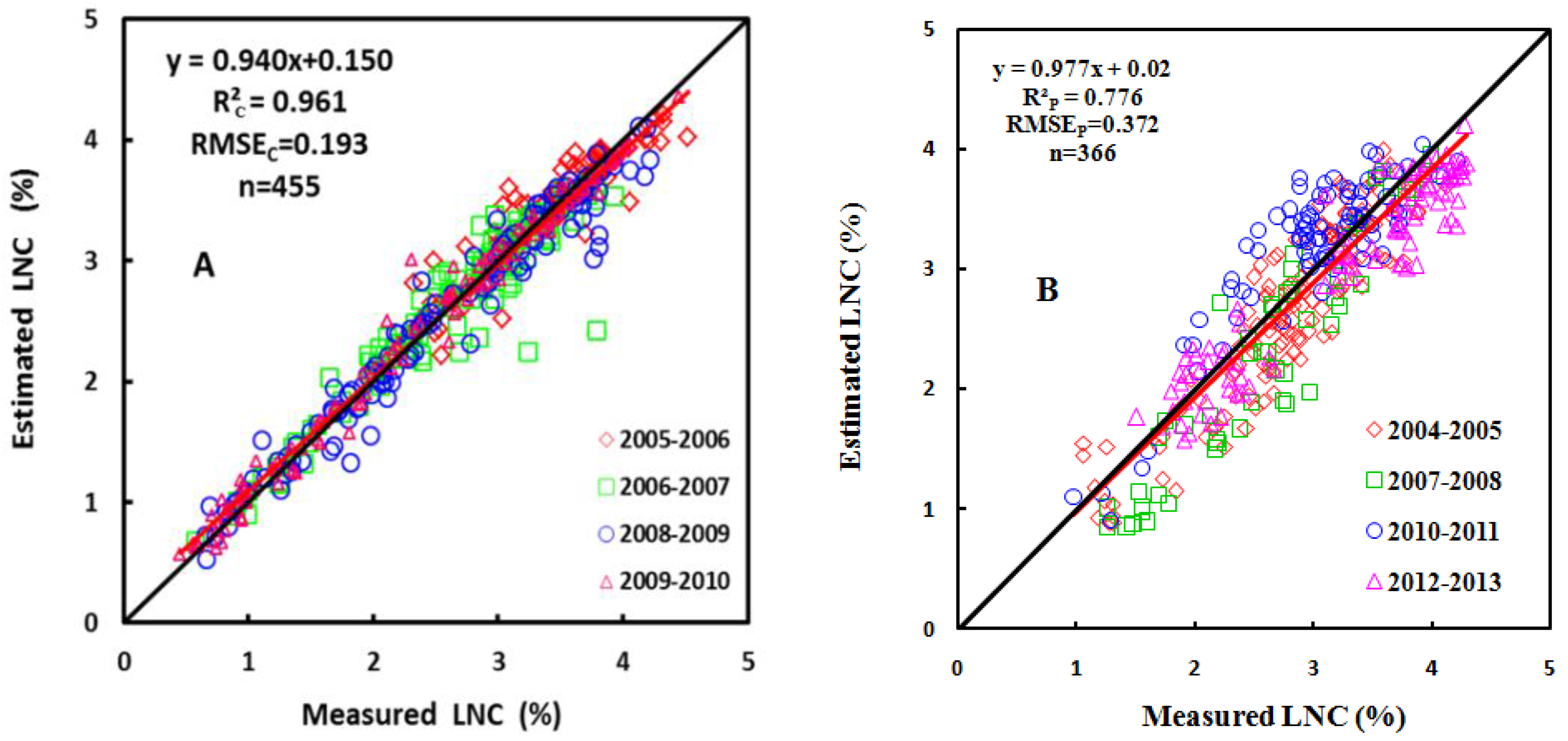
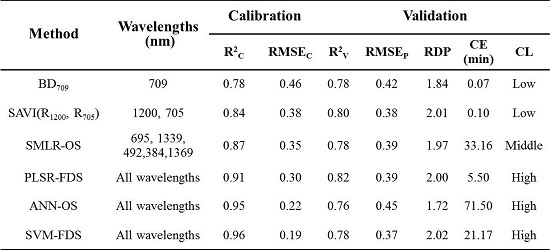
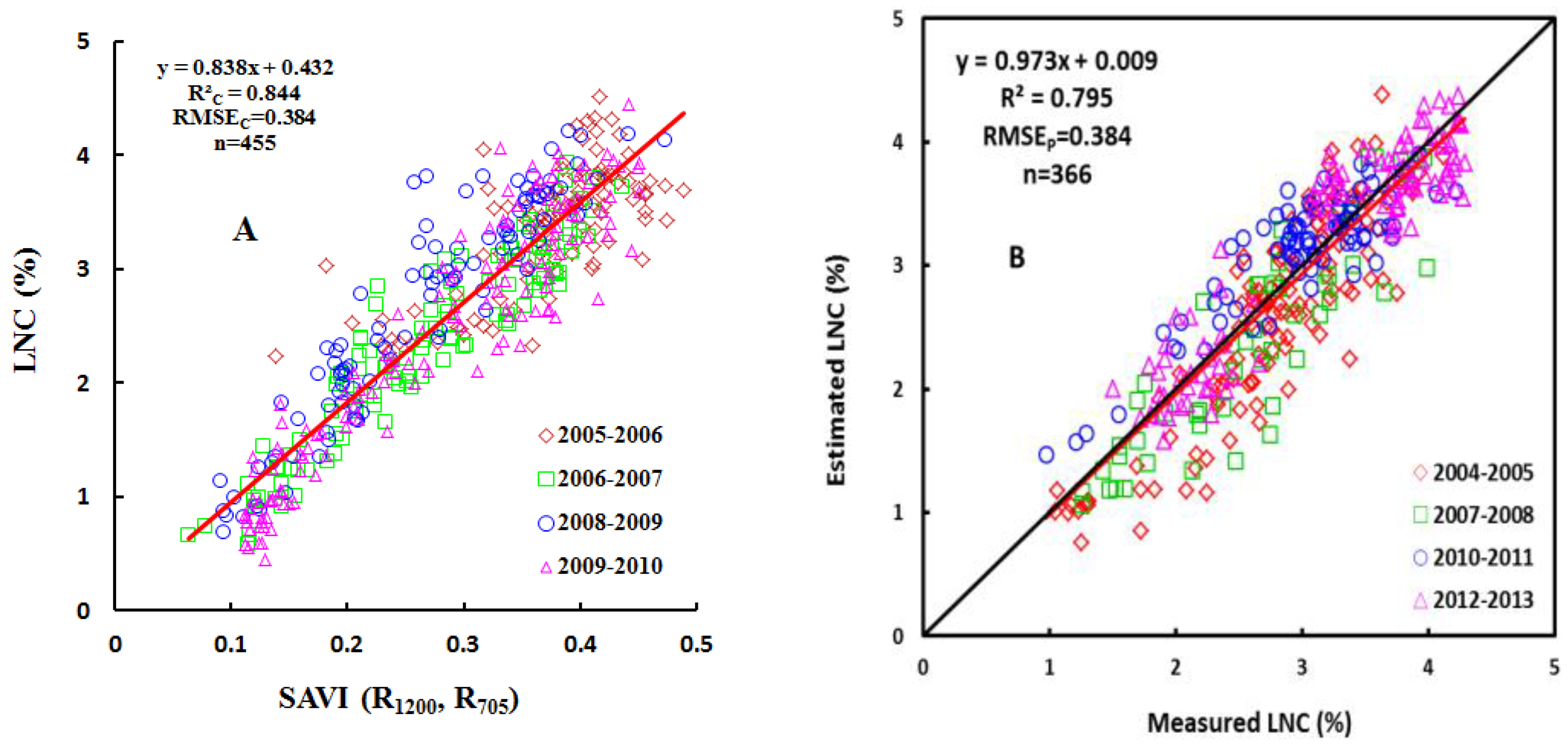
In this study, we demonstrated the performance, advantages, shortcomings, and robustness of six statistical modeling approaches for wheat canopy LNC. The PLSR-FDS, ANN-OS and SVM-FDS methods yield similar accuracies with SVM-FDS as the best if the CE and CL are not considered, however, ANNs and SVMs performed better on calibration set than the validation set which indicate that we should take more caution with the two methods for over-fitting. Except PLS method, the performance for most methods did not enhance when the spectrum were operated by the first derivative. The prediction accuracy was found to be higher when more wavelengths were used, though at the cost of a lower CE. Moreover, the evaluation of the robustness demonstrates that SVMs method may be better suited than the other methods to cope with potential confounding factors for most varieties, ecological site and growth stage. However, when the estimation accuracy, the CE, the number of wavelengths, and the CL of each model are systematically considered for the design of hardware devices, the SAVI(R₁₂₀₀, R₇₀₅) model is found to be the best option for estimating the LNC in wheat. Although it might generally be preferable to make use of the full spectral resolution, our study demonstrated that even with two spectral bands, it is possible to (locally) obtain very good results. Hence, it remains to be proven that the full wavelength spectrum contains substantially more information than do narrow-band vegetation indices.

The current study focused on the six most widely used algorithms for the considered task. The results of this study are of interest to the remote sensing community for the development of improved inversion schemes for hyperspectral applications concerning other types of vegetation using empirical models, such as mapping important vegetation biophysical properties of other crops. The examples provided in this paper may also serve as illustrations of the advantages and disadvantages of empirical models. Although statistical models have been developed and successfully applied across various growth stages, varieties and eco-sites, the use of these methods is not always possible. Those methods in this paper established for vegetation variable retrieval, which are frequently applied in terrestrial bio-physical products, proving a high potential of hyperspectral measurement in the future. Because our study was performed using a specific dataset, our findings necessarily have certain limitations in applicability. In order to develop accurate, robust and fast model with high reliability, practicability and applicability, the next step should be to confirm these findings for a broader range of species and environments. A simulation experiment based on synthetic spectra generated by physically-based radiative transfer model will be conducted. Physical accuracy estimates are mandatory and should be provided using comprehensive validation datasets collected on more various sites and varieties. Except parametric regression and non-parametric regression, the hybrid methods combine generic capability of physically-based methods with flexible and computationally efficient methods should be tested. What is more, the impact of feature selection and randomly generated noise should be considered to study the stability of the developed statistical models to unfavorable measuring conditions with different sites and varieties in the future. Additionally, the theoretical uncertainties of the biophysical parameter products should be analysis in the study. The associated uncertainty estimates also provide information on the success of transporting a locally trained model to other sites and/or observation conditions, which are not intended to replace true accuracy estimates, but instead provide complementary information.

References

1. Clevers, J.G.P.W.; Gitelson, A.A. Remote estimation of crop and grass chlorophyll and nitrogen content using red-edge bands on Sentinel-2 and -3. Int. J. Appl. Earth Obs. Geoinform. 2013, 23, 344–351. [Google Scholar] [CrossRef]
2. Thomas, J.R.; Oerther, G.F. Estimating nitrogen content of sweet pepper leaves by reflectance measurements. Agron. J. 1972, 64, 11–13. [Google Scholar] [CrossRef]
3. Jensen, A.; Lorenzen, B.; Østergaard, H.S.; Hvelplund, E.K. Radiometric estimation of biomass and nitrogen content of barley grown at different nitrogen levels. Int. J. Remote Sens. 1990, 11, 1809–1820. [Google Scholar] [CrossRef]
4. Yoder, B.J.; Pettigrew-Crosby, R.E. Predicting nitrogen and chlorophyll content and concentrations from reflectance spectra (400–2500 nm) at leaf and canopy scales. Remote Sens. Environ. 1995, 53, 199–211. [Google Scholar] [CrossRef]
5. Kokaly, R.; Clark, R.N. Spectroscopic determination of leaf biochemistry using band-depth analysis of absorption features and stepwise multiple linear regression. Remote Sens. Environ. 1999, 67, 267–287. [Google Scholar] [CrossRef]
6. Pinter, P.J.; Hatfield, J.L.; Schepers, J.S.; Barnes, E.M.; Moran, M.S.; Daughtry, C.S.T.; Craig, S.T.; Upchurch, D.R. Remote sensing for crop management. Photogramm. Eng. Remote Sens. 2003, 69, 647–664. [Google Scholar] [CrossRef]
7. Dobermann, A.; Blackmore, S.; Cook, S.E.; Adamchuk, V.I. Precision Farming: Challenges and Future Directions. In Proceedings of the 4th International Crop Science Congress, Brisbane, Australia, 26 September–1 October 2004.
8. Huang, Z.; Turner, B.J.; Dury, S.J.; Wallis, I.R.; Foley, W.J. Estimating foliage nitrogen concentration from HYMAP data using continuum removal analysis. Remote Sens. Environ. 2004, 93, 18–29. [Google Scholar] [CrossRef]
9. Ladha, J.K.; Pathak, H.; Krupnik, T.J.; Six, J.; van Kessel, C. Efficiency of fertilizer nitrogen in cereal production: Retrospects and prospects. Adv. Agron. 2005, 87, 85–156. [Google Scholar]
10. Zhu, Y.; Li, Y.X.; Zhou, D.Q.; Tian, Y.C.; Yao, X.; Cao, W.X. Quantitative relationship between leaf nitrogen concentration and canopy reflectance spectra in rice and wheat. Acta Ecol. Sin. 2006, 26, 3463–3469. [Google Scholar]
11. Haboudane, D.; Tremblay, N.; Miller, J.R.; Vigneault, P. Remote estimation of crop chlorophyll content using spectral indices derived from hyperspectral data. IEEE Trans. Geosci. Remote Sens. 2008, 46, 423–437. [Google Scholar] [CrossRef]
12. Tian, Y.C.; Yao, X.; Yang, J.; Cao, W.X.; Hannaway, D.B.; Zhu, Y. Assessing newly developed and published vegetation indices for estimating rice leaf nitrogen concentration with ground- and space-based hyperspectral reflectance. Field Crops Res. 2011, 120, 299–310. [Google Scholar] [CrossRef]
13. Ecarnot, M.; Compan, F.; Roumet, P. Assessing leaf nitrogen content and leaf mass per unit area of wheat in the field throughout plant cycle with a portable spectrometer. Field Crops Res. 2013, 140, 44–50. [Google Scholar] [CrossRef]
14. Yao, X.; Ren, H.; Cao, Z.; Tian, Y.; Cao, W.; Zhu, Y.; Cheng, T. Detecting leaf nitrogen content in wheat with canopy hyperspectrum under different soil backgrounds. Int. Appl. Earth Obs. Geoinform. 2014, 32, 114–124. [Google Scholar] [CrossRef]
15. Curran, P.J.; Dungan, J.L.; Peterson, D.L. Estimating the foliar biochemical concentration of leaves with reflectance spectrometry. Remote Sens. Environ. 2001, 76, 349–359. [Google Scholar] [CrossRef]
16. Hansen, P.M.; Schjoerring, J.K. Reflectance measurement of canopy biomass and nitrogen status in wheat crops using normalized difference vegetation indices and partial least squares regression. Remote Sens. Environ. 2003, 86, 542–553. [Google Scholar] [CrossRef]
17. Li, Y.X.; Zhu, Y.; Tian, Y.C.; Yao, X.; Qin, X.D.; Cao, W.X. Quantitative relationship between leaf nitrogen concentration and canopy reflectance spectra in wheat. Acta Agron. Sin. 2006, 32, 358–362. [Google Scholar]
18. Darvishzadeh, R.; Skidmore, A.; Atzberger, C. Estimation of vegetation LAI from hyperspectral reflectance data: Effects of soil type and plant architecture. Int. J. Appl. Earth Obs. Geoinform. 2008, 10, 358–373. [Google Scholar] [CrossRef]
19. Darvishzadeh, R.; Skidmore, A.; Schlerf, M.; Atzberger, C.; Corsi, F.; Cho, M. LAI and chlorophyll estimation for a heterogeneous grassland using hyperspectral measurements. ISPRS J. Photogramm. 2008, 63, 409–426. [Google Scholar] [CrossRef]
20. Vigneau, N.; Ecarnot, M.; Rabatel, G.; Roumet, P.; Roumet, P. Potential of field hyperspectral imaging as a non-destructive method to assess leaf nitrogen content in wheat. Field Crops Res. 2011, 122, 25–31. [Google Scholar] [CrossRef]
21. Clark, R.N.; Roush, T.L. Reflectance spectroscopy: Quantitative analysis techniques for remote sensing applications. J. Geophys. Res. 1984, 89, 6329–6340. [Google Scholar] [CrossRef]
22. Kokaly, R.F. Investigating a physical basis for spectroscopic estimates of leaf nitrogen concentration. Remote Sens. Environ. 2001, 75, 153–161. [Google Scholar] [CrossRef]
23. Mutanga, O.; Skidmore, A.K.; Prins, H.H.T. Predicting in situ pasture quality in the Kruger National Park, South Africa, using continuum-removed absorption features. Remote Sens. Environ. 2004, 89, 393–408. [Google Scholar] [CrossRef]
24. Gitelson, A.; Merzlyak, M.N. Spectral reflectance changes associated with autumn senescence of Aesculus hippocastanum L. and Acer platanoides L. leaves. Spectral features and relation to chlorophyll estimation. J. Plant Physiol. 1994, 143, 286–292. [Google Scholar] [CrossRef]
25. Chen, P.F.; Wang, J.S.; Peng, P. Remote detection of wheat grain protein content using nitrogen nutrition index. Soc. Agric. Eng. 2011, 9, 75–80. [Google Scholar]
26. Yao, X.; Zhu, Y.; Tian, Y.C.; Feng, W.; Cao, W.X. Research of optimum hyperspectral vegetation indices on monitoring the nitrogen content in wheat leaves. Sci. Agric. Sin. 2009, 42, 2716–2725. [Google Scholar]
27. Hatchell, D. (ASD) Technical Guide; Analytical Spectral Devices. Inc.: Boulder, CO, USA, 1999. [Google Scholar]
28. Lin, F.F.; Qiu, L.F.; Deng, J.S.; Shi, Y.Y.; Chen, L.S.; Wang, K. Investigation of SPAD meter-based indices for estimating rice nitrogen status. Comput. Electron. Agric. 2010, 71, S60–S65. [Google Scholar] [CrossRef]
29. Cao, Q.; Miao, Y.; Wang, H.; Huang, S.; Cheng, S.; Khosla, R.; Jiang, R. Non-destructive estimation of rice plant nitrogen status with Crop Circle multispectral active canopy sensor. Field Crops Res. 2013, 154, 133–144. [Google Scholar] [CrossRef]
30. Cao, Q.; Miao, Y.; Feng, G.; Gao, X.; Li, F.; Liu, B.; Yue, S.; Cheng, S.; Ustin, S.L.; Khosla, R.; et al. Active canopy sensing of winter wheat nitrogen status: An evaluation of two sensor systems. Comput. Electron. Agric. 2015, 112, 54–67. [Google Scholar] [CrossRef]
31. Savitzky, A.; Golay, M.J.E. Smoothing and differentiation of data by simplified least squares procedures. Anal. Chem. 1964, 36, 1627–1632. [Google Scholar] [CrossRef]
32. Bolster, K.L.; Martin, M.E.; Aber, J.D. Determination of carbon fraction and nitrogen concentration in tree foliage by near infrared reflectances: A comparison of statistical methods. Can. J. For. Res. 1996, 26, 590–600. [Google Scholar] [CrossRef]
33. Grossman, Y.L.; Ustin, S.L.; Jacquemoud, S.; Sanderson, E.W.; Schmuck, G.; Verdebout, J. Critique of stepwise multiple linear regression for the extraction of leaf biochemistry information from leaf reflectance data. Remote Sens. Environ. 1996, 56, 182–193. [Google Scholar] [CrossRef]
34. Yu, K.; Li, F.; Gnyp, M.L.; Miao, Y.; Bareth, G.; Chen, X. Remotely detecting canopy nitrogen concentration and uptake of paddy rice in the Northeast China Plain. ISPRS J. Photogramm. 2013, 78, 102–115. [Google Scholar] [CrossRef]
35. Farifteh, J.; van der Meer, F.; Atzberger, C.; Carranza, E.J.M. Quantitative analysis of salt-affected soil reflectance spectra: A comparison of two adaptive methods (PLSR and ANN). Remote Sens. Environ. 2007, 110, 59–78. [Google Scholar] [CrossRef]
36. Brown, M.P.; Grundy, W.N.; Lin, D.; Cristianini, N.; Sugnet, C.W.; Furey, T.S.; Ares, M.; Haussler, D. Knowledge-based analysis of microarray gene expression data by using support vector machines. Proc. Natl. Acad. Sci. USA 2000, 97, 262–267. [Google Scholar] [CrossRef] [PubMed]
37. Gill, M.K.; Asefa, T.; Kemblowski, M.W.; McKee, M. Soil moisture prediction using support vector machines. J. Am. Water Resour. Assoc. 2006, 42, 1033–1046. [Google Scholar] [CrossRef]
38. Lin, G.; Chen, G.; Wu, M.; Chou, Y. Effective forecasting of hourly typhoon rainfall using support vector machines. Water Resour. Res. 2009, 45, W08440. [Google Scholar] [CrossRef]
39. Kalra, A.; Ahmad, S. Using oceanic-atmospheric oscillations for long lead time streamflow forecasting. Water Resour. Res. 2009, 45, W03413. [Google Scholar] [CrossRef]
40. Yang, X.; Huang, J.; Wu, Y.; Wang, J.; Wang, P.; Wang, X.; Huete, A.R. Estimating biophysical parameters of rice with remote sensing data using support vector machines. Sci. China Life Sci. 2011, 54, 272–281. [Google Scholar] [CrossRef] [PubMed]
41. Wang, Y.; Huang, J.F.; Wang, F.M.; Liu, Z.Y. Predicting nitrogen concentrations from hyperspectral reflectance at leaf and canopy for rape. Guang Pu 2008, 28, 273–277. (In Chinese) [Google Scholar] [PubMed]
42. Filella, I.; Peñuelas, J. The red edge position and shape as indicators of plant chlorophyll content, biomass and hydric status. Int. J. Remote Sens. 1994, 15, 1459–1470. [Google Scholar] [CrossRef]
43. Mauser, W.; Bach, H. Imaging spectroscopy in hydrology and agriculture-determination of model parameters. In Imaging Spectrometry––A Tool for Environmental Observations; Hill, J., Megier, J., Eds.; Kluwer Academic Publishing: Dordrecht, The Netherlands, 1995; pp. 261–283. [Google Scholar]
44. Johnson, L.F.; Billow, C.R. Spectrometry estimation of total nitrogen concentration in Douglas-fir foliage. Int. J. Remote Sens. 1996, 17, 489–500. [Google Scholar] [CrossRef]
45. Mutanga, O.; Skidmore, A.K. Narrow band vegetation indices solve the saturation problem in biomass estimation. Int. J. Remote Sens. 2004, 25, 1–16. [Google Scholar] [CrossRef]
46. Chatterjee, S.; Price, B. Regression Analysis by Example; Wiley: New York, NY, USA, 1977. [Google Scholar]
47. Geladi, P.; Kowalski, B.R. Partial least-squares regression: A tutorial. Anal. Chim. Acta 1986, 185, 1–17. [Google Scholar] [CrossRef]
48. Esbensen, K.H.; Guyot, D.; Westad, F.; Houmøller, L.P. Multivariate Data Analysis—In Practice, 5th ed.; CAMO Software: Oslo, Norway, 2010; pp. 241–293. [Google Scholar]
49. Ehsani, M.R.; Upadhyaya, S.K.; Slaughter, D.; Shafii, S.; Pelletier, M. A NIR technique for rapid determination of soil mineral nitrogen. Precis. Agric. 1999, 1, 219–236. [Google Scholar] [CrossRef]
50. Atkinson, P.M.; Tatnall, A.R.L. Introduction neural networks in remote sensing. Int. J. Remote Sens. 1997, 18, 699–709. [Google Scholar] [CrossRef]
51. Vapnik, V.N. Statistical Learning Theory; John Wiley & Sons Inc.: New York, NY, USA, 1998. [Google Scholar]
52. Cortes, C.; Vapnik, V. Support-vector networks. Mach. Learn. 1995, 20, 273–297. [Google Scholar] [CrossRef]
53. Chang, C.; Laird, D.A.; Mausbach, M.J.; Hurburgh, C.R. Near infrared reflectance spectroscopy: Principal components regression analysis of soil properties. Soil Sci. Soc. Am. J. 2001, 65, 480–490. [Google Scholar] [CrossRef]
54. Rondeaux, G.; Steven, M.; Baret, F. Optimization of soil-adjusted vegetation indices. Remote Sens. Environ. 1996, 55, 95–107. [Google Scholar] [CrossRef]
55. Gitelson, A.A.; Merzlyak, M.N. Quantitative estimation of chlorophyll a using reflectance spectra: Experiments with autumn chestnut and maple leaves. J Photochem Photobiol(B). 1994, 22, 247–252. [Google Scholar] [CrossRef]
56. Wang, W.; Yao, X.; Yao, X.F.; Tian, Y.C.; Liu, X.J.; Ni, J.; Cao, W.X.; Zhu, Y. Estimating leaf nitrogen concentration with three-band vegetation indices in rice and wheat. Field Crops Res. 2012, 129, 90–98. [Google Scholar] [CrossRef]
57. Sims, D.A.; Gamon, J.A. Relationships between leaf pigment content and spectral reflectance across a wide range of species, leaf structures and developmental stages. Remote Sens. Environ. 2002, 81, 331–354. [Google Scholar] [CrossRef]
58. Lamb, D.W.; Steyn-Ross, M.; Schaare, P.; Hanna, M.M.; Silvester, W.; Steyn-Ross, A. Estimating leaf nitrogen concentration in ryegrass (Lolium spp.) pasture using the chlorophyll red-edge: Theoretical modelling and experimental observations. Int. J. Remote Sens. 2002, 23, 3619–3648. [Google Scholar] [CrossRef]
59. Jongschaap, R.E.E.; Booij, R. Spectral measurements at different spatial scales in potato: Relating leaf, plant and canopy nitrogen status. Int. J. Appl. Earth Obs. Geoinform. 2004, 5, 205–218. [Google Scholar] [CrossRef]
60. Atzberger, C.; Guérif, M.; Baret, F.; Werner, W. Comparative analysis of three chemometric techniques for the spectroradiometric assessment of canopy chlorophyll content in winter wheat. Comput. Electron. Agric. 2010, 73, 165–173. [Google Scholar] [CrossRef]
61. Pan, W.C.; Li, S.K.; Wang, K.R.; Xiao, H.; Chen, B.; Wang, F.Y.; Su, Y.; Chen, J.L.; Lai, J.C.; Huang, F.D. Monitoring soil nitrogen and plant nitrogen based on hyperspectral of cotton canopy. Cotton Sci. 2010, 22, 70–76. [Google Scholar]
62. Qi, X.M.; Zhang, L.D.; Du, X.L.; Song, Z.J.; Zhang, Y.; XU, S.Y. Quantitative analysis using NIR by building PLSR-BP model. Spectrosc. Spectr. Anal. 2003, 23, 870–872. [Google Scholar]
63. Vuolo, F.; Neugebauer, N.; Bolognesi, S.; Atzberger, C.; D’Urso, G. Estimation of leaf area index using DEIMOS-1 data: Application and transferability of a semi-empirical relationship between two agricultural areas. Remote Sens. 2013, 5, 1274–1291. [Google Scholar] [CrossRef]
64. Rivera, J.; Verrelst, J.; Delegido, J.; Veroustraete, F.; Moreno, J. On the semi-automatic retrieval of biophysical parameters based on spectral index optimization. Remote Sens. 2014, 6, 4927–4951. [Google Scholar] [CrossRef]
65. Tian, Y.; Gu, K.; Chu, X.; Yao, X.; Cao, W.; Zhu, Y. Comparison of different hyperspectral vegetation indices for canopy leaf nitrogen concentration estimation in rice. Plant Soil 2014, 376, 193–209. [Google Scholar] [CrossRef]