Article

Impact of Land Cover Change Induced by a Fire Event on the Surface Energy Fluxes Derived from Remote Sensing

1
Applied Physics Department, University of Castilla-La Mancha, Campus University,16071 Cuenca, Spain
2
Applied Physics Department, University of Castilla-La Mancha, Avda. España s/n, 2071 Albacete, Spain
3
Earth Physics and Thermodynamics Department, University of Valencia, C/Dr. Moliner 50, 46100 Burjassot, Spain
*
Author to whom correspondence should be addressed.
These authors contributed equally to this work.
Remote Sens. 2015, 7(11), 14899-14915; https://doi.org/10.3390/rs71114899
Submission received: 10 August 2015 / Revised: 11 October 2015 / Accepted: 29 October 2015 / Published: 6 November 2015

Abstract

:
Forest fires affect the natural cycle of the vegetation, and the structure and functioning of ecosystems. As a consequence of defoliation and vegetation mortality, surface energy flux patterns can suffer variations. Remote sensing techniques together with surface energy balance modeling offer the opportunity to explore these changes. In this paper we focus on a Mediterranean forest ecosystem. A fire event occurred in 2001 in Almodóvar del Pinar (Spain) affecting a pine and shrub area. A two-source energy balance approach was applied to a set of Landsat 5-TM and Landsat 7-EMT+ images to estimate the surface fluxes in the area. Three post-fire periods were analyzed, six, seven, nine, and 11 years after the fire event. Results showed the regeneration of the shrub area in 6–7 years, in contrast to the pine area, where an important decrease in evapotranspiration, around 1 mm·day−1, remained. Differences in evapotranspiration were mitigated nine and 11 years after the fire in the pine area, whereas significant deviations in the rest of the terms of the energy balance equation were still observed. The combined effect of changes in the vegetation structure and surface variables, such as land surface temperature, albedo, or vegetation coverage, is responsible for these variations in the surface energy flux patterns.

Graphical Abstract

1. Introduction

The management of the water resources benefits from a good characterization of the hydrological processes. Particularly, the soil-vegetation-atmosphere energy exchanges are the basis of an accurate hydrological balance. Energy balance and evapotranspiration are altered by land cover changes that significantly affect canopy structure and leaf area index [1].
Forest fires affect the landscape, the natural cycle of the vegetation, and the structure and functioning of ecosystems. Fires also modify the surface energy flux patterns and provoke changes in the local and regional meteorology as a consequence. Changes in the ecosystem structure and species composition modify the latent heat flux (LE), directly related to the actual evapotranspiration, and the rest of the terms involved in the energy balance equation. These changes in the local energy balance may persist for decades [2] with an impact depending also on the vegetation regenerating the burnt area.
Several works have summarized the effects of fire events on the energy exchange over different surfaces. For example, Amiro et al. [3] observed a decrease in LE several years following a disturbance in a boreal forest. However, not all works observe a significant decrease in LE, depending on fire intensity, succession rate, and vegetation type. Dore et al. [4] analyzed a burnt pine forest area revegetated by grassland. A slight decrease in LE was observed by these authors in the burnt area. Montes-Helu et al. [5] analyzed the effect of a fire event on the surface energy fluxes in a pine forest in Northern Arizona. Eddy-covariance measurements were used by these authors. Results showed important changes on the energy and water balance 10 years after burning [5]. Rocha et al. [6] analyzed the change on surface energy exchange and temperature in a burnt arctic tundra area using eddy covariance data. The analysis in [6] was operated along the three years following the fire event and at different burn severity gradients (severe and moderate). These authors observed higher latent heat fluxes in the burnt area, and no change in sensible heat flux during the first two years followed by lower values in the burnt area after the third year. In [1] Clark et al. analyzed the impact of land cover change on energy exchange and evapotranspiration from eddy covariance measurements. They analyzed a burnt area and also an area that had been defoliated by insects. Both effects reduce leaf area and evapotranspiration [1].
As shown above, the majority of the literature discussing the effects of fires on surface fluxes is based on ground measurements. While there are numerous techniques, such as eddy-covariance, for collecting in situ measurements of the surface energy fluxes, the measurements are highly localized. Thus, capturing the spatial variability of the surface fluxes would require a high-density network of sensor systems, an approach that is impractical. Multi-temporal remote sensing techniques have been effectively employed to quantify patterns of variation in space and time, and then assess and monitor landscape changes in a rapid and cost-effective manner [7,8,9,10]. Different surface variables and parameters can be extracted from the combination of the multi-spectral information contained in a satellite image, with a detail level dependent on the spatial resolution of the sensor used. Lentile et al. [7] includes a comprehensive bibliographic revision of works using remote sensing techniques to analyze post-fire effects on surface temperature, surface reflectance, vegetation consumption, vegetation mortality, etc. Since the 1980s, different techniques have been developed for data acquired from AVHRR, MODIS, SPOT, Landsat, or ASTER. Most of these works are based on the use of information on spectral changes due to burning. López and Caselles [8] demonstrated the usefulness of using a reference area, and studied the effect of fires on surface temperature and reflectivity values from Landsat TM images. Díaz-Delgado [9] analyzed the interactions between fire severity and plant regeneration after fire by means of NDVI measurements from Landsat TM and MSS images. Satellite remote sensing also allows the estimation of surface energy fluxes at regional scale. Sensors providing the high spatial resolution required to distinguish different fields or land uses within a scene have a poor revisit frequency. Furthermore, note that satellite remote sensing provides instantaneous information of the surface energy balance at the specific time of the sensor overpass. Daily estimates of the surface energy fluxes from these instantaneous data require further assumptions. Nevertheless, remote sensing techniques are convenient to carry out long-term studies covering large areas.
Very few works in the literature introduce the use of remote sensing techniques to study the effect of fires on the surface energy balance. Ha et al. [10] used the MODIS evapotranspiration (ET) product to monitor a burnt forest area over four years, and compared results with eddy covariance measurements. These authors concluded that MODIS ET estimates need to be improved through use of higher resolution products. Wang et al. [11] used a modified version of the Surface Energy Balance Algorithm for Land (SEBAL) to monitor vegetation ET changes between burnt and unburnt areas from two ASTER images. In this paper we move forward and show the potential of the combination between surface energy balance and medium-resolution remote sensing techniques to analyze the effects of land cover changes on the surface energy flux patterns.
Land surface temperature estimated from satellite images is a key input in the estimation of energy fluxes. Monteith [12] proposed a single source model to obtain the evapotranspiration, but the application of this model to partial canopy cover conditions has important limitations [13]. As an alternative, two-source (soil + vegetation) models have been developed to accommodate partial canopy cover conditions considering energy exchange between soil and canopy components [14,15,16,17]. In this work we use the Simplified Two-Source Energy Balance (STSEB) model proposed by Sánchez et al. [17,18]. The STSEB approach has been tested under different surface conditions. Sánchez et al. [19] showed its applicability at a regional scale using remote sensing and local meteorological data.
The aim of this paper is to study the evolution in the patterns of the principal terms of the surface energy balance after a fire event in a Mediterranean forest ecosystem, using remote sensing techniques. This is newness beyond the recurrent analysis of post-fire effects from satellite data focused on surface reflectivity and temperature values. A site located in Almodóvar del Pinar, Cuenca (Spain), was selected. This area was affected by a forest fire in the summer of 2001. This fire destroyed 172 ha of Maritime pine-holm oak mixed forest and shrubland. This area became an intensive study site after the fire. Satellite image information was used as inputs into a surface energy balance model to quantify the effect of this forest fire in terms of net radiation, soil and sensible heat fluxes, and latent heat flux in the two land cover classes dominant in the area, mature forest, and shrubland. With this aim, the STSEB model [17] was first applied to a set of Landsat 5-TM images corresponding to the period July 2007–July 2008 (6–7 years after the fire). A second set of Landsat 5-TM and 7-ETM+ images was analyzed for the summer of 2010 (nine years after the fire). The study was completed with a third set of Landsat 7-ETM+ images for the summer of 2012 (11 years after the fire).

2. Materials and Methods

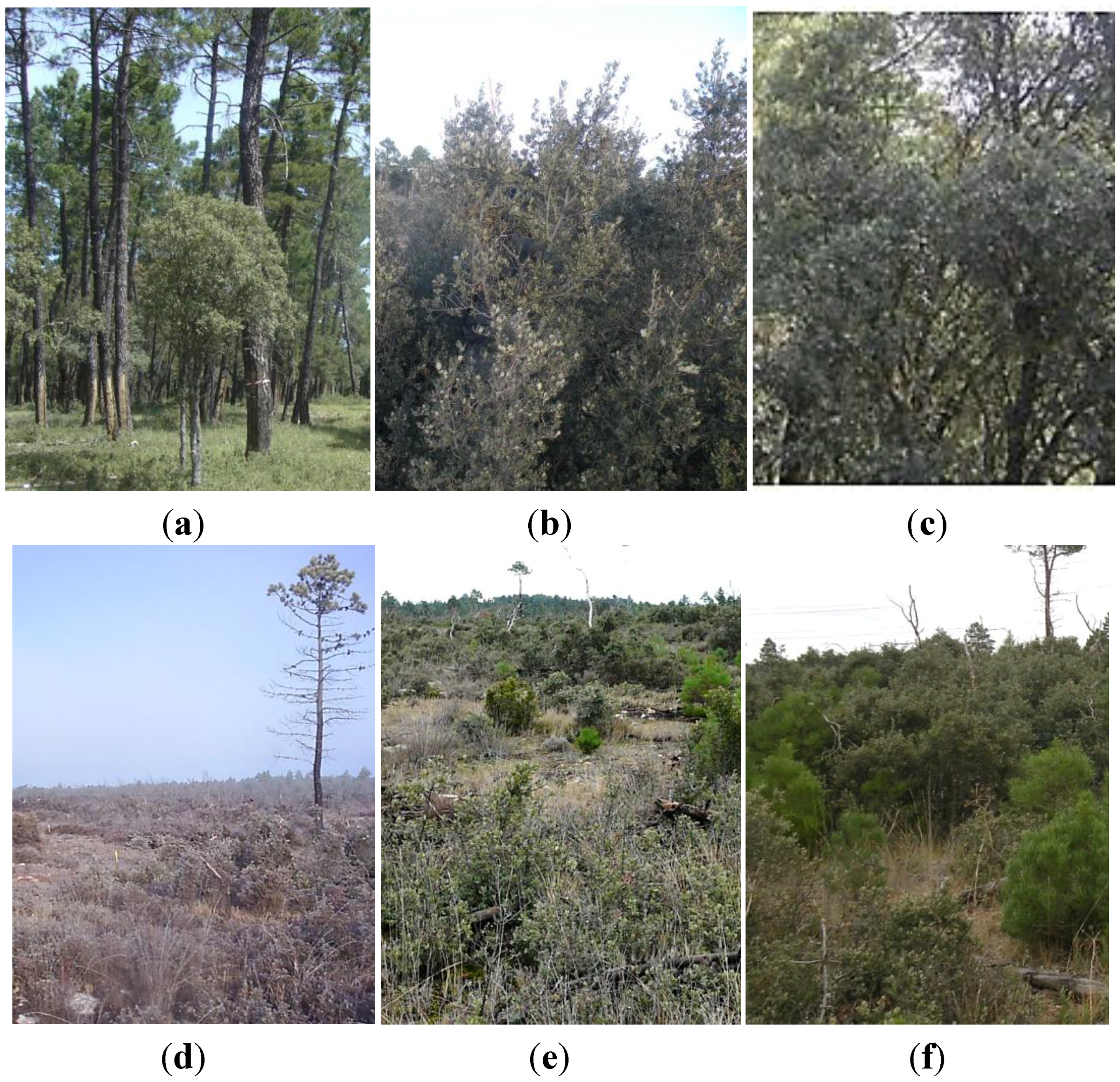
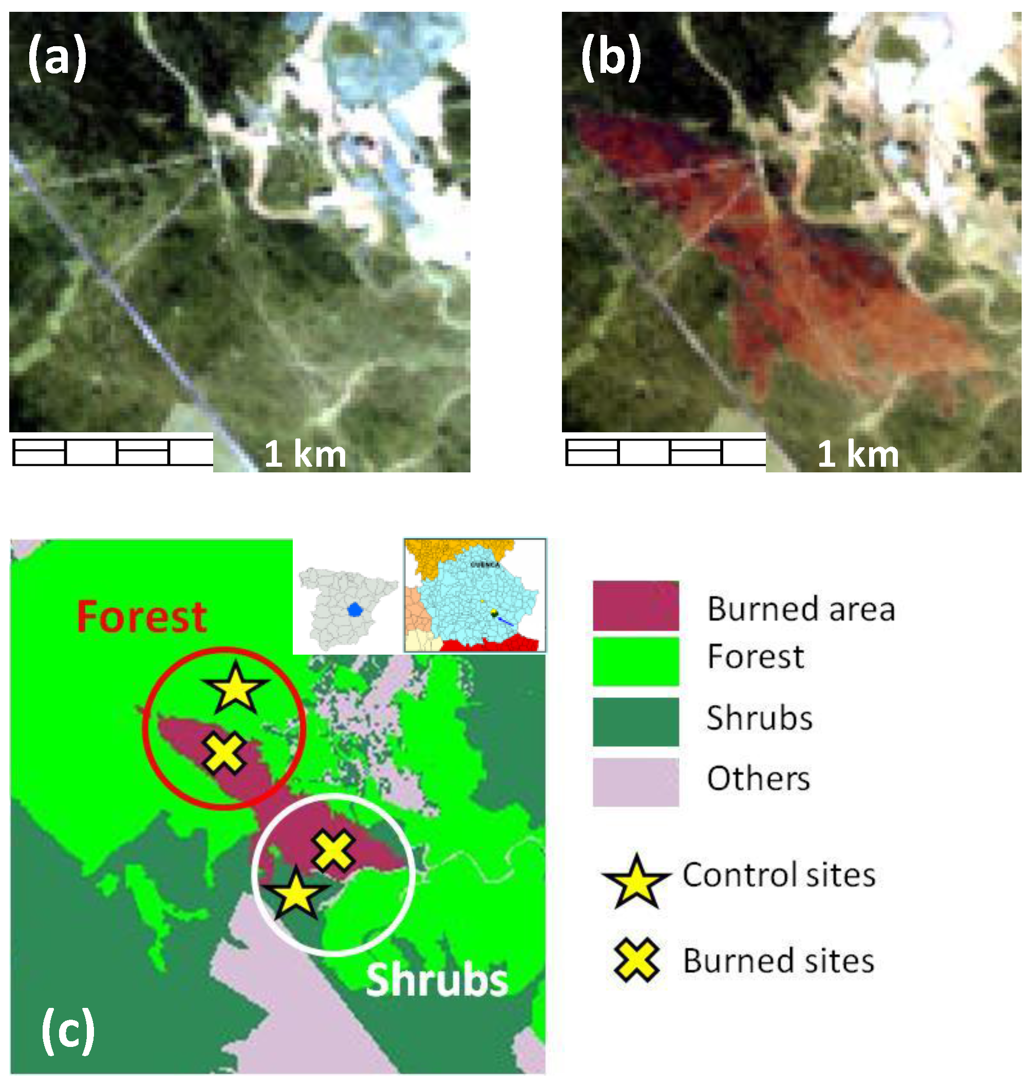
2.1. Study Site and Data

The two study sites, forest and shrub areas, were situated in the adjacent locations of Almodóvar del Pinar and Campillo de Altobuey, respectively (Cuenca province, 1°51′W, 39°40′S, 1020 m amsl), in Southeastern Spain. This region has a Mediterranean climate, with warm dry summers, and cool winters.
The unburnt shrub area consists of an uneven aged coppice holm oak forest (Figure 1b), naturally regenerated after being affected by a wildfire in August, 1993. The natural vegetation consists of evergreen oak resprouts and other shrubs, such as Juniperus comunis, Sidertis incana, Thymus vulgaris, Helianthemum cinereum, H. hirtum, Santolina chamacyparissus, and Bupleurum fruticescens, and herbaceous plants, such as Linaria glauca, Bombycilaena erecta, Wangenheima lima, Euphorbia exigua, Erophila berna, and Petrorhagia nanteuilii [20].
Figure 1. Overviews of: (a) pine forest control site (Forest_c); (b) shrub control site (shrub_c); (c) mature holm oak site; burnt pine forest area six years (d), nine years (e), and 12 years (f) after the fire.
Remotesensing 07 14899 g001
In the summer of 2001, a wildfire affected a total of 172 ha of which 113 ha corresponded to the forest pines and 59 ha to the coppice holm oak forest (Figure 2). The main tree species in the post-fire community consisted of a very high density of sprouted Holmholm oak (>9000 standards·ha−1). This is a typical succession pattern of the Mediterranean region when the holm oak is present. Holm oak is a mature successional hardwood species that have adapted traits to fire-prone habitats. Therefore, post-fire communities usually show a high tree density which negatively influences the growth and increases the fire risk. Six years after the fire, the burnt stand was composed mainly by adult holm oak stools with a variable number of stems, with a maximum height of 2 m, which were grouped in big coppiced shrubs. In addition to shrubs, such as Sideritis incana L., Thymus vulgaris L., Santolina chamaecyparissus L. and Bupleurum fruticescens L. were also present (Figure 1d). The burnt forest area also included scattered pine saplings (max. 1 m of height). Nine years after the fire the density of pines at the burnt and unburnt forest areas were not significantly different (Table 1). As it occurs with holm oak, maritime pine has also adapted to fire-prone regions and has traits related to plant persistence under recurrent fires. In particular, this species has serotinous cones that release seeds after the fire [21].
Figure 2. L7-ETM+ false color compositions (7,5,3) of the study site before (a) and after the fire (b) for 8 June and 26 July 2001, respectively. Land use map after the fire (c) with indication of the test sites [22].
Remotesensing 07 14899 g002
Table 1. Forest stands variables (mean and standard error) for both the Mediterranean maritime pine (PPr) and the holm oak (Qi), in 2010, for the unburnt site (Forest_c area) and for the burnt site. Data of tree density (trees·ha−1), basal area (m2·ha−1) and crown coverage (%).
Forest_c AreaBurnt Area
QiPPrQiPPr
Tree density (tree·ha−1)260 (40)440 (30)9160 (70)450 (4)
Basal Area (m2·ha−1)2.7 (0.4)22.2 (1.5)2.276 (0.024)0.433 (0.004)
Crown coverage (%)19 (4)58 (7)41 (8)0.4 (0.1)
Six 120 × 120 m2 test sites, three inside and three outside the burnt area perimeter, were selected for this study, as samples of both pine and shrub areas. The CORINE land use classification map [22] was used as a basis for this selection. Test sites outside the fire perimeter were called control sites (_c). Environmental conditions in these control sites mimic those in the test sites inside the burnt perimeter if the fire had not happened. Moreover, we selected a nearby area representative of a mature holm oak forest to analyze the effect of the fire on a future scenario in which pines are replaced by holm oaks as the dominant species (Figure 1f).
A meteorological tower was placed in the Forest_c area. Ambient air temperature and relative humidity were measured at 2 and 20 m height from HMP45C sensors (Vaisala, Helsinki, Finland). Wind speed was recorded at 2 and 20 m height using a 05103 Wind Monitor. Solar radiation was measured at 20 m high with a LI-200SZ pyranometer (LI-COR Inc., Lincoln, Nebraska, USA). At soil level temperature (STS-5031, Geonica S.A., Madrid, Spain) and volumetric soil moisture (ECH2O-20 Decagon Devices Inc., Pullman, Washington, USA) probes were buried at a specific depth under two different land covers. Additionally, a rain gauge (R.M. YOUNG Company, Traverse city, Michigan, USA) was used to monitor rainfall. All data were sampled at 2 s intervals and then averaged and stored every 10 minutes. Data records started in summer 2007 and lasted to early 2013 when, unfortunately, the station had to be dismounted. An eddy-covariance system (Fluxnet ID: ES-AP2) was mounted in this tower to measure the turbulent fluxes at the Forest_c area from 2011 to early 2013. A Bowen station was set up in the forest (burnt) site in September 2007 (Figure 1b) and dismounted in October 2009. A set of soil heat flow transducers (HFP01, Hukseflux, Delft, The Netherlands) were buried at 8 cm depth to measure the soil heat flux.
A set of five Landsat 5-TM scenes was selected for the analysis 6–7 years after the fire event (19 July 2007, 4 August 2007, 28 September 2007, 2 May 2008, 21 July 2008). A second set of mixed Landsat 5-TM and 7-ETM+ images was selected for 2010 (16 May, 1 June, 11, 18, and 27 July). Since Landsat 5 images were no longer available after 2011, 5 Landsat 7-ETM+ were selected for 2012 (29 May, 9 July, 1 August, 10 August, 29 October). The spatial resolution for the visible and near infrared bands (VNIR) is 30 m in both sensors, while it differs for the thermal band (TIR), 120 m and 60 m for TM and ETM+, respectively. Due to the failure of the Scan Line Corrector (SLC) for Landsat 7-ETM+ in 2003, there are some gaps in the images. For this reason the selection of the dates in 2010 and 2012 was limited not only by the cloud coverage but also by the presence of gaps in the different study stands (forest, shrub and mature holm oak). Corrected surface reflectivity values (CDR archive) derived from USGS [23] were used. Brightness temperatures were corrected from atmospheric and emissivity effects according to the methodology described in [19]. The atmospheric profiles required were obtained from the Atmospheric Correction Tool by Barsi et al. [24,25].

2.2. Methodology

The STSEB model is based on the Energy Balance Equation (EBE) of the land surface, which described a system formed by vegetation, soil beneath, and atmosphere:
R n = G + H + L E
where Rn is the net radiation flux (W·m−2), G is the soil heat flux (W·m−2), H is the sensible heat flux (W·m−2), and LE is the latent heat flux (W·m−2) in the atmospheric boundary layer. In the approaches based on the EBE, LE is estimated as a residual from Equation (1).
The instantaneous net radiation can be calculated by establishing a balance between the long-wave and the short-wave radiation:
R n = ( 1 α ) S + ε L s k y ε σ T R 4
where S and Lsky are the solar global radiation (W·m−2) and the incident long-wave radiation (W·m−2), respectively. TR is the radiometric land surface temperature, α is the surface albedo, ε is the surface effective emissivity, and σ is the Stefan-Boltzmann constant. In this paper, α was integrated using the equation [26]:
α = 0.221 ρ 1 + 0.162 ρ 2 + 0.102 ρ 3 + 0.354 ρ 4 + 0.059 ρ 5 + 0.0195 ρ 7
where ρi is the corrected reflectivity for the i band of TM or ETM+.
A simple and operational equation proposed by Valor and Caselles [27] was used to estimate the surface emissivity from the knowledge of the fractional vegetation cover, Pv, and the emissivities of the soil and canopy components, εs and εc, respectively:
ε = ε c P v + ε s ( 1 P v ) ( 1 1.74 P v ) + 1.7372 P v ( 1 P v )
Fractional vegetation cover was obtained though the methodology proposed by Valor and Caselles [28], using the NDVI calculated from the reflectivity values in the red and near-infrared Landsat spectral bands.
The radiative transfer equation was used to calculate TR from the radiance, L, registered by the thermal band (10.4–12.5 µm) of TM and ETM+:
L = [ εB ( T R ) + ( 1 ε ) L ] τ + L
where B(TR) is Planck’s function for temperature TR, and L, L, and τ are the hemispheric downwelling sky radiance, the upwelling sky radiance, and the atmospheric transmisivity, respectively.
The sensible heat flux in the STSEB is separated in two components: soil (Hs) and canopy (Hc), which are weighted by Pv:
H = P v H c + ( 1 P v ) H s
where Hs and Hc are expressed as:
H c = ρ C p T c T a r a h
H s = ρ C p T s T a r a a + r a s
where ρCp is the volumetric heat capacity of air (J·K−1·m−3), Ta is the air temperature at a reference height (K), Tc and Ts are the canopy and soil radiometric temperatures, respectively, rah is the aerodynamic resistance to heat transfer between the canopy and the reference height (m·s−1), raa is the aerodynamic resistance to heat transfer between the point z0+d (z0: roughness length, d: displacement height) and the reference height (m·s−1), ras is the aerodynamic resistance to heat flow in the boundary layer immediately above the soil surface (m·s−1). Canopy height (h) was assigned nominal values, based on ground inspection, using the CORINE land use classification [22] as a basis. Further details about the expressions to estimate the aerodynamic resistances can be seen in [17]
Finally, the instantaneous soil heat flux can be obtained as a fraction of the net radiation [15]:
G = C G ( 1 P v ) R n
Recommended values for CG typically range from 0.15 to 0.40 in the literature [15,29,30] depending on the soil type and moisture, principally. In this work we used a mean value of CG = 0.275 .
The estimation of the diurnal fluxes is based on the relationship between diurnal and instantaneous H and Rn [31]:
H d R n d = H i R n i
where the subscripts i and d refer to instantaneous and daily fluxes, respectively. On a diurnal timescale, G can constitute an important contribution to the EBE [15,21]. However, at a daily scale G can be neglected in Equation (1) [31,32,33], and LE can be obtained from Equations (1) and (9) as:
L E d = R n d R n i ( R n i H i )
Using Equation (10), LEd can be obtained from the instantaneous values of Rn and H at a particular time of day, and the relative net radiation contribution at that time when global radiative exchange is integrated, Rnd/Rni.

3. Results and Discussion

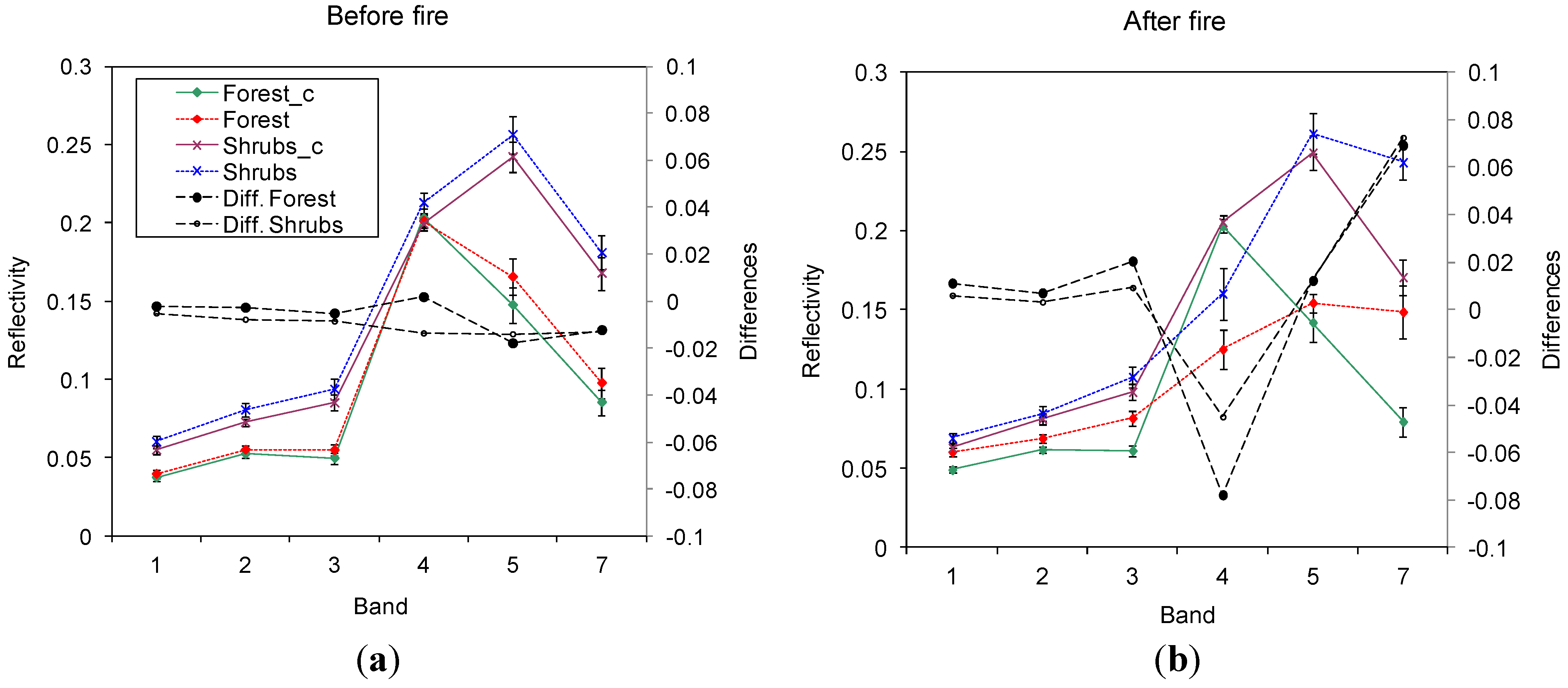
3.1. Assessment of the Control Areas

A comparison between control and fire-affected sites was conducted in order to assess the validity of these control spots as representative of the pre-fire conditions in the burnt sites. Spectral signatures and surface temperature from both sites were compared just before and after the fire on dates 8 June 2001 and 26 July 2001, respectively. Surface reflectivity values, from the six VNIR spectral bands in ETM+, were used for testing. Figure 3a, shows the spectral response of both sites prior the fire. Differences between control and fire affected areas are negligible. On the contrary, important differences are observed post-fire (Figure 3b), with an increase in reflectivity for band seven (SWIR), and a decrease in band four (NIR), consequences of the vegetation disappearance. In terms of land surface temperature, differences before the fire between control and fire-affected sites were 1.3 ± 0.8 °C and −1.1 ± 1.1 °C for the forest and shrub sites, respectively. After the fire, these differences increased up to 12.8 ± 1.7 °C and 7.5 ± 1.3 °C for the forest and shrub sites, respectively.
Figure 3. Average reflectivity values, and their corresponding error bars, for each one of the selected areas (colored lines), and differences between fire-affected sites and their corresponding control areas (black lines): (a) before the fire, and (b) after the fire. Spectral ranges for the different bands: (1) 0.45–0.52 µm, (2) 0.52–0.60 µm, (3) 0.63–0.69 µm, (4) 0.76–0.9 µm, (5) 1.55–1.75 µm, (7) 2.08–2.35 µm.
Remotesensing 07 14899 g003

3.2. Comparison with Observed Fluxes

Figure 4 shows, as an example, maps generated from the 1 August 2012 image. Seven of the scenes available for the present study were concurrent with ground flux measurements. Results for these dates were compared with values registered in the Bowen and eddy-covariance stations located in the forest and forest_c sites, respectively (Table 2). Average values of modeled fluxes were calculated in a 5 × 5 pixel window centered in the location of the ground stations. Relative errors of 4% (22 W·m−2), 40% (30 W·m−2), 14% (60 W·m−2), and 40% (60 W·m−2) are obtained for Rn, G, H, and LE, respectively, at an instantaneous scale. In general, these errors decrease at a daily scale showing average values of 3% (5 W·m−2), 18% (23 W·m−2), and 30% (14 W·m−2, ~0.5 mm·day−1) for Rn, H, and LE, respectively. These results are in agreement to previous assessments of the STSEB model under a variety of land uses and environmental conditions [17,18,19].
Sánchez et al. [17,18] conducted a detailed sensitivity analysis of the resultant fluxes to typical uncertainties in the STSEB inputs. These authors showed that meteorological variables are the main error source. Ta shows the greatest impact on H, with sensitivity values around 20%–30%. Net radiation is mainly affected by S and Lsky, showing sensitivity values of 10%–15%. As a result, uncertainties in LE outputs range 15%–30%. According to the methodology described above, horizontal homogeneity in the meteorological parameters is assumed for burnt and unburnt sites. As a consequence, model errors obtained in this local assessment (Table 2) produced by uncertainties in the meteorological variables tend to be minimized after computing burnt-unburnt differences.
Figure 4. Maps of instantaneous values of (a) Pv, (b) TR (°C), (c) Rn (W·m−2), (d) G (W·m−2), (e) H (W·m−2), and (f) LE (W·m−2), obtained from the L7-TM image corresponding to the date 1 August 2012. In this figure the SLC gaps have been filled, only for display purposes using the ENVI v4.7 Landsat Gapfill tool with the “single file gap triangulation” method selected.
Remotesensing 07 14899 g004
Table 2. Quantitative analysis of the comparison between modeled (Mod.) and observed (Obs.) values of the different surface energy fluxes at the forest and forest_c sites, for years 2007 and 2008 (three dates) and 2012 (four dates), respectively.
Rni (W·m−2)Gi (W·m−2)Hi (W·m−2)LEi (W·m−2)Rnd (W·m−2)Hd (W·m−2)LEd (W·m−2)
ObsModObsModObsModObsModObsModObs.Mod.Obs.Mod.
28 September 200749054012098310360648212013092872843
2 May 2008630640130130390320110200190190120937096
21 June 20086506301001104303701301502002001201208079
28 May 201269067096664505001501102102001101505351
8 July 20126506504682500550100212102101701804332
31 July 201263063029725004501301001801801501304052
9 August 201259058022813304001601001501501301003247
Mean62062080904204201201101801801301205060
Bias1.4−46−120.1−58
RMSE2230606052314
RMSE* (%)440144031830
*: Relative error of the differences, in percentage, calculated as the ration between RMSE (W·m−2) and mean obs. (W·m−2).

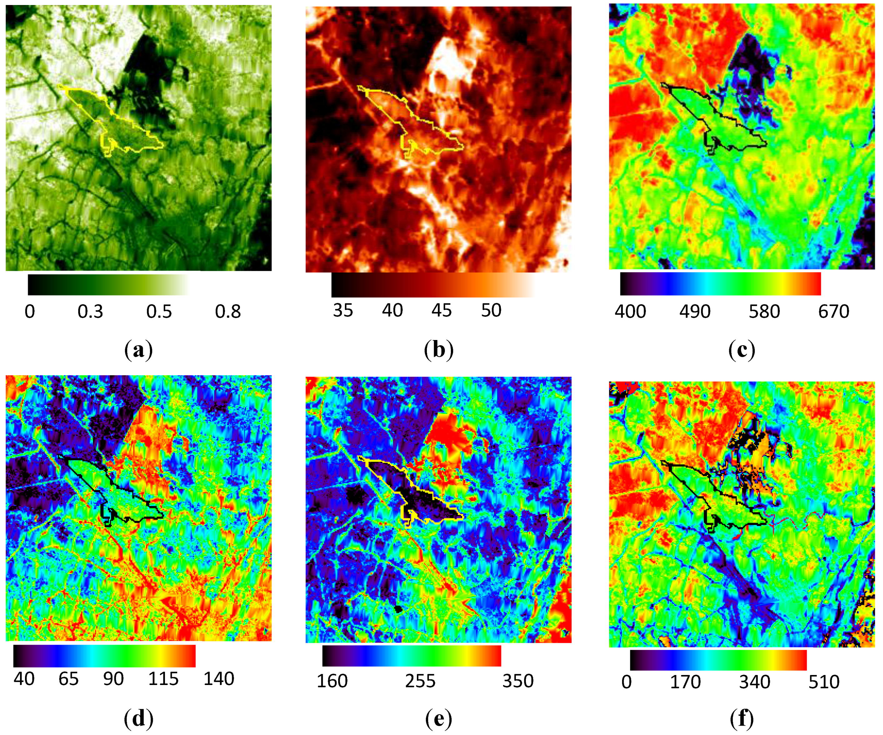
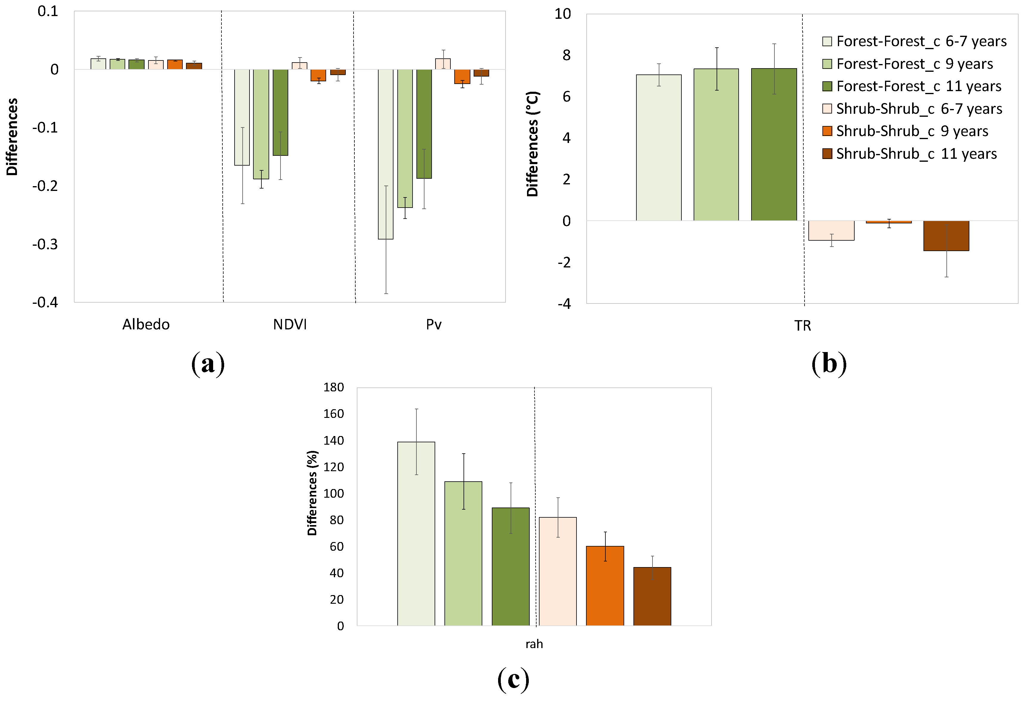
3.3. Analysis of the Fire Effect

3.3.1. Effects on Surface Parameters

Average values of the fluxes and principal inputs in the model were obtained for each one of the test sites and dates, 6–7, 9, and 11 years after the fire (Table 3).
Table 3. Comparison of the results for control and burnt sites and both, forest and shrub areas, for years 2007, 2008, 2010, and 2012. Listed values correspond to the average of the results obtained for the five dates considered in each period.
Postfire YearsSiteAlbedoNDVIPvTR (°C)rah
(s·m−1)
Rni GiHiLEiRndHdLEd
(W·m−2)
6–7Forest_c0.110.470.6028.1136807220040020061140
Forest0.130.300.3134.43162012036015018011078
Shrubs_c0.120.310.3233.0176401103202101909396
Shrubs0.140.320.3432.43163011035018019010086
9Forest_c0.110.570.6235.3207507632035020091110
Forest0.120.400.4142.44168011022035019061130
Shrubs_c0.110.430.4440.92670011028031019079110
Shrubs0.130.410.4240.94169011022036019060130
11Forest_c0.110.550.6030.7135907042011016012043
Forest0.120.390.4036.925540903301201509254
Shrubs_c0.120.390.4036.818550914006715011037
Shrubs0.130.390.3935.525550923301301509255
Figure 5. Average values of the differences between burnt and unburnt (control_c) areas in terms of the main surface parameters: (a) albedo, NDVI, Pv, (b) TR, and (c) rah, for all study sites and dates. Error bars represent the standard deviations of the averages.
Remotesensing 07 14899 g005
Figure 5 shows the average values for albedo, NDVI, Pv, TR, and rah. Based on the differences plotted in this figure, six years after the fire the shrubland almost recovers to its prior fire stage, in terms of most of the surface parameters. On the contrary, important differences in NDVI and Pv persist even 11 years after the fire in the forest area. A similar effect can be observed in terms of surface temperature (Figure 5b). In the forest site TR values are, on average, 7 °C higher in the burnt area, whereas in the shrubs site, this difference is minimum ( ~1°C). Note this effect in surface temperature remains after 11 years. The change in the surface vegetation structure was parameterized through the aerodynamic resistance rah plotted in Figure 5c. To account for the large variability of this parameter as a function of the wind speed, differences are shown in percentage relative to the absolute values obtained for each control site. Average increments of about 140% and 80% are observed in rah values of forest and shrubs areas, respectively, 6–7 years after the fire. These values reduce along the years, still reaching about 80% and 40% for forest and shrubs areas, respectively, after 12 years.

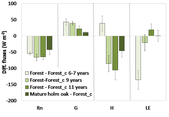
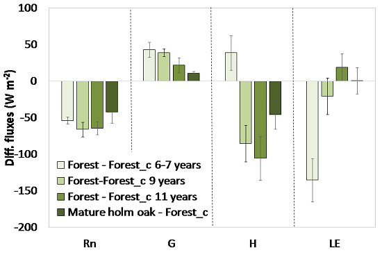
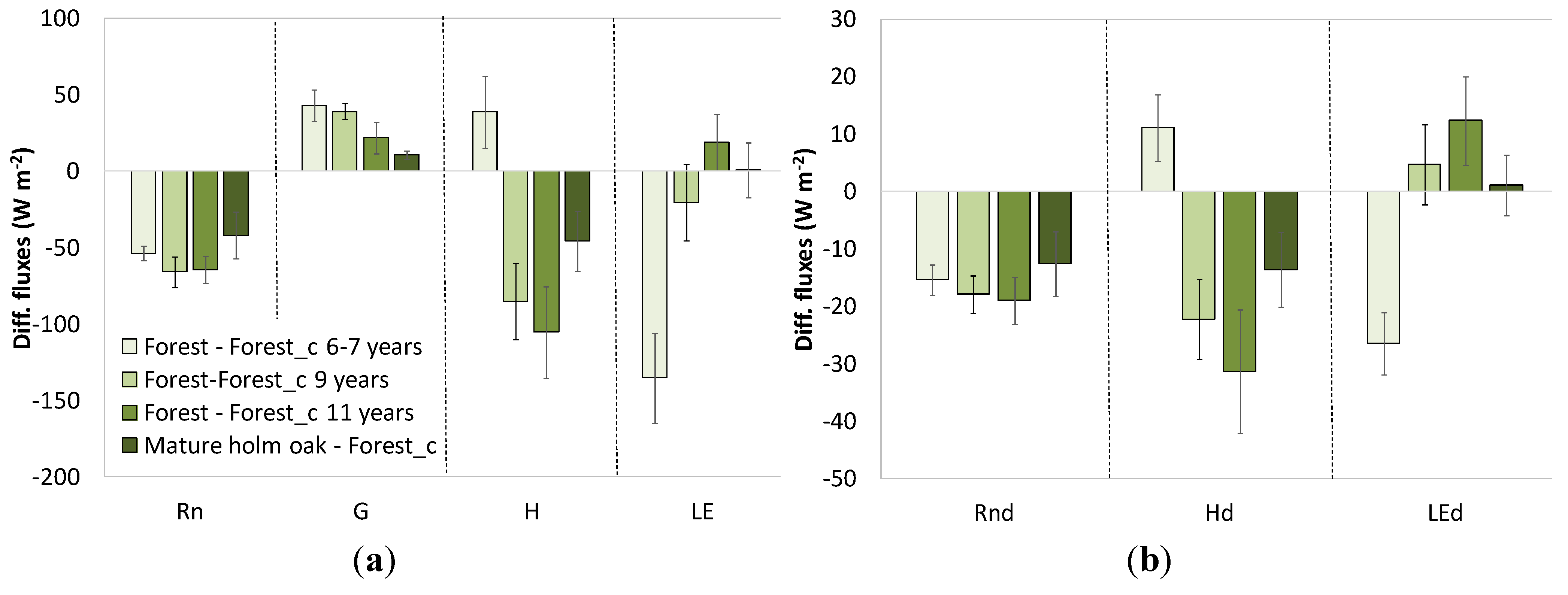
3.3.2. Effects on Energy Fluxes in the Forest Site

Figure 6 shows the plots of the differences in terms of surface energy fluxes between estimated values for both the forest and shrub areas and their respective control sites. The increase in albedo and TR in the forest area produces a decrease in both shortwave and longwave net radiation, yielding an average net decrease in Rni of 54 ± 5 W·m−2 after six years, 66 ± 10 W·m−2 after nine years, and 64 ± 9 W·m−2 after 11 years. The opposite effect is observed in Gi, with an average increase of 43 ± 10 W·m−2, 39 ± 5 W·m−2, and 22 ± 10 W·m−2 after six, seven, nine, and 11 years, respectively. At a daily scale the average decrease in Rnd results in 15 ± 3 W·m−2, 18 ± 3 W·m−2, and 19 ± 4 W·m−2. Note that differences between these three periods are not statistically significant in terms of Rn and G.
Figure 6. Average values of the differences between burnt and unburnt areas in terms of Rn, G, H, and LE: (a) instantaneous fluxes; (b) daily fluxes. Error bars represent the standard deviations of the averages.
Remotesensing 07 14899 g006
A decrease in Pv yields higher H in the burnt area after 6–7 years, in average 40 ± 20 W·m−2 at the time of the satellite overpass, and 11 ± 6 W·m−2 at daily scale. As a result, LE is lower, 140 ± 30 W·m−2 at the instantaneous scale, and 27 ± 5 W·m−2 (~1 mm·day−1) at the daily scale. This trend changes after nine years, most likely guided by the change in vegetation structure (see Figure 1b) in combination with the evolution in Pv. Sensible heat flux decreases after nine years in the burnt area showing differences with the control site of −85 ± 25 W·m−2 at the instantaneous scale, and −22 ± 13 W·m−2 at the daily scale. These differences remain after 11 years, with instantaneous values of −110 ± 30 W·m−2 at, and −31 ± 11 W·m−2 at daily scale. Differences in LE are not statistically significant in the forest area after nine years, −20 ± 25 W·m−2 and 5 ± 13 W·m−2 at instantaneous and daily scales, respectively. Very similar values are observed after 11 years, with differences in LE of 19 ± 19 W·m−2 and 12 ± 8 W·m−2 at instantaneous and daily scales, respectively.

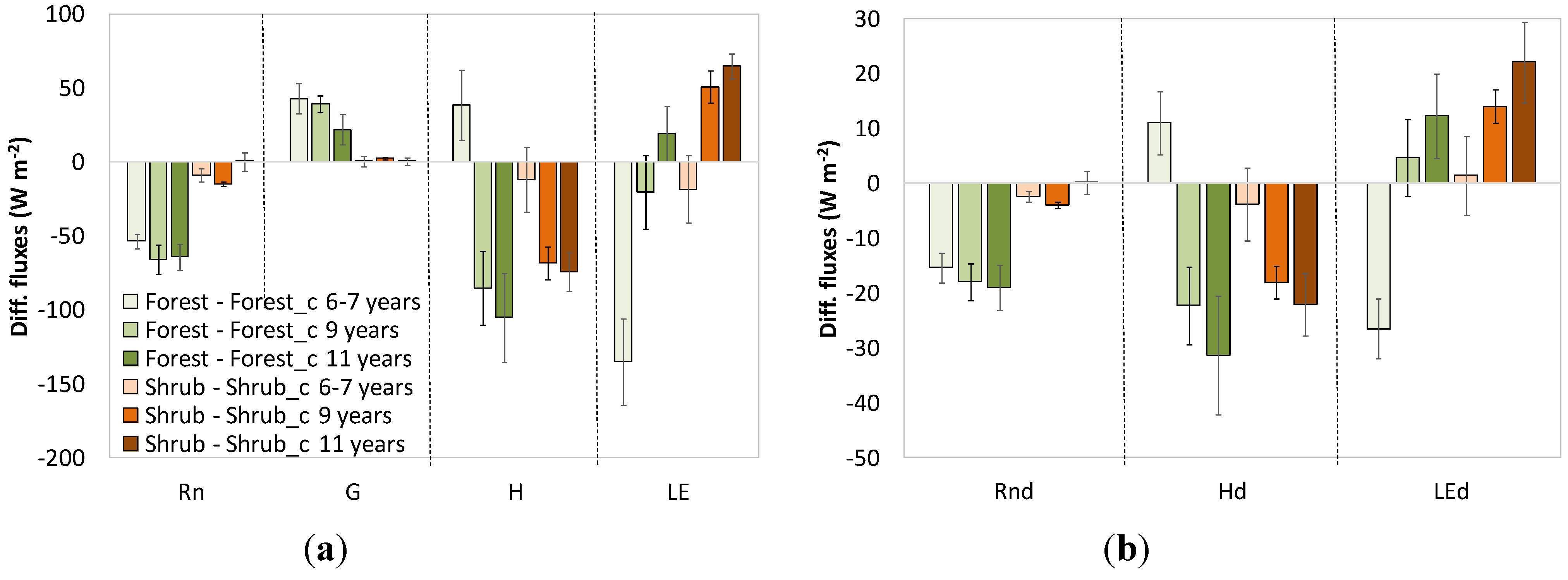
3.3.3. Effects on Energy Fluxes in the Shrub Site

Focusing now on the shrubs site, very minor changes in the flux patterns are observed 6–7 years after the fire. This is in agreement with the negligible variations in albedo, NDVI, Pv, and TR shown above (Figure 5) for this period. However, an important decrease in H (−69 ± 11 W·m−2), and consequent increase in LE (51 ± 11 W·m−2), is observed after nine years. These differences stay very similar 11 years after the fire. These variations might be produced by changes in the canopy structure of the area (see Figure 1). Daily LE increases as much as 22 ± 7 W·m−2 (~0.8 mm·day−1) after 11 years.

3.3.4. Effects on Energy Fluxes in the Future Scenario

Figure 7 shows the effect of the fire in a future scenario in which the burnt area has been naturally reforested and a mature Holm oak forest is occupying the area. With this aim, differences between the forest_c area and a selected area representative of the mature holm oak forest (Figure 1c) are shown. Note that Rn remains very similar for the two forest types. However, compared to the period of 11 years after the fire event, differences in terms of G and H would be halved, at both instantaneous and daily scales. The effect in terms of LE is shown almost null for the future scenario, as a result of the similar reduction in both H and Rn. We might then conclude that the land cover change from pine to Holm oak does not have a significant long-term effect on the evapotranspiration, whereas net radiation and sensible heat flux will decrease in a similar quantity.
Comparison with earlier literature is not easy due to the differences in the land covers burnt and the variety in land cover changes. Montes-Helu et al. [5] analyzed the change on energy fluxes 10 years after a fire event in a forest area naturally revegetated by grassland. In agreement with our findings, these authors observed an increased albedo resulting in a decrease of Rn. The seasonal analysis in [5] showed greater LE at the unburnt site between April and October. This is also in agreement with our results 6–7 years after the fire, but not so evident after nine or 11 years. Rocha et al. [6] studied the change on surface energy exchange and temperature in a burnt arctic tundra area along the three years following the fire event, attending to different burn severity gradients (severe and moderate). They observed a decreased albedo in the first two years after the fire event, the third year the albedo of the severely burnt and the unburnt areas were close, while in the moderately burnt area, the albedo was higher than in the unburnt area. Latent heat fluxes were also higher in burnt area, while sensible heat flux of burnt and unburnt areas were similar during the first two years, and in the third year it was lower in the burnt area.
Figure 7. Average values of the differences between burnt and unburnt forest, and between forest and mature holm oak areas, in terms of Rn, G, H, and LE: (a) Instantaneous fluxes; (b) Daily fluxes. Error bars represent the standard deviations of the averages.
Remotesensing 07 14899 g007
Most of the works in the literature dealing with similar analysis are based on ground measurements. However, these local measures show temporal and spatial limitations. Remote sensing allows the continuous monitoring of energy fluxes, covering large areas. Moreover, the vast Landsat archive allows these kinds of studies longer than 40 years back in time, which provides a unique opportunity to analyze the time evolution of the effect of fires on the surface energy fluxes.

4. Conclusions

An analysis of changes in surface energy fluxes after a fire event is conducted using remote sensing data. This forest fire occurred in a Mediterranean pine and shrub area. The burnt area was naturally reforested. Landsat TM and ETM+ imagery was used to retrieve the surface parameters required in the STSEB model to monitor the different terms of the energy balance equation. The comparison of the energy fluxes between the burnt site and three unburnt control sites (forest, shrubland and mature holm oak) showed that the shrub area regenerates after 6–7 years of the fire event; similar fluxes compared to the shrub control site were observed. In the forest area, the increased albedo and temperature, together with the decreased vegetation cover fraction, yield a drop in net radiation (54 ± 5 W·m−2), a rise in ground (43 ± 10 W·m−2) and sensible heat (40 ± 20 W·m−2) fluxes, and an important drop in latent heat flux (−140 ± 30 W·m−2), at an instantaneous scale after 6–7 years of the fire event. At a daily scale this implies a reduction in evapotranspiration around 1 mm·day−1. This trends change after nine years, and differences in sensible heat flux turn negative, resulting in a non-significant increase in latent heat flux. A future scenario is analyzed by comparison with an area of mature holm oak. Differences in surface energy fluxes diminish and, based on these findings, no significant long-term effect is expected on the evapotranspiration of a Mediterranean pine forest burnt and naturally reforested.
This paper shows the potential of remote sensing techniques to analyze the effects of present and past land cover changes on the surface energy flux patterns, beyond the limited local information provided by ground measurements.

Acknowledgments

This work was supported by the Spanish Ministry of Economy and Competitiveness (project CGL2013-46862-C2-1/2-P, co-financed with European Union FEDER funds, and AGL2014-55658-R), Generalitat Valenciana (project PROMETEOII/2014/086) and the JCCM (project ECOFLUX III, Ref: PEIC-2014-002-P).

Author Contributions

Juan M. Sánchez as the main author developed and implemented the approach. Mar Bisquert helped in the data analysis and preparation of figures and tables. Eva Rubio was responsible of the validation data acquisition. Vicente Caselles proposed the study and cross-checked the manuscript.

Conflicts of Interest

The authors declare no conflict of interest.

References

  1. Clark, K.L.; Skowronski, N.; Gallagher, M.; Renninger, H.; Schäfer, K. Effects of invasive insects and fire on forest energy exchange and evapotranspiration in the New Jersey pinelands. For. Meteorol. 2012, 166, 50–61. [Google Scholar] [CrossRef]
  2. Randerson, J.T.; Liu, H.; Flanner, M.G.; Chambers, S.D.; Jin, Y.; Hess, P.G.; Pfister, G.; Mack, M.C.; Treseder, K.K.; Welp, L.R.; et al. The impact of boreal forest fire on climate warming. Science 2006, 314, 1130–1132. [Google Scholar] [CrossRef] [PubMed]
  3. Amiro, B.D.; Orchansky, A.L.; Barr, A.G.; Black, T.A.; Chambers, S.D.; Chapin, F.S., III; Goulden, M.L.; Litvak, M.; Liu, H.P.; McCaughey, J.H.; et al. The effect of post-fire stand age on the boreal forest energy balance. Agric. For. Meteorol. 2006, 140, 41–50. [Google Scholar] [CrossRef]
  4. Dore, S.; Kolb, T.E.; Montes-Helu, M.; Eckert, S.E.; Sullivan, B.W.; Hungate, B.A.; Kaye, J.P.; Hart, S.C.; Koch, G.W.; Finkral, A. Carbon and water fluxes from ponderosa pine forests disturbed by wildfire and thinning. Ecol. Appl. 2010, 20, 663–683. [Google Scholar] [CrossRef] [PubMed]
  5. Montes-Helu, M.C.; Kolb, T.; Dore, S.; Sullivan, B.; Hart, S.C.; Koch, G.; Hungate, B.A. Persistent effects of fire-induced vegetation change on energy partitioning and evapotranspiration in ponderosa pine forests. Agric. For. Meteorol. 2009, 149, 491–500. [Google Scholar] [CrossRef]
  6. Rocha, A.V.; Shaver, G.R. Postfire energy exchange in arctic tundra: The importance and climatic implications of burn severity. Glob. Chang. Biol. 2011, 17, 2831–2841. [Google Scholar] [CrossRef]
  7. Lentile, L.B.; Holden, Z.A.; Smith, A.M.S.; Falkowski, M.J.; Hudak, A.T.; Morgan, P.; Lewis, S.A.; Gessler, P.E.; Benson, N.C. Remote sensing techniques to assess active fire characteristics andpost-fire effects. Int. J. Wildland Fire 2006, 15, 319–345. [Google Scholar] [CrossRef]
  8. López, M.J.; Caselles, V. Mapping burns and natural reforestation using thematic mapper data. Gocarto. Int. 1991, 1, 31–37. [Google Scholar]
  9. Díaz-Delgado, R.; Lloret, F.; Pons, X. Influence of fire severity on plant regeneration by means of remote sensing imagery. Int. J. Remote Sens. 2003, 8, 1751–1763. [Google Scholar] [CrossRef]
  10. Ha, W.; Kolb, T.E.; Springer, A.E.; Dore, S.; O′Donnell, F.C.; Martínez, R.; López, S.; Koch, G.W. Evapotranspiration comparisons between eddy covariance measurements and meteorological and remote-sensing-based models in disturbed ponderosa pine forests. Ecohydrology 2014, 8, 1335. [Google Scholar] [CrossRef]
  11. Wang, J.; Sammis, T.W.; Meier, C.A.; Simmons, L.J.; Miller, D.R.; Bathke, D. Remote sensing vegetation recovery after forest fires using energy balance. In Proceedings of the Sixth Symposium on Fire and Forest Meteorology, Canmore, AB, Canada, 25–27 October 2005; p. 76.
  12. Monteith, J.L.; Unsworth, M.H. Principles of Environmental Physics, 4rd ed.; Academic Press: Boston, MA, USA, 2013; p. 241. [Google Scholar]
  13. Hall, F.G.; Huemmrich, K.F.; Goetz, S.J.; Sellers, P.J.; Nickeson, J.E. Satellite remote sensing of surface energy balance: Success, failures, and unresolved issues in FIFE. J. Geophys. Res. 1992, 97, 19061–19089. [Google Scholar] [CrossRef]
  14. Shuttleworth, W.J.; Wallace, J.S. Evaporation from sparse crops-an energy combination theory. Q. J. R. Meteorol. Soc. 1985, 111, 839–855. [Google Scholar] [CrossRef]
  15. Choudhury, B.J.; Idso, S.B.; Reginato, R.J. Analysis of an empirical model for soil heat flux under a growing wheat crop for estimating evaporation by an infrared-temperature based energy balance equation. Agric. For. Meteorol. 1987, 39, 283–297. [Google Scholar] [CrossRef]
  16. Norman, J.M.; Kustas, W.; Humes, K. A two-source approach for estimating soil and vegetation energy fluxes from observations of directional radiometric surface temperature. Agric. For. Meteorol. 1995, 77, 263–293. [Google Scholar] [CrossRef]
  17. Sánchez, J.M.; Kustas, W.P.; Caselles, V.; Anderson, M.C. Modelling surface energy fluxes over maize using a two-source patch model and radiometric soil and canopy temperature observations. Remote Sens. Environ. 2008, 112, 1130–1143. [Google Scholar] [CrossRef]
  18. Sánchez, J.M.; Caselles, V.; Niclòs, R.; Coll, C.; Kustas, W.P. Estimating energy balance fluxes above a boreal forest from radiometric temperature observations. Agric. For. Meteorol. 2009, 149, 1037–1049. [Google Scholar] [CrossRef]
  19. Sánchez, J.M.; Scavone, G.; Caselles, V.; Valor, E.; Copertino, V.A.; Telesca, V. Monitoring daily evapotranspiration at a regional scale from Landsat-TM and ETM+ data: Application to the Basilicata region. J. Hydrol. 2008, 351, 58–70. [Google Scholar] [CrossRef]
  20. López Serrano, F.R.; de las Heras, J.; Moya, D.; García-Morote, A.; Rubio, E. Is the net primary productivity of a coppice forest stand of quercus ilex affected by post-fire thinning treatments and by recurrent fires? Int. J. Wildland Fire 2010, 19, 637–648. [Google Scholar] [CrossRef]
  21. Lamont, B.B.; Le Maitre, D.C.; Cowling, R.M.; Enright, N.J. Canopy seed storage in woody plants. Bot. Rev. 1991, 57, 277–317. [Google Scholar] [CrossRef]
  22. Corine Land Cover; Technical Guidelines; EEA Press: Copenhagen, Denmark, 2007; p. 70.
  23. Earth Explorer. Available online: https://earthexplorer.usgs.gov (accessed on 1 July 2015).
  24. Barsi, J.A.; Barker, J.L.; Schott, J.R. An atmospheric correction parameter calculator for a single thermal band earth-sensing instrument. In Proceedings of Geoscience and Remote Sensing Symposium, Toulouse, France, 21–25 July 2003; Volume 5, pp. 3014–3016.
  25. Barsi, J.A.; Schott, J.R.; Palluconi, F.D.; Hook, S.J. Validation of a web-based atmospheric correction tool for single thermal band instruments. SPIE 2005, 5882, 58820E-1–58820E-7. [Google Scholar]
  26. Dubayah, R. Estimating net solar radiation using Landsat Thematic Mapper and digital elevation data. Water Resour. Res. 1992, 28, 2469–2484. [Google Scholar] [CrossRef]
  27. Valor, E.; Caselles, V. Validation of the vegetation cover method for land surface emissivity estimation. In Recent Research Developments in Thermal Remote Sensing; Research Signpost: Kerala, India, 2005; pp. 1–20. [Google Scholar]
  28. Valor, E.; Caselles, V. Mapping land surface emissivity from NDVI: Application to European, African, and South American areas. Remote Sens. Environ. 1996, 57, 167–184. [Google Scholar] [CrossRef]
  29. Humes, K.S.; Kustas, W.P.; Moran, M.S. Use of remote sensing and reference site measurements to estimate instantaneous surface energy balance components over a semiarid rangeland watershed. Water Resour. Res. 1994, 30, 1363–1373. [Google Scholar] [CrossRef]
  30. Kustas, W.P.; Goodrich, D.C. Preface. Water Resour. Res. 1994, 30, 1211–1225. [Google Scholar] [CrossRef]
  31. Seguin, B.; Itier, B. Using midday surface temperature to estimate daily evaporation from satellite thermal IR data. Int. J. Remote Sens. 1983, 4, 371–383. [Google Scholar] [CrossRef]
  32. Lagouarde, J.-P.; McAneney, K.J. Daily sensible heat flux estimation from a single measurement of surface temperature and maximum air temperature. Bound.-Layer Meteorol. 1992, 59, 341–362. [Google Scholar] [CrossRef]
  33. Sánchez, J.M.; Caselles, V.; Niclòs, R.; Valor, E.; Coll, C.; Laurila, T. Evaluation of the B-method for determining actual evapotranspiration in a boreal forest from MODIS data. Int. J. Remote Sens. 2007, 28, 1231–1250. [Google Scholar] [CrossRef]

