Weighted-Fusion-Based Representation Classifiers for Hyperspectral Imagery

Abstract

Spatial texture features have been demonstrated to be very useful for the recently-proposed representation-based classifiers, such as the sparse representation-based classifier (SRC) and nearest regularized subspace (NRS). In this work, a weighted residual-fusion-based strategy with multiple features is proposed for these classifiers. Multiple features include local binary patterns (LBP), Gabor features, and the original spectral signatures. In the proposed classification framework, representation residuals for a testing pixel from using each type of features are weighted to generate the final representation residual, and then the label of the testing pixel is determined according to the class yielding the minimum final residual. The motivation of this work is that different features represent pixels from different perspectives and their fusion in the residual domain can enhance the discriminative ability. Experimental results of several real hyperspectral image datasets demonstrate that the proposed residual-based fusion outperforms the original NRS, SRC, support vector machine (SVM) with LBP, and SVM with Gabor features, even in small-sample-size (SSS) situations.

1. Introduction

Containing hundreds of spectral narrow bands, hyperspectral imagery has a very high spectral resolution that provides potential for more accurate object classification. Numerous classification algorithms [1,2] using hyperspectral data have been developed for a variety of applications, such as mineral exploration, environmental monitoring, etc. With the advance of sensor technology, hyperspectral images with high spatial resolution are becoming more available.

Recently, representation-based classification, which does not assume any data density distribution, has attracted great interest. In our previous work, nearest regularized subspace (NRS) [3] was proposed for hyperspectral image classification, where each testing pixel was represented by a linear combination of all available labeled samples per class and the class label was the one whose training samples provide the lowest representation residual. Moreover, a distance-weighted Tikhonov regularization was employed to impose adaptive penalty on representation coefficients of different training samples in the way that samples more similar to the testing pixel could be assigned with larger coefficients. The NRS has a closed-form solution, and has been demonstrated to be more efficient than the state-of-the-art classifiers, such as support vector machine (SVM) [2].

Sparse representation-based classification (SRC) [4] was originally introduced in computer vision [5,6], and first applied to hyperspectral image classification in [7]. Tang et al. [8] proposed a classifier based on the SRC, which outperformed some popular classification methods, such as the SVM, subspace projection (SP), orthogonal matching pursuit (OMP), and so on. Similar to the NRS, the SRC determines the class label of a testing pixel by solving a problem of sparse regression between training samples and a testing pixel. However, the solution of sparse coefficients may not be unique or stable when the atoms in a dictionary contain high mutual coherence [9,10]. In order to alleviate such problems, improvement strategies have been applied on the SRC with structured priors, including joint sparsity (JS) [11], low-rank (LR) Lasso [12], collaborative hierarchical Lasso (CHiLasso) [13], and so on.

With the improvement of spatial resolution, spatial information has been utilized for hyperspectral image classification [14,15,16,17,18,19]. For example, composite kernels (CK) for both spectral and spatial features were employed by a SVM classifier, referred to as SVM-CK [14]. Recently, spatial features, such as morphological attribute profile (MAP) [15,20,21], 2-D Gabor features [16,22], 3-D Gabor features [17], gray level co-occurrence matrix (GLCM) [18], local binary patterns (LBP) [19], and shape features [23], were investigated, and a number of spatial features were combined for the representation-based classifiers. In [16], the benefits of using spatial features extracted from a Gabor filter for the NRS were demonstrated. In [24], weighted joint collaborative representation (WJCR) classification was investigated. For face recognition, Lee et al. [25] introduced a robust method that applied the Gabor-edge components histogram on the SRC. A joint sparse representation model (JSRM) was proposed in [26,27,28]. Multiscale adaptive sparse representation was developed to reduce the sensitivity to region size in the JSRM [29].

Along with algorithm development for hyperspectral image classification, feature-level and decision-level fusion have been investigated [23,30,31]. Waske et al. [30] analyzed the robustness of multiple classifier systems based on the SVM and random feature selection, and it was demonstrated that the combination of the selected features for multiple classifiers could truly improve classification accuracy. In [31], an adaptive affinity propagation algorithm was proposed for dimension reduction for classification improvement. In [32,33], novel frameworks by combining supervised and unsupervised learning methods (e.g., SVM and fuzzy-c-means clustering algorithm) were developed. Decision fusion could also improve the performance of target and anomaly detection [34]. In [35], a wavelet-based NRS classifier for noise-robust hyperspectral image classification based on redundant discrete wavelet transformation was introduced. In [36], a dynamic classifier selection approach was presented, where both spatial and spectral information were used to determine the label of a testing pixel once the remaining neighborhood meets the threshold.

In this paper, a weighted-residual-fusion-based strategy with multiple features is proposed for representation-based classifiers. Multiple features include LBP features, Gabor features, and the original spectral signatures. In the proposed classification framework, each type of feature is used for the NRS or SRC, generating multiple representation residuals, and then all these residuals are added together with different weights [37] and the label of the testing pixel is determined according to the class yielding the minimum weighted sum of the residuals. The LBP and Gabor feature are employed due to the facts that the LBP has an excellent ability to describe local image texture features and a Gabor filter is able to extract global features. It is expected that different types of spatial features reflect the characteristics of a pixel from different perspectives and their fusion in the residual domain is able to enhance class separability even in small-sample-size (SSS) situations.

2. Proposed Classification Framework

2.1. Gabor-Filter

A Gabor filter [38] is an orientation-dependent band-pass filter with orientation sensitive but rotation invariant characteristics. Here, Gabor features are the magnitudes of each Gabor-filtered image, which is equivalent to signal power in the corresponding filter pass band. In a 2-D (a, b) coordinate system, a Gabor filter, including a real and imaginary term, is represented as,

$$G_{\delta ,\theta ,\varphi ,\sigma \sigma }\left(a,b\right)=\text{exp}\left(-\frac{{a^{\prime }}^2+{\gamma }^2{b^{\prime }}^2}{2{\sigma }^2}\right)\text{exp}\left(j\left(2\pi \frac{a^{\prime }}{\delta }+\varphi \right)\right)$$

(1)

where:

$$a^{\prime }=a\text{cos}\theta +b\text{sin}\theta$$

(2)

$$b^{\prime }=-a\text{sin}\theta +b\text{cos}\theta$$

(3)

In Equation (1), δ is the wavelength of the sinusoidal factor, θ is the orientation separation angle (e.g., $\frac{\pi }{8}，\frac{\pi }{4}，\frac{\pi }{2}，$ etc.) of Gabor kernels, φ represents the phase offset, σ is the standard derivation of the Gaussian envelope, and γ is the spatial aspects ratio specifying the ellipticity of the support of the Gabor function. ϕ = 0 and $\varphi =\frac{\pi }{2}$ return the real and imaginary parts of the Gabor filter, respectively. Parameter σ is determined by δ and spatial frequency bandwidth bw as,

$$\sigma =\frac{\delta }{\pi }\sqrt{\frac{\text{ln}2}{2}}\frac{2^{bw}+1}{2^{bw}-1}$$

(4)

2.2. LBP

Recently, the original LBP [39] and its variants have been used to extract rotation invariant features for classification. An entire image is convoluted by a small mask, e.g., a 3 × 3 window; for each central pixel in the window, its gray value is compared with its surrounding 8 pixels; a binary label is then obtained, which can be either “0” or “1” (0 means a smaller gray value and 1 means a larger one). For a general case, let m represent the number of surrounding neighbors and let these pixels be denoted as ${\left\{g_i\right\}}_{i=0}^{m-1}$. For the center pixel g_c, its LBP code is calculated as,

$$LB{P}_{m,r}\left(g_c\right)={\displaystyle \sum _{i=0}^{m-1}}U\left(g_i-g_c\right)2^i$$

(5)

where the function U(.) is defined as

$$U\left(g\right)=\{\begin{array}{l}1,g_i\ge g_c\\ 0,g_i<g_c\end{array}$$

(6)

As illustrated in Figure 1, for each pixel, a binary number is obtained by concatenating all these binary values in a clockwise direction, which starts from one of its top-middle neighbors. It is easy to observe that such an LBP operator actually represents the texture orientation and smoothness information in a local region. For a 3 × 3 mask, the eight labels compose the center pixel’s binary numbers that can be further converted into decimal numbers as an LBP code. Then, an occurrence histogram, as a nonparametric statistical estimate, is calculated; during the process, a binning procedure is required to ensure that the extracted histogram features have the same dimensions. Furthermore, to deal with textures at different scales, the LBP operator may use windows of different sizes [39]. The original rotation invariant LBP is achieved by circularly rotating each bit pattern to the minimum value. In our work, a variant of LBP called “uniform-LBP” is employed, where the histogram has a separate bin for every uniform pattern, while all non-uniform patterns are assigned to a single bin. Here, a pattern is called uniform if the binary pattern contains at most two circular 0–1 and 1–0 transitions. Selecting uniform patterns appropriately can reduce the length of the feature vector, thereby improving classification performance [19,40,41].

Figure 1. An example of LBP binary thresholding: (a) a 3 × 3 window; and (b) binary labels of the surrounding eight neighbors (in the clockwise direction).

Figure 1. An example of LBP binary thresholding: (a) a 3 × 3 window; and (b) binary labels of the surrounding eight neighbors (in the clockwise direction).

2.3. NRS

Consider a dataset with training samples $\mathbf{X}={\left\{{\mathbf{x}}_i\right\}}_{i=1}^n$ in a d-dimensionality space with class labels being denoted as ${\mathbf{Q}}_i\in \left\{1,2,\dots ,C\right\}$, where C is the number of classes, n is the total number of training samples. Let the number of training samples in the l-th class be represented as n_l. In the NRS, y_l represents the class-specific approximation in the l-th class of a test pixel y, which is calculated via a linear combination of available training samples in the l-th class X_l, with the weight factor α_l as,

$${\mathbf{y}}_l={\mathbf{X}}_l\cdot {\mathbf{\text{α}}}_l$$

(7)

The optimal α_l can be solved by an ℓ₂−norm regularization described as,

$${\mathbf{\text{α}}}_l=\text{arg}\underset{{\mathbf{\text{α}}}_l^{\ast }}{\text{min}}{\Vert \mathbf{y}-{\mathbf{X}}_l{\mathbf{\text{α}}}_l^{\ast }\Vert }_2^2+\lambda {\Vert {\mathbf{\Gamma }}_{l,y}{\mathbf{\text{α}}}_l^{\ast }\Vert }_2^2$$

(8)

where λ is a regularization parameter , and the biasing Tikhonov matrix defined as,

$${\mathbf{\Gamma }}_{l,y}=\left[\begin{array}{ccc}{\Vert \mathbf{y}-{\mathbf{x}}_{l,1}\Vert }_2& \cdots & 0\\ ⋮& \ddots & ⋮\\ 0& \dots & {\Vert \mathbf{y}-{\mathbf{x}}_{l,n_l}\Vert }_2\end{array}\right]$$

(9)

which can reflect the data locality structure in the calculated weight coefficients; that is, the labeled samples that are most dissimilar to the testing pixel will provide a much smaller contribution to the linear representation. A closed-form solution of the weight vector α_l in Equation (8) can be directly calculated as,

$${\mathbf{\text{α}}}_l={\left({\mathbf{X}}_l^T{\mathbf{X}}_l+{\lambda }^2{\mathbf{\Gamma }}_{l,y}^T{\mathbf{\Gamma }}_{l,y}\right)}^{-1}{\mathbf{X}}_l^T\mathbf{y}$$

(10)

After the weight vector is obtained, the class label of the testing pixel is determined according to the class that minimizes the Euclidean distance between y_l and y, i.e.,

$${\mathbf{r}}_l(\mathbf{y})={\Vert {\mathbf{y}}_l-\mathbf{y}\Vert }_2={\Vert {\mathbf{X}}_l{\mathbf{\text{α}}}_l-\mathbf{y}\Vert }_2$$

(11)

and class

$$(\mathbf{y})=\text{arg}{\text{min}}_{l=1,\dots ,C}{\mathbf{r}}_l(\mathbf{y})$$

2.4. SRC

The basic idea of SRC is to represent the testing pixel y as a sparse linear combination of a training sample dictionary X containing samples from all the C classes. Then, the sparse representation coefficients $\mathbf{\text{α}}=[{\mathbf{\text{α}}}_{\mathbf{1}},{\mathbf{\text{α}}}_{\mathbf{i}},\dots ,{\mathbf{\text{α}}}_{\mathbf{c}}]$ can be estimated by solving the following l₁ minimization problem:

$$\widehat{\alpha }=\text{arg}\underset{\alpha }{\text{min}}{\Vert \mathbf{y}-\mathbf{X}\mathbf{\text{α}}\Vert }_2^2+\lambda {\Vert \mathbf{\text{α}}\Vert }_1$$

(12)

In our work, the l₁-norm minimization is solved using the l1_ls package (SRC with the l₁-norm minimization is implemented using the l1_ls package [42]. Then, similarly, the label of the testing pixel is determined by computing the representation residual per class.

2.5. Residual-Fusion-Based-Collaborative Representation

Figure 2 illustrates the flowchart of the proposed weighted-residual-fusion-based classifier (NRC or SRC) that merges three representation residuals from using three types of features (i.e., LBP features, Gabor features, and the original spectral features). During the feature exaction process, band-selection-based dimensionality reduction is conducted with the linear prediction error (LPE) criterion [43,44], which is an unsupervised band selection method to find a small set of distinctive and informative bands. Based on the concept that a band yielding the maximum reconstruction error is considered as the most dissimilar band, LPE begins with the best two-band combination, and then augments this two-band combination to three, four, and so on, until a desired number of bands is selected. For each selected band, the LBP operator and the Gabor filter are used to extract spatial features as described previously. As shown in Equation (11), each NRS and SRC classifier (before assigning class membership) produces a certain representation residual. The residuals from using different types of features are combined to generate a weighted sum as

$$\begin{array}{l}{\mathbf{r}}_l(\mathbf{y})=w_1{\mathbf{r}}_l^S(\mathbf{y})+w_2{\mathbf{r}}_l^L(\mathbf{y})+w_3{\mathbf{r}}_l^G(\mathbf{y})\\ \text{s.t.} w_1+w_2+w_3=1, w_1\ge 0 w_2\ge 0,w_3\ge 0\end{array}$$

(13)

where ${\mathbf{r}}_l^S(\mathbf{y})$, ${\mathbf{r}}_l^L(\mathbf{y})$ and ${\mathbf{r}}_l^G(\mathbf{y})$ are the residuals when using the l-th class’ labeled samples with the original spectral features (the resulting classifiers are denoted as Spec-NRS for NRS or Spec-SRC for SRC), the LBP features (denoted as LBP-NRS or LBP-SRC), and with Gabor features (denoted as Gabor-NRS or Gabor-SRC), respectively. The class label of the testing pixel y is determined by the one producing the minimum weighted sum of residual. Here, w₁, w₂, and w₃ are the weights of residuals when using the spectral signatures, LBP features, and Gabor features, respectively. A larger weight means the corresponding feature is more important in decision making, which is obviously data and class dependent. Note that these weights are imposed with non-negativity and sum-to-one constraints.

Figure 2. Flowchart of the proposed residual-fusion-based strategy with multiple features and representation-based classifiers.

Figure 2. Flowchart of the proposed residual-fusion-based strategy with multiple features and representation-based classifiers.

In the proposed weighted-residual-fusion-based classifier, both LBP and Gabor features are extracted to present spatial information. Note that Gabor features are produced by the average magnitude response for each Gabor filtered image reflecting the global signal power, while the LBP-coded image is an expression of detailed local spatial features, such as edges, corners, and knots. Thus, Gabor filtering is a supplement to the local LBP that lacks the consideration of distant pixel interactions. It is expected that different features represent a testing pixel from different perspectives, and fusion of these features can enhance discriminative power.

3. Experimental Section

In this section, the performance of the proposed weighted-residual-fusion-based representation classifiers, denoted as RF-NRS and RF-SRC, on two real hyperspectral datasets is investigated. The classification results are compared with other algorithms, such as the original NRS or SRC using spectral signatures only, LBP-NRS or LBP-SRC using LBP features only, Gabor-NRS or Gabor-SRC using Gabor features only, and SVM using Gabor-filtering and LBP features. All experimental data are downloaded from a public website [45].

The first experimental data were collected by the Reflective Optics System Imaging Spectrometer (ROSIS) sensor [46]. The image scene, with a spatial size of 610 × 340 pixels, covers the city of Pavia, Italy. The data set has 91 spectral bands after water-band removal. It has a spectral coverage from 0.43–0.86 um and a spatial resolution of 1.3 m. There are nine classes from the ground truth map.

The second data were collected by the AVIRIS sensor over an area in Salinas Valley, California with a spatial resolution of 3.7 m. The image comprises 512 × 217 pixels with 204 bands (after 20 water absorption bands are removed). It mainly contains vegetables, bar soils, and vineyard fields. There are 16 classes from the ground truth map. With the same sensor, another scene was collected over northwest Indiana’s Indian Pine test site in 1992. The scene consists of 145 × 145 pixels with a spatial resolution of 20 m. There are also 16 different land-cover classes.

Table 1. Labeled samples for the University of Pavia dataset.

Class		Number of Samples
NO.	Name
1	Asphalt	6631
2	Meadows	18,649
3	Gravel	2099
4	Trees	3064
5	Painted metal sheets	1345
6	Bare soil	5029
7	Bitumen	1330
8	Self-blocking bricks	3682
9	Shadows	947
Total		42,776

Table 1. Labeled samples for the University of Pavia dataset.

Class		Number of Samples
NO.	Name
1	Asphalt	6631
2	Meadows	18,649
3	Gravel	2099
4	Trees	3064
5	Painted metal sheets	1345
6	Bare soil	5029
7	Bitumen	1330
8	Self-blocking bricks	3682
9	Shadows	947
Total		42,776

The information of classes and their labeled samples for both the Salinas and University of Pavia datasets are given in Table 1 and Table 2. All experiments are carried out using MATLAB on an Intel i7 quad core 3.40-GHz machine with 10 GB of RAM.

Table 2. Labeled samples for the Salinas dataset.

Class		Number of Samples
NO.	Name
1	Brocoli_green_weeds_1	2009
2	Brocoli_green_weeds_2	3726
3	Fallow	1976
4	Fallow_rough_plow	1394
5	Fallow_smooth	2678
6	Stubble	3959
7	Celery	3579
8	Grapes_untrained	11,271
9	Soil_vinyard_develop	6203
10	Corn_senesced_green_weeds	3278
11	Lettuce_romaine_4wk	1068
12	Lettuce_romaine_5wk	1927
13	Lettuce_romaine_6wk	916
14	Lettuce_romaine_7wk	1070
15	Vinyard_untrained	7268
16	Vinyard_vertical_trellis	1807
Total		50,550

Table 2. Labeled samples for the Salinas dataset.

Class		Number of Samples
NO.	Name
1	Brocoli_green_weeds_1	2009
2	Brocoli_green_weeds_2	3726
3	Fallow	1976
4	Fallow_rough_plow	1394
5	Fallow_smooth	2678
6	Stubble	3959
7	Celery	3579
8	Grapes_untrained	11,271
9	Soil_vinyard_develop	6203
10	Corn_senesced_green_weeds	3278
11	Lettuce_romaine_4wk	1068
12	Lettuce_romaine_5wk	1927
13	Lettuce_romaine_6wk	916
14	Lettuce_romaine_7wk	1070
15	Vinyard_untrained	7268
16	Vinyard_vertical_trellis	1807
Total		50,550

3.1. Parameter Tuning

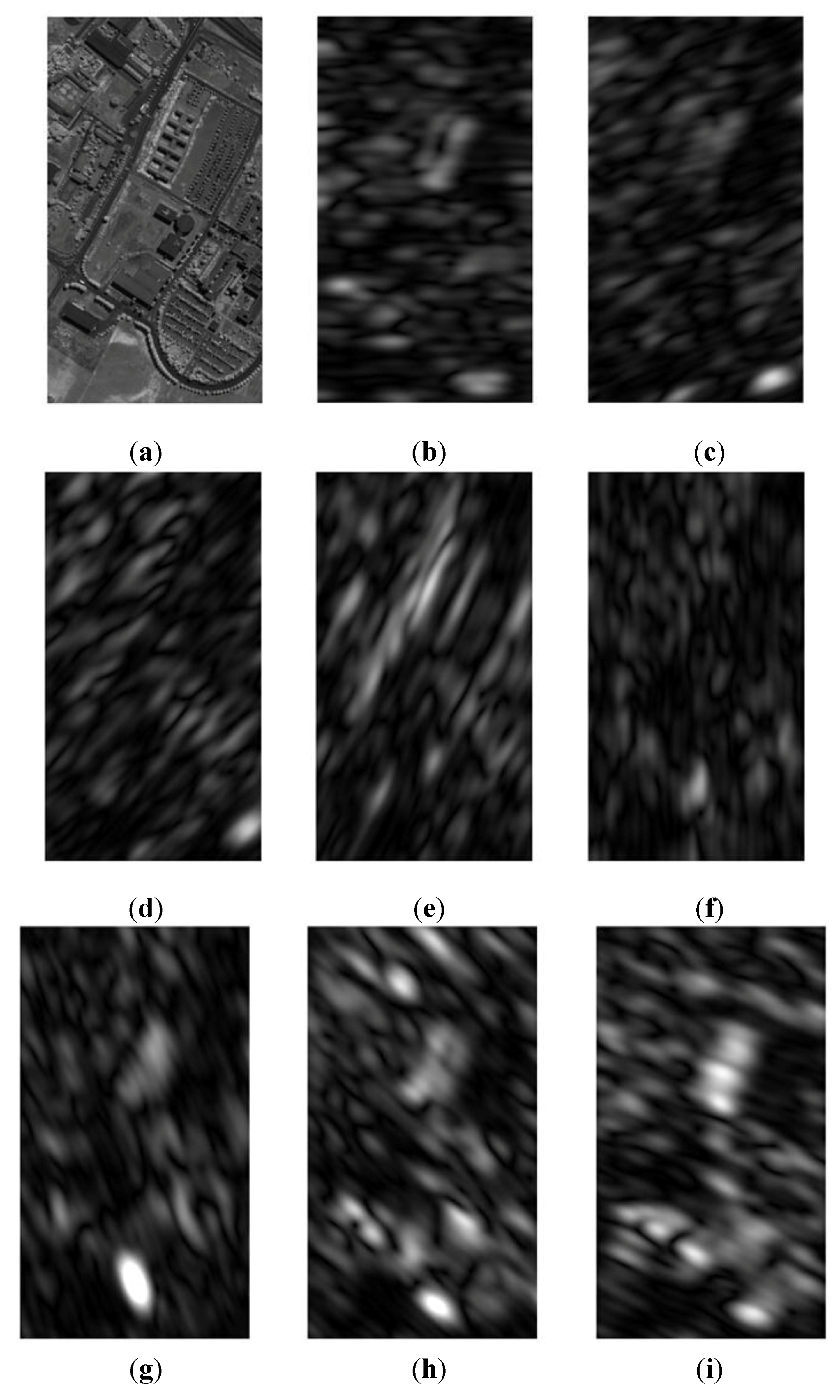
Several significant parameters for the proposed classification framework are tuned with the leave-one-out cross validation (LOOCV) strategy based on available training samples. 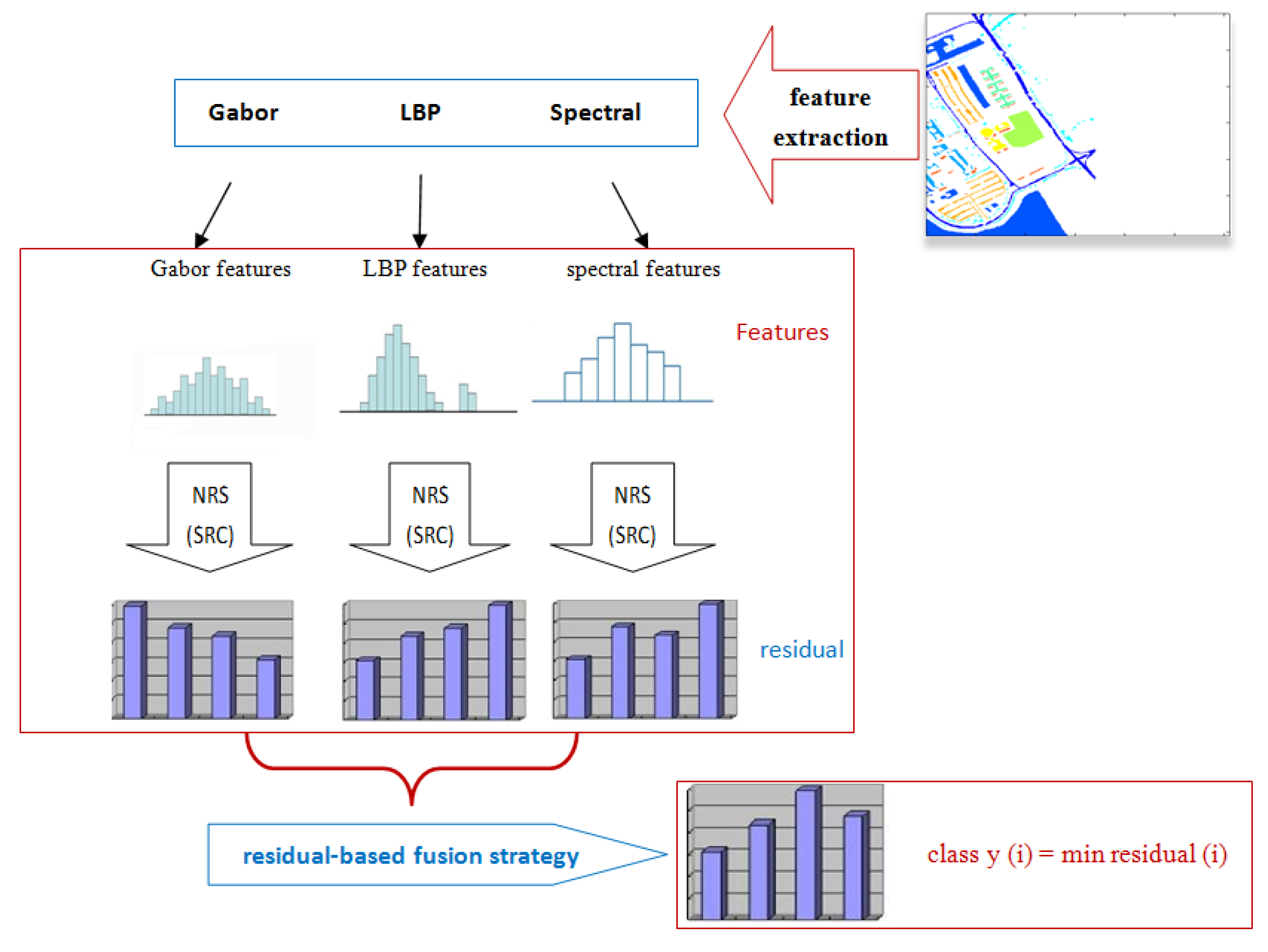For the parameters of Gabor filtering, all the eight orientations $[0，\frac{\pi }{8}，\frac{\pi }{4}，\frac{3\pi }{8}，\frac{\pi }{2}，\frac{5\pi }{8}，\frac{3\pi }{4}，\frac{7\pi }{8}]$ shown in Figure 3 are used in this work according to [47], and the parameter bw in Equation (4) is set to five and 10 bands for the Gabor filter according to our empirical study shown in Figure 4. Note that selecting more bands may not significantly improve classification accuracy, but definitely increases computational cost due to the resulting higher feature dimensionality. Thus, only three bands are selected for the LBP operator and 10 bands for the Gabor filter. 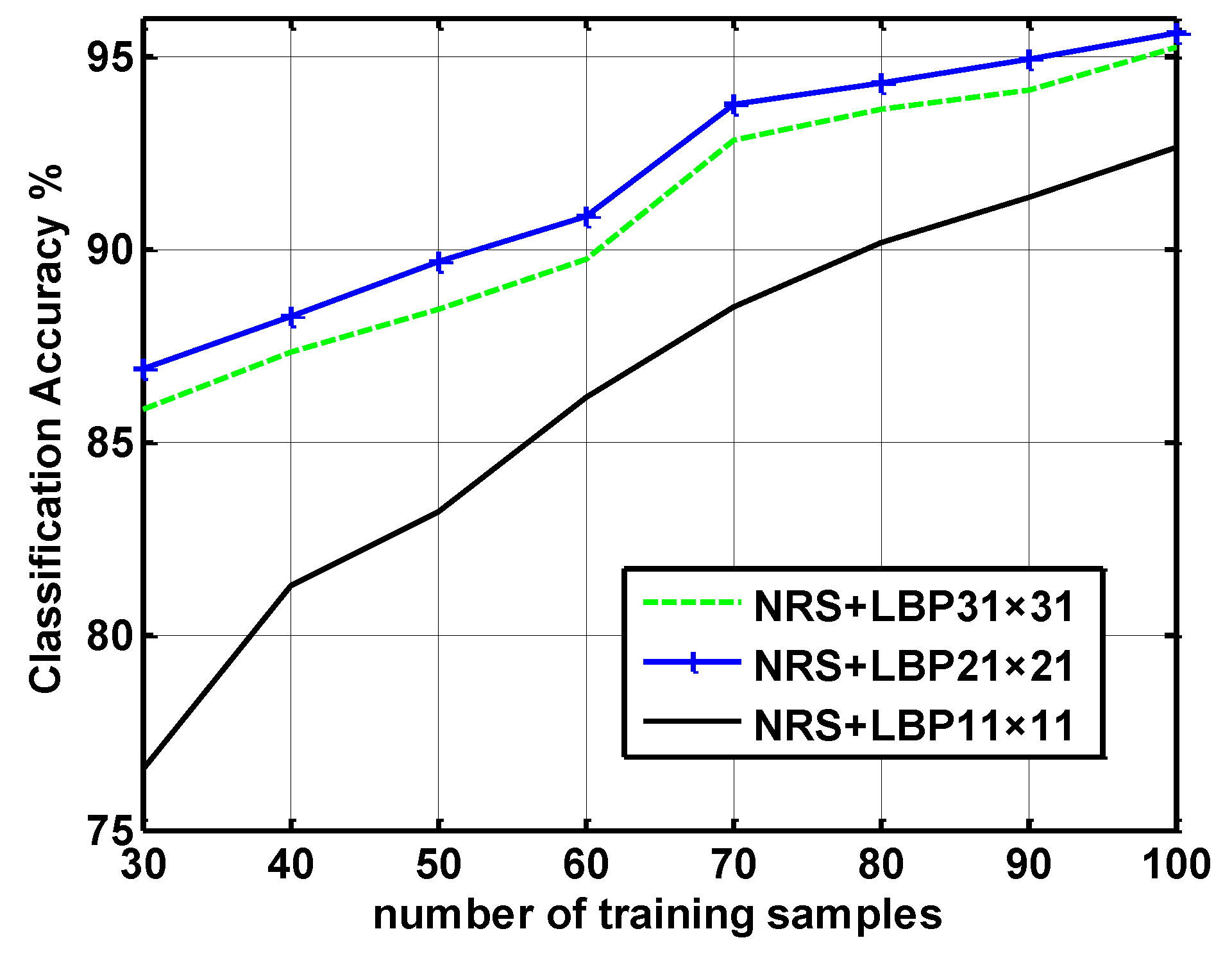Figure 5 further illustrates the effect of patch sizes on the LBP. It can be seen that classification accuracy tends to be the maximum with 21 × 21 patch size for the University of Pavia data.

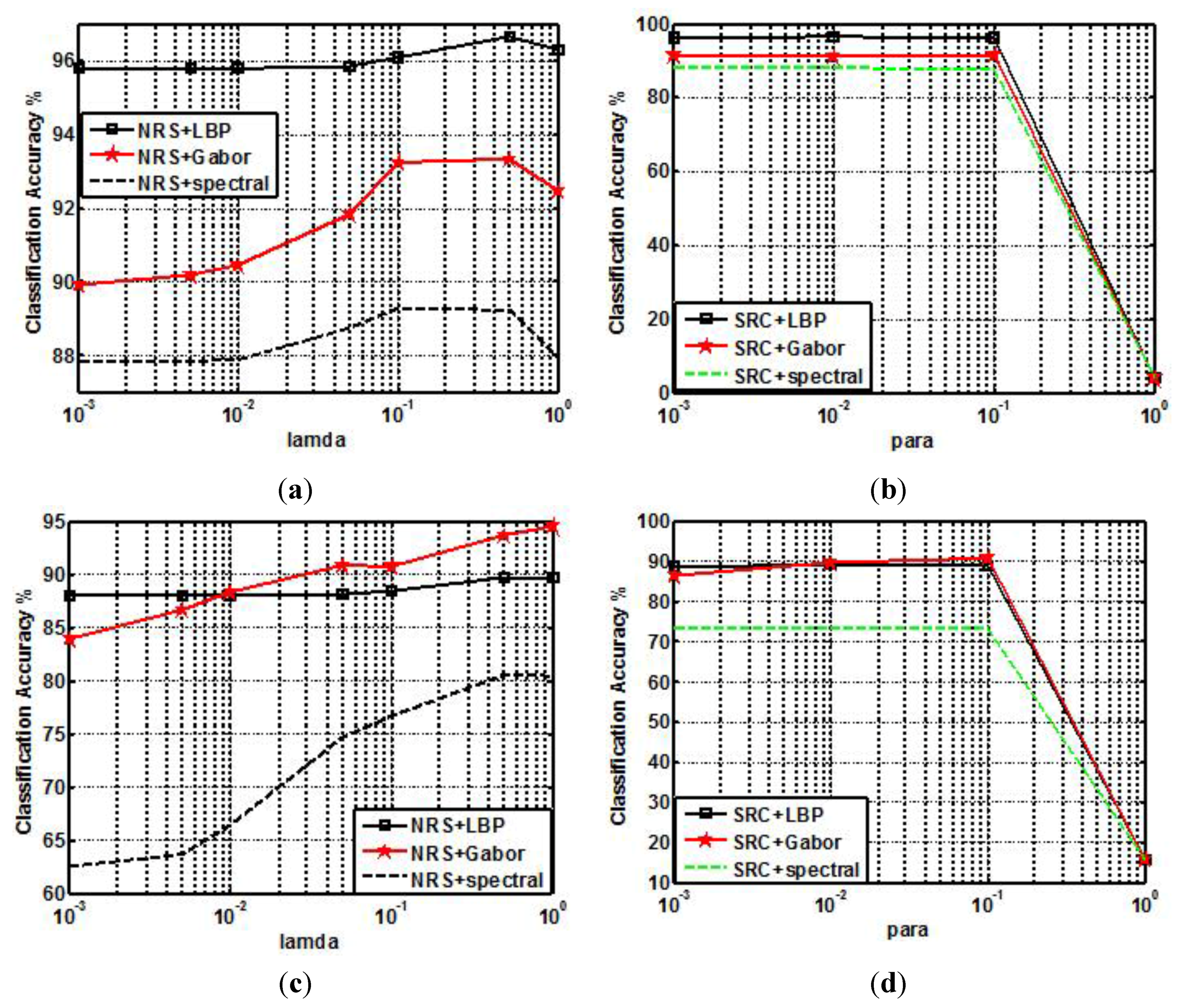
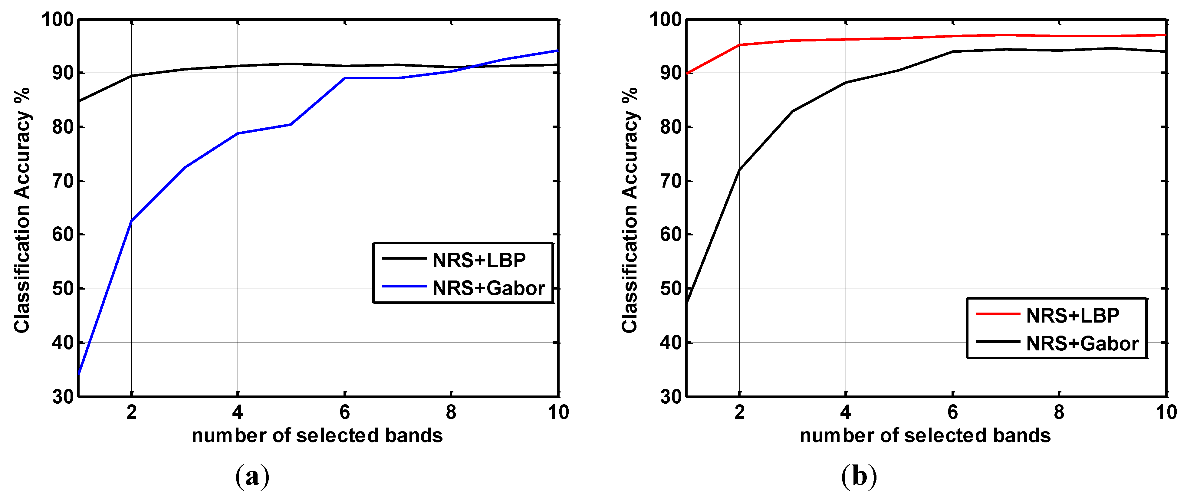
To estimate an optimal λ, Figure 6 shows accuracy at different values of λ for NRS and SRC classifiers. The number of training samples per class is 30 in the Salinas dataset, and 60 in the University of Pavia data. In different datasets, the optimal values of λ are different as shown in Figure 6. In the Salinas data, the optimal parameter is 0.5 for NRS and 0.1 for SRC; in the University of Pavia data, it is 1 for NRS and 0.1 for SRC.

Figure 3. (a) Band 95 of the University dataset. (b)–(i) Eight Gabor feature images corresponding to eight orientations of the band.

Figure 3. (a) Band 95 of the University dataset. (b)–(i) Eight Gabor feature images corresponding to eight orientations of the band.

Another three important parameters are w₁, w₂ and w₃. Table 3, Table 4, Table 5 and Table 6 demonstrate classification accuracy versus the values of w₁ and w₂. It is interesting to observe that in University of Pavia dataset, the Gabor features provide a better performance, and the LBP features need higher weights in Salinas dataset explaining the high classification accuracy of LBP-NRS in Figure 6a,b. As shown in Table 3, Table 4, Table 5 and Table 6, the best values of w₁, w₂ and w₃ are: 0.2, 0.3, 0.5; 0.6, 0.1, 0.4; 0.2, 0.7, 0.1; 0.6(0.7), 0.1, 0.3 (0.2), respectively. The weight of each residual indicates the importance of the corresponding feature. For example, in Table 3, as Gabor features perform well in the University of Pavia dataset, its weight is 0.5, much higher than the other two; in Table 4 for the Salinas dataset, where the spectral signatures actually provide the highest classification accuracy, the corresponding weight is 0.6, larger than others.

Figure 4. Classification accuracy versus the number of selected bands for: (a) University of Pavia dataset (60 training samples per class); (b) Salinas dataset (30 training samples per class).

Figure 4. Classification accuracy versus the number of selected bands for: (a) University of Pavia dataset (60 training samples per class); (b) Salinas dataset (30 training samples per class).

Figure 5. Impact of patch size on LBP generation using the University of Pavia dataset.

Figure 5. Impact of patch size on LBP generation using the University of Pavia dataset.

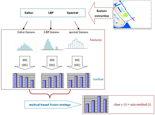
3.2. Classification Performance

The effectiveness of the proposed RF-NRS classifier is evaluated by the comparison with the original NRS [3], Gabor-NRS [16], and LBP-NRS; similarly, RF-SRC is compared with the original SRC [6], Gabor-SRC, and LBP-SRC. In the University of Pavia dataset, the number of training samples per class is varied from 30–100. In the dataset of Salinas Valley, the number of training samples per class is from 10–30. All the samples are selected randomly to avoid bias.

Figure 6. Classification accuracy (%) on two datasets using different parameters for λ: (a) and (b) Salinas dataset with 30 training samples per class, and (c) and (d) University of Pavia dataset with 60 training samples per class.

Figure 6. Classification accuracy (%) on two datasets using different parameters for λ: (a) and (b) Salinas dataset with 30 training samples per class, and (c) and (d) University of Pavia dataset with 60 training samples per class.

Table 3. Classification accuracy (%) versus the values of w₁ and w₂ for RF-NRS in University of Pavia dataset with 60 training samples per class.

	w1	0	0.1	0.2	0.3	0.4	0.5	0.6	0.7	0.8	0.9	1
w2
0		0.8257	0.9637	0.9796	0.9833	0.9835	0.9823	0.9795	0.9755	0.9667	0.9464	0.9067
0.1		0.9312	0.9813	0.9874	0.9884	0.9878	0.9855	0.9816	0.9761	0.9595	0.9248	-
0.2		0.9596	0.9872	0.9915	0.9912	0.9899	0.9874	0.9831	0.9724	0.9394	-	-
0.3		0.9697	0.989	0.9923	0.9922	0.9908	0.9873	0.981	0.9536	-	-	-
0.4		0.973	0.9888	0.9919	0.9921	0.9904	0.9856	0.9666	-	-	-	-
0.5		0.9725	0.9869	0.9908	0.9911	0.9881	0.9753	-	-	-	-	-
0.6		0.9701	0.9839	0.9878	0.9877	0.9794	-	-	-	-	-	-
0.7		0.9667	0.9797	0.9829	0.9784	-	-	-	-	-	-	-
0.8		0.9625	0.9736	0.973	-	-	-	-	-	-	-	-
0.9		0.9552	0.9626	-	-	-	-	-	-	-	-	-
1		0.9428	-	-	-	-	-	-	-	-	-	-

Table 3. Classification accuracy (%) versus the values of w₁ and w₂ for RF-NRS in University of Pavia dataset with 60 training samples per class.

	w1	0	0.1	0.2	0.3	0.4	0.5	0.6	0.7	0.8	0.9	1
w2
0		0.8257	0.9637	0.9796	0.9833	0.9835	0.9823	0.9795	0.9755	0.9667	0.9464	0.9067
0.1		0.9312	0.9813	0.9874	0.9884	0.9878	0.9855	0.9816	0.9761	0.9595	0.9248	-
0.2		0.9596	0.9872	0.9915	0.9912	0.9899	0.9874	0.9831	0.9724	0.9394	-	-
0.3		0.9697	0.989	0.9923	0.9922	0.9908	0.9873	0.981	0.9536	-	-	-
0.4		0.973	0.9888	0.9919	0.9921	0.9904	0.9856	0.9666	-	-	-	-
0.5		0.9725	0.9869	0.9908	0.9911	0.9881	0.9753	-	-	-	-	-
0.6		0.9701	0.9839	0.9878	0.9877	0.9794	-	-	-	-	-	-
0.7		0.9667	0.9797	0.9829	0.9784	-	-	-	-	-	-	-
0.8		0.9625	0.9736	0.973	-	-	-	-	-	-	-	-
0.9		0.9552	0.9626	-	-	-	-	-	-	-	-	-
1		0.9428	-	-	-	-	-	-	-	-	-	-

Table 4. Classification accuracy (%) versus the values of w₁ and w₂ for RF-NRS in Salinas dataset with 30 training samples per class.

	w1	0	0.1	0.2	0.3	0.4	0.5	0.6	0.7	0.8	0.9	1
w2
0		0.8759	0.9652	0.9795	0.9839	0.9852	0.9853	0.9856	0.9852	0.9837	0.9787	0.9667
0.1		0.9006	0.969	0.9808	0.9848	0.9856	0.9858	0.9859	0.9849	0.9817	0.9755	-
0.2		0.9174	0.969	0.9795	0.9832	0.9846	0.9855	0.9848	0.9827	0.9785	-	-
0.3		0.9301	0.969	0.9775	0.9812	0.9831	0.9836	0.982	0.9792	-	-	-
0.4		0.9374	0.9685	0.9759	0.9794	0.981	0.9811	0.9792	-	-	-	-
0.5		0.9407	0.967	0.9739	0.9773	0.9785	0.9779	-	-	-	-	-
0.6		0.941	0.9652	0.9718	0.9749	0.9756	-	-	-	-	-	-
0.7		0.9401	0.9633	0.9699	0.9716	-	-	-	-	-	-	-
0.8		0.9382	0.9609	0.967	-	-	-	-	-	-	-	-
0.9		0.9365	0.9575	-	-	-	-	-	-	-	-	-
1		0.9332	-	-	-	-	-	-	-	-	-	-

Table 4. Classification accuracy (%) versus the values of w₁ and w₂ for RF-NRS in Salinas dataset with 30 training samples per class.

	w1	0	0.1	0.2	0.3	0.4	0.5	0.6	0.7	0.8	0.9	1
w2
0		0.8759	0.9652	0.9795	0.9839	0.9852	0.9853	0.9856	0.9852	0.9837	0.9787	0.9667
0.1		0.9006	0.969	0.9808	0.9848	0.9856	0.9858	0.9859	0.9849	0.9817	0.9755	-
0.2		0.9174	0.969	0.9795	0.9832	0.9846	0.9855	0.9848	0.9827	0.9785	-	-
0.3		0.9301	0.969	0.9775	0.9812	0.9831	0.9836	0.982	0.9792	-	-	-
0.4		0.9374	0.9685	0.9759	0.9794	0.981	0.9811	0.9792	-	-	-	-
0.5		0.9407	0.967	0.9739	0.9773	0.9785	0.9779	-	-	-	-	-
0.6		0.941	0.9652	0.9718	0.9749	0.9756	-	-	-	-	-	-
0.7		0.9401	0.9633	0.9699	0.9716	-	-	-	-	-	-	-
0.8		0.9382	0.9609	0.967	-	-	-	-	-	-	-	-
0.9		0.9365	0.9575	-	-	-	-	-	-	-	-	-
1		0.9332	-	-	-	-	-	-	-	-	-	-

Table 5. Classification accuracy (%) versus the values of w₁ and w₂ for RF-SRC in University of Pavia dataset with 60 training samples per class.

	w1	0	0.1	0.2	0.3	0.4	0.5	0.6	0.7	0.8	0.9	1
w2
0		0.7359	0.8297	0.8895	0.9269	0.9495	0.962	0.9676	0.9628	0.9491	0.9278	0.901
0.1		0.7581	0.8486	0.9072	0.941	0.9607	0.9702	0.971	0.9605	0.94	0.9146	-
0.2		0.7773	0.8678	0.923	0.9537	0.9694	0.9757	0.9708	0.9537	0.9246	-	-
0.3		0.7951	0.8868	0.9383	0.9645	0.9765	0.9771	0.965	0.9387	-	-	-
0.4		0.8117	0.9045	0.9523	0.974	0.9803	0.9722	0.9531	-	-	-	-
0.5		0.8286	0.9238	0.965	0.9811	0.9771	0.9612	-	-	-	-	-
0.6		0.8457	0.942	0.9753	0.981	0.9667	-	-	-	-	-	-
0.7		0.864	0.9587	0.9814	0.9712	-	-	-	-	-	-	-
0.8		0.8854	0.9701	0.9745	-	-	-	-	-	-	-	-
0.9		0.9068	0.9678	-	-	-	-	-	-	-	-	-
1		0.9215	-	-	-	-	-	-	-	-	-	-

Table 5. Classification accuracy (%) versus the values of w₁ and w₂ for RF-SRC in University of Pavia dataset with 60 training samples per class.

	w1	0	0.1	0.2	0.3	0.4	0.5	0.6	0.7	0.8	0.9	1
w2
0		0.7359	0.8297	0.8895	0.9269	0.9495	0.962	0.9676	0.9628	0.9491	0.9278	0.901
0.1		0.7581	0.8486	0.9072	0.941	0.9607	0.9702	0.971	0.9605	0.94	0.9146	-
0.2		0.7773	0.8678	0.923	0.9537	0.9694	0.9757	0.9708	0.9537	0.9246	-	-
0.3		0.7951	0.8868	0.9383	0.9645	0.9765	0.9771	0.965	0.9387	-	-	-
0.4		0.8117	0.9045	0.9523	0.974	0.9803	0.9722	0.9531	-	-	-	-
0.5		0.8286	0.9238	0.965	0.9811	0.9771	0.9612	-	-	-	-	-
0.6		0.8457	0.942	0.9753	0.981	0.9667	-	-	-	-	-	-
0.7		0.864	0.9587	0.9814	0.9712	-	-	-	-	-	-	-
0.8		0.8854	0.9701	0.9745	-	-	-	-	-	-	-	-
0.9		0.9068	0.9678	-	-	-	-	-	-	-	-	-
1		0.9215	-	-	-	-	-	-	-	-	-	-

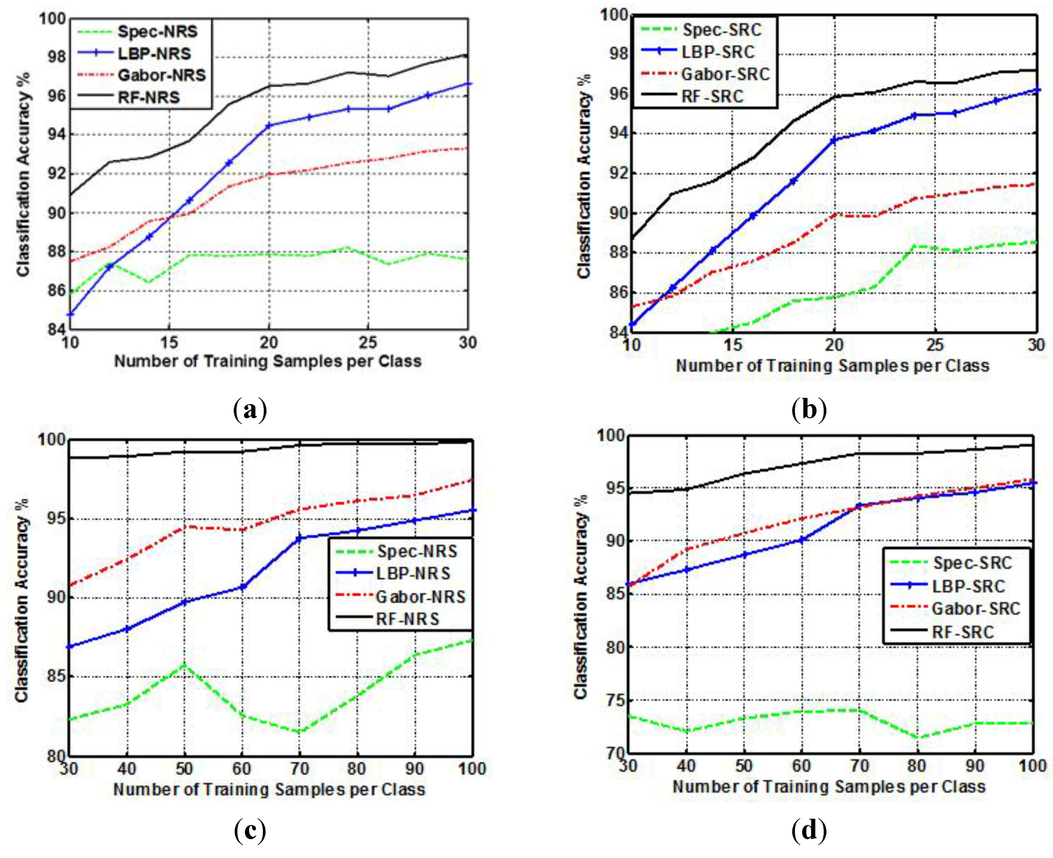
To validate the effectiveness of the proposed RF-NRS and RF-SRC, the original NRS, SRC, LBP-NRS, LBP-SRC, Gabor-NRS, and Gabor-SRC are compared. Figure 7 illustrates the classification accuracy (%) of these methods versus the number of training samples per class for the two experimental datasets. It is obvious that the accuracy of all the classifiers increases with more training samples, and the classifiers using both spectral and spatial information are much better than the one with solely spectral information. For instance, in Figure 7d, the classification accuracy of the original SRC is at least 23% lower than that of RF-SRC with 60 training samples per class. Furthermore, the proposed RF-based classifiers are consistently much better than that of LBP-NRS, Gabor-NRS, LBP-SRC, and Gabor-SRC. Taking the Salinas Valley as an example, the accuracy difference between RF-NRS and LBP-NRS is approximately 2%. When the number of training samples per class is 30 for the University of Pavia dataset, the accuracy of RF-NRS is 6% higher than the others, indicating the proposed method is more robust in SSS situations. For the Salinas dataset, Figure 7 shows that the classification accuracy of RF-SRC is 1% higher than that of LBP-SRC. For the University of Pavia dataset, RF-SRC obviously outperforms others, with an approximate 4% improvement.

Table 6. Classification accuracy (%) versus the values of w₁ and w₂ for RF-SRC in the Salinas dataset with 30 training samples per class.

	w1	0	0.1	0.2	0.3	0.4	0.5	0.6	0.7	0.8	0.9	1
w2
0		0.8853	0.9387	0.958	0.9671	0.9724	0.9753	0.9766	0.977	0.9766	0.9737	0.9622
0.1		0.888	0.9417	0.9603	0.9691	0.9736	0.9761	0.9771	0.9771	0.9756	0.9702	-
0.2		0.8901	0.9444	0.9619	0.9698	0.974	0.976	0.9763	0.9753	0.9717	-	-
0.3		0.8928	0.947	0.9635	0.9708	0.9743	0.9751	0.975	0.9717	-	-	-
0.4		0.8956	0.9502	0.9649	0.9709	0.9734	0.9741	0.9716	-	-	-	-
0.5		0.8987	0.9539	0.9665	0.9717	0.9726	0.9711	-	-	-	-	-
0.6		0.902	0.9575	0.9679	0.9709	0.97	-	-	-	-	-	-
0.7		0.9066	0.9605	0.9685	0.969	-	-	-	-	-	-	-
0.8		0.911	0.9622	0.9664	-	-	-	-	-	-	-	-
0.9		0.9161	0.9597	-	-	-	-	-	-	-	-	-
1		0.9144	-	-	-	-	-	-	-	-	-	-

Table 6. Classification accuracy (%) versus the values of w₁ and w₂ for RF-SRC in the Salinas dataset with 30 training samples per class.

	w1	0	0.1	0.2	0.3	0.4	0.5	0.6	0.7	0.8	0.9	1
w2
0		0.8853	0.9387	0.958	0.9671	0.9724	0.9753	0.9766	0.977	0.9766	0.9737	0.9622
0.1		0.888	0.9417	0.9603	0.9691	0.9736	0.9761	0.9771	0.9771	0.9756	0.9702	-
0.2		0.8901	0.9444	0.9619	0.9698	0.974	0.976	0.9763	0.9753	0.9717	-	-
0.3		0.8928	0.947	0.9635	0.9708	0.9743	0.9751	0.975	0.9717	-	-	-
0.4		0.8956	0.9502	0.9649	0.9709	0.9734	0.9741	0.9716	-	-	-	-
0.5		0.8987	0.9539	0.9665	0.9717	0.9726	0.9711	-	-	-	-	-
0.6		0.902	0.9575	0.9679	0.9709	0.97	-	-	-	-	-	-
0.7		0.9066	0.9605	0.9685	0.969	-	-	-	-	-	-	-
0.8		0.911	0.9622	0.9664	-	-	-	-	-	-	-	-
0.9		0.9161	0.9597	-	-	-	-	-	-	-	-	-
1		0.9144	-	-	-	-	-	-	-	-	-	-

Figure 7. Classification accuracy (%) versus different numbers of training samples per class for two experimental datasets: (a) and (b) Salinas Valley dataset; (c) and (d) University of Pavia dataset.

Figure 7. Classification accuracy (%) versus different numbers of training samples per class for two experimental datasets: (a) and (b) Salinas Valley dataset; (c) and (d) University of Pavia dataset.

The classification accuracy for each class and overall accuracy (OA) are listed in Table 7 and Table 8 for the two datasets. For the Salinas dataset, 30 samples are randomly selected from each class for training and the rest for testing, while for the University of Pavia dataset, the number of training samples is 60 per class. As can be seen in Table 7 and Table 8, using spatial features enhances classification accuracy. For example, in Table 7, accuracy is increased by approximately 8% with the integration of the LBP feature, and Table 8 shows the Gabor feature brings about 9% improvement. 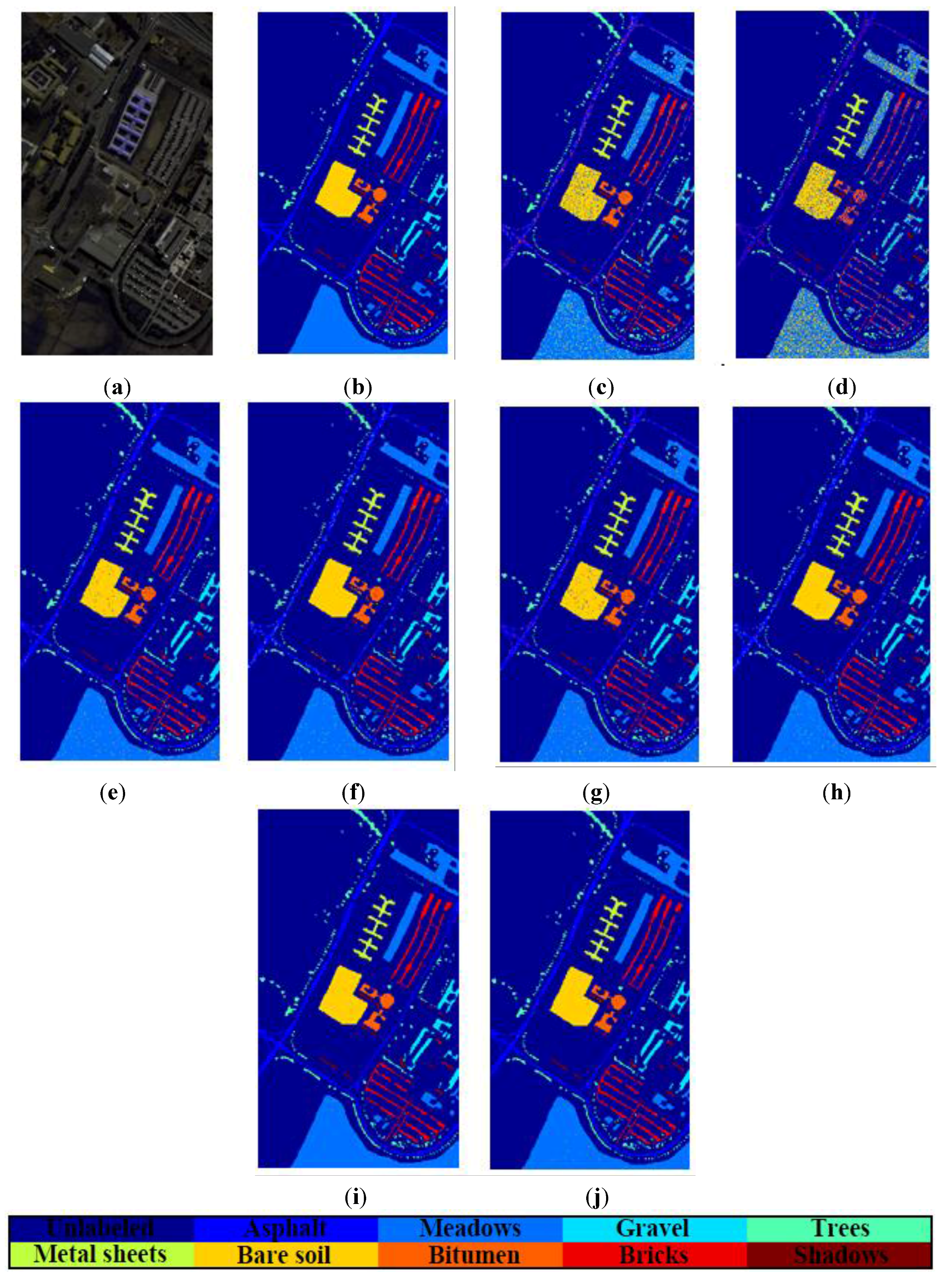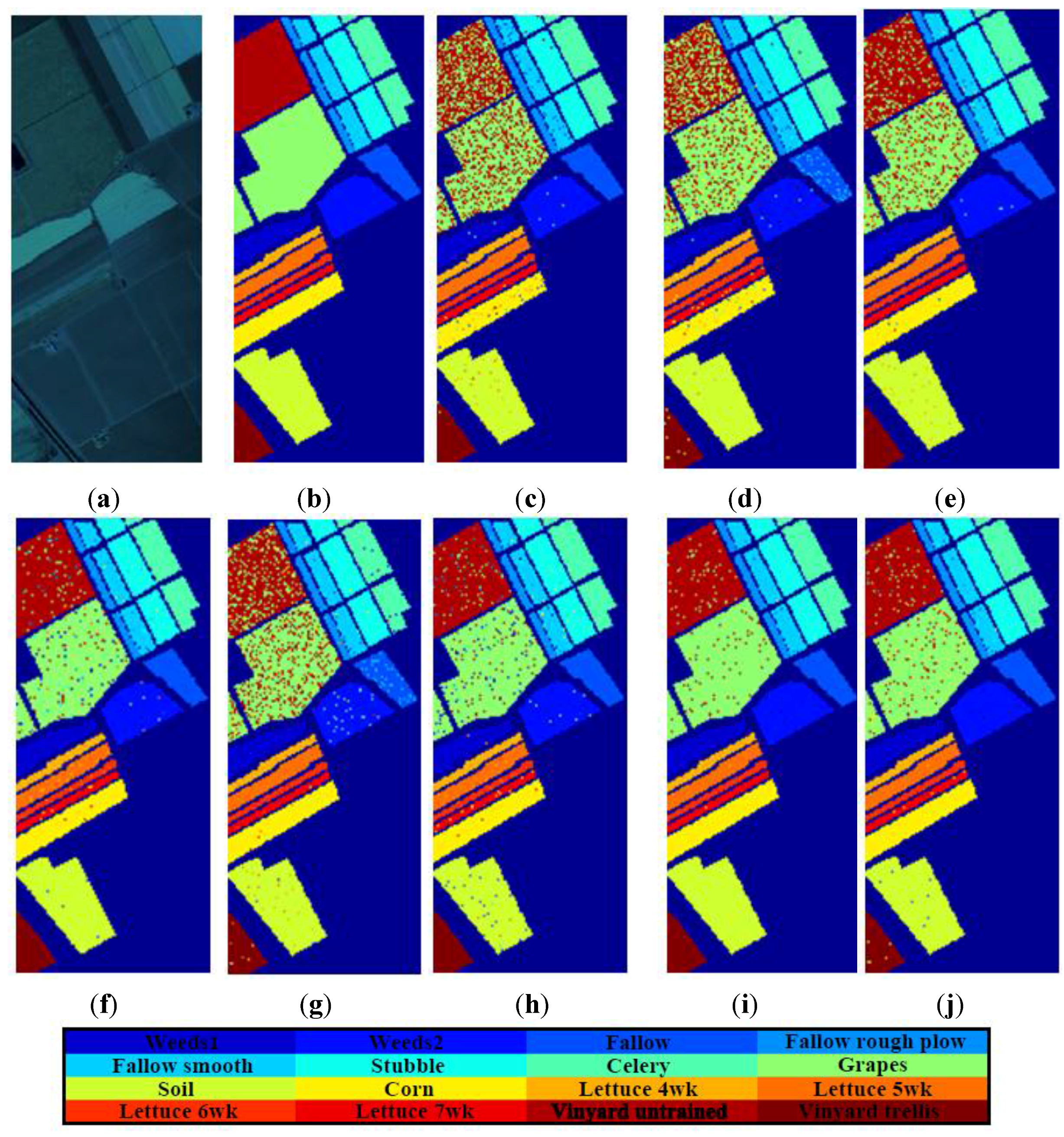Figure 8 and Figure 9 are the thematic maps of these hyperspectral datasets. Clearly, the classification maps of the proposed residual-fusion methods are less noisy and more accurate, which are consistent with the results listed in Table 7 and Table 8.

Table 7. Classification accuracy (%) for the Salinas dataset.

Class	Samples		LBP-NRS	Gabor-NRS	NRS	RF-NRS	LBP-SRC	Gabor-SRC	SRC	RF-SRC	LBP-SVM	Gabor-SVM
	Train	Test
1	30	1979	100	98.95	99.15	100	99.8	99.05	99.35	100	100	99.24
2	30	3696	97.05	96.78	99.6	99.46	96.51	94.66	92.38	99.49	94.53	96.19
3	30	1946	100	99.85	98.89	100	100	92.76	90.08	100	99.69	99.49
4	30	1364	99.28	98.13	98.49	100	98.28	98.06	99.71	99.71	95.53	97.73
5	30	2648	95.29	97.76	97.35	98.17	96.12	98.32	96.83	97.61	95.96	99.06
6	30	3929	97.17	99.97	99.42	100	97.17	99.77	99.77	99.95	97.23	99.72
7	30	3549	97.15	99.86	99.44	100	96.45	99.19	99.5	99.97	97.21	99.86
8	30	11241	93.43	78.12	69.96	94.37	92.5	79.5	79.9	91.53	93.34	77.36
9	30	6173	99.21	98.05	96.94	99.61	98.31	97.45	99.58	99.71	98.64	98.67
10	30	3248	99.39	98.23	94.87	99.97	99.33	96.77	91.76	99.66	99.38	97.14
11	30	1038	100	98.22	96.63	99.72	99.81	97.94	99.25	99.63	100	98.17
12	30	1897	96.42	100	100	100	95.9	100	98.13	99.95	97	100
13	30	886	92.9	97.16	99.67	99.34	94.21	95.74	97.16	97.6	99.23	98.87
14	30	1040	97.48	98.88	92.06	99.91	95.33	98.04	93.18	98.6	96.83	96.83
15	30	7238	94.85	84.3	73.39	96.31	94.7	79.55	60.61	94.7	92.05	84.84
16	30	1777	100	99.67	98.17	100	99.72	98.78	98.28	99.17	99.72	99.04
OA	-	-	96.67	92.45	88.87	98.14	96.22	91.44	88.53	97.2	96.01	92.29

Table 7. Classification accuracy (%) for the Salinas dataset.

Class	Samples		LBP-NRS	Gabor-NRS	NRS	RF-NRS	LBP-SRC	Gabor-SRC	SRC	RF-SRC	LBP-SVM	Gabor-SVM
	Train	Test
1	30	1979	100	98.95	99.15	100	99.8	99.05	99.35	100	100	99.24
2	30	3696	97.05	96.78	99.6	99.46	96.51	94.66	92.38	99.49	94.53	96.19
3	30	1946	100	99.85	98.89	100	100	92.76	90.08	100	99.69	99.49
4	30	1364	99.28	98.13	98.49	100	98.28	98.06	99.71	99.71	95.53	97.73
5	30	2648	95.29	97.76	97.35	98.17	96.12	98.32	96.83	97.61	95.96	99.06
6	30	3929	97.17	99.97	99.42	100	97.17	99.77	99.77	99.95	97.23	99.72
7	30	3549	97.15	99.86	99.44	100	96.45	99.19	99.5	99.97	97.21	99.86
8	30	11241	93.43	78.12	69.96	94.37	92.5	79.5	79.9	91.53	93.34	77.36
9	30	6173	99.21	98.05	96.94	99.61	98.31	97.45	99.58	99.71	98.64	98.67
10	30	3248	99.39	98.23	94.87	99.97	99.33	96.77	91.76	99.66	99.38	97.14
11	30	1038	100	98.22	96.63	99.72	99.81	97.94	99.25	99.63	100	98.17
12	30	1897	96.42	100	100	100	95.9	100	98.13	99.95	97	100
13	30	886	92.9	97.16	99.67	99.34	94.21	95.74	97.16	97.6	99.23	98.87
14	30	1040	97.48	98.88	92.06	99.91	95.33	98.04	93.18	98.6	96.83	96.83
15	30	7238	94.85	84.3	73.39	96.31	94.7	79.55	60.61	94.7	92.05	84.84
16	30	1777	100	99.67	98.17	100	99.72	98.78	98.28	99.17	99.72	99.04
OA	-	-	96.67	92.45	88.87	98.14	96.22	91.44	88.53	97.2	96.01	92.29

Table 8. Classification accuracy (%) for the University of Pavia dataset.

Class	Samples		LBP-NRS	Gabor-NRS	NRS	RF-NRS	LBP-SRC	Gabor-SRC	SRC	RF-SRC	LBP-SVM	Gabor-SVM
	Train	Test
1	60	6571	83.19	91.31	80.77	99.53	83.12	86.08	76.34	98.91	79.97	80.5
2	60	18589	92.43	94.01	84.74	98.66	91.59	93.05	66.68	94.98	89.92	90.55
3	60	2039	94.33	96.9	86.71	99.71	95.09	94.24	74.18	99.29	90.73	90.34
4	60	3004	73.89	96.87	98.4	99.45	72.32	96.61	94.39	99.35	81.95	94.49
5	60	1285	95.32	100	99.93	100	94.28	100	99.55	99.93	94.05	100
6	60	4969	97.97	96.9	82.04	99.56	96.82	94.59	83.18	99.54	98.49	95.32
7	60	1270	97.89	94.89	93.68	99.92	98.35	94.14	72.93	98.65	97.89	94.45
8	60	3622	94.62	91.09	76.75	99.76	95.06	86.23	60.97	98.32	93.06	87.78
9	60	887	83.42	95.67	99.68	99.47	83.53	94.19	100	98.1	79.82	95.09
OA	-	-	90.67	94.28	85.28	99.2	90.1	92.15	73.95	97.28	89.28	90.08

Table 8. Classification accuracy (%) for the University of Pavia dataset.

Class	Samples		LBP-NRS	Gabor-NRS	NRS	RF-NRS	LBP-SRC	Gabor-SRC	SRC	RF-SRC	LBP-SVM	Gabor-SVM
	Train	Test
1	60	6571	83.19	91.31	80.77	99.53	83.12	86.08	76.34	98.91	79.97	80.5
2	60	18589	92.43	94.01	84.74	98.66	91.59	93.05	66.68	94.98	89.92	90.55
3	60	2039	94.33	96.9	86.71	99.71	95.09	94.24	74.18	99.29	90.73	90.34
4	60	3004	73.89	96.87	98.4	99.45	72.32	96.61	94.39	99.35	81.95	94.49
5	60	1285	95.32	100	99.93	100	94.28	100	99.55	99.93	94.05	100
6	60	4969	97.97	96.9	82.04	99.56	96.82	94.59	83.18	99.54	98.49	95.32
7	60	1270	97.89	94.89	93.68	99.92	98.35	94.14	72.93	98.65	97.89	94.45
8	60	3622	94.62	91.09	76.75	99.76	95.06	86.23	60.97	98.32	93.06	87.78
9	60	887	83.42	95.67	99.68	99.47	83.53	94.19	100	98.1	79.82	95.09
OA	-	-	90.67	94.28	85.28	99.2	90.1	92.15	73.95	97.28	89.28	90.08

Figure 8. Thematic maps for the University of Pavia dataset with 60 training samples per class; (a) Pseudo-color Image; (b) Ground truth Map; (c) NRS; (d) SRC; (e) NRS + Gabor; (f) NRS + LBP; (g) SRC + Gabor; (h) SRC + LBP; (i) RF-NRS; (j) RF-SRC.

Figure 8. Thematic maps for the University of Pavia dataset with 60 training samples per class; (a) Pseudo-color Image; (b) Ground truth Map; (c) NRS; (d) SRC; (e) NRS + Gabor; (f) NRS + LBP; (g) SRC + Gabor; (h) SRC + LBP; (i) RF-NRS; (j) RF-SRC.

Figure 9. Thematic maps for the Salinas dataset with 30 training samples per class; (a) Pseudo-color Image; (b) Ground truth Map; (c) NRS; (d) SRC; (e) NRS + Gabor; (f) NRS + LBP; (g) SRC + Gabor (h) SRC + LBP; (i) RF-NRS; (j) RF-SRC.

Figure 9. Thematic maps for the Salinas dataset with 30 training samples per class; (a) Pseudo-color Image; (b) Ground truth Map; (c) NRS; (d) SRC; (e) NRS + Gabor; (f) NRS + LBP; (g) SRC + Gabor (h) SRC + LBP; (i) RF-NRS; (j) RF-SRC.

Classification results from the aforementioned classifiers using the Indian Pines data are shown in Table 9 with the same number of training and testing samples as in [48]. It is apparent that the proposed RF-NRS and RF-SRC still provide superior performance, which further affirms that classification accuracy can be greatly improved by fusing two complementary spatial features (i.e., Gabor features and LBP features).

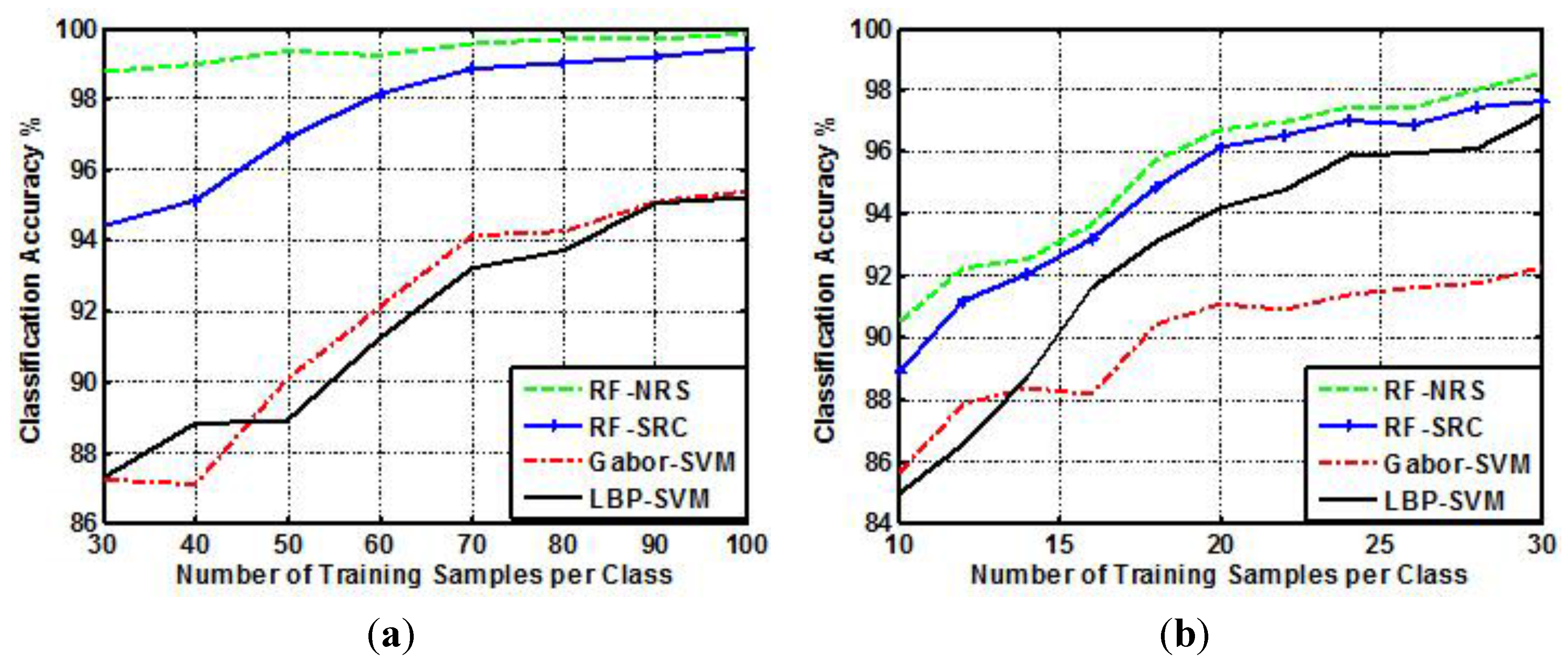
In Figure 10, the classification results of the proposed methods are compared with SVM using spatial features, i.e., LBP-SVM [49] and Gabor-SVM [50]. As can be seen, the classification accuracy of RF-NRS is more than 1% higher than that of RF-SRC. It is due to the calculation of weight coefficients is sparse in SRC, which is prone to misclassify a testing sample when the number of training samples is limited or the quality of training samples is poor. The proposed RF-NRS and RF-SRC have higher classification accuracy (at least 4%) than Gabor-SVM and LBP-SVM especially in the University of Pavia dataset. Moreover, with the increase of the number of training samples, the proposed RF-NRS and RF-SRC outperform Gabor-SVM and LBP-SVM. It also illustrates that the residual-based fusion methods provide even more solid and robust performance in SSS situations (e.g., 30 training samples per class).

Table 9. Classification accuracy (%) for the Indian Pine dataset.

Class	Samples		LBP-NRS	Gabor-NRS	RF-NRS	LBP-SRC	Gabor-SRC	RF-SRC	SVM-LBP	SVM-Gabor
	Train	Test
1	15	39	100	96.3	90.74	100	96.3	100	100	94.87
2	50	1384	87.95	80.06	92.68	88.21	71.69	91	86.63	77.96
3	50	784	97.72	90.65	98.56	96.88	81.77	98.44	98.47	88.61
4	50	184	100	98.72	99.15	98.72	95.3	99.15	99.46	100
5	50	447	97.18	96.58	98.99	97.18	93.96	97.79	97.99	94.85
6	50	697	97.59	96.92	97.99	96.92	93.04	98.8	96.7	97.56
7	15	11	100	100	100	100	100	100	100	100
8	50	439	100	100	100	100	100	100	100	100
9	15	5	100	100	100	100	100	100	100	100
10	50	918	86.88	85.12	90.39	88.02	82.54	88.33	86.93	75.49
11	50	2418	89.67	82.46	94.04	89.26	78.08	88.53	86.35	73.9
12	50	574	91.21	93.16	97.72	91.53	94.3	95.93	90.6	90.43
13	50	162	99.06	98.11	100	98.58	98.58	99.53	100	99.38
14	50	1244	96.99	93.66	99	97.76	95.29	99.69	97.51	96.78
15	50	330	99.21	96.32	100	99.47	95.53	100	99.39	98.18
16	50	45	100	100	100	100	100	100	100	100
OA	-	-	93.16	89.12	96.04	93.23	85.73	94.31	92.08	85.43

Table 9. Classification accuracy (%) for the Indian Pine dataset.

Class	Samples		LBP-NRS	Gabor-NRS	RF-NRS	LBP-SRC	Gabor-SRC	RF-SRC	SVM-LBP	SVM-Gabor
	Train	Test
1	15	39	100	96.3	90.74	100	96.3	100	100	94.87
2	50	1384	87.95	80.06	92.68	88.21	71.69	91	86.63	77.96
3	50	784	97.72	90.65	98.56	96.88	81.77	98.44	98.47	88.61
4	50	184	100	98.72	99.15	98.72	95.3	99.15	99.46	100
5	50	447	97.18	96.58	98.99	97.18	93.96	97.79	97.99	94.85
6	50	697	97.59	96.92	97.99	96.92	93.04	98.8	96.7	97.56
7	15	11	100	100	100	100	100	100	100	100
8	50	439	100	100	100	100	100	100	100	100
9	15	5	100	100	100	100	100	100	100	100
10	50	918	86.88	85.12	90.39	88.02	82.54	88.33	86.93	75.49
11	50	2418	89.67	82.46	94.04	89.26	78.08	88.53	86.35	73.9
12	50	574	91.21	93.16	97.72	91.53	94.3	95.93	90.6	90.43
13	50	162	99.06	98.11	100	98.58	98.58	99.53	100	99.38
14	50	1244	96.99	93.66	99	97.76	95.29	99.69	97.51	96.78
15	50	330	99.21	96.32	100	99.47	95.53	100	99.39	98.18
16	50	45	100	100	100	100	100	100	100	100
OA	-	-	93.16	89.12	96.04	93.23	85.73	94.31	92.08	85.43

Figure 10. Classification accuracy (%) versus the number of training samples per class for: (a) University of Pavia dataset; (b) Salinas dataset.

Figure 10. Classification accuracy (%) versus the number of training samples per class for: (a) University of Pavia dataset; (b) Salinas dataset.

4. Conclusions

In this paper, a weighted-residual-fusion-based classification framework was proposed. The overall classification utilized multiple features, including LBP features, Gabor features, and the original spectral features. A representation-based classifier, such as NRS or SRC, was applied to each type of feature, and fusion was achieved by a weighted combination of their residuals. It was found that the resulting classifiers, i.e., RF-NRS and RF-SRC, were more discriminative than the original spectral classifiers and the classifiers with the Gabor feature and the LBP feature only. Experimental results from several real hyperspectral images demonstrated that the proposed residual-fusion-based classification methods consistently outperformed the traditional classifiers and other state-of-the-art classification algorithms (e.g., Gabor-SVM and LBP-SVM) when the number of training samples per class was varied. Specifically, the proposed RF-NRS achieved about 6% classification accuracy improvement over the traditional Gabor-NRS and Gabor-SVM, and about 2% over the LBP-NRS and LBP-SVM for the Salinas dataset when 30 training samples per class were chosen. RF-NRS outperformed Gabor-NRS by about 5%, LBP-NRS by about 9%, LBP-SVM by about 10%, and Gabor-SVM by about 9% for the University of Pavia data when 60 training samples per class were chosen. In addition, the proposed RF-NRS and RF-SRC tended to be more robust in SSS situations.

In future work, the spectral-local-global feature fusion strategy will be exploited with more state-of-the-art features, and automatic estimation of optimal/suboptimal weighting parameters will be investigated.

References

1. Landgrebe, D.A. Hyperspectral image data analysis. IEEE Signal Process. Mag. 2002, 19, 17–28. [Google Scholar] [CrossRef]
2. Li, W.; Prasad, S.; Fowler, J.E. Decision fusion in kernel-induced spaces for hyperspectral image classification. IEEE Trans. Geosci. Remote Sens. 2014, 52, 3399–3411. [Google Scholar] [CrossRef]
3. Li, W.; Tramel, E.W.; Prasad, S.; Fowler, J.E. Nearest regularized subspace for hyperspectral classification. IEEE Trans. Geosci. Remote Sens. 2014, 52, 477–489. [Google Scholar] [CrossRef]
4. Wright, J.; Ma, Y.; Mairal, J.; Sapiro, G.; Huang, T.S.; Yan, S. Sparse representation for computer vision and pattern recognition. Proc. IEEE. 2010, 98, 1031–1044. [Google Scholar] [CrossRef]
5. Wright, J.; Yang, A.; Ganesh, A.; Sastry, S.; Ma, Y. Robust face recognition via sparse representation. IEEE Trans. Pattern Anal. Mach. Intell. 2009, 31, 210–227. [Google Scholar] [CrossRef] [PubMed]
6. Zhang, H.; Nasrabadi, N.; Zhang, Y.; Huang, T. Joint Dynamic Sparse Representation for Multiview Face Recognition. Pattern Recognit. 2012, 45, 1290–1298. [Google Scholar] [CrossRef]
7. Chen, Y.; Nasrabadi, M.; Tran, T. Hyperspectral image classification using dictionary-based sparse representation. IEEE Trans. Geosci. Remote Sens. 2011, 49, 3973–3985. [Google Scholar] [CrossRef]
8. Tang, Y.; Li, X.; Liu, Y.; Wang, J.; Liu, C.; Liu, S. Hyperspectral image classification using sparse representation-based classifier. In Proceedings of the IEEE International Geoscience and Remote Sensing Symposium (IGARSS), Quebec City, QC, Canada, 13–18 July 2014; pp. 3450–3453.
9. Iordache, M.; Bioucas-Dias, J.; Plaza, A. Sparse unmixing of hyperspectral data. IEEE Geosci. Remote Sens. 2011, 49, 2014–2039. [Google Scholar] [CrossRef]
10. Sun, X.; Qu, Q.; Nasrabadi, N.M.; Tran, T.D. Structured priors for sparse-representation-based hyperspectral image classification. IEEE Geosci. Remote Sens. Lett. 2014, 11, 1235–1239. [Google Scholar] [CrossRef]
11. Berg, E.; Friedlander, M. Joint-sparse recovery from multiple measurements. IEEE Trans. Inf. Theor. 2010, 56, 2516–2527. [Google Scholar] [CrossRef]
12. Liu, G.; Lin, Z.; Yan, S.; Sun, J.; Yu, Y.; Ma, Y. Robust recovery of subspace structures by low-rank representation. IEEE Trans. Pattern Anal. Mach. Intell. 2013, 35, 171–184. [Google Scholar] [CrossRef] [PubMed]
13. Sprechmann, P.; Ramirez, I.; Sapiro, G.; Eldar, Y. C-HiLasso: A collaborative hierarchical sparse modeling framework. IEEE Trans. Signal Process. 2011, 59, 4183–4198. [Google Scholar] [CrossRef]
14. Camps-Valls, G.; Gomez-Chova, L.; Muñoz-Marí, J.; Vila-Francés, J.; Calpe-Maravilla, J. Composite kernels for hyperspectral image classification. IEEE Geosci. Remote Sens. Lett. 2006, 3, 93–97. [Google Scholar] [CrossRef]
15. Song, B.; Li, J.; Dalla Mura, M.; Li, P.; Plaza, A.; Bioucas-Dias, J.M.; Benediktsson, J.A.; Chanussot, J. Remotely sensed image classification using sparse representations of morphological attribute profiles. IEEE Trans. Geosci. Remote Sens. 2014, 52, 5122–5136. [Google Scholar] [CrossRef]
16. Li, W.; Du, Q. Gabor-filtering-based nearest regularized subspace for hyperspectral image classification. IEEE J. Sel. Top. Appl. Earth Observ. Remote Sens. 2014, 7, 1012–1022. [Google Scholar] [CrossRef]
17. Jia, S.; Jia, L.; Li, Q. Gabor feature-based collaborative representation for hyperspectral imagery classification. IEEE Trans. Geosci. Remote Sens. 2015, 52, 1118–1129. [Google Scholar]
18. Tsai, F.; Tsai, J.S. Feature extraction of hyperspectral image cubes using three dimensional gray level co-occurrence. IEEE Trans. Geosci. Remote Sens. 2013, 5, 3504–3514. [Google Scholar] [CrossRef]
19. Li, W.; Chen, C.; Su, H.; Du, Q. Local binary patterns and extreme learning machine for hyperspectral image classification. IEEE Trans. Geosci. Remote Sens. 2015, 53, 3681–3693. [Google Scholar] [CrossRef]
20. Quesada-Barriuso, P.; Arguello, F.; Heras, D.B. Spectral-Spatial Classification of Hyperspectral Images Using Wavelets and Extended Morphological Profiles. Sel. Top. Appl. Earth Observ. Remote Sens. 2014, 7, 1177–1185. [Google Scholar] [CrossRef]
21. Ghamisi, P.; Benediktsson, J.A.; Gavallaro, G.; Plaza, A. Automatic Framework for Spectral-Spatial Classification Based on Supervised Feature Extraction and Morphological Attribute Profiles. Sel. Top. Appl. Earth Observ. Remote Sens. 2014, 7, 2147–2160. [Google Scholar] [CrossRef]
22. Rajadell, O.; Garcia-Sevilla, P.; Pla, F. Spectral-Spatial Pixel Characterization Using Gabor Filters for Hyperspectral Image Classification. IEEE Geosci. Remote Sens. Lett. 2013, 10, 860–864. [Google Scholar] [CrossRef]
23. Zhang, L.; Zhang, L.; Tao, D.; Huang, X. On combining multiple features for hyperspectral remote sensing image classification. IEEE Trans. Geosci. Remote Sens. 2012, 50, 879–893. [Google Scholar] [CrossRef]
24. Xiong, M.; Ran, Q.; Li, W.; Zou, J.; Du, Q. Hyperspectral image classification using weighted joint collaborative representation. IEEE Geosci. Remote Sens. Lett. 2015, 12, 1209–1213. [Google Scholar] [CrossRef]
25. Lee, H.; Chung, Y.; Yoo, J.H.; Won, C. Face recognition based on sparse representation classifier with gabor-edge components histogram. In Proceedings of the 8th International Conference on Signal Image Technology and Internet Based Systems (SITIS), Naples, Italy, 25–29 November 2012; pp. 105–109.
26. Li, W.; Du, Q. Joint within-class collaborative representation for hyperspectral image classification. Sel. Top. Appl. Earth Observ. Remote Sens. 2014, 7, 2200–2208. [Google Scholar] [CrossRef]
27. Tropp, J.A.; Gilbert, A.C.; Strauss, M.J. Algorithms for simultaneous sparse approximation. Part I: Greedy pursuit. IEEE Signal Process. 2006, 86, 572–588. [Google Scholar] [CrossRef]
28. Wang, J.; Jiao, L.; Liu, H.; Yang, S.; Liu, F. Hyperspectral image classification by spatial-spectral derivative-aided kernel joint sparse representation. IEEE J. Sel. Top. Appl. Earth Observ. Remote Sens. 2015, 8, 2485–2500. [Google Scholar] [CrossRef]
29. Fang, L.; Li, S.; Kang, X.; Benediktsson, J.A. Spectral-spatial hyperspectral image classification via multiscale adaptive sparse representation. IEEE Trans. Geosci. Remote Sens. 2014, 52, 7738–7749. [Google Scholar] [CrossRef]
30. Waske, B.; Linden, S.; Benediktsson, J.A.; Rabe, A.; Hostert, P. Sensitivity of support vector machines to random feature selection in classification of hyperspectral data. IEEE Trans. Geosci. Remote Sens. 2010, 48, 2880–2889. [Google Scholar] [CrossRef]
31. Su, H.; Sheng, Y.; Du, P.; Liu, K. Adaptive affinity propagation with spectral angle mapper for semi-supervised hyperspectral band selection. Appl. Opt. 2012, 51, 2656–2663. [Google Scholar] [CrossRef] [PubMed]
32. Alajlan, N.; Bazi, Y.; Melgani, F.; Yager, R.R. Fusion of supervised and unsupervised learning for improved classification of hyperspectral images. Inf. Sci. 2012, 217, 39–55. [Google Scholar] [CrossRef]
33. Yang, H.; Du, Q.; Ma, B. Decision fusion on supervised and unsupervised classifiers for hyperspectral imagery. IEEE Geosci. Remote Sens. Lett. 2010, 7, 875–879. [Google Scholar] [CrossRef]
34. Li, W.; Du, Q. Decision fusion for dual-window based hyperspectral anomaly detection. J. Appl. Remote Sens. 2015, 9. [Google Scholar] [CrossRef]
35. Li, W.; Liu, K.; Su, H. Wavelet-based nearest-regularized subspace for noise-robust hyperspectral image classification. J. Appl. Remote Sens. 2014, 8, 083665. [Google Scholar] [CrossRef]
36. Su, H.; Yong, B.; Du, P.; Liu, H.; Chen, C.; Liu, K. Dynamic classifier selection using spectral-spatial information for hyperspectral image classification. J. Appl. Remote Sens. 2014, 8, 085095. [Google Scholar] [CrossRef]
37. Chi, Y.; Porikli, F. Classification and boosting with multiple collaborative representations. IEEE Trans. Pattern Anal. Mach. Intell. 2014, 36, 1519–1531. [Google Scholar] [CrossRef] [PubMed]
38. Daugman, J.G. Uncertainty relation for resolution in space, spatial frequency, and orientation optimized by two-dimensional visual cortical filters. J. Optim. Soc. Am. 1985, 2, 1160–1169. [Google Scholar] [CrossRef]
39. Ojala, T.; Pietikainen, M.; Maenpaa, T.T. Multi resolution gray scale and rotation invariant texture classification with local binary pattern. IEEE Trans. Pattern Anal. Mach. Intell. 2002, 24, 971–987. [Google Scholar] [CrossRef]
40. Ahonen, T.; Hadid, A.; Pietikainen, M. Face description with local binary patterns: Application to face recognition. IEEE Trans. Pattern Anal. Mach. Intell. 2006, 28, 2037–2041. [Google Scholar] [CrossRef] [PubMed]
41. Ren, J.; Jiang, X.; Yuan, J. Noise-resistant local binary pattern with an embedded error-correction mechanism. IEEE Trans. Image Process. 2013, 22, 4049–4060. [Google Scholar] [CrossRef] [PubMed]
42. The l1_ls Package. Available online: https://stanford.edu/~boyd/l1_ls/ (accessed on 17 June 2015).
43. Du, Q.; Yang, H. Similarity-based unsupervised band selection for hyperspectral image analysis. IEEE Geosci. Remote Sens. Lett. 2008, 5, 564–568. [Google Scholar] [CrossRef]
44. Yang, H.; Du, Q.; Chen, G. Unsupervised hyperspectral band selection using graphics processing units. IEEE J. Sel. Top. Appl. Earth Observ. Remote Sens. 2011, 4, 660–668. [Google Scholar] [CrossRef]
45. Hyprespectral Remote Sensing Scenes. Available online: http://www.ehu.eus/ccwintco/index.php?title=Hyprespectral_Remote_Sensing_Scenes (accessed on 17 June 2015).
46. Gamba, P. A collection of data for urban area characterization. In Proceedings of the IEEE International Geoscience and Remote Sens. Symposium, Anchorage, AK, USA, 20–24 September 2004; pp. 69–72.
47. Chen, C.; Li, W.; Su, H.; Liu, K. Spectral-spatial classification of hyperspectral image based on kernel extreme learning machine. Remote Sens. 2014, 6, 5795–5814. [Google Scholar] [CrossRef]
48. Fauvel, M.; Tarabalka, Y.; Benediktsson, J.A.; Chanussot, J.; Tilton, J.C. Advances in spectral-spatial classification of hyperspectral images. Proc. IEEE 2013, 101, 652–675. [Google Scholar] [CrossRef]
49. Tian, Q.; Tian, G. Development and testing of a LBP-SVM based teeth visibility recognizer. In Proceedings of the IEEE International Conference on Computational Intelligence for Measurement Systems and Applications (CIMSA), Tianjin, China, 2–4 July 2012; pp. 114–119.
50. Huang, D.; Hu, W.; Chang, S. Vision-based hand gesture recognition using PCA + Gabor Filters and SVM. In Proceedings of the 5th International Conference on Intelligent Information Hiding and Multimedia Signal Processing (IIH-MSP’09), Kyoto, Japan, 12–24 September 2009; pp. 1–4.