Impact of Surface Waves on SWOT’s Projected Ocean Accuracy

Abstract

The Surface Water and Ocean Topography (SWOT) mission being considered by NASA has, as one of its main objectives, to measure ocean topography with centimeter scale accuracy over kilometer scale spatial resolution. This paper investigates the impact of ocean waves on SWOT’s projected performance. Several effects will be examined: volumetric decorrelation, aliasing of ocean waves, backscattering modulation, and the so-called surfboard sampling.

1. Introduction

The main oceanographic objective of the proposed Surface Water and Ocean Topography (SWOT) mission [1,2,3,4] is to characterize the ocean mesoscale and sub-mesoscale geostrophic circulation by providing two-dimensional measurements of Sea Surface Height (SSH) for spatial wavelengths of 15 km and larger. Even when optimally configured, current nadir altimeter constellations can only resolve the two-dimensional ocean circulation at resolutions larger than 200–300 km due to gaps between the altimeter tracks (e.g., [5]), although somewhat smaller scales can be resolved in the along-track direction . Fundamental questions on the dynamics of two-dimensional ocean variability at scales shorter than 300 km, the mesoscale and submesoscale processes such as the formation, evolution, and dissipation of eddy variability (including narrow currents, fronts, and quasi-geostrophic turbulence) and its role in air-sea interaction, are to be addressed by these new observations. Global studies of the circulation in the scales between 15 and 300 km are essential for quantifying the kinetic energy of ocean circulation and the ocean uptake of climate relevant tracers such as heat and carbon [4]. The SWOT mission will the first spaceborne mission to provide direct measurements of SSH at these scales, opening a new window on these dynamics.

The primary instrument enabling the SWOT measurement is the Ka-band Radar Interferometer (KaRIn) [3,4] which is complemented with a nadir-looking altimeter and a three-frequency microwave radiometer, as well as a GPS receiver and a DORIS transponder for precise orbit determination. Several error sources limit the accuracy of the measurement, most notably thermal noise, waves, baseline roll drift, and wet tropospheric path delay errors. These can be loosely split into those creating random errors, which are destructive in nature and cannot be corrected on the ground, and systematic errors, which could be theoretically removed if all fields (waves, media, spacecraft attitude, etc.) were perfectly known. This paper focuses on the impact of surface waves on SWOT’s projected ocean accuracy.

Since radar range resolution is basically timing resolution [6], two spatially separated points that arrived at the same time at the radar receiver cannot not be resolved and the two points are said to be “laid-over” [6]. The problem of surface layover in interferometry is well known [7,8], and leads to an increase in the random noise due to decorrelation and to biases in the estimated height. To first order, if the radar footprint is large compared to the spatial scale of height variability, the effect of ocean waves on scattering can be viewed as being due to an effective volume scattering layer. Under this approximation, Rodríguez and Martin [7] were able to derive a formula for the height biases (including the well-known electromagnetic or EM bias), as well as for the increase in random height noise due to volumetric decorrelation. The contribution of the present paper consists of examining the case when the ocean surface wavelength is not smaller than the radar range footprint, but on the same order or larger. We show that when sampling in the near-range direction, additional non-linear effects appear which have not been discussed previously in the literature. When the angle of incidence is smaller than the wave slope (i.e., for incidence angles of a few degrees, depending on sea state [9]) the iso-range plane will cut the wave field at multiple points, like a long surfboard in choppy seas. We call this non-linear sampling effect surfboard sampling, which is not only relevant to SWOT but also applies to other near-nadir systems, such as AirSWOT (an airborne calibration/validation platform for SWOT).

In this paper, we argue that the surfboard sampling introduces two distorting effects. The first one is due to the relation that exists between sampling using planes tilted relative to the horizontal reference versus uniform spatial sampling, which occurs along planes orthogonal to the horizontal. The tilted plane sampling will intersect the surface at irregular spatial intervals, but evenly spaced range. For high-resolution interferometers, this effect is usually accounted for by using the high-resolution phase to geolocate the unevenly sampled points and regrid them via interpolation. Unfortunately, to reduce data downlink, SWOT uses an Onboard Processor (OBP) to average the interferogram to 250 m–1 km sampling, and in this averaging step information is lost that would allow the high-resolution resampling step. In effect, SWOT assumes that the ocean’s surface is flat enough so that points that are evenly sampled in range are also evenly sampled in space. This approximation introduces spectral distortion errors, discussed below. The second effect occurs when the tilted planes intersect the surface at multiple points which have different heights, giving rise to “layover” [6]. To first order, this layover effect reduces interferometric correlation and increases height noise, as described in [7]. However, unlike volume scattering from homogeneous layers, the spatial aliasing introduced by this many-to-one mapping results in distortions of the measured SSH spectrum, which can introduce artificial spectral “bumps” even at the low frequencies where the SSH mesoscale and submesoscale signals reside. This uneven sampling also impacts the electromagnetic bias in interferometry, since it samples certain slopes of the waves preferentially, so that it couples to the hydrodynamic and tilt modulations [10]. In this paper, the impact of backscatter modulation is also incorporated.

There have been previous studies of the measurement of elevations of surface wave fields, most notably [11,12,13,14,15,16,17]. However, these studies were done for high resolution systems sampling at moderate incidence angles. Furthermore, for SWOT we are concerned with effects that are centimetric or smaller, so the effects described in this paper would not have been important for the previous studies.

We also note that many of the studies done previously deal with the distortions due to forming synthetic apertures over times that are significant relative to the wave period (see, for instance [13]), leading to wave bunching effects in the azimuth direction [14]. For SWOT, only very short apertures are formed (250 m azimuth resolution), so that these nonlinear azimuthal effects can be neglected compared to the distortions introduced by range sampling.

The paper is organized as follows. Section 2, Section 3 and Section 4 explain the nature of the ocean wave induced errors. Section 5 includes results of extensive simulations using spectra from a wave prediction model, namely WAVEWATCH-III, which is routinely used by the National Oceanic and Atmospheric Administration (NOAA) for marine weather forecasting and the U.S. Navy for fleet operations planning [18]. Finally, Section 6 presents an assessment of the impact of waves on the projected SWOT error. An approximate first-order mathematical derivation for the surfboard sampling and backscattering modulation is included in the Appendix.

2. Volumetric Wave Decorrelation

At Ka band there is practically no penetration of the radar radiation into the water. However, the scatterers follow the surface topography, which in the case of waves presents high variability within a range resolution cell, especially in the near range. To first order, if the radar footprint is large compared to the spatial scale of height variability, the effect of ocean waves on scattering can be viewed as due to an effective volume scattering layer. In order to quantify the impact of the volume scattering introduced by the waves, and following a similar approach as presented by Rodriguez and Martin [7], we model the statistics of the ocean surface height with a Gaussian probability function, $f_s\left(h\right)=\frac{1}{\sqrt{2\pi {\sigma }_h^2}}{e}^{-\frac{h^2}{2{\sigma }_h^2}}$ where h is the topographic mean height at a given point, and ${\sigma }_h$ is the ocean height standard deviation, which is, relative, related to the significant wave height as $SWH=4{\sigma }_h$ [19]. The interferometric phase, $\Phi$, is approximately given by [7,8]:

$$\Phi \approx {\kappa }_{z}h$$

(1)

where ${\kappa }_z=\frac{k_{0}B\cos {\theta }_0}{r\sin {\theta }_i}$, ${\theta }_0$ is the look angle for a target at a given range distance, $r$, ${\theta }_i$ is the incidence angle, $B$ is the baseline length, and $k_0$ is the RF signal wavenumber.

The volumetric decorrelation between the interferometric channels, which determines the height noise increase due to surface waves [7], can then be shown to be given by:

$${\gamma }_{SWH}\cong {{\displaystyle \int }}^{\text{}}{e}^{j{\kappa }_{z}h}{f}_s\left(h\right)dh=e^{-\frac{1}{2}{\kappa }_z^2{\sigma }_h^2}$$

(2)

Figure 1 illustrates the decorrelation due to volume scattering from a Gaussian distributed layer as a function of cross track distance for different values of significant wave height (SWH) [9,10]. As a comparison, the black dashed curve shows the SWOT’s projected correlation due to noise only. From these curves it becomes apparent that this effect can have substantial impact on the random height performance in the near swath as the SWH increases. Using the probability density function for SWH, which has been derived from one year of WAVEWATCH-III spectra (shown in the insert), the expected volume scattering decorrelation averaged over global SWH conditions is computed and shown in black. This expected value roughly matches the curve for SWH = 3, which incidentally is approximately the 1-sigma (68%) value for the SWH distribution.

Figure 1. Decorrelation due to volume scattering from a Gaussian distributed layer as a function of cross track distance for different values of significant wave height (SWH). The black solid curve is the expected volume scatter correlation averaged over global SWH conditions modeled using one year of WAVEWATCH-III data (insert contains the SWH probability density function). The black dashed curve illustrates the decorrelation due to noise only for comparison. The total decorrelation is the product of these two decorrelation factors, and also the smaller geometric/angular decorrelation [20].

Figure 1. Decorrelation due to volume scattering from a Gaussian distributed layer as a function of cross track distance for different values of significant wave height (SWH). The black solid curve is the expected volume scatter correlation averaged over global SWH conditions modeled using one year of WAVEWATCH-III data (insert contains the SWH probability density function). The black dashed curve illustrates the decorrelation due to noise only for comparison. The total decorrelation is the product of these two decorrelation factors, and also the smaller geometric/angular decorrelation [20].

3. Wave Spectrum Aliasing

A conventional SAR measures the location of a target in a two-dimensional coordinate system, with one axis along the flight track (“along-track direction”) and the other axis defined as the range from the SAR to the target (“range direction”). A SAR resolves targets in the range direction by measuring the time it takes a radar pulse to propagate to the target and return to the radar. The along-track location is determined from the Doppler frequency shift that results whenever the relative velocity between the radar and target is not zero [21,22,23,24]. To obtain three-dimensional position information, an additional measurement of elevation angle is needed. Interferometry using two or more SAR images provides a means of determining this angle [7,8].

The raw echo data rate is determined by the sampling frequency; the number of bits used to digitize the analog signal, the pulse repetition frequency (PRF), and swath extent. For KaRIn, this totals about 3.5 Gbps. Since it is prohibitive to downlink this amount of data over the global ocean, a critical component of KaRIn is an on-board processor (OBP) that produces the complex interferogram and SAR amplitude images averaged down to a resolution of 1 km with 1 km posting, reducing the downlink data rate by about three orders of magnitude. This averaging step comprises filtering to the 1km resolution and decimation to a 1 km posting. Most of the wave energy is concentrated at wavelengths less than ~300 m, with the dominant wavelength dependent on wind speed. However, the frequency response of a finite length filter exhibits sidelobes beyond the cut-off frequency [25,26], and some of the wave spectrum energy at short wavelengths will be aliased to longer wavelengths during the decimation step, introducing a residual height error, the so-called wave spectrum aliasing height error. In this section we present a simplified derivation of the effect. A comprehensive analysis is included in the Appendix.

The height measured by KaRIn is approximately given by the convolution of the ocean wave height, $h\left(x,y\right)$, and KaRIn’s interferometric point target response (PTR) [7,8]. For simplicity, let us consider a one dimensional wave field (it is straightforward to generalize the result to an arbitrary wave field), so the measured height, $h_m$, can be expressed as:

$$h_m\left(x_0\right)\approx {{\displaystyle \int }}^{\text{}}dx h\left(x\right) \chi \left(x-x_0\right)$$

(3)

where $\chi \left(x\right)$ is KaRIn’s interferometric PTR along $x$. The average height over a resolution cell using a spatial weighting function $w\left(x\right)$ is obtained as follows:

$$\overline{h_m}\left(x_o\right)={{\displaystyle \int }}^{\text{}}dxw\left(x-x_0\right)h_m\left(x\right)$$

(4)

where $w\left(x\right)$ is normalized such that ${{\displaystyle \int }}^{\text{}}dxw\left(x\right)=1$.

For a one-dimensional continuous wave spectrum, the surface height can be written as:

$$h\left(x\right)=\frac{1}{2\pi }{{\displaystyle \int }}^{\text{}}dk\tilde{h}\left(k\right)e^{ik\cdot x}$$

(5)

where k is the ocean wave-number, and $\tilde{h}\left(k\right)$ is the complex wave amplitude, related to the wave spectrum, $S_h\left(k\right)$, by $\langle \tilde{h}\left(k\right){\tilde{h}}^{*}\left(k\text{'}\right)\rangle =S_h\left(k\right)\delta \left(k-k^{\prime }\right)$.

For illustrative purposes, let us assume $\chi \left(x\right)$ is a sinc-squared function of intrinsic resolution $B_x$, $\chi \left(x\right)=\frac{1}{B_x}{\text{sinc}}^2\frac{x}{B_x}$ [7]. It can be shown that the average height error due to wave spectrum aliasing is given by:

$$\langle {\overline{h_m}}^2\rangle \approx \frac{1}{2\pi }{{\displaystyle \int }}_{\raisebox{1ex}{$\pi $}\!\left/ \!\raisebox{-1ex}{$P$}\right.}^{\infty }dk S_h\left(k\right){\left|W\left(k\right)\text{Λ}\left(\frac{B_x}{2\pi }k\right)\right|}^2$$

(6)

where $\text{Λ}\left(k\right)$ is the triangular function defined as $\text{Λ}\left(k\right)=\text{max }\left(1-\left|k\right|,0\right)$, $W\left(k\right)$ is the Fourier transform of $w\left(x\right)$, and $P$ is the posting (1 km).

The window length is determined by the desired ocean pixel final resolution, where resolution is defined such that the auto-correlation at ± half the pixel resolution is 0.5. This ensures an equivalent number of independent pixels such that if further multi-looking (during ground post-processing) is performed, the resulting variance of the multi-look pixel is inversely proportional to the number of pixels used. Posting is defined as distance between consecutive pixels. Equation (6) indicates that the amount of wave energy that is aliased into the measured signal is determined by the system resolution, the radar transfer function, the averaging window, and the posting.

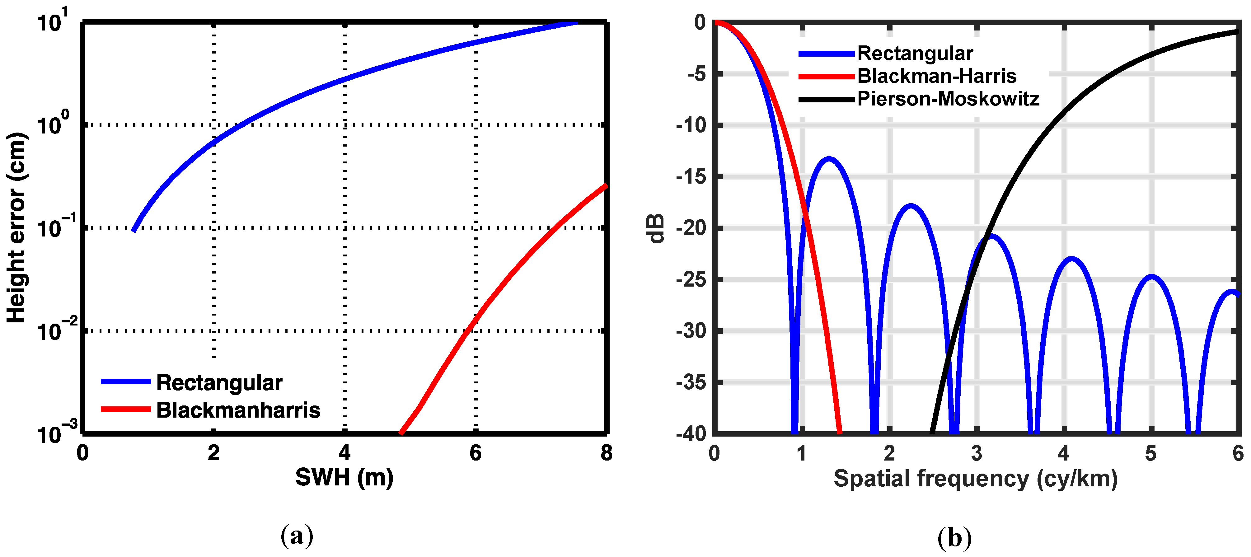
In order to assess the impact of the aliased height, a wind driven Pierson-Moskowitz wave spectrum for fully developed seas [27] is assumed in the following calculations in worst case conditions, namely that the waves are traveling along a single direction aligned with the averaging direction. Figure 2a illustrates the residual height error due to wave aliasing for two different windows, a rectangular window and a Blackman-Harris [26] window (Figure 2b), as a function of significant wave height (SWH). By using a smoothing window, the error is reduced by several orders of magnitude relative to the unweighted (rectangular) case. Note that for a rectangular window, the window length equals the pixel resolution, whereas for a Blackman-Harris window, the window length is roughly twice the pixel resolution, so computations are performed over overlapping segments.

Figure 2. (a) Residual height error due to wave spectrum aliasing for rectangular (blue) and Blackman-Harris (red) windows as a function of SWH. (b) Spectral response for rectangular (blue) and Blackman-Harris (red) windows in comparison to ocean wave energy as predicted by a Pierson-Moskowitz wind driven spectrum (in black, normalized to maximum) for SWH = 3 m.

Figure 2. (a) Residual height error due to wave spectrum aliasing for rectangular (blue) and Blackman-Harris (red) windows as a function of SWH. (b) Spectral response for rectangular (blue) and Blackman-Harris (red) windows in comparison to ocean wave energy as predicted by a Pierson-Moskowitz wind driven spectrum (in black, normalized to maximum) for SWH = 3 m.

4. Tilted Plane Sampling and Backscattering Modulation

Radars sample three-dimensional space by intersecting spheres that are the loci of points arriving at the same time at the radar receiver, and cones that are the loci of points having the same Doppler shift [21,22,23,24]. Radar interferometers add an additional dimension, the interferometric phase difference, to provide the additional degree of freedom needed to map from radar space into physical space [7,8]. While this mapping function is generally a well behaved one-to-one mapping, it can breakdown in special points, called “layover” points, when multiple points in physical space map to a single point in radar space [7,8,15].

In most situations, one images away from the nadir point, and acquires data close to zero Doppler. In these circumstances, which apply to patches of SWOT data over which the incidence angle can be regarded as approximately constant, the sampling in the range direction can be visualized as given by the intersection of the surface and a set of parallel planes, or surfboards, with a tilt equal to the angle of incidence relative to the mean surface. 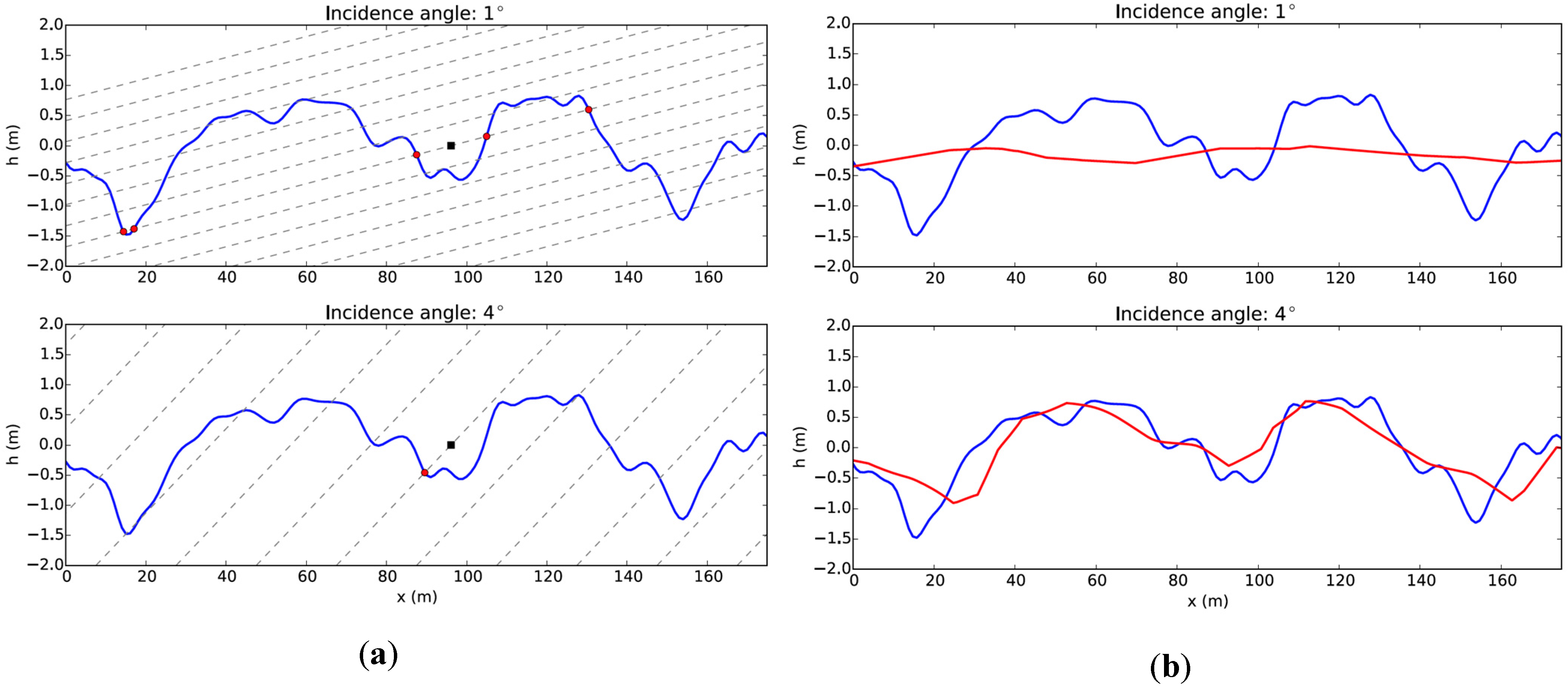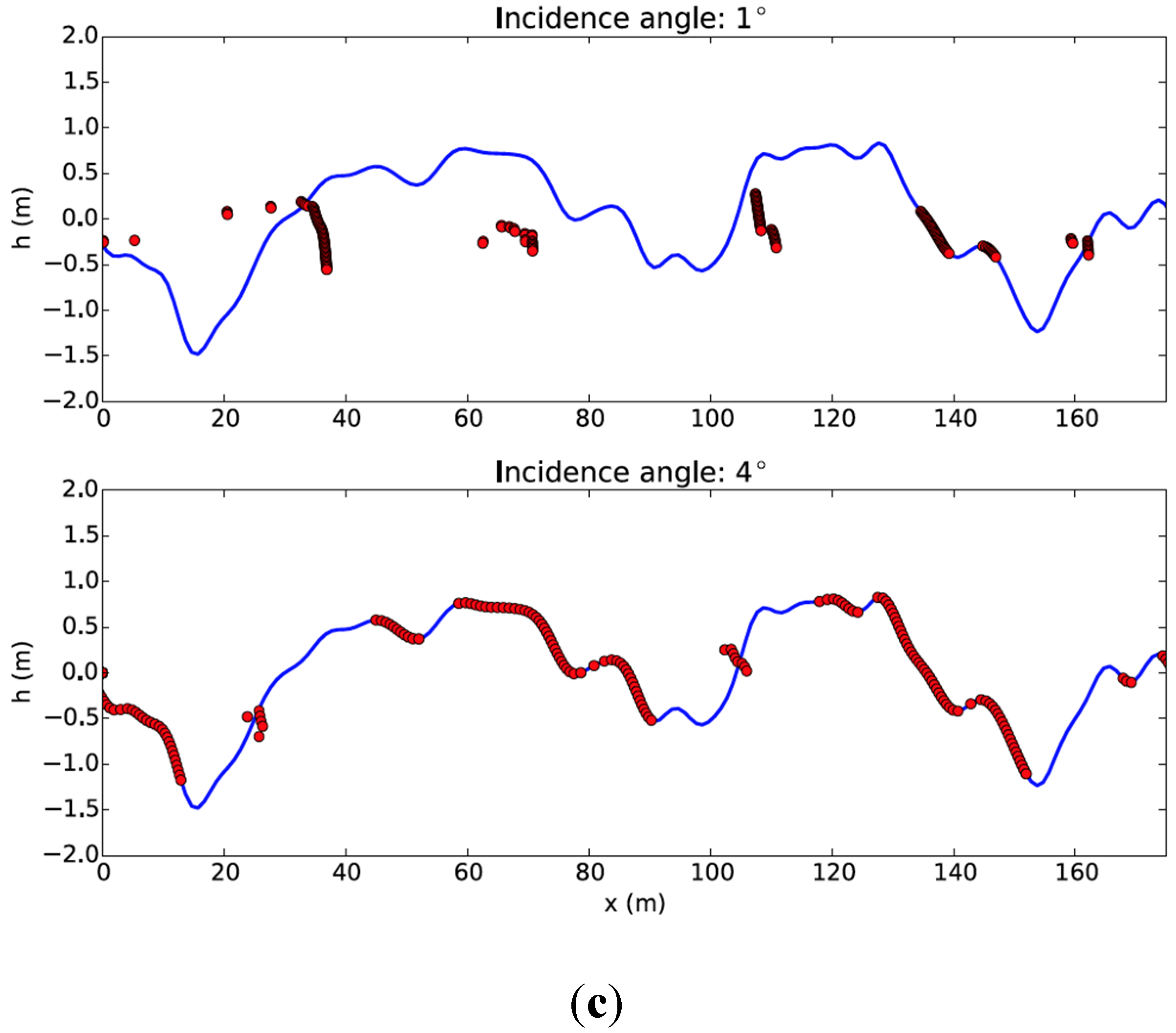This geometry is illustrated in Figure 3a for a single realization of a wave field with Pierson-Moskowitz spectrum and significant wave height of about 3 m, for two incidence angles that roughly correspond to SWOT’s near and far range. Two effects are readily apparent from this picture. First, and especially for the shallower incidence angle, the same sampling plane can cut the surface at multiple locations, giving rise to layover points (red circles, in the figure). The separation between layover points (up to 100 m in this example) depends on the radar incidence angle, SWH, and the ocean wave peak wavelength. The second effect is due to the fact that the wave slopes facing the radar are sampled with different frequency than the slopes facing away from the radar, so faces that normally point towards the radar are foreshortened, while the faces pointing away are stretched. Figure 3b exemplifies the measured height compared to the true height, where the apparent smoothing is the result of the convolution of the surface impulse response with the point target response. When layover is prevalent, the surface height is underestimated and severely distorted by the averaging of surface heights separated by large distances. However, even when no actual layover occurs, the waves are distorted because the faces pointing towards the radar have significantly smaller sample density compared to the ones pointing away from the radar. This is further demonstrated in Figure 3c, where, assuming a noiseless measurement, the measured heights were used to estimate the true cross-track coordinate. When there is significant layover, as for the small incidence angle and for the faces pointing towards the radar, the estimated cross-track coordinate, which is the average of the cross-track coordinate of the layover points, is not valid. When no layover is present, we see that using the estimated cross-track coordinate allows the faithful reconstruction of the surface, albeit with non-uniform sampling: the faces pointing towards the radar have significantly smaller sample density compared to the ones pointing away from the radar. This non-uniform sampling will also have implications on the EM bias.

Figure 3. (a) Simulated Pierson-Moskowitz ocean wave field (U10=10m/s) propagating in the range direction (blue) and sampled by a set of parallel planes (dashed gray) separated by 20 m in range. The top figure represents the sampling when the local incidence angle is 1°, while the bottom figure shows the same wave field when the incidence angle is 4°. The intersection of a sample plane with the mean level is shown as a black square, while the sampled heights are shown as red circles. The radar is on the left and the radar pulses propagate from left to right. (b) True (blue) and measured (red) heights for wave field presented in (a) for a system with finite resolution bandwidth (surface impulse response), plotted as a function of the intersection of the range coordinate with the mean surface. (c) Estimated height as a function of estimated cross track, assuming a noiseless measurement.

Figure 3. (a) Simulated Pierson-Moskowitz ocean wave field (U10=10m/s) propagating in the range direction (blue) and sampled by a set of parallel planes (dashed gray) separated by 20 m in range. The top figure represents the sampling when the local incidence angle is 1°, while the bottom figure shows the same wave field when the incidence angle is 4°. The intersection of a sample plane with the mean level is shown as a black square, while the sampled heights are shown as red circles. The radar is on the left and the radar pulses propagate from left to right. (b) True (blue) and measured (red) heights for wave field presented in (a) for a system with finite resolution bandwidth (surface impulse response), plotted as a function of the intersection of the range coordinate with the mean surface. (c) Estimated height as a function of estimated cross track, assuming a noiseless measurement.

The spectral content of the wave spectra is concentrated at wavelengths well below 2 km (i.e., twice the posting), which is filtered by a weighted average filtering stage as discussed in the previous section. However, due to the surfboard sampling, the measured height is a nonlinear function of the wave height, which introduces nonlinear spectral distortions. Powers of the wave height are equivalent to convolutions of the wave spectrum with itself. Therefore, nonlinear products of the wave height result in wave energy spreading to wavelengths greater than 2 km, which are not filtered and become a significant contribution to the height error.

Another nonlinear contribution to the height error arises from the backscattering modulation. For near-nadir scattering at Ka-band, it is appropriate, to lowest order, to use the geometrical optics backscatter cross section [28]. The effect of the large-scale waves is to provide a tilt modulation as follows:

$${\sigma }_0\cong \frac{R^2}{s^2}{e}^{-\frac{{\left({\theta }_i-h_s\right)}^2}{s^2}}$$

(7)

where $R^2$ is the Fresnel reflectivity factor, $s^2$ is the surface wave slope variance, ${\theta }_i$ is the incidence angle for the mean surface, and $h_s$ is the long wave slope. The geometrical optics cross section is thus modulated by the value of the wave slope in two ways. First, the large-scale surface wave determines the local incidence angle and results in the cross section tilt modulation [10,17]. In addition, the small-scale wave slope variance, which is the principal contributor to $s^2$, is modulated by the large-scale waves, resulting in an additional hydrodynamic modulation. In this paper, we assume a simple model for the hydrodynamic modulation [10,17], namely that the normalized backscattering, $\delta \sigma =\frac{{\sigma }_0-\overline{{\sigma }_0}}{\overline{{\sigma }_0}}$, is modulated by the normalized wave height, $\frac{h}{{\sigma }_h}$, as [10]:

$$\delta \sigma =-4\beta \frac{h}{{\sigma }_h}$$

(8)

This simplified model is a good approximation to the mean modulation of the cross section observed (or modeled) to contribute to the EM bias, although for any given wave realization there will be deviations (uncorrelated with the height) due to non-linearity of the wave interactions. Although only approximate, this model is sufficient to demonstrate the non-linear sampling phenomena we are examining. A full assessment of realistic EM bias will require better models for both tilt and hydrodynamic modulations to take into account non-linear ocean features in modulation and slope [10,19].

It follows from this model that the parameter $\beta$ [19] relates the EM bias and the SWH as:

$$EMbias=\beta \cdot SWH$$

(9)

where it is implicit that the bias is negative. Measurements at Ka band indicate the EM bias ranges from 1% to 3% of the SWH [19].

The backscattering in Equation (8) modulates the radar response such that measured height is a nonlinear function of the wave height, in a similar fashion as the surfboard sampling, also spreading the wave energy to longer wavelengths that are not filtered.

A first-order mathematical formulation for the impact of the surfboard and the backscattering modulation is included in the Appendix. We show that the surfboard height error is approximately inversely proportional to the ground range, and that there is no impact on the electromagnetic bias associated with the surfboard sampling. Our theory also predicts that the effect is stronger for waves aligned with the cross track direction, and vanishes for waves aligned in the along-track direction. The backscattering modulation height error is approximately independent of wave direction and ground range, and the EM bias follows to first order Equation (9). The height errors due to the surfboard sampling and the backscattering modulation add in an root mean square (RMS) fashion.

However, for large wave fields and in the near range, some of the first order theory assumptions are no longer valid. First, the interferometric phase cannot be assumed to be linearly proportional to height as in Equation (1), and therefore averaging the interferogram (i.e., $~e^{j\Phi }$) is not equivalent to averaging the heights. In fact, the phase might even undergo multiple 2π wraps within an averaging interval. With interferometry and sufficiently high signal to noise ratio (SNR), the true location of the targets could be obtained and this effect partially mitigated, but this is not possible for SWOT’s OBP due to the computational complexity and the level of thermal noise. In addition, layover is strong and is coupled with the brightness modulation. These second order effects result in height errors and biases that approximately increase as the inverse of ground range distance squared. A more detailed analytical investigation of these second order effects will be the subject of future investigation, but the simulations in this and the following sections illustrate the magnitude of this error.

Ocean waves have complex two-dimensional spectra with wave energy spreading both in frequency and space. However, a better understanding of the impact of the surfboard can be gained by studying the height error for a one-dimensional spectrum at different wave directions relative to the spacecraft boresight direction. In this section we assume a Pierson-Moskowitz spectrum. The radar response has been characterized using an interferometric simulator that also includes the response of the on-board processor.

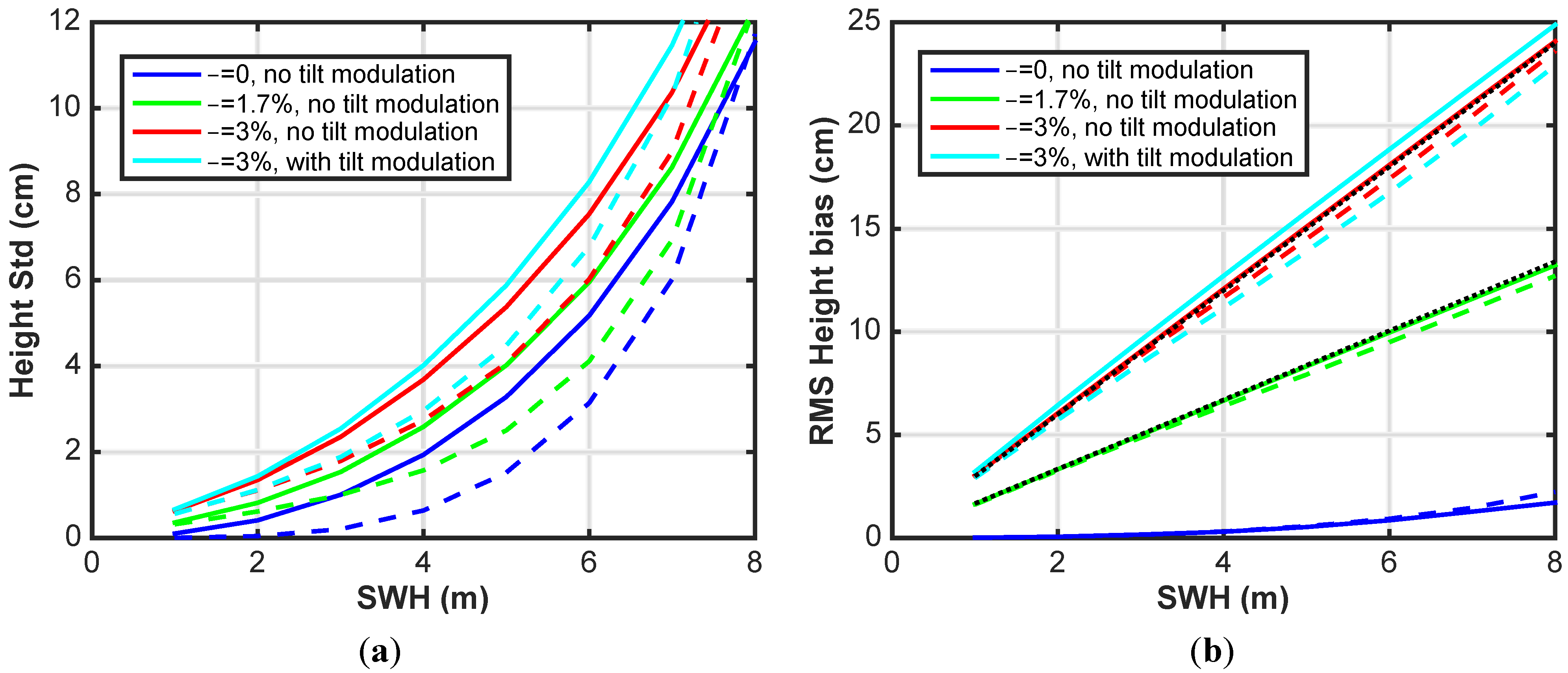
Figure 4. Swath average height standard deviation (a) and bias (b) as a function of SWH for unidirectional ocean wave field following the Pierson-Moskowitz spectrum for waves aligned with the boresight (0 deg) in solid and the along track (90 deg) directions in dashed, computed using radar simulations for the Surface Water and Ocean Topography (SWOT) geometry, radar parameters and on board radar processing. Four cases of brightness modulation are assumed, $\beta =0$ and no tilt modulation in blue, $\beta =1.7\%$ and no tilt modulation in green, $\beta =3\%$ and no tilt modulation in red and $\beta =3\%$ and including tilt modulation in cyan. The dotted black lines in (b) correspond to the theoretical expression in Equation (9) for $\beta =1.7\%$ and $\beta =3\%$.

Figure 4. Swath average height standard deviation (a) and bias (b) as a function of SWH for unidirectional ocean wave field following the Pierson-Moskowitz spectrum for waves aligned with the boresight (0 deg) in solid and the along track (90 deg) directions in dashed, computed using radar simulations for the Surface Water and Ocean Topography (SWOT) geometry, radar parameters and on board radar processing. Four cases of brightness modulation are assumed, $\beta =0$ and no tilt modulation in blue, $\beta =1.7\%$ and no tilt modulation in green, $\beta =3\%$ and no tilt modulation in red and $\beta =3\%$ and including tilt modulation in cyan. The dotted black lines in (b) correspond to the theoretical expression in Equation (9) for $\beta =1.7\%$ and $\beta =3\%$.

We define the height bias, $\langle h_m\rangle$, and the height standard deviation, ${\sigma }_{h_m}$, as the ensemble average and standard deviation of the measured height, $h_m$, for multiple realizations of a particular ocean wave spectrum. Figure 4 illustrates the RMS over the swath of the height standard deviation (a) and bias (b) as a function of SWH due to systematic wave error sources (wave aliasing, surfboard sampling and backscatter modulation), without including the additional height error due to coherence loss, for waves aligned in the cross track direction (solid) and waves aligned in the along-track direction (dashed). It is evident that, even though the height error is stronger for waves aligned with the cross track direction due to the surfboard, there is also appreciable height error associated with waves aligned with the along-track, even without backscattering modulation. The backscattering modulation adds an additional error source, nearly independent of the cross track distance. The height bias follows, to first order, Equation (9), but as the wave height increases and in the near range, this expression is no longer valid (see also discussion in the following section).

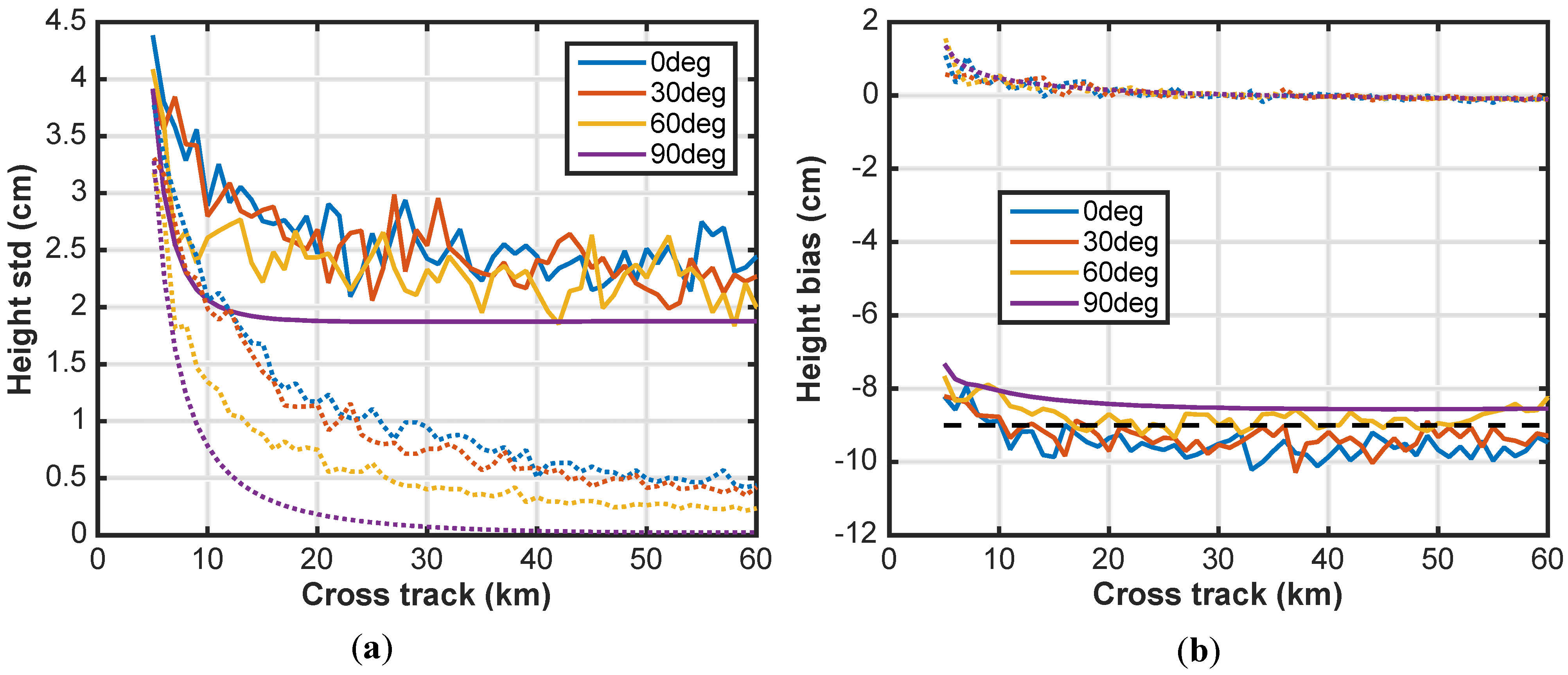
Figure 5 shows the height error, both standard deviation (a) and bias (b), as a function of cross track for SWH = 3 m for four different wave directions, where 0 deg means that the wave is aligned with boresight, and 90 deg means that it is aligned in the along-track direction. The dotted curves correspond to no backscattering modulation. In this case, when the ocean wave is aligned with the cross track, the error increases as the inverse of ground range, as predicted by the first-order theory, whereas in the along-track direction it grows as the inverse of ground range squared, which is consistent with higher order effects. Even without backscattering modulation, there is some height bias associated with second order effects, which increases in the near range and for large waves. The backscattering modulation has a first order contribution that is nearly constant across the swath, both for the height standard deviation and the height bias. The dashed black line in Figure 5b corresponds to the theoretical value from Equation (9). Deviations from that in the far range are mostly due to the impact of the tilt modulation.

Figure 5. Height standard deviation (a) and mean bias (b) for a 3 m SWH unidirectional ocean wave field with the Pierson-Moskowitz spectrum for various directions relative to the boresight (0 deg is aligned with boresight, 90 deg is in the along-track direction) computed using radar simulations for the SWOT geometry, radar parameters, and on board radar processing. Solid is for $\beta =3\%$ and tilt modulation, and dotted is for no backscattering modulation. The dashed black line in (b) corresponds to the theoretical EM bias in Equation (9).

Figure 5. Height standard deviation (a) and mean bias (b) for a 3 m SWH unidirectional ocean wave field with the Pierson-Moskowitz spectrum for various directions relative to the boresight (0 deg is aligned with boresight, 90 deg is in the along-track direction) computed using radar simulations for the SWOT geometry, radar parameters, and on board radar processing. Solid is for $\beta =3\%$ and tilt modulation, and dotted is for no backscattering modulation. The dashed black line in (b) corresponds to the theoretical EM bias in Equation (9).

5. WAVEWATCH-III Simulation Results

The error associated with the surfboard sampling effect is highly dependent on the ocean wave spectrum; not only its magnitude, but also its orientation and peak wavelength, and a one-dimensional Pierson-Moskowitz spectrum is not a sufficiently realistic representation of actual wave spectra, including swell traveling in directions not aligned with the wind direction. In order to quantify the impact of the waves on the projected SWOT performance, we have used a relatively large number (~300) of uniformly distributed locations on the globe for which WAVEWATCH-III global model spectra are available, and simulated the height error at different times of the year, corresponding to various conditions of SWH and wave energy distribution, for a total of ~1200 spectra. Each of these includes simulation of 25 different wave realizations of the spectrum. Since the wave direction is not isotropic across the globe, the predicted on-orbit spacecraft heading relative to the waves at that location has been used for each spectrum. In these simulations, we include the hydrodynamic modulation with $\beta =3\%$ and the tilt modulation.

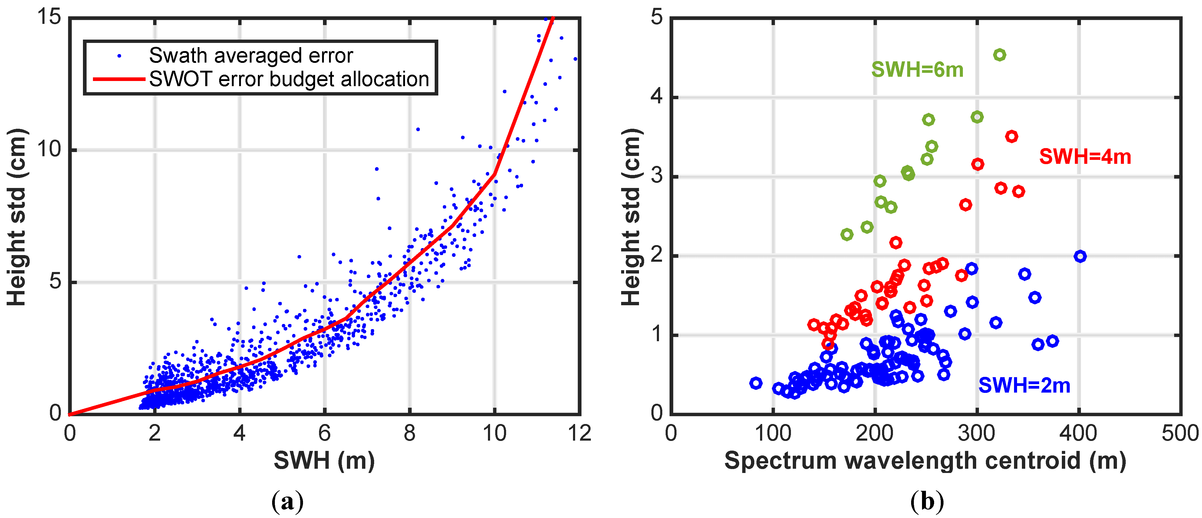
Figure 6a illustrates the RMS over the nominal swath from 10 km to 60 km of the height standard deviation as a function of SWH. As a comparison, the red curve indicates the height error as a function of SWH that is used to project SWOT performance, which is computed as the mean variance for each SWH. As in Section 4, this height error only presents the systematic error component, and does not include any increase in random error due to decreased coherence. These results also incorporate the error due to wave aliasing, although this is a small fraction of the total error, which is largely dominated by the surfboard and backscattering modulation. By comparing the results of Figure 5a with Figure 6a, it is evident that the unidirectional wave spectrum is highly pessimistic, and statistically the height error averages down to a smaller value for a two-dimensional wave scene.

The spread in values for the error at a particular SWH that Figure 6a exhibits is due to the fact that the error is highly dependent on the spectral distribution of the wave field, both in frequency and space. We have found that the error is particularly correlated with the spectrum wavelength centroid, as illustrated in Figure 6b, since more energy around the centroid is transferred on to longer wavelengths, thus corrupting the 1km x 1km pixels.

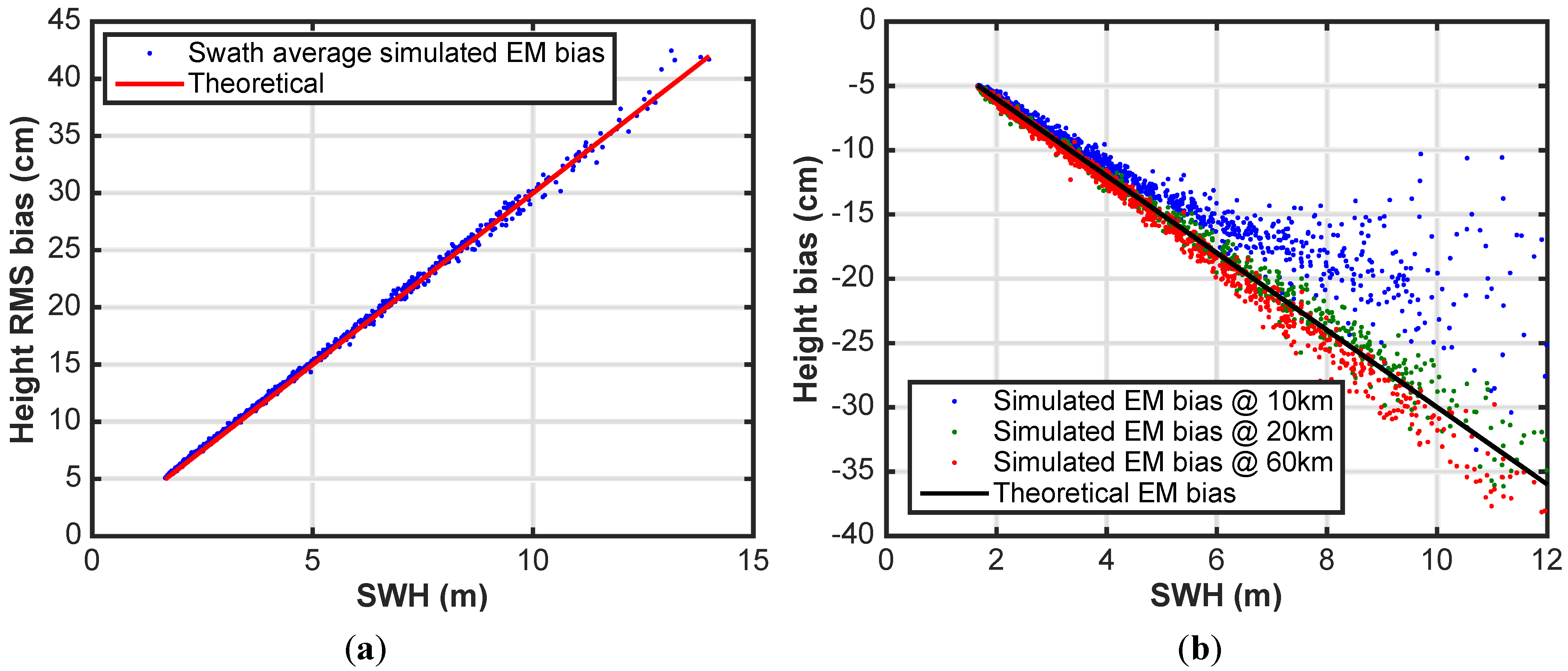
The first order theory in the Appendix predicts that the electromagnetic bias, $\langle h_m\rangle$, is not impacted by the surfboard sampling, and that it follows the expression $\langle h_m\rangle =\langle h\delta \sigma \rangle$. For $\delta \sigma =-4\beta \frac{h}{{\sigma }_h}$, as assumed in the simulations, the result is $\langle h_m\rangle =-\beta \cdot SWH$. Figure 7a shows the simulated RMS over the swath of the height bias as a function of SWH (in blue), which is roughly approximated by the results predicted by the first order theory (in red). However, this theory is not valid in the near range, as shown in see Figure 7b, which displays the height bias as a function of SWH for three different ground ranges, 10 km (blue), 20 km (green) and 60 km (red). The solid black line corresponds to the theoretical bias. Beyond 20 km, the height error is fairly well represented by the theoretical expression.

Figure 6. (a) Swath average height error for 1 km × 1 km pixels as a function of SWH for multiple WAVEWATCH-III spectra. The red curve is the height error as a function of SWH that is used to project SWOT performance. (b) Swath average height error for 1 km x 1 km pixels as a function of the spectrum wavelength centroid.

Figure 6. (a) Swath average height error for 1 km × 1 km pixels as a function of SWH for multiple WAVEWATCH-III spectra. The red curve is the height error as a function of SWH that is used to project SWOT performance. (b) Swath average height error for 1 km x 1 km pixels as a function of the spectrum wavelength centroid.

Figure 7. (a) Swath average electromagnetic bias as a function of SWH (blue), compared with the first order theory (red). (b) Electromagnetic bias at 10 km (blue), 20 km (green) and 60 km (red) as a function of SWH, compared with Equation (9) in black. Note the positive slope in (a) is due to the fact that the RMS value is computed.

Figure 7. (a) Swath average electromagnetic bias as a function of SWH (blue), compared with the first order theory (red). (b) Electromagnetic bias at 10 km (blue), 20 km (green) and 60 km (red) as a function of SWH, compared with Equation (9) in black. Note the positive slope in (a) is due to the fact that the RMS value is computed.

6. Impact of Surface Waves on Projected SWOT Performance

Ocean waves degrade the projected performance of the proposed SWOT mission, especially in the near range. This is not a phenomenon unique to radar interferometry, and altimeter performance has also been shown to be impacted by waves [29]. The height variance, ${\sigma }_{h_m}^2$, due to the surface waves (not including volumetric decorrelation) can be modeled as a function of ground range, $x$, as a constant term, $C_{{\sigma }_0}$, which is due to the backscatter modulation, and as a term that varies as the inverse of the ground range squared, which is attributed to the surfboard as follows:

$${\sigma }_{h_m}^2=C_{{\sigma }_0}+\frac{C_{SF}}{x^2}$$

(10)

The two coefficients, $C_{{\sigma }_0}$ and $C_{SF}$, have been derived as a function of SWH by fitting the simulated WAVEWATCH-III data presented in Section 5, and are plotted in Figure 8a. Equation (10) agrees with the conclusions of the first order theory included in the Appendix (see Equation (23)).

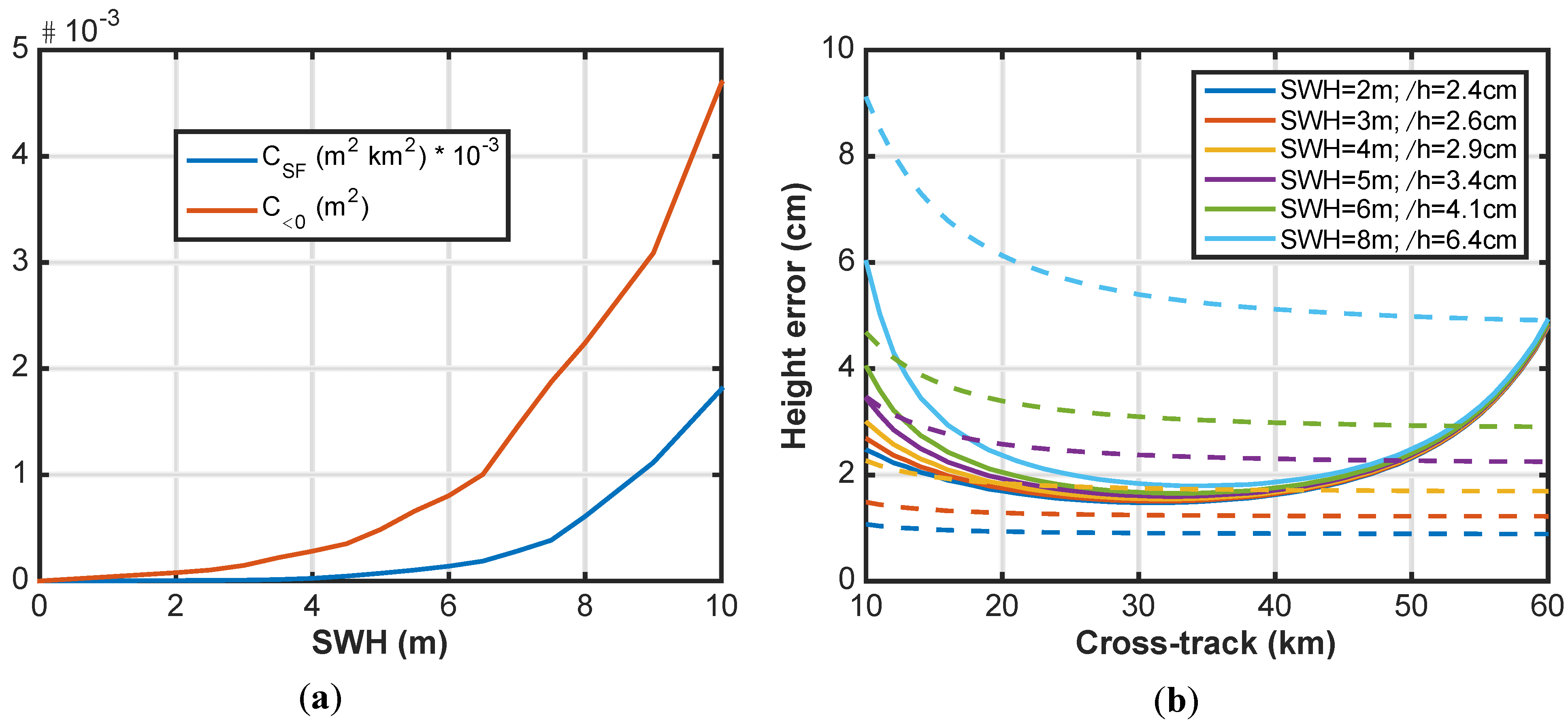
Figure 8b compares the height error due to random effects (thermal, volumetric decorrelation due to waves, geometric and angular decorrelation, and pointing errors [1]) to the systematic error due to waves (wave aliasing, surfboard and backscattering modulation), which follows Equation (10). SWOT’s performance requirement is specified for a SWH of 2 m, which is identical to what has been traditionally imposed on the Jason series of nadir altimeters. For that SWH, the systematic height error due to the ocean waves is small (2.4 cm swath average total error, compared to 2.2 cm without including the surfboard and backscattering modulation), but as the wave energy increases, the error due to the waves becomes a significant portion of the total height error. Indeed, for SWH larger than 4 m, the surfboard and backscattering modulation become the dominant error source.

Figure 8. (a) Coefficients that best fit the WAVEWATCH-III results for height variance versus cross track distance, according to Equation (10) (b) Height error for 1 km × 1 km pixels as a function of cross track due to random noise (solid) and the nonlinear wave energy transfer (dotted) for several SWH. The legend indicates the swath average height error for each SWH.

Figure 8. (a) Coefficients that best fit the WAVEWATCH-III results for height variance versus cross track distance, according to Equation (10) (b) Height error for 1 km × 1 km pixels as a function of cross track due to random noise (solid) and the nonlinear wave energy transfer (dotted) for several SWH. The legend indicates the swath average height error for each SWH.

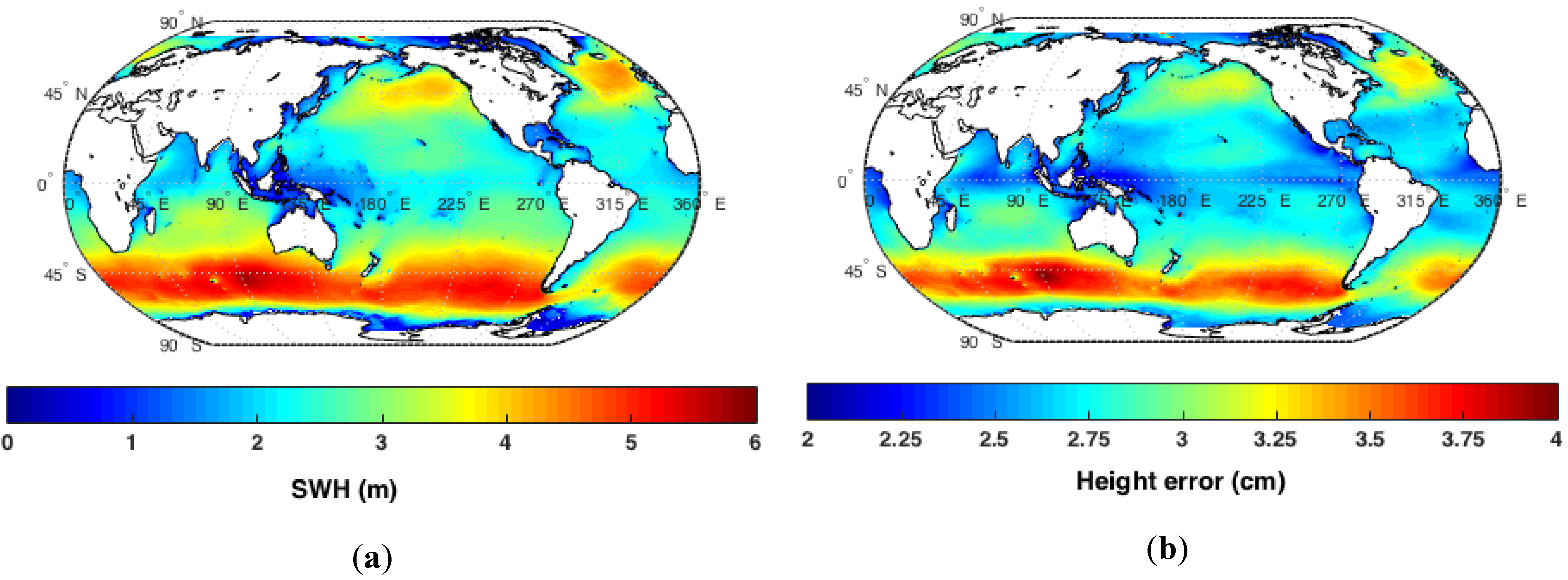
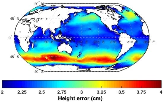
The global distribution of SWH indicates that SWH is less than 2.5 m with 50% probability, and roughly 3 m with 68% probability (1-sigma). However, locally the SWH can be significantly higher, as illustrated in Figure 9a, which shows a geographical map of the 1-sigma value for SWH obtained from one year of WAVEWATCH-III simulated data. The predicted swath average height error for SWOT for 1 km × 1 km pixels is shown in Figure 9b using the local 1-sigma values for SWH and windspeed, which is related to sigma-0. It is evident that, in some regions of the globe, the projected SWOT performance will be degraded relative to the performance specified for a SWH of 2 m or, equivalently, the effective swath with a certain level of performance will be reduced.

Figure 9. (a) Significant Wave Height (SWH) 1 sigma (68%) value based on one year of WAVEWATCH-III simulations. (b) Swath average height error for 1 km × 1 km pixels.

Figure 9. (a) Significant Wave Height (SWH) 1 sigma (68%) value based on one year of WAVEWATCH-III simulations. (b) Swath average height error for 1 km × 1 km pixels.

7. Conclusions and Future Work

We have presented the various phenomena related to surface waves that degrade the projected performance of the proposed SWOT mission. The wave volumetric decorrelation introduces a random error, which is destructive and cannot be corrected. The other error sources (aliasing, surfboard, and backscattering modulation) are systematic in nature, and knowledge of the wave fields and the backscatter both in phase and magnitude would allow partial error mitigation. However, due to the temporal and spatial variability of the waves, the error appears as random and can only be characterized in a stochastic sense. The only correction that can be applied in practice is the average electromagnetic bias. An estimate of the electromagnetic bias could potentially be made with higher accuracy by applying some knowledge of the wave spectrum.

It has been shown that the errors are significant for large waves, and this will impact the accuracy of SWOT’s measurements, especially in some regions like the Southern Ocean. It has also been shown that SWOT’s projected performance depends on parameters, such as the hydrodynamic modulation, for which there are not many measurements. Future work will include validation of the results using AirSWOT, an aircraft validation/calibration platform that is currently under development by the SWOT mission.

Future work will also demonstrate that a similar analysis to that presented in the Appendix is valid for radial velocity, and the analytical formulation for the errors due to the surfboard and the backscattering modulation will be expanded to include higher order effects.