Article

Using RPAS Multi-Spectral Imagery to Characterise Vigour, Leaf Development, Yield Components and Berry Composition Variability within a Vineyard

1
Instituto de Ciencias de la Vid y del Vino (University of La Rioja, CSIC, Gobierno de La Rioja), Finca La Grajera, Carretera de Burgos Km 6, Logroño 26007, Spain
2
Instituto de Economía, Geografía y Demografía. Centro de Ciencias Humanas y Sociales, CSIC, Albasanz 26–28, Madrid 28037, Spain
3
Institute of Earth Sciences Jaume Almera, ICTJA-CSIC, Lluis Sole Sabaris s/n, Barcelona 08028, Spain
*
Author to whom correspondence should be addressed.
Remote Sens. 2015, 7(11), 14458-14481; https://doi.org/10.3390/rs71114458
Submission received: 1 September 2015 / Revised: 30 September 2015 / Accepted: 26 October 2015 / Published: 30 October 2015
(This article belongs to the Special Issue Remote Sensing in Precision Agriculture)

Abstract

:
Implementation of precision viticulture techniques requires the use of emerging sensing technologies to assess the vineyard spatial variability. This work shows the capability of multispectral imagery acquired from a remotely piloted aerial system (RPAS), and the derived spectral indices to assess the vegetative, productive, and berry composition spatial variability within a vineyard (Vitis vinifera L.). Multi-spectral imagery of 17 cm spatial resolution was acquired using a RPAS. Classical vegetation spectral indices and two newly defined normalised indices, NVI1 = (R802 − R531)/(R802 + R531) and NVI2 = (R802 − R570)/(R802 + R570), were computed. Their spatial distribution and relationships with grapevine vegetative, yield, and berry composition parameters were studied. Most of the spectral indices and field data varied spatially within the vineyard, as showed through the variogram parameters. While the correlations were significant but moderate among the spectral indices and the field variables, the kappa index showed that the spatial pattern of the spectral indices agreed with that of the vegetative variables (0.38–0.70) and mean cluster weight (0.40). These results proved the utility of the multi-spectral imagery acquired from a RPAS to delineate homogeneous zones within the vineyard, allowing the grapegrower to carry out a specific management of each subarea.

Graphical Abstract

1. Introduction

Modern and sustainable viticulture requires objective and continuous monitoring of key parameters for rational and differentiated agronomic management of vineyards based on the spatio-temporal variability of growth, yield, and grape composition within the plot. The differential management within the vineyard and the concept of being spatially variable are covered by a discipline known as precision viticulture. This new approach allows the grape-grower to optimize crop production and profitability by reducing inputs such as machinery, labour, chemicals, water, energy, etc. It also contributes to diminishing the environmental impact of pesticides, nutrients leaching, and fossil fuels, among others [1,2].
One of the tools that has demonstrated its capability to help in crop management, and more specifically, in studying the within-field variability to assess spatial and temporal changes in soil moisture, canopy growth, and plant water status, is remote sensing. Several works have shown the suitability of remote sensing for precision viticulture purposes during the last two decades [3]. Hence, this technique has been used to appraise the vineyard spatial variability of water status [4,5], chlorophyll and carotenoid content [6,7], vineyard canopy structure [8,9], grape colour and phenols content [10,11], as well as grape quality [6,12]. Remote sensing involves the acquisition of spectral data from several platforms, such as satellites, aircrafts, and remotely piloted aerial systems (RPAS).
Vineyards are not a continuous crop, unlike cereals. Thus, spectral mixing between individual vines and row soil background is one of the main drawbacks for operational application of remote sensing data to vineyard monitoring [13]. Even for very high-resolution space borne sensors such as Pleiades Constellation (http://smsc.cnes.fr/PLEIADES/), the highest spatial resolution available is 50 cm/pixel, which could still be too coarse to monitor some common vine training systems where crop canopies are very narrow (i.e., 40–60 cm in the case of vertical shoot positioned vineyards), and a mixed signal of leaves, shoots, shadow, and soil is commonly found in most pixels. Sensors on board manned airborne vehicles allow these limitations to be overcome by acquiring imagery of increased spectral, spatial, and temporal resolution compared to those mounted on satellites, although their operational costs are very high. RPAS is an interesting alternative in precision viticulture to other platforms such as helicopters, airborne, and satellite, regarding mainly the spatial resolution and the cost of acquisition [14]. RPAS allow for the acquisition of imagery of very high spatial resolution, often at a sub-decimetre resolution, at much lower cost than traditional airborne remote sensing. Furthermore, it has been proven that results obtained from a RPAS for agricultural application may yield similar estimations in terms of accuracy and precision to those derived from traditional airborne platforms [15]. These facts, together with their lower cost and higher temporal flexibility, explain the increased use of RPAS for agricultural purposes [16]. As a matter of fact, a very recent report on the economic impact of unmanned aircrafts in the United States (US) [17] revealed that the use of RPAS in agriculture in 2015 in the US would yield $2096.5 and an expected creation of 21,565 jobs. Among the applications of RPAS in viticulture, the assessment of within-vineyard variability stands out [18], as the spatial and temporal resolutions are key attributes when the goal of the study is monitoring and managing the vineyard [3].
Most of the remote sensing studies in agriculture are based on the use of spectral indices. These are arithmetical combinations of the original spectral bands captured by the sensor, which reduce the complexity of the dataset [3] and facilitate the analysis of various vegetation parameters that are directly related to their spectral response at given wavelengths. Vegetation indices, like the normalised difference vegetation index (NDVI), have been extensively used to monitor crop status by relating visible and near infrared spectral data with bio-geophysical properties of the vines such as vigour and leaf area [18]. Other spectral indices like the photochemical reflectance index (PRI) combine information from two narrow bands in the visible region to monitor vegetation stress [19].
The present work aims to show the capability of multispectral imagery acquired from a RPAS, and the derived spectral indices, to assess and map the spatial variability of vegetative and yield components, as well as berry composition in a vineyard (Vitis vinifera L.) for precision viticulture management.

2. Materials and Methods
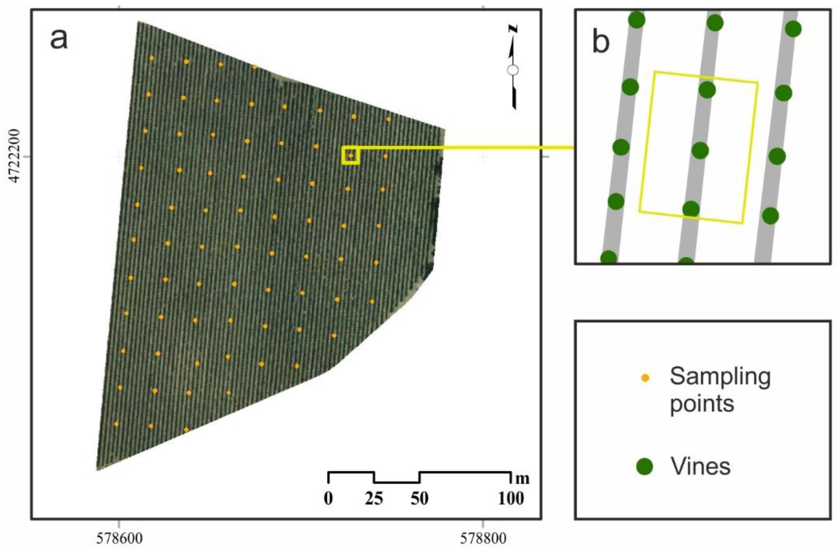
2.1. Study Area

The study was conducted in a 3.0 ha Tempranillo (Vitis vinifera L.) vineyard located in Navarra, Spain (Figure 1). Grapevines were planted in 2004 in a sandy-clay soil (5% slope towards North), using a 41B rootstock at 2.4 m × 1.6 m (inter- and intra-row) with north-south row orientation. Vines were trained to a vertically shoot-positioned (VSP), spur-pruned cordon retaining 16 nodes per linear meter/vine. Vines were uniformly irrigated twice across the season.
Figure 1. Experimental Tempranillo vineyard plot with the 72 sampling points (a). Schematic describing the position of the three adjacent vines comprising a sampling point (b).
Remotesensing 07 14458 g001

2.2. Field Data Acquisition of Vegetative and Yield Components. Berry Composition Analysis.

A regular grid of 72 sampling points at 20 m intervals was generated within the vineyard using a Leica Zeno 10 GPS (Heerbrug, St. Gallen, Switzerland), with real-time kinematic correction, working at <0.4 m precision. Each sampling point consisted of three adjacent vines (Figure 1b). Vegetative and yield-related data were measured in the field from all sampling points. As indicators of vine vigour, main and secondary shoot length and pruning weight were measured. Regarding vigour-related variables, main and secondary leaf area per shoot were determined. Secondary shoot length and secondary leaf area per shoot were measured for the three vines included in each sampling point one week prior to the RPAS flight, on 13 September 2011. For each vine, two shoots were randomly chosen and their main shoot length, as well as those of laterals with more than three leaves, were measured using a meter tape [20]. Main and secondary leaf area per shoot were estimated by defoliating each shoot and weighing the leaves with a portable scale of precision ±2 g (Kern and Sohn GmbH, Balingen-Frommern, Germany), using the disc-leaf method by Smart and Robinson [21]. The pruning weight of each vine was manually determined in the field using a hanging scale two months after the flight, on 20 November 2011, prior to vine pruning. Additionally, non-destructive measurement of photosynthetic pigments in plants were obtained on 13 September 2011, using a Multiplex™ (Multiplex 3.0, Force-A, Orsay, France), a handheld fluorescence-based proximal sensor that allows the computation of fluorescence-based indices related to the chlorophyll content in leaves (SFR_RAD) and the nitrogen balance index (NBI_GAD). The Multiplex™ sensor used for this study was a modified version of the device recently described by Ben Ghozlen et al. [22]. Multiplex™ measurements were performed on three main leaves (adaxial side) per sampled vine. From these measurements, the fluorescence indices were calculated as follows:
S F R _ R A D   =   F R F _ R A D R F _ R A D
N B I _ G A D   =   F R F _ U V A D R F _ G A D
where FRF_R and FRF_UV refer to the far red fluorescence emission excited by red and UV light, respectively, and RF_R and RF_G refer to red fluorescence excited by red light and green light, respectively [23]. The subscript AD stands for the adaxial side of the leaf. SFR_RAD has been reported as a precise indicator of the chlorophyll content in kiwi leaves [24] and in grapevine leaves [25], and NBI_GAD has also been shown as a reliable indicator of the nitrogen status of the grapevine [25].
At harvest time (17 October 2011), main yield components, such as cluster number per vine, yield per vine, cluster weight, and berry weight, were determined for each sampled vine. Each plant was manually harvested, their clusters counted and weighed in the vineyard using a hanging scale, and the average cluster weight calculated. Two clusters per vine were then labelled, kept apart and taken to the laboratory of the University of La Rioja in portable refrigerators where they were manually destemmed. Berries from each cluster were weighed (TE3102S, Sartorius, Goettingen, Germany) and counted, and the average berry weight calculated.
To determine berry composition, from the berries corresponding to each vine, a representative subsample of 50 berries was taken and weighted. These berry subsamples were then stored frozen at −20 °C until colour and phenolic analyses. The remaining berries of each vine were pressed and the obtained must was analysed for total soluble solids concentration (TSS) and acidity parameters. TSS (expressed in Brix) was determined using a temperature-compensating digital refractometer (Atago, Tokyo, Japan), while titratable acidity and pH were determined following the OIV methods [26]. Anthocyanins and total phenols were analysed for each berry sub-sample applying the method of Iland et al. [27]. Anthocyanin concentrations were expressed as mg/g of fresh berry mass, whereas total phenols were expressed as absorbance units (AU) at 280 nm/g of fresh berry mass.
For all data collected in the field and relative to berry composition, the values of the three vines per sampling point were averaged and a mean value was then assigned to each sampling location. The vegetative variables, pruning weight, main leaf area and secondary leaf area, and the productive variable, yield, were transformed to surface units (per m2) by dividing them by the vine spacing [28].

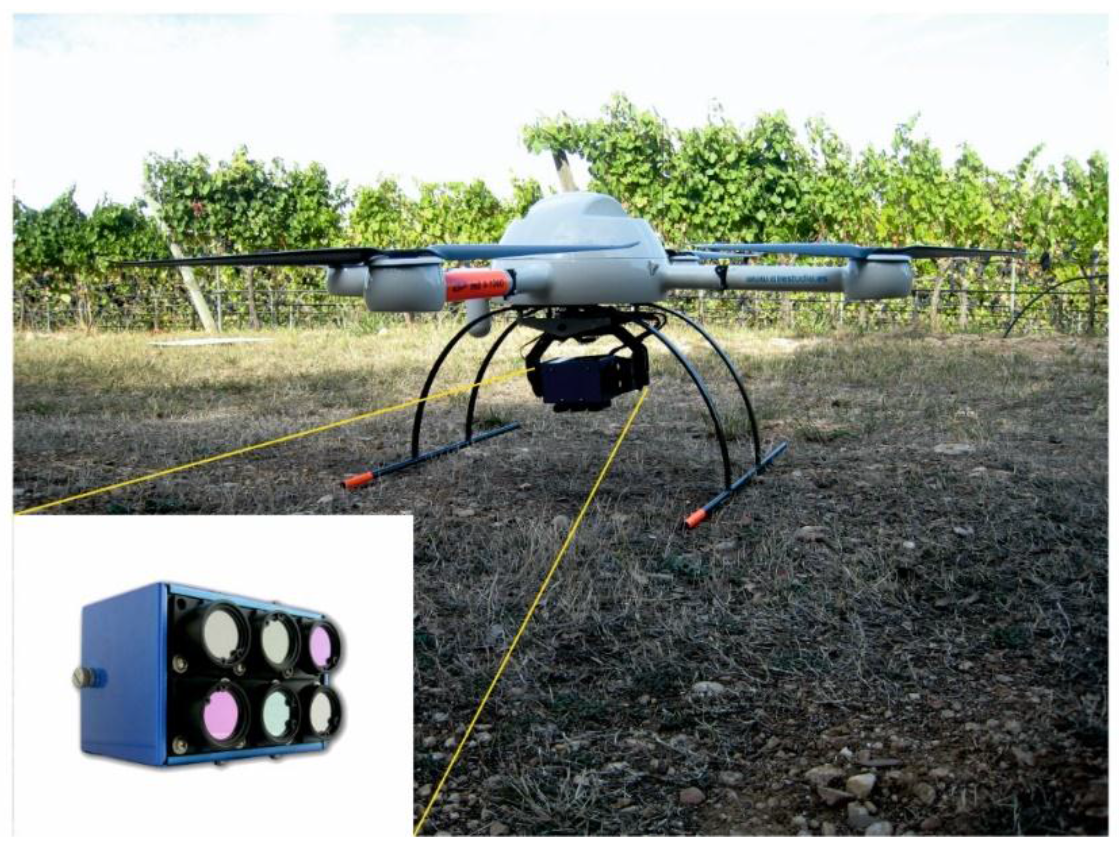
2.3. RPAS Multi-Spectral Images

Multi-spectral imagery was acquired with a multi-spectral camera, a mini multiple camera array (MCA 6, Tetracam Inc, Chatsworth, CA, USA) mounted on a RPAS Md4-1000 (Microdrones GmbH, Siegen, Germany) on 20 September 2011 (Figure 2). The RPAS Md4-1000 is a quadrotor able to carry 1.2 kg of payload mass and able to fly up to 88 minutes, with vertical take-off and landing. The camera consisted of six independent image sensors and optics with user-configurable filters. Image resolution was 1280 × 1024 pixels with 10-bit radiometric resolution and optics focal length of 9.6 mm. For this study, the camera was equipped with six 25 mm-diameter bandpass filters of 10 nm full-width at half-maximum (FWHM) (Andover Corporation, NH, U.S.), with centre wavelengths at 531, 551, 570, 672, 701, and 802 nm, and bandwidth of ±9.31, 10.13, 9.29, 9.82, 9.47, and 10.11 nm, respectively. The wavebands were selected in order to obtain the spectral bands required for the calculation of the spectral indices commonly used in agriculture, and, specifically, viticulture-related literature.
Figure 2. Multispectral camera mounted on the RPAS Md4-1000 and detail of the multiple camera array.
Remotesensing 07 14458 g002
The RPAS flew at 250 m height and allowed capturing images with a spatial resolution of 17 cm. Images were taken at noon, between 11:15 a.m. and 12:15 p.m., under stable weather conditions and clear sky (mean wind velocity of 1.39 m/s). At this time, grape berries were at the half-way point of their ripening process. A total of 6 scenes were acquired (with an overlapping area of 60%) in order to monitor the whole vineyard plot lengthwise. Each image covered a ground surface of approximately 200 × 165 m. It was able to cover the whole plot with one flight due to the reduced extension of the vineyard, the flying height, and the camera weight (700 g), which allowed the RPAS to have enough flight operational time.

2.4. Image Processing

From the 6 overlapping images obtained with the multi-spectral camera, two scenes that covered the whole vineyard plot were selected for the present study. An initial pre-processing of the images acquired with the Mini MCA camera was carried out using its companion application Pixel Wrench 2 (PW2), written and copyrighted by Tetracam Inc., to produce multi-page Tagged Image Format (TIF) files. As the multi-spectral camera uses six different lenses (one for each spectral band), it is necessary to confirm that the bands are aligned among them. Band alignment is important to ensure consistent spectral information, but when this correction is carried out by PW2, it turns out to be insufficient according to Laliberte et al. [29]. In agreement with these findings, the results of the inter-band alignment performed with PW2 showed substantial errors in this study and, therefore, it was decided to skip the alignment processed included in PW2 by setting a null aligning matrix and carry out a specific correction. Band alignment was performed by applying the Fine Registration algorithm of the Orfeo Toolbox [30] by using a reference band (band 2). This process calculates the local shifts in the x and y directions that result in the best local correlation between the band to be processed and the reference band, and creates a deformation field that is subsequently applied to the band to be processed. After a set of tests with a range of radii, the local windows to explore and calculate correlations were set to 5 × 5 pixels for bands 1, 3 and 4, and 7 × 7 pixels for bands 5 and 6. In addition, as the displacement with respect to the reference band was larger for bands 5 and 6, a rigid translation was applied in both x and y directions prior to the fine registration processing for these two bands.
Once the band alignment corrections were completed, the images were georeferenced to allow for the correlation of image data with field measurements. This was done by using cartographic co-ordinates from eight reference targets (white discs of 30 cm of diameter) located at the boundaries of the vineyard plot. Those targets had been georeferenced in the field during image acquisition using a Leica Zeno 10 Global Positioning System (GPS) (Heerbrug, St. Gallen, Switzerland). An orthophoto of the area of study provided by the Spanish National Program of Aerial Ortophotography (PNOA) with 25 cm spatial resolution was complementarily used to identify 45 ground control points in each scene. These points were evenly distributed over the image area including the borders, where displacement errors were higher because of the larger distance from the image nadir. A second degree polynomial function was applied using a bilinear resampling method to render the geometrically corrected image. Image georeferencing was carried out with an accuracy of 0.62 and 0.35 m (root mean squared error). Interactive location of ground control points, polynomial fit, and interpolation were performed using ENVI 4.8 (Exelis, McLean, VA, USA).
Radiometric calibration was performed using an image of a white calibration panel that was acquired from the ground with the mini MCA (at a distance about 1.5 m) prior to the flight. A reflectance spectrum of the same panel was measured at the Environmental Remote Sensing and Spectroscopy Laboratory (SpecLab) using an ASDFieldSpec 3 spectroradiometer (ASD Inc., Boulder, CO, USA). Image DN (Digital Numbers) from the calibration panel measured in the field were averaged for each band to calculate the observed reference DN spectrum. The reflectance spectrum measured in the laboratory was integrated to calculate the theoretical reflectance values of the panel for each mini MCA band using the transmission curves of the filters (www.andovercorp.com). A vector of factors was computed to transform the observed DN spectrum of the image into the modelled reflectance spectrum. These factors were then applied to each band of the image in order to obtain calibrated reflectance for each image pixel. Images were calibrated to apparent reflectance, i.e., reflectance as if the camera had been operated at 1.5 m. Atmospheric correction was not performed, but as the area was small and the atmospheric conditions very clear, the uniform atmospheric effect eventually present in the indices was taken into account by the linear models between indices and field data. The radiometric calibration operations were conducted by means of specific functions written in R Core Team [31] and using packages rgdal [32] and raster [33].
The next step was the spatial assembly of the images to build the final mosaic, so the whole vineyard plot fit within a single image file. The mosaicking process was performed using ENVI (Exelis Visual Information Solutions, Inc, Boulder, CO, USA) software by combining the two scenes that included the whole vineyard. We assigned, as base image, the scene that covered most of the plot, so the colour balance in the second image was carried out to match the base image by using histogram matching. A distance of 40 pixels was set to blend the two images.
Using the corrected image mosaic, a total of 11 spectral indices, selected from the literature as being the most commonly used to characterise vegetation status, were calculated (Table 1 [34,35,36,37,38,39,40,41,42]). These indices have been proposed to estimate a wide variety of vegetation properties including pigment contents, leaf area index, plant health status, nutrient stress, etc., and some of them have been widely used in precision viticulture. Some indices specially designed to minimize the effects of soil background on the vegetation signal as the OSAVI and MSAVI were also included in the analysis.
In addition to these indices, a set of normalised indices were calculated as all possible-combinations between every image band, following the equation:
N o r m a l i s e d   i n d e x =   B a n d 1 B a n d 2 B a n d 1 + B a n d 2

2.5. Statistical Analysis

With the aim of establishing an empirical relationship between image data and field measurements, image pixels corresponding to the 72 sampling points were identified. For each sampling point, the two most centred pixels (6 pixels per point) were selected. Image values were extracted from those pixels, the spectral indices were computed and averaged per sampling point for each band. Prior to the statistical analysis, the data were pre-processed in order to detect potential outliers.
Descriptive statistics were computed for all variables (mean, minimum, maximum, standard deviation and coefficient of variation), as well as the spread (Equation (4)), expressed in percentage, as an indicator of the variability in the sample [43].
S p r e a d =   ( m a x i m u m m i n i m u m ) m e d i a n
To characterise the spatial variability of the various parameters within the vineyard, variograms for the variables were calculated by the R package “gstat” [44]. The parameters of the variograms were also used to interpolate all the variables, using kriging techniques.
Finally, to quantify the agreement between the maps obtained from the spectral indices and the ones derived from field variables, all the maps were classified in three zones corresponding to low, medium, and high values applying an iso-cluster unsupervised classification. Cross tabulation of the resulted classified maps between the spectral indices and the in-field variables was performed to measure the stability in the spatial patterns using the Kappa index following the equation proposed by Hudson and Ramm [45]. Statistical and spatial analysis were carried out using Microsoft Office Excel 2013 (Microsoft Corporation, Washington, USA), Statistica 9.0 (Stat Soft, Inc., Tulsa, OK, USA), and ArcGIS Desktop 10.3 (ESRI, Redlands, CA, USA).
Table 1. Spectral vegetation indices commonly used in viticulture studies.
Spectral IndexReference
Normalized Difference Vegetation Index (NDVI)(Rouse et al. 1974) [34]
N D V I =   R N I R R R E D R N I R + R R E D
Modified Simple Ratio (MSR)(Chen 1996) [35]
M S R =   ( R N I R R R E D 1 ) [ ( R N I R R R E D ) 0.5 + 1 ]
Modified Triangular Vegetation Index (MTVI1)(Haboudane et al. 2004) [36]
M T V I 1 = 1.2 × [ 1.2 × ( R 800 R 550 ) 2.5 × ( R 670 R 550 ) ]
Renormalized Difference Vegetation Index (RDVI)(Roujean and Breon 1995) [37]
RDVI =   R NIR R VIS R NIR + R VIS
Greenness Index (G)-
G =   R G R E E N R R E D
Modified SAVI (MSAVI)(Qi et al. 1994) [38]
M S A V I =   1 2   [ 2 × R 800 + 1 ( 2 × R 800 + 1 ) 2 8 × ( R 800 + R 670 ) ]
Optimized Soil Adjusted Vegetation Index (OSAVI)(Rondeaux et al. 1996) [39]
O S A V I   =   ( 1 + 0.16 ) ( R N I R R R E D ) ( R N I R + R R E D + 0.16 )
Modified Cab Absorption in Reflectance Index (MCARI)(Daughtry et al. 2000) [40]
M C A R I   = [ ( R 700 + R 670 ) 0.2 × ( R 700 R 550 ) ] × ( R 700 R 670 )
Transformed CARI (TCARI)(Haboudane et al. 2002) [41]
T C A R I   =   3 × [ ( R 700 R 670 ) 0.2 × ( R 700 R 550 ) × ( R 700 R 670 ) ]
TCARI/OSAVI(Haboudane et al. 2002) [41]
T C A R I / O S A V I   =   3 × [ ( R 700 R 670 ) 0.2 × ( R 700 R 550 ) × ( R 700 / R 670 ) ] ( 1 + 0.16 ) × R 800 R 670 R 800 + R 670 + 0.16
Plant Cell Density Index (PCD) or Ratio Vegetation Index (RVI)(Jordan 1969) [42]
P C D = R V I =   R N I R R R E D

3. Results and Discussion

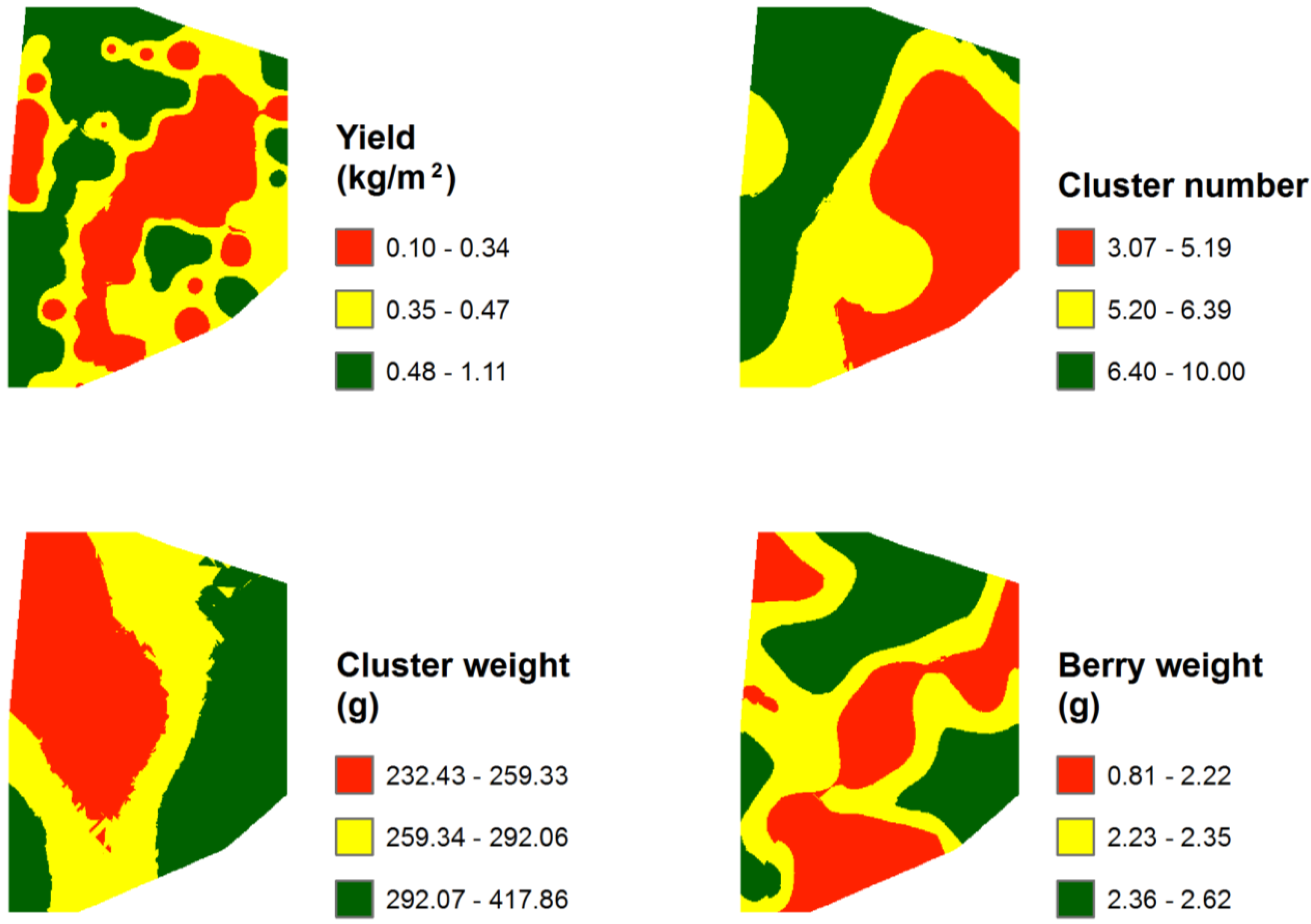
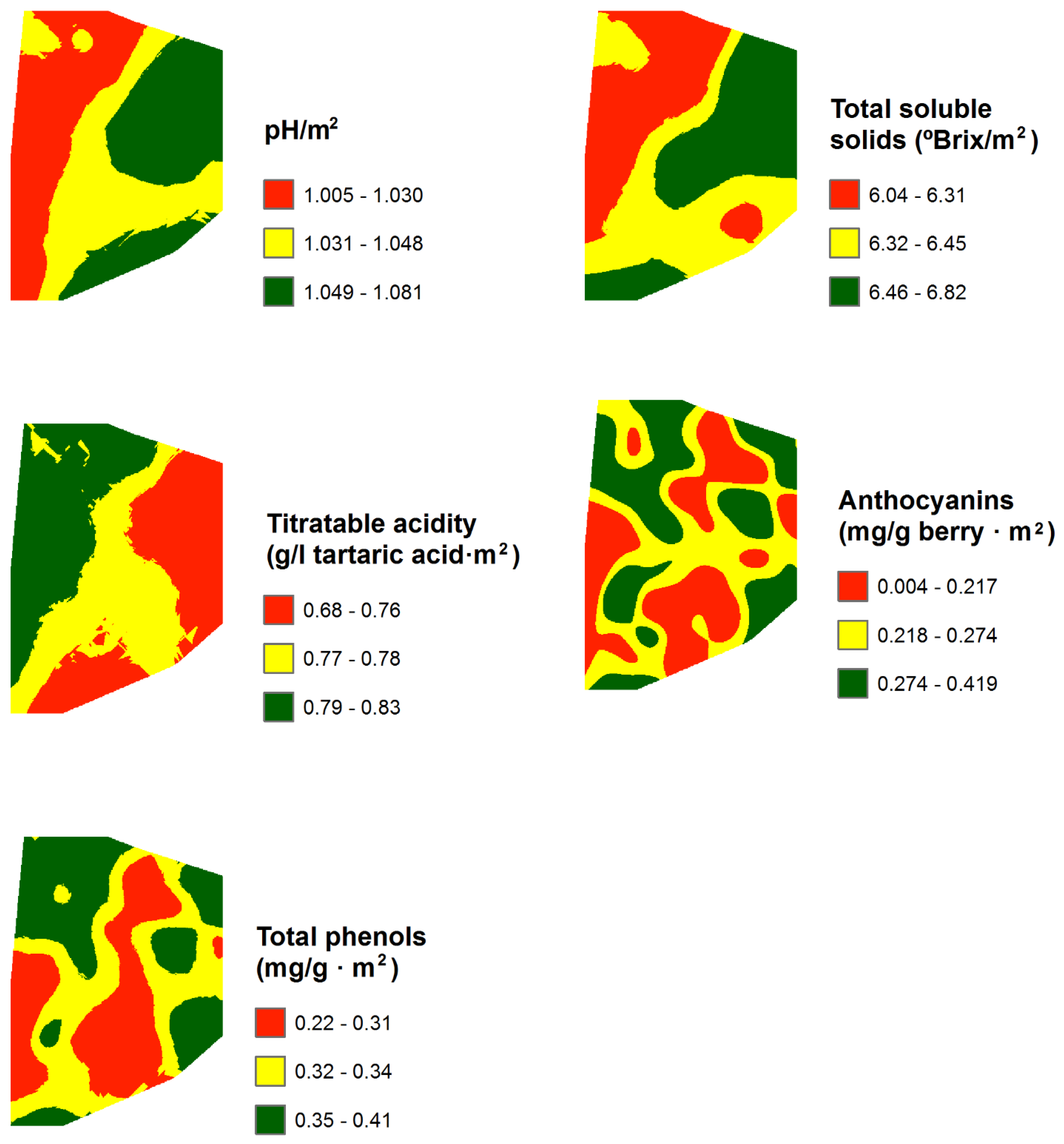
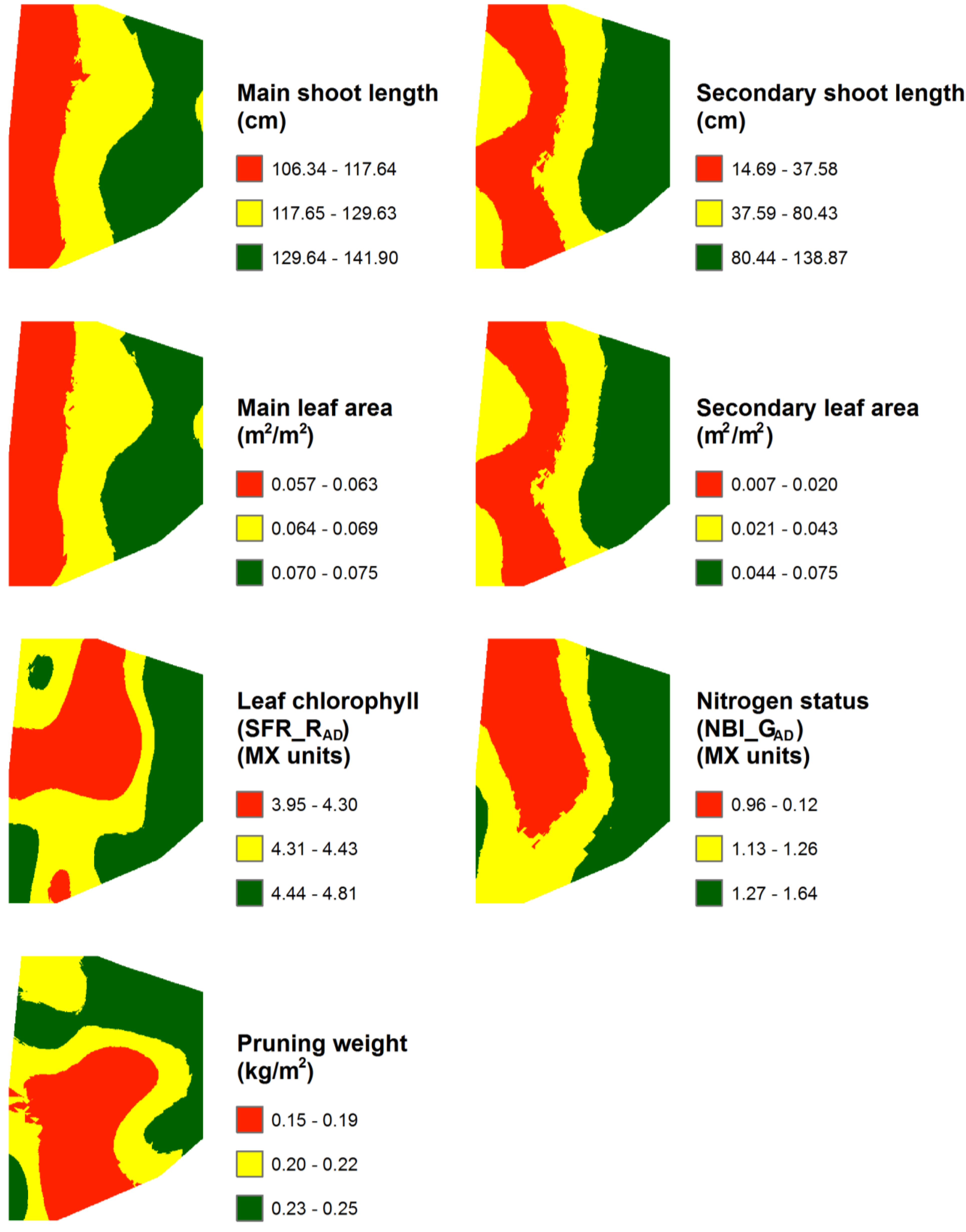
3.1. Spatial Variability of Spectral Indices, Field Variables, and Berry Composition

Spectral indices selected from literature (Table 1) and the normalised indices (Equation (3)) were correlated with field (ground truth) data in order to exclude from further analysis those indices that exhibited weak or not significant correlations. As a result, correlations with a Pearson coefficient, “r”, smaller than 0.35 in absolute value were discarded. Furthermore, the spectral indices with a high correlation coefficient were also discarded to avoid redundant information. The spectral indices that showed the lowest correlation were MTV1 or RDVI, which yielded mean correlation coefficients with in-field variables of around 0.2. The indices finally selected for further analysis were NDVI and G. Two indices from the group of normalised indices were also selected, which were named as Normalised Vegetation Index 1, NVI1 (R802 − R531/R802 + R531), and Normalised Vegetation Index 2, NVI2 (R802 − R570/R802 + R570), both resulting from the combination between NIR and green reflectance values, similar to the Green NDVI proposed by Gitelson et al. [46].
Descriptive statistics of the spectral indices and field variables are reported in Table 2. As it can be observed, most of them exhibited considerable variability within the vineyard. On the basis of coefficient of variation (CV) and Spread parameters, secondary shoot length and secondary leaf area were, by far, the field variables showing the largest variability (CV = 80%, Spread > 370%), followed by yield per vine (CV = 57%, Spread = 280%), and number of clusters per vine (CV = 51%, Spread = 250%). These values were similar to those observed by Baluja et al. [47] in Tempranillo in La Rioja (Spain) and by Bramley and Lamb [48] and Bramley and Hamilton [49] in Australia, in other varieties. The fluorescence index indicative of leaf chlorophyll content (SFR_RAD), the normalised indices NVI1 and NVI2, berry weight, pH, TSS, and titratable acidity showed a CV smaller than 10%. NBI has been described as a good indicator of the nitrogen status of grapevine leaves [24,50,51]. Its calculation depends on the concentration of flavonoids and chlorophyll in the leaf, so its variability must be higher than that of chlorophyll and flavonoids alone [51]. Furthermore, the presence of water deficit due to very warm temperatures (the average of the month mean temperatures during the study year exceeded between 1.5 °C and 3.2 °C the value of the average of the historical series mean temperatures) and dryness (total rainfall from July to September was 30.9% of average historical rainfall in this period) as reported by the Navarra Government’s meteorological station of Estella, may have induced a weak mineralization of soil nitrogen, which in turn led to nitrogen deficiency on the leaves of the vines in some areas of the vineyard, hence contributing to the large variability observed for the NBI_GAD index.
All of the experimental variograms of the variables studied were fitted to a Spherical or Gaussian model, with the exception of yield per vine and the anthocyanin concentration, which showed an absence of spatial structure as also found by Cerovic et al. [52]. The range of the variogram is the distance at which the sill (maximum semivariance) is achieved and indicates whether the samples are spatially dependent (samples separated by distances closer than the range) or spatially independent (samples separated by distances larger than the range) [53]. The range value was variable for all parameters studied (Table 2). Main leaf area, main shoot length, pH, and titratable acidity showed a range around 125 m. The spectral index, G, was the variable with the highest range value (202 m). The lowest values of the range (from 38 to 65 m), that is the lowest distance of spatial dependence, were found for the fluorescence index related to leaf chlorophyll content, the vegetative variable pruning weight, the two normalised spectral indices NVI1 and NVI2, for berry weight, and for total phenols. Specifically, the range obtained for the pruning weight agrees with the one reported by Taylor and Bates [54] for the case of 3-vines-aggregation. Furthermore, the nugget effect, which is the discontinuity at the origin of the variogram (unexplained variance) usually related to the variability at distances lower than the sampling grid, yielded, in general, values higher than 25% of the total variance. This indicates a moderate spatial dependence [55] with the exception of the normalized indices NVI1 and NVI2, with strong spatial dependence. The range and percentage of nugget for the main shoot length was similar to that obtained by Baluja et al. [47]. Cerovic et al. [52] also reported a similar value of percentage of nugget for the NBI_GAD and for cluster number per vine.
Table 2. Descriptive statistics and variogram components for spectral indices (NDVI, G, NVI1, and NVI2), vegetative parameters (pruning weight, main shoot length, secondary shoot length, main leaf area per shoot, and secondary leaf area per shoot), fluorescence-based indices of nitrogen balance index (NBI_GAD), and chlorophyll content in leaves (SFR_RAD) for yield parameters (cluster number per vine, cluster weight, yield per vine, and berry weight) and for grape composition variables (pH, total soluble solids, titratable acidity, anthocyanins, and total phenols) in a Tempranillo (Vitis vinifera L.) vineyard.
MeanMin.Max.SDCV (%)Spread (%)% of NuggetRange
Spectral indices
NDVI0.650.510.760.0610.0138.1129111.41
G1.311.001.660.1511.6250.6928202.01
NVI10.630.510.720.057.4232.90759.15
NVI20.670.570.740.046.4525.821357.73
Vegetative variables
Pruning weight (kg/m2)0.200.120.340.0525.21116.967052.65
Main shoot length (cm)123.2295.83172.1715.3612.4761.4446126.33
Secondary shoot length (cm)63.956.67189.8349.9978.17379.6133105.14
Main leaf area (m2/m2)0.070.050.090.0112.8760.0046122.55
Secondary leaf area (m2/m2)0.030.0030.100.0383.80475.003498.91
Leaf chlorophyll - SFR_RAD(Mx units)4.373.555.040.357.9234.176665.00
Nitrogen status - NBI_GAD(Mx units)1.210.691.940.3226.89108.7043152.55
Yield variables
Cluster number/vine6.061.5014.003.1451.82250.006280.79
Cluster weight (g)284.28147.50520.0073.0125.68133.1544156.42
Yield/vine (kg/m2)0.440.101.110.2557.19279.95
Berry weight (g)2.291.842.910.229.4746.753448.82
Grape composition variables
pH3.993.634.290.143.4516.5353117.54
Total soluble solids (ºBrix)24.6122.0326.871.154.6719.735272.69
Titratable acidity (g/l tartaric acid)2.952.303.670.289.5746.9659137.22
Anthocyanins (mg/ g berry)0.950.381.500.2627.65120.33
Total phenols (AU/g berry)1.260.601.850.3023.7799.975238
SD: standard deviation; CV: coefficient of variation; % Nugget = (nugget/(sill + nugget)) × 100. AU: absorbance units.

3.2. Correlation Analysis between Spectral Indices, Field Variables, and Berry Composition

The relationships between the spectral indices with the field variables related to the vegetative status and the yield of the vineyard were first explored by the computation of the Pearson correlation coefficients (Table 3). The strength of the correlations was found to be variable, with “r” values ranging from 0.32 to 0.69, for p-value < 0.01, in agreement with those reported by other authors [47,56,57,58,59].
In general, for the vegetative variables, the best performance was observed for the normalised spectral indices, NVI1 and NVI2, with coefficient values higher than 0.5. From all the vegetative variables studied, pruning weight exhibited the highest “r” values, although quite similar to those for shoot length and leaf area parameters. Other authors [47,57,59] have also shown significant correlations between vegetation indices, such as the NDVI and pruning weight. Regarding the fluorescence-based indices, low to moderate positive correlations were observed between the spectral indices NVI1 and NVI2 with leaf chlorophyll content (SFR_RAD) and nitrogen status (NBI_GAD).
Regarding the yield variables, while the number of clusters and the yield did not show any significant correlation with the spectral indices, mean berry weight and mean cluster weight were significantly correlated with all the spectral indices. The strong positive correlation (r = 0.90) between yield per vine and the number of clusters per plant (Table 2), together with the lack of significance with cluster weight and very poor (r = 0.35) with berry weight, suggest that the number of clusters per vine was the key component in determining the final grape production per plant, at the expense of average berry and cluster weight. This is an interesting outcome, as the number of clusters per vine is directly impacted by bud fertility, which is determined at the flowering period in the previous season [60] (May–June 2010). The weather conditions in Spring 2010 at the vineyard of study (data from Navarra Government’s meteorological station of Estella) were characterised by intense rainfall (94.9% of average historical rainfall in these two months), low radiation, and cooler temperatures than mean historical values for this area (−1.9 °C in May and −0.6 °C in June), as shown above. These adverse conditions may have imparted stronger differences in bud fertility among the grapevines within the vineyard of study, leading to the greater variability described for the number of clusters per vine and the critical role of this yield component in final yield per vine. It may also explain the lack of significance of the correlations between yield and the vigour spectral indices derived from RPAS imagery, as the time period mainly influencing yield was Spring 2010, while Spring–Summer 2011 determined grapevine vigour.
Table 3. Pearson correlation coefficients (for p-value < 0.01) for vegetative parameters (pruning weight, main shoot length, secondary shoot length, main leaf area per shoot, secondary leaf area per shoot, nitrogen status –NBI_GAD-, and chlorophyll content in leaves –SFR_RAD-), yield parameters (cluster number per vine, cluster weight, yield per vine, and berry weight) and grape composition variables (pH, total soluble solids, titratable acidity, anthocyanins, and total phenols) with spectral indices (NDVI, G, NVI1, and NVI2) in a Tempranillo (Vitis vinifera L.) vineyard.
NDVIGNVI1NVI2SFR_RADNBI_GADPruning WeightMean Shoot LengthSecondary Shoot LengthMain Leaf AreaSecondary Leaf AreaCluster NumberCluster WeightYieldBerry WeightpHTotal Soluble Solids Titratabe AcidityAnthocyaninsTotal Phenols
NDVI1
G0.841
NVI10.810.541
NVI20.790.560.981
SFR_RAD0.37NS0.540.531
NBI_GAD0.430.320.580.560.581
Pruning weight0.550.360.580.58NS0.361
Mean shoot length0.490.540.340.32NSNSNS1
Secondary shoot length0.490.470.520.50NS0.520.320.611
Main leaf area0.490.530.350.33NSNSNS1.000.591
Secondary leaf area0.490.470.520.50NS0.520.330.611.000.591
Cluster numberNSNSNSNSNS−0.34NS−0.37−0.50−0.35−0.501
Cluster weight0.590.510.650.690.450.560.59NS0.45NS0.45NS1
YieldNSNSNSNSNSNS0.35NS−0.31NSNS0.90NS1
Berry weight0.410.330.380.42NSNS0.52NSNSNSNSNS0.450.351
pHNSNSNSNSNSNS−0.400.37NS0.37NS−0.44NS−0.53−0.441
Total soluble solids NSNSNSNSNSNSNSNSNSNSNSNSNSNSNS0.521
Titratable acidityNSNSNSNSNSNSNSNSNSNSNSNSNSNS0.32−0.62−0.581
AnthocyaninsNSNSNSNSNSNSNSNSNSNSNSNSNSNSNSNSNS−0.331
Total phenolsNSNSNSNSNSNSNSNSNSNSNSNSNSNSNSNSNSNS0.941
*NS: not significant correlation with p-value < 0.01; NDVI: normalised difference vegetation index; NVI1: normalised vegetation index 1; NVI2: normalised vegetation index 2.
On the other side, grape composition variables were found to be non significantly correlated with the spectral indices. This was an expected result, as the RPAS is getting information from the vegetative part of the plant, so the relationship between the multispectral images of the zenithal view of grapevine’s canopy vegetation with the fruit (on the lateral side of the canopy and not always completely exposed to sunlight) is likely to be indirect and poor. Other authors have also found non significant correlations with berry composition parameters or significant, but very moderate correlations [47,56] that are dependent on the vintage and the time of the season in which measurements were carried out [58].

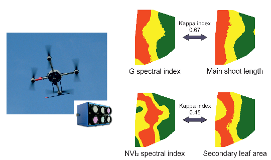
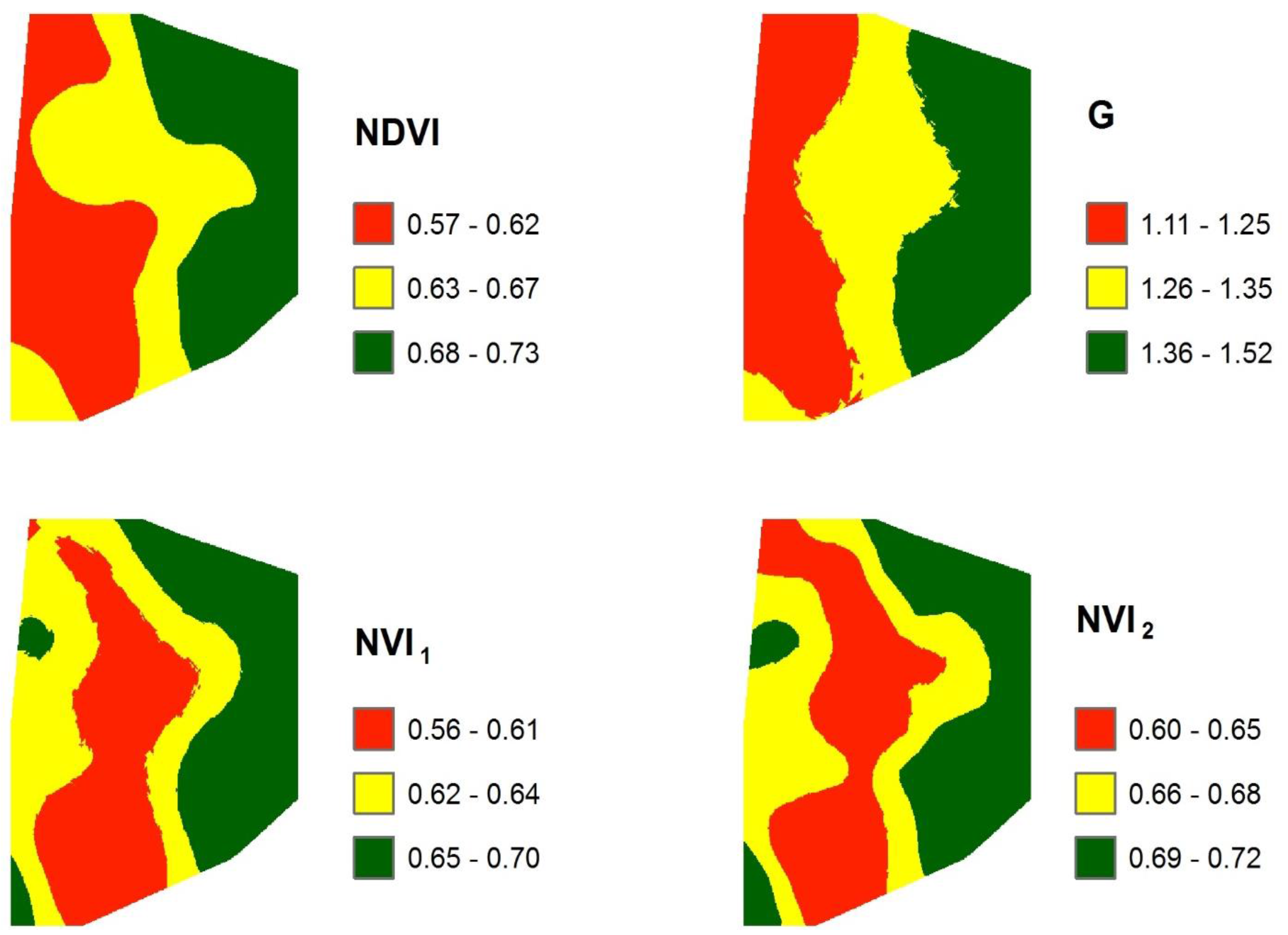
3.3. Mapping and Spatial Agreement between Spectral Indices and Field Variables

The mapping of the spectral indices has revealed the existence of spatial variability within the vineyard (Figure 3) regarding its vegetative and productive status. Classical indices such as NDVI or G exhibited maximum and minimum values at the East and West sides of the vineyard, respectively; while the two normalized indices, NVI1 and NVI2, placed the minimum values at the centre of the plot.
Figure 3. Maps obtained for spectral indices (NDVI, G, NVI1, and NVI2) in a Tempranillo (Vitis vinifera L.) vineyard. Maps were represented by terciles. AU: absorbance units.
Remotesensing 07 14458 g003
The spatial pattern of vegetative parameters (Figure 4), especially those related to main and secondary shoot length and leaf area matched that of NDVI and G. While the spatial behaviour of pruning weight better agreed with the spatial variability shown by the normalized indices NVI1 and NVI2 (Figure 3). Regarding the fluorescence-based indices related to leaf chlorophyll content and nitrogen status, they were also showing larger values on the East than on the West side of the vineyard (Figure 4).
Figure 4. Maps obtained for vegetative variables (pruning weight per vine, main shoot length, secondary shoot length, mail leaf area per shoot and secondary leaf area per shoot, leaf chlorophyll content (SFR_RAD) and nitrogen balance index (NBI_GAD)) in a Tempranillo (Vitis vinifera L.) vineyard. Maps were represented by terciles.
Remotesensing 07 14458 g004
Among yield parameters, only cluster weight exhibited a similar spatial pattern to that of vegetative variables and spectral indices (Figure 5). The clusters weighted more on the East side of the plot than in the centre and West sides of the plot, which corresponds, partially, with the spatial pattern of the new normalized indices, NVI1 and NVI2 (Figure 3), the pruning weight, and the nitrogen status of the vineyard (Figure 4). On the contrary, grapevines of the West part of the vineyard were found to be more productive in terms of yield per vine and number of clusters per vine, and less productive on the East side of the plot (Figure 5).
Figure 5. Maps obtained for yield parameters (cluster number per vine, cluster weight, yield per vine, and berry weight) in a Tempranillo (Vitis vinifera L.) vineyard. Maps were represented by terciles.
Remotesensing 07 14458 g005
High leaf area values do not always result in increased yield outputs as may occur in other crops such as cereals. In grapevines, yield is also related to the exposed leaf area (ELA), not only to total leaf area. As total leaf area increases, in Vertical Shoot Positioned systems, ELA reaches a point at which it cannot continue increasing, so the leaves that are not exposed may become a sink for the nutrients and energy of the plant competing with the clusters for these resources [61]. The lack of coincidence between areas of the vineyard, as the larger values of cluster number and yield per vine were in the East side of the plot while the larger values for the vigour spectral indices were in the West side (Figure 3 and Figure 5), might also be explained by the weather conditions in Spring 2010, as explained before.
Figure 6. Maps obtained for grape quality parameters (pH, total soluble solids, Titratable acidity, anthocyanins, and total phenols) in a Tempranillo (Vitis vinifera L.) vineyard. Maps were represented by terciles.
Remotesensing 07 14458 g006
Regarding berry composition, pH and TSS have shown the highest values on the East side of the plot and the lowest values on the West side (Figure 6). Consequently, titratable acidity showed the opposite behaviour, with higher values on the West side and lower on the East side, as the spectral index G (Figure 3). The anthocyanin concentration has showed a random pattern across the plot, while total phenols yielded the lowest values at the centre of the plot (Figure 6), increasing toward the sides, similar to the spatial pattern of NVI1 and NVI2 (Figure 3).
The visual match of the spatial patterns between the spectral indices and the in-field variables and berry composition was quantitatively assessed by carrying out a cross-tabulation and the computation of the kappa index from each variable 3-cluster-map. Table 4 shows the kappa index value for the cross-tabulation between the spectral indices and the in-field and berry composition variables. The kappa index yielded values ranging from –0.27 to 0.70, that is, from poor to substantial agreement, following the classification proposed by Landis and Koch [62].
Table 4. Cross-tabulation outputs and kappa index obtained for the classified maps of spectral indices (NDVI, G, NVI1, and NVI2), vegetative parameters (pruning weight, main shoot length, secondary shoot length, main leaf area per shoot, and secondary leaf area per shoot), fluorescence-based indices of nitrogen balance index (NBI_GAD) and chlorophyll content in leaves (SFR_RAD) for yield parameters (cluster number per vine, cluster weight, yield per vine, and berry weight) and for grape composition variables (pH, total soluble solids, titratable acidity, anthocyanins, and total phenols) in a Tempranillo (Vitis vinifera L.) vineyard.
NDVIGNVI1NVI2
Main shoot length0.410.670.180.17
Secondary shoot length0.470.590.450.44
Main leaf area0.430.700.190.16
Secondary leaf area0.470.570.460.45
Pruning weight0.320.080.390.35
SFR_R0.110.100.390.30
NBI_G0.320.360.380.35
Cluster number−0.26−0.27−0.17−0.15
Mean cluster weight0.350.350.370.40
Yield0.01−0.140.01−0.01
Mean berry weight0.120.110.130.12
pH0.140.35−0.05−0.05
Total soluble solids0.110.25−0.06−0.04
Titratable acidity−0.16−0.15−0.24−0.23
Anthocyanins−0.010.00−0.04−0.07
Total phenols0.00−0.02−0.09−0.08
These results show that, spatially speaking, the classical index G was the one showing a spatial pattern that best agreed with the spatial pattern of the vegetative variables, especially those regarding shoot length and leaf area, with values ranging from 0.59 for secondary shoot length (moderate agreement) to 0.70 for main leaf area (substantial agreement). Pruning weight, leaf chlorophyll content, and nitrogen status better concurred with the normalized index NVI1, yielding a fair agreement (~0.40). On the other hand, regarding the productive and berry composition variables, mean cluster weight and pH showed the highest kappa index values, especially with the normalized index NVI2 and G, respectively (0.40 and 0.35, fair agreement), while cluster number, yield, mean berry weight, pH, total soluble solids, titratable acidity, anthocyanins, and total phenols showed the lowest kappa coefficients with values indicating poor or slight agreement with the spectral indices, confirming the poor correlations observed.
The match of the spatial patterns is showing that, in general, the spectral indices derived from the multispectral images taken from a RPAS are useful tools for the grape-grower to manage the spatial variability of the vineyards. These indices seem to be more reliable for the management of the vegetative variables than for the productive and grape composition parameters, which is in agreement with the fact that the multispectral camera is retrieving the data from an overhead point of view, that is, from the canopy, not “seeing” the productive part of the grapevines located below the canopy. Therefore, while the multispectral sensor is directly sensing the vegetative component of the vineyard, the relation with the productive component of the vineyard remains indirect. Moreover, depending on the meteorological conditions in the season, more vigorous subareas of a vineyard plot may exhibit a higher water demand than less vigorous plants in a dry year, experiencing water stress that may jeopardize both grape yield and composition, while in cooler and less dry seasons, higher yield values are expected in vigorous plants.
In summary, the spectral indices obtained from the multispectral images captured from a RPAS have been shown to significantly correlate with the vegetative variables and some of the yield variables. Two newly defined spectral indices have also been provided that have shown the best correlations with important vegetative variables such as pruning weight, nitrogen status, or leaf chlorophyll content. The classical methods for the measurement of vegetative and yield parameters are laborious and generally destructive. Therefore, the spectral indices could be a useful tool to estimate these variables of interest in a fast and non-destructive way, at a time earlier than they could be assessed by the classical methods. Furthermore, multispectral images and their derived spectral indices provide the end-user with a continuous surface of data from the vineyard with high spatial resolution; that is, a large database that makes it possible to take into account the spatial variability of the vineyard status. This fact makes it operationally feasible to carry out a segmentation of the vineyard in 2 or 3 homogeneous management zones. In addition, compared to other remote sensing platforms, RPAS provide the grape-grower not only with higher spatial resolution, but also with higher flexibility to monitor their vineyards, especially the small vineyards prevailing in Europe (average vineyard size is less than 5 ha). Another important factor for the grape-grower that has not been profusely addressed in literature is the cost of applying remote sensing technologies. A very interesting paper has recently been published by Matese et al. [14] in which the authors carry out a cost comparison among three different remote sensing platforms: satellite, aircraft, and RPAS. Their results have shown that, for small surfaces (5 ha), as in the present work, the use of RPAS is the most cost-effective solution due to the lowest acquisition costs [14]. The situation changes with a higher surface of study (50 ha), as more images are needed to cover it, increasing the costs of acquisition, preprocessing, and analysis of these images. In this case, the satellite would be a more cost-effective choice, as it is able to cover a high surface with one image, decreasing the subsequent costs. To summarize, as shown by Matese et al. [14], each technology has technological, operational, and economic advantages and disadvantages and must be selected according to the work planned. In this study, some inconveniences regarding the operational factors of the flight were revealed. Despite greater independence and flexibility of RPAS systems, one of their disadvantages is that they are significantly affected by the wind, even by light wind, generating movements of the platform that were reflected in the images as geometric distortions. In addition, a lower flying height would result in a higher spatial resolution of the images, which should reduce the problem of the spectral mixture, providing pure vine pixels. These facts may lead to improved correlations between spectral indices and in-field variables.
Our results have shown that the three sub-zones delineated in the vineyard based on the spectral indices agreed with key vegetative parameters such as pruning weight, main leaf area, or main shoot length, and even with yield parameters such as mean cluster weight. It has been explored here by the application of kappa index, a common index usually used to assess land cover changes [63] that has proven very useful in assessing the agreement between the subareas delineated with spectral indices and the in-field variables. These variables have been proven to be temporally stable [49,64], so it could be useful to carry out vegetative management actions such as fertilisation, soil farming (i.e., inter-row cover cropping to limit the plant vigour in very vigorous subareas) and winter pruning in the following years. Furthermore, the possibility of customizing the filter selection for the multispectral camera may allow for collection of data in the shortwave infrared region of the spectrum if filters within this region are chosen, which could provide relevant information on the plant water status and could also provide interesting data regarding yield [65]. In this work, these new technologies made it possible to delineate three subzones of homogenous vegetative status within the vineyard, where the grape-grower could define its requirements and apply the appropriate inputs (water, nitrogen, etc.) or management practices for each subzone—that is, the implementation of precision viticulture techniques in the vineyard.

4. Conclusions

The results presented in this study confirm the potential of multi-sensor RPAS systems for the assessment of the spatial variability of the vineyard vegetative and productive status in precision viticulture. The two developed vegetation spectral indices, NVI1 and NVI2, were those best correlated with field vegetative parameters measured in sampling plots.
Moreover, the kappa index has shown that the spatial pattern of the spectral indices agreed with that of the vegetative and some of the productive variables measured in the vineyard. In this case, the classical spectral index G was the one showing the highest spatial agreement with the vegetative variables. The spectral indices enabled the delineation of three sub-zones of homogeneous management, within the frame of precision viticulture, to optimize the management of inputs (water, nitrogen, etc.), soil management, and winter pruning.
These results are a very important outcome because they proved that the use of a multispectral sensor mounted on a RPAS could become a reliable tool for the grape-growing industry to manage the spatial variability within the vineyard. The possibility of acquiring “on-demand” low-cost images with unprecedented high spatial resolution will certainly promote its operational application to vineyard management in order to improve crop productivity and sustainability.

Acknowledgments

This study was carried out as part of the Televitis project (Ref. ADER-2008-00187) funded by the Agencia de Desarrollo Tecnológico de La Rioja (La Rioja, Spain). Special gratitude goes to Airestudio Geoinformation Technologies S. Cop. for the acquisition of images with the RPAS. Additionally, we thank Javier Baluja and Victor Sicilia for collecting field data, and Inti Luna for his work on the image corrections.

Author Contributions

MPD and JT designed the study and implemented the experiments. CRC, MPM and AL analysed the data. CRC and MPD wrote the manuscript draft. All authors reviewed and approved the final manuscript.

Conflicts of Interest

The authors declare that this work was partially funded by Force-A by the lending of the sensors used.

References

  1. Tey, Y.S.; Brindal, M. Factors influencing the adoption of precision agricultural technologies: A review for policy implications. Precis. Agric. 2012, 13, 713–730. [Google Scholar] [CrossRef]
  2. Schieffer, J.; Dillon, C. The economic and environmental impacts of precision agriculture and interactions with agro-environmental policy. Precis. Agric. 2015, 16, 46–61. [Google Scholar] [CrossRef]
  3. Hall, A.; Lamb, D.W.; Holzapfel, B.; Louis, J. Optical remote sensing applications in viticulture-a review. Aust. J. Grape Wine Res. 2002, 8, 36–47. [Google Scholar] [CrossRef]
  4. Acevedo-Opazo, C.; Tisseyre, B.; Guillaume, S.; Ojeda, H. The potential of high spatial resolution information to define within-vineyard zones related to vine water status. Precis. Agric. 2008, 9, 285–302. [Google Scholar] [CrossRef]
  5. Baluja, J.; Diago, M.P.; Balda, P.; Zorer, R.; Meggio, F.; Morales, F.; Tardaguila, J. Assessment of vineyard water status variability by thermal and multispectral imagery using an unmanned aerial vehicle (UAV). Irrig. Sci. 2012, 30, 511–522. [Google Scholar] [CrossRef]
  6. Martin, P.; Zarco-Tejada, P.J.; Gonzalez, M.R.; Berjón, A. Using hyperspectral remote sensing to map grape quality in “tempranillo” vineyards affected by iron deficiency chlorosis. VITIS 2007, 46, 7–14. [Google Scholar]
  7. Zarco-Tejada, P.J.; Guillén-Climent, M.L.; Hernández-Clemente, R.; Catalina, A.; González, M.R.; Martín, P. Estimating leaf carotenoid content in vineyards using high resolution hyperspectral imagery acquired from an unmanned aerial vehicle (UAV). Agric. For. Meteorol. 2013, 171–172, 281–294. [Google Scholar] [CrossRef]
  8. Hall, A.; Louis, J.P.; Lamb, D.W. Low-resolution remotely sensed images of winegrape vineyards map spatial variability in planimetric canopy area instead of leaf area index. Aust. J. Grape Wine Res. 2008, 14, 9–17. [Google Scholar] [CrossRef]
  9. Mathews, A.; Jensen, J. Visualizing and quantifying vineyard canopy LAI using an unmanned aerial vehicle (UAV) collected high density structure from motion point cloud. Remote Sens. 2013, 5, 2164–2183. [Google Scholar] [CrossRef]
  10. Lamb, D.W.; Weedon, M.M.; Bramley, R.G.V. Using remote sensing to predict grape phenolics and colour at harvest in a cabernet sauvignon vineyard: Timing observations against vine phenology and optimising image resolution. Aust. J. Grape Wine Res. 2004, 10, 46–54. [Google Scholar] [CrossRef]
  11. Matese, A.; Capraro, F.; Primicerio, J.; Gualato, G.; Gennaro, S.F.D.; Agati, G. Mapping of vine vigor by UAV and anthocyanin content by a non-destructive fluorescence technique. In Precision Agriculture’13; Stafford, J., Ed.; Wageningen Academic Publishers: Wageningen, The Netherlands, 2013; pp. 201–208. [Google Scholar]
  12. Serrano Porta, L.; Zarco Tejada, P.; González Flor, C.; Pons Valls, J.M.; Gorchs Altarriba, G. Assessment of berry quality using airborne derived NDVI and PRI in rainfed vineyards. In Proceedings of the 9th European Conference on Precision Agriculture, Lleida, Spain, 7–11 July 2013.
  13. Turner, D; Lucieer, A.; Watson, C. Development of an unmanned aerial vehicle (UAV) for hyper resolution vineyard mapping based on visible, multispectral, and thermal imagery. In Proceedings of the 34th International Symposium on Remote Sensing of Environment, Sydney, NSW, Australia, 10–15 April 2011; p. 4.
  14. Matese, A.; Toscano, P.; Di Gennaro, S.; Genesio, L.; Vaccari, F.; Primicerio, J.; Belli, C.; Zaldei, A.; Bianconi, R.; Gioli, B. Intercomparison of uav, aircraft and satellite remote sensing platforms for precision viticulture. Remote Sens. 2015, 7, 2971–2990. [Google Scholar] [CrossRef]
  15. Berni, J.; Zarco-Tejada, P.J.; Suárez, L.; Fereres, E. Thermal and narrowband multispectral remote sensing for vegetation monitoring from an unmanned aerial vehicle. IEEE Trans. Geosci. Remote Sens. 2009, 47, 722–738. [Google Scholar] [CrossRef]
  16. Zhang, C.; Kovacs, J. The application of small unmanned aerial systems for precision agriculture: A review. Precis. Agric. 2012, 13, 693–712. [Google Scholar] [CrossRef]
  17. Jenkins, D.; Vasigh, B. The Economic Impact of Unmanned Aircraft Systems Integration in the United States. Available online: http://www.auvsi.org/econreport (accessed on 10 August 2015).
  18. Sepulcre-Cantó, G.; Diago, M.P.; Balda, P.; Martínez de Toda, F.; Morales, F.; Tardáguila, J. Monitoring vineyard spatial variability of vegetative growth and physiological status using an unmanned aerial vehicle (UAV). In Proceedings of the 16th International Symposium of GiESCO, Davis, CA, USA, 16–20 July 2009.
  19. Gamon, J.A.; Peņuelas, J.; Field, C.B. A narrow-waveband spectral index that tracks diurnal changes in photosynthetic efficiency. Remote Sens. Environ. 1992, 41, 35–44. [Google Scholar] [CrossRef]
  20. Martínez de Toda, F.; Tardáguila, J.; Sancha, J.C. Estimation of grape quality in vineyards using a new viticultural index. VITIS—J. Grapevine Res. 2007, 46, 168–173. [Google Scholar]
  21. Smart, R.; Robinson, M. Sunlight into Wine: A Handbook for Winegrape Canopy Management; Winetitles: Adelaida, SA, Australia, 1991. [Google Scholar]
  22. Ben Ghozlen, N.; Moise, N.; Latouche, G.; Martinon, V.; Mercier, L.; Besancon, E.; Cerovic, Z. Assessment of grapevine maturity using a new portable sensor: Non destructive quantification of anthocyanins. J. Int. Sci. Vigne Vin 2010, 44, 1–8. [Google Scholar]
  23. Ben Ghozlen, N.; Cerovic, Z.G.; Germain, C.; Toutain, S.; Latouche, G. Non-destructive optical monitoring of grape maturation by proximal sensing. Sensors 2010, 10, 10040–10068. [Google Scholar] [CrossRef] [PubMed]
  24. Tremblay, N.; Wang, Z.; Cerovic, Z. Sensing crop nitrogen status with fluorescence indicators. A review. Agron. Sustain. Dev. 2012, 32, 451–464. [Google Scholar] [CrossRef]
  25. Rey-Caramés, C. Assessment of the Spatial Variability of Vegetative Status in Vineyards Using Non-Destructive sensors. Application of Remote and Proximal Sensing Technologies in Precision Viticulture. Ph.D. Thesis, University of La Rioja, Logroño, Spain, 10 July 2015. [Google Scholar]
  26. OIV. Compendium of International Methods of Wine and Must Analysis; International Organisation of Vine and Wine: Paris, France, 2012. [Google Scholar]
  27. Iland, P.; Bruer, N.; Edwards, G.; Weeks, S.; Wilkes, E. Chemical Analysis of Grapes and Wine: Techniques and Concepts; Patrick Iland Wine Promotions: Campbelltown, SA, Australia, 2004. [Google Scholar]
  28. Sánchez-de-Miguel, P.; Baeza, P.; Junquera, P.; Lissarrague, J. Vegetative development: Total leaf area and surface area indexes. In Methodologies and Results in Grapevine Research; Delrot, S., Medrano, H., Or, E., Bavaresco, L., Grando, S., Eds.; Springer Netherlands: Dordrecht, The Netherlands, 2010; pp. 31–44. [Google Scholar]
  29. Laliberte, A.S.; Goforth, M.A.; Steele, C.M.; Rango, A. Multispectral remote sensing from unmanned aircraft: Image processing workflows and applications for rangeland environments. Remote Sens. 2011, 3, 2529–2551. [Google Scholar] [CrossRef]
  30. Inglada, J.; Christophe, E. The orfeo toolbox remote sensing image processing software. In Proceedings of the IEEE International Geoscience and Remote Sensing Symposium (IGARSS’09), Cape Town, South Africa, 12–17 July 2009; pp. 733–736.
  31. R Core Team. R: A Language and Environment for Statistical Computing; R Foundation for Statistical Computing: Vienna, Austria, 2012. [Google Scholar]
  32. Keitt, T.H.; Bivand, R.; Pebesma, E.; Rowlingson, B. Rgdal: Bindings for the Geospatial Data Abstraction Library. Available online: http://CRAN.R-project.org/package=rgdal (accessed on 10 August 2015).
  33. Hijmans, R.J.; van Etten, J. Raster: Geographic Analysis and Modeling with Raster Data. Available online: http://CRAN.R-project.org/package=raster (accessed on 10 August 2015).
  34. Rouse, J.W.; Haas, R.H.; Schell, J.A.; Deering, D.W.; Harlan, J.C. Monitoring the Vernal Advancements and Retrogradation of Natural Vegetation; NASA/GSFC Final Report; NASA: Greenbelt, MD, USA, 1974; pp. 1–371.
  35. Chen, J.M. Evaluation of vegetation indices and a modified simple ratio for boreal applications. Can. J. Remote Sens. 1996, 22, 229–242. [Google Scholar] [CrossRef]
  36. Haboudane, D.; Miller, J.R.; Pattey, E.; Zarco-Tejada, P.J.; Strachan, I.B. Hyperspectral vegetation indices and novel algorithms for predicting green LAI of crop canopies: Modeling and validation in the context of precision agriculture. Remote Sens. Environ. 2004, 90, 337–352. [Google Scholar] [CrossRef]
  37. Roujean, J.L.; Breon, F.M. Estimating par absorbed by vegetation from bidirectional reflectance measurements. Remote Sens. Environ. 1995, 51, 375–384. [Google Scholar] [CrossRef]
  38. Qi, J.; Chehbouni, A.; Huete, A.; Kerr, Y.; Sorooshian, S. A modified soil adjusted vegetation index. Remote Sens. Environ. 1994, 48, 119–126. [Google Scholar] [CrossRef]
  39. Rondeaux, G.; Steven, M.; Baret, F. Optimization of soil-adjusted vegetation indices. Remote Sens. Environ. 1996, 55, 95–107. [Google Scholar] [CrossRef]
  40. Daughtry, C.S.T.; Walthall, C.L.; Kim, M.S.; De Colstoun, E.B.; McMurtrey, J.E. Estimating corn leaf chlorophyll concentration from leaf and canopy reflectance. Remote Sens. Environ. 2000, 74, 229–239. [Google Scholar] [CrossRef]
  41. Haboudane, D.; Miller, J.R.; Tremblay, N.; Zarco-Tejada, P.J.; Dextraze, L. Integrated narrow-band vegetation indices for prediction of crop chlorophyll content for application to precision agriculture. Remote Sens. Environ. 2002, 81, 416–426. [Google Scholar] [CrossRef]
  42. Jordan, C.F. Derivation of leaf-area index from quality of light on the forest floor. Ecology 1969, 50, 663–666. [Google Scholar] [CrossRef]
  43. Bramley, R.G.V. Understanding variability in winegrape production systems 2. Within vineyard variation in quality over several vintages. Aust. J. Grape Wine Res. 2005, 11, 33–42. [Google Scholar] [CrossRef]
  44. Pebesma, E.J. Multivariable geostatistics in S: The gstat package. Comput. Geosci. 2004, 30, 683–691. [Google Scholar] [CrossRef]
  45. Hudson, W.D.; Ramm, C.V. Correct formulation of the kappa coefficient of agreement. Photogramm. Eng. Remote Sens. 1987, 53, 421–422. [Google Scholar]
  46. Gitelson, A.A.; Kaufman, Y.J.; Merzlyak, M.N. Use of a green channel in remote sensing of global vegetation from EOS-MODIS. Remote Sens. Environ. 1996, 58, 289–298. [Google Scholar] [CrossRef]
  47. Baluja, J.; Diago, M.P.; Goovaerts, P.; Tardaguila, J. Assessment of the spatial variability of anthocyanins in grapes using a fluorescence sensor: Relationships with vine vigour and yield. Precis. Agric. 2012, 13, 457–472. [Google Scholar] [CrossRef]
  48. Bramley, R.; Lamb, D. Making sense of vineyard variability in Australia. In Proceedings of the International Symposium on Precision Viticulture, Ninth Latin American Congress on Viticulture and Oenology, Santiago, Chile, 24–28 November 2003; pp. 35–54.
  49. Bramley, R.G.V.; Hamilton, R.P. Understanding variability in winegrape production systems 1. Within vineyard variation in yield over several vintages. Aust. J. Grape Wine Res. 2004, 10, 32–45. [Google Scholar] [CrossRef]
  50. Agati, G.; Foschi, L.; Grossi, N.; Guglielminetti, L.; Cerovic, Z.G.; Volterrani, M. Fluorescence-based versus reflectance proximal sensing of nitrogen content in Paspalum vaginatum and Zoysia matrella turfgrasses. Eur. J. Agron. 2013, 45, 39–51. [Google Scholar] [CrossRef]
  51. Cartelat, A.; Cerovic, Z.G.; Goulas, Y.; Meyer, S.; Lelarge, C.; Prioul, J.L.; Barbottin, A.; Jeuffroy, M.H.; Gate, P.; Agati, G.; et al. Optically assessed contents of leaf polyphenolics and chlorophyll as indicators of nitrogen deficiency in wheat (Triticum aestivum L.). Field Crops Res. 2005, 91, 35–49. [Google Scholar] [CrossRef]
  52. Cerovic, Z.G.; Goutouly, J.-P.; Hilbert, G.; Destrac-Irvine, A.; Martinon, V.; Moise, N. Mapping winegrape quality attributes using portable fluorescence-based sensors. Frutic 2009, 9, 301–310. [Google Scholar]
  53. Oliver, M.A. Geostatistical Applications for Precision Agriculture; Springer: London, UK, 2010. [Google Scholar]
  54. Taylor, J.A.; Bates, T.R. Sampling and estimating average pruning weights in concord grapes. Am. J. Enol. Vitic. 2012, 63, 559–563. [Google Scholar] [CrossRef]
  55. Cambardella, C.A.; Moorman, T.B.; Parkin, T.B.; Karlen, D.L.; Novak, J.M.; Turco, R.F.; Konopka, A.E. Field-scale variability of soil properties in central Iowa soils. Soil Sci. Soc. Am. J. 1994, 58, 1501–1511. [Google Scholar] [CrossRef]
  56. Bonilla, I.; Martinez de Toda, F.; Martínez-Casasnovas, J.A. Vine vigor, yield and grape quality assessment by airborne remote sensing over three years: Analysis of unexpected relationships in cv. Tempranillo. Span. J. Agric. Res. 2015, 13, 1–8. [Google Scholar] [CrossRef]
  57. Dobrowski, S.Z.; Ustin, S.L.; Wolpert, J.A. Grapevine dormant pruning weight prediction using remotely sensed data. Aust. J. Grape Wine Res. 2003, 9, 177–182. [Google Scholar] [CrossRef]
  58. Hall, A.; Lamb, D.W.; Holzapfel, B.P.; Louis, J.P. Within-season temporal variation in correlations between vineyard canopy and winegrape composition and yield. Precis. Agric. 2011, 12, 103–117. [Google Scholar] [CrossRef]
  59. Proffitt, T.; Malcolm, A. Implementing zonal vineyard management through airborne remote sensing. Aust. N. Z. Grapegrow. Winemak. 2005, 502, 22–27. [Google Scholar]
  60. Keller, M.; Tarara, J.M.; Mills, L.J. Spring temperatures alter reproductive development in grapevines. Aust. J. Grape Wine Res. 2010, 16, 445–454. [Google Scholar] [CrossRef]
  61. Martínez de Toda, F. Claves de la Viticultura de Calidad, Nuevas Técnicas de Estimación y Control de la Calidad de la Uva en el Viñedo. Mundi-Prensa: Madrid, Spain, 2011. [Google Scholar]
  62. Landis, J.R.; Koch, G.G. The measurement of observer agreement for categorical data. Biometrics 1977, 33, 159–174. [Google Scholar] [CrossRef] [PubMed]
  63. Congalton, R.G.; Green, K. Assessing the Accuracy of Remotely Sensed Data; CRC Press: Boca Raton, FL, USA, 2008. [Google Scholar]
  64. Tisseyre, B.; Mazzoni, C.; Fonta, H. Whithin-field temporal stability of some parameters in viticulture: Potential toward a site specific management. J. Int. Sci. Vigne Vin. 2008, 42, 27. [Google Scholar]
  65. Serrano, L.; González-Flor, C.; Gorchs, G. Assessment of grape yield and composition using the reflectance based water index in Mediterranean rainfed vineyards. Remote Sens. Environ. 2012, 118, 249–258. [Google Scholar] [CrossRef] [Green Version]

