Assessing the Potential to Operationalize Shoreline Sensitivity Mapping: Classifying Multiple Wide Fine Quadrature Polarized RADARSAT-2 and Landsat 5 Scenes with a Single Random Forest Model

Abstract

The Random Forest algorithm was used to classify 86 Wide Fine Quadrature Polarized RADARSAT-2 scenes, five Landsat 5 scenes, and a Digital Elevation Model covering an area approximately 81,000 km² in size, and representing the entirety of Dease Strait, Coronation Gulf and Bathurst Inlet, Nunavut. The focus of this research was to assess the potential to operationalize shoreline sensitivity mapping to inform oil spill response and contingency planning. The impact of varying the training sample size and reducing model data load were evaluated. Results showed that acceptable accuracies could be achieved with relatively few training samples, but that higher accuracies and greater probabilities of correct class assignment were observed with larger sample sizes. Additionally, the number of inputs to the model could be greatly reduced without impacting overall performance. Optimized models reached independent accuracies of 91% for seven land cover types, and classification probabilities between 0.77 and 0.98 (values for latter represent per-class averages generated from independent validation sites). Mixed results were observed when assessing the potential for remote predictive mapping by simulating transferability of the model to scenes without training data.

1. Introduction

Arctic marine shorelines are sensitive environments that can experience both immediate and long-term perturbations from oil spills, which may occur more frequently as a result of increased energy resource development and transportation in the Canadian Arctic [1,2,3,4,5,6]. In the event of a marine oil spill, detailed maps of the affected area are required to inform response operations as protection strategies and cleaning techniques differ depending on the shoreline type present. Both the predominant substrate type (e.g., sand vs. pebbles) and physical form (e.g., beach vs. flat) must be indicated as this largely determines the extent to which surface permeability and exposure permit oil to persist within the natural environment, as well as the appropriate treatment strategy [7,8]. Information on the extent and location of sensitive cultural and biological resources is also required to facilitate the use of spill countermeasures, including containment booms, which can prevent further spreading. In Canada, these so-called “shoreline sensitivity maps” have been prepared for the Great Lakes and majority of shorelines along the east and west coasts, however, relatively few areas throughout the Arctic have ever been systematically surveyed. Many of the maps that do exist are also decades old and based on outdated technology. As changing climatic conditions, including longer open water seasons, are expected to promote increased ship traffic and natural resource development, it is vital that response contingency plans are established for these areas.

For over 30 years helicopter videography has been the primary data source for generating shoreline sensitivity maps in Canada. Typically analysts fly parallel along the coast, recording videos and audio commentaries in which they describe the predominant substrate type and physical form of the lower, middle, and upper intertidal zones (land exposed at low tide and covered by water at high tide), the supratidal zone (affected only by wave action and spray), and the backshore (not affected by marine processes, but used for access and staging purposes) [9]. This information is then transferred to a Geographic Information System through the manual segmentation of a vector file (representing the land-water interface) into homogeneous units [8]. In the event of a spill this information can then be used to make real-time decisions regarding the allocation of resources and personnel; improving response efficiency, and reducing long-term impacts on the environment [10].

There are, however, additional logistical problems and higher costs associated with implementing this approach in vast, remote areas such as the Canadian Arctic. For example, there are relatively few sites for helicopters to refuel necessitating the use of fuel caches, especially on extended flights. This increases costs as additional flights are required to first deposit the fuel, then to collect the empty containers. In light of this, there is interest in developing a semi-automated mapping approach using Earth observation data [11,12,13]. Accordingly, the purpose of this study was to assess the potential to operationalize shoreline sensitivity mapping over a large region, using a single model to classify data that have been demonstrated to provide relevant and complementary information for this application [11,12,13]; specifically, multiple RADARSAT-2 Synthetic Aperture Radar (SAR), and Landsat 5 optical scenes (images necessarily acquired on different dates and with different spatial footprints to provide full study site coverage), as well as a Digital Elevation Model (DEM). For this we used the Random Forest algorithm; a non-parametric classifier based on an ensemble of individual decision tree models [14]. Products from this analysis will be used to support oil spill response and contingency planning throughout the region.

2. Background

2.1. Potential for Shoreline Sensitivity Mapping Using Earth Observation Data: A Review of Relevant Literature

Few studies have focused on assessing the potential for shoreline sensitivity mapping using Earth observation data, though of the studies that do exist, a number were undertaken in the Canadian Arctic [11,12,13]. Potential for this application has also been demonstrated in other regions [15,16]. Additional, relevant research has shown that it is possible to map more general Arctic land cover types [17].

Banks et al. [11] assessed the potential to classify shore and near-shore land cover types over two study areas: Richards Island and Tuktoyaktuk Harbour, Northwest Territories, Canada. The authors acquired three Fine Quadrature Polarized (Quad Pol) RADARSAT-2 scenes over each site to assess the impact of incidence angle on class separability, and classification accuracy. Analysis of the Bhattacharyya Distance and of relevant statistics indicated that steep angles (~21°–24°) were generally preferred for discriminating wetlands from other land covers (e.g., tall shrubs), while shallow angles (~45°–50°) were generally preferred for discriminating classes of varying surface roughnesses (e.g., sand beaches/flats from mixed sediment beaches/flats). Shallow incidence angle images also provided the best overall class separability, and when the three intensity channels (HH, HV and VV in dB) were combined with SPOT-4 imagery as inputs to the Maximum Likelihood classifier, the authors achieved overall accuracies of 76% and 86% for the Richards Island and Tuktoyaktuk Harbour sites, respectively. While it was not known what the weather conditions were immediately prior to each acquisition, potential for classifier transferability was demonstrated as the authors showed that values for many classes were consistent between the two study areas when compared at like incidence angles.

In a follow-up paper Banks et al. [12] assessed the potential to classify shore and near-shore land cover types using unsupervised polarimetric SAR classifiers, including: Wishart-entropy/alpha, Wishart-entropy/anisotropy/alpha, and Freeman-Wishart [18,19]. The authors applied each classifier to the same six images used by Banks et al. [11], and found that they could detect more land covers using the shallow and medium incidence angle images. In general though, classification results obtained by combining available SAR and optical data in the Maximum Likelihood classifier by Banks et al. [11], were superior to results obtained with the polarimetric SAR classifiers. The authors also applied the Cloude-Pottier and Freeman-Durden decompositions [20,21,22] to characterize scattering behaviour, and assess the consistency of values between sites at like incidence angles. While in most cases outputs from the Cloude-Pottier decomposition were similar, Freeman-Durden decomposition variables, especially the double bounce parameter, showed high variability.

Demers et al. [13] compared pixel-based Maximum Likelihood and hierarchical object-based classifiers over two study areas: Richards Island, Northwest Territories, Canada and Ivvavik, Yukon, Canada. By combining the intensity channels and Freeman-Durden decomposition parameters from Fine Quad Pol RADARSAT-2 imagery, the spectral channels and Normalized Difference Vegetation Index (NDVI) data from SPOT-4 imagery, as well as a DEM, the authors achieved overall accuracies of 73% for both sites with the pixel-based approach, and overall accuracies of 74% and 63% at Richards Island, and Ivvavik with the hierarchical object-based approach. The authors demonstrated potential for classifier transferability by applying both models trained on data from the Richards Island site to the Ivvavik site, achieving overall accuracies of 71% and 78% for the pixel and object-based approaches, respectively. Notably, these results were attained with RADARSAT-2 images that were acquired on different dates, and at different incidence angles (~34°–36° (FQ15) over Richards Island, and ~48°–49° (FQ30) over Ivvavik), the latter of which has been shown to affect the backscattering behaviour of some shoreline classes [11,12].

Potential has also been demonstrated for manual shoreline mapping through visual interpretation of fused optical and SAR data. Souza-Filho et al. [15] used a Red Green Blue/Intensity Hue Saturation transformation to integrate Landsat and Fine RADARSAT-1 data in order to identify geobotanical features along the Amazonian mangrove coast of Brazil. The authors were able to visually discriminate 19 land cover types, including: sand flats, mudflats, barrier beach ridges, sand ridges, marshes, and various mangrove stands, and with the aid of field data, were able to create a geomorphological map of the area. Souza-Filho et al. [16] used a similar approach to manually generate a shoreline sensitivity map of their study area, which was also located along the coast of Brazil. Their research showed potential to identify 10 unique land cover types, which were differentiated on the basis of their sensitivity to oiling.

Ullmann et al. [17] assessed the potential to classify five land cover types along the outer Mackenzie Delta, Northwest Territories, Canada, including: water, bare substrate, low/grass and herb dominated tundra, medium/herb dominated tundra, high/shrub dominated tundra, and wetlands. The authors compared results for supervised and unsupervised classification methods using different combinations of Dual Pol TerraSAR-X, Quad Pol RADARSAT-2, and Landsat 8 imagery. The optimal combination and method included both RADARSAT-2 and Landsat 8 data in a supervised classifier, which achieved an overall accuracy of 87%. The authors also observed potential for unsupervised classification of wetlands and non-vegetated substrates, due to the former showing dominant double bounce scattering, while the latter showed dominant surface scattering.

To some extent these studies have all demonstrated the complementarity of SAR and optical data for mapping shore and near-shore land cover types. Both Banks et al. [11,12] attempted to classify SAR imagery alone, but found lower accuracies compared to those achieved with SAR and optical data [11]. Banks et al. [11] also found that both data types were required to discriminate sand from mixed-sediment beaches and flats. With their hierarchical object-based classifier, Demers et al. [13] observed that some classes were better detected with either SAR or optical data (e.g., vegetated and un-vegetated features were better differentiated with NDVI values; Freeman-Durden double bounce and HH/HV values were better for detecting wetlands). Souza-Filho et al. [15,16] found that fusing optical and SAR imagery together improved their ability to visually discriminate features, and Ullmann et al. [17] also found that the combination of SAR and optical imagery produced higher classification accuracies. Based on these results we chose to use both SAR and optical imagery in this research.

2.2. The Random Forest Classifier

The Random Forest algorithm is a non-parametric classifier that uses bagging and a voting procedure to predict the majority output from an ensemble of individual decision tree classifiers [14]. It has proven effective for classifying highly dimensional data (i.e., many input variables) from a variety of sensors [23,24,25,26], and has been shown to outperform conventional parametric classifiers, including Maximum Likelihood [23,27,28,29]. This is particularly relevant with respect to the classification of SAR data, since backscatter values are not typically normally distributed when represented in linear power format [11]. As such, some authors maintain that non-parametric approaches like Random Forest are better suited to classifying these, as well as other multi-source datasets [27,30,31,32,33].

A number of authors have also achieved comparable or improved results with Random Forest, compared to other non-parametric approaches, including Classification and Regression Trees (CARTs) [23,27,30,34], Support Vector Machines [29,35,36,37], and Neural Networks [29]. These approaches typically require more user-interference with classifier settings whereas Random Forest only requires that users define: (1) the number of trees that are generated; and (2) the number of variables tested during each iteration of node splitting (described subsequently); a benefit that is commonly noted in the literature [24,38,39]. Additionally, there is no need to spend time analyzing or pruning individual trees as is the case for single CART models.

Some authors have also demonstrated that Random Forest performs well, even with a relatively small training sample size. Waske and Braun [27] classified multi-temporal SAR imagery and evaluated the effect of changes to training sample size on classifier performance. The authors observed that accuracy was not overly dependent on training sample size, and that acceptable accuracies could be achieved with as few as 50 sample sites per-class. Ham et al. [40] classified two study sites using hyperspectral data with limited training data, and observed only marginal improvements when their training sample size was increased from 15% to 75% of their total datasets (each of which contained 5211 and 3245 training samples in total, for each of the two study areas). The effect of training sample size on classifier performance is an important consideration for Arctic shoreline mapping applications, since these areas tend make up a relatively small proportion of the total image, leading to fewer available training sites [11,12,13]. In addition, these areas tend to be remote, which makes them difficult and expensive to access for extended periods.

The supervised Random Forest classification approach works by generating a user-defined number (ensemble or “forest”) of CART-like classifiers that are built from, and subsequently tested, using a random bootstrapped sample of a training/internal validation dataset provided by the user [30]. Sampling with replacement generates different subsets for each tree, with the proportion of each remaining constant at about two thirds for training and one third for internal validation. To determine the split at each node, a random subset of available predictor variables are tested, and only that variable which provides the best split is used [38,41]. This approach seeks to reduce the degree of correlation amongst individual trees in the forest, which often improves performance and enables the use of both independent and dependent data [14,27,30,31,34]. The model is also said to be robust to overfitting, and since only a subset of all variables are used to determine the split at each node, the algorithm is more computationally efficient than other methods (e.g., boosting), which better permits the use of highly dimensional datasets [27,30,31].

Once the forest is built image values at each pixel are run down all trees. However, because each tree is built from different training data, input variables, and split rules, the final output (per-pixel class prediction) may differ among each tree in the forest [26]. As such, a voting procedure is utilized, whereby each fully-grown tree casts a single vote and the majority is provided as the final output. In doing so errors that could be produced by the individual classifiers are potentially avoided as it assumed that the same errors are not generated by the majority [27,39,42,43]. A cumulative error estimate called the Out of Bag Error (OOBE) is also produced, which is based on the results achieved during the internal validation process applied to each tree. Under certain conditions it may be possible to use this in place of an independent accuracy assessment as the OOBE values can be comparable to independent error estimates [14].

The Random Forest algorithm also produces measures of variable importance, which can be used to determine which inputs contribute predictive ability within the overall model. Not only does this provide insight into the underlying structure within the multivariate dataset, it can also be used to perform variable reduction to increase computational efficiency. Specifically, the script used in this analysis reads in values for each image channel at all training sites. Depending on the number of inputs, this process can be time consuming [25,26]. It has also been demonstrated that using just the most important variables can significantly improve overall accuracy [25].

Within the “randomForest” package currently available in R (used in the present analysis), it is possible to generate two measures of importance: that which is based on the Gini index, and that which is based on the Mean Decrease in Accuracy [38]. Values for the former provide an indication of the extent to which the variable generates homogeneous or pure nodes, while the latter is based on a relative change in accuracy as a result of the variable being randomly permuted or excluded from the model. In both cases, higher values indicate higher importance [14,38,44]. Importance values can also vary greatly among models built on the same predictor variables, although it has been shown that values become more stable when a high number of trees are built into the forest [38].

3. Objectives

The overarching objective of this research was to assess the potential to operationalize shoreline sensitivity mapping through the use of a single Random Forest model to classify multiple RADARSAT-2 and Landsat 5 scenes acquired over a large, remote area. Our specific objectives were to:

• Assess the effect of training sample size on classifier accuracies and probabilities. Obtaining a large amount of training data for remote Arctic shorelines can be challenging since these areas are both expensive and difficult to access. It can also be difficult to generate a sufficient number of training sites because many shoreline features tend to make up a relatively small proportion of the total image area [11,12,13]. To help plan future shoreline mapping work along other Arctic coasts, we determined the smallest training sample size required to classify each of the land cover types considered to an acceptable level.
• Determine which predictor variables provide relevant information to the model and assess the effect of reducing the data load on classifier accuracies and probabilities. Preparing images for classification is time consuming, especially if multiple variables need to be generated for multiple scenes, and for multiple image types. Storing and classifying these highly dimensional datasets can also be computationally expensive. To decrease image processing times and storage requirements, as well as to increase computational efficiency of the model, we assessed the extent to which variables with relatively low importance values could be removed from the model, while still maintaining or improving classifier accuracies and probabilities.
• Assess the potential for remote predictive mapping. To map areas that are expensive or difficult to access, it would be advantageous to generate shoreline maps without collecting new field data. As such, we assessed the potential for remote predictive mapping by excluding training data from one in five helicopter videography surveys (collected in lieu of conventional ground data; described subsequently) to simulate application of model to areas without any training data.

4. Materials and Methods

4.1. Study Area

The study area considered in this research is located between Dolphin and Union Strait, and Queen Maud Gulf, encompassing the entirety of Coronation Gulf, Dease Strait, and Bathurst Inlet in the Kitikmeot region of Nunavut (Figure 1). Together these waterways divide Victoria Island from the mainland, representing a potential route along the Northwest Passage. There are two main communities within the region: Kugluktuk (formerly Coppermine) which is situated at the mouth of the Coppermine River to the west, and Cambridge Bay on the southeastern side of Victoria Island. Houses, fishing, and hunting camps are also found intermittently along the coast. The last shoreline sensitivity map generated for the area was commissioned by Environment Canada over twenty years ago [45].

Areas south of Rae River along the mainland fall on the northernmost extent of Canadian Shield, while the sedimentary rocks forming the Arctic Platform are found in the lowlands to north and on Victoria Island (Figure 1). Glacial and marine deposits cover most of the landscape, while the underlying bedrock is visible in some areas along the coast and on several islands offshore. Coastal features consist primarily of low lying beaches with varying proportions of gravel and sand, beach ridges/berms, raised beach ridges, bedrock platforms, cliffs, and talus slopes, deltas and bars at the mouths of rivers, and low lying tundra, and wetlands [45,46].

4.2. Land Cover Classes

The land cover classes considered in this analysis are presented in Table 1. These have been adapted from the 25 land cover types currently used by Environment Canada for shoreline sensitivity mapping [8]. By combining expert knowledge from previous studies [11,12,13] with preliminary classifier results, and class-specific descriptive statistics (e.g., mean, mode, standard deviation, and range), some land covers with similar morphologies, sediments, and or vegetation types were merged to form more general classes (Table 1). For example, the decision was made not to differentiate between tidal flats and beaches, since analysts often confuse these features in manual shoreline mapping/segmentation [8]. Similarly, sandy materials tend to be misidentified as mud and vice versa [8]. All areas visible in the intertidal, supratidal, and backshore zones were also classified together, and no attempt was made to differentiate them from one another [13].

Figure 1. Map of Canada (left) and of the study area considered in this research (right) showing coverage of the RADARSAT-2 and Landsat 5 data (represented as same-day strips), as well as the portions of the coast along which helicopter videography surveys were completed. The estimated length of shoreline covered is indicated on each line segment.

Figure 1. Map of Canada (left) and of the study area considered in this research (right) showing coverage of the RADARSAT-2 and Landsat 5 data (represented as same-day strips), as well as the portions of the coast along which helicopter videography surveys were completed. The estimated length of shoreline covered is indicated on each line segment.

Table 1. Shoreline types used by Environment Canada in conventional shoreline sensitivity mapping, and the generalized land cover classes considered in this analysis. Note that a general tundra class is not defined in conventional shoreline sensitivity mapping.

Adapted Land Cover Class for This Analysis	Shoreline Type	Description 1	Sensitivity Information 2
Water	Water	All open water including rivers, lakes, ponds and the ocean.	N/A
Mud/Sand	Mud Tidal Flat	Dominant grain size: 0.00024 to 0.0625 mm; slope < 5°; other sediments present but cover < 10% of surface.	Important species habitat, particularly for migrant birds and burrowing animals.
	Sand Beach	Dominant grain size: 0.0625 to 2 mm; slope > 5°; other sediments present but cover < 10% of surface.	With the exception of some low energy environments, biological productivity is generally low due to frequent reworking of the surface.
	Sand Tidal Flat	Dominant grain size: 0.0625 to 2 mm; slope < 5°; other sediments present but cover < 10% of surface.	Typically contain larvae, worms and insects that migratory bird species feed on during the summer months.
Mixed Sediment	Mixed Sediment Beach	Primarily fine grained sediments (sand and mud), with coarser materials (pebbles, cobbles, boulders) making up some proportion that is > 10% of the surface. Slope is > 5°.	In sheltered areas plants and animals are able to survive, however in areas that are regularly reworked, biological productivity is often low.
	Mixed Sediment Tidal Flat	Primarily fine grained sediments (sand and mud), with coarser materials (pebbles, cobbles, boulders) making up some proportion that is > 10% of the surface. Slope is < 5°.	In sheltered areas plants and animals are able to survive, however in areas that are regularly reworked, biological productivity is often low.
Pebble/Cobble/Boulder	Pebble/Cobble Beach	Dominant grain size: 4 to 256 mm; other sediments present but cover < 10% of surface.	Low biological productivity in general, due to constant reworking of materials.
	Boulder Beach	Dominant grain size: > 256 mm; other sediments present but cover < 10% of surface.	Biological productivity may be high, since these shorelines are stable.
Bedrock	Bedrock	Bedrock outcrop, plateau or ramp. Other sediments present but cover < 10% of surface.	Biological productivity is relatively low.
Wetland	Marsh	Wetlands containing saline-adapted plant species, including sedges, grasses, rushes, and reeds [48].	Important species habitat; highly productive environments.
	Wetland	According to Owens [47], marshes and wetlands are differentiated on the basis of species composition. Wetlands are predominated by grasses, which are salt tolerant.	Important species habitat; highly productive environments.
Tundra	NA	All non-marsh and non-wetland areas that are vegetated.	N/A

¹ Unless otherwise indicated information in this column has been summarized from Owens [47]. ² Unless otherwise indicated information in this column has been summarized from Owens et al. [48].

Table 1. Shoreline types used by Environment Canada in conventional shoreline sensitivity mapping, and the generalized land cover classes considered in this analysis. Note that a general tundra class is not defined in conventional shoreline sensitivity mapping.

Adapted Land Cover Class for This Analysis	Shoreline Type	Description 1	Sensitivity Information 2
Water	Water	All open water including rivers, lakes, ponds and the ocean.	N/A
Mud/Sand	Mud Tidal Flat	Dominant grain size: 0.00024 to 0.0625 mm; slope < 5°; other sediments present but cover < 10% of surface.	Important species habitat, particularly for migrant birds and burrowing animals.
	Sand Beach	Dominant grain size: 0.0625 to 2 mm; slope > 5°; other sediments present but cover < 10% of surface.	With the exception of some low energy environments, biological productivity is generally low due to frequent reworking of the surface.
	Sand Tidal Flat	Dominant grain size: 0.0625 to 2 mm; slope < 5°; other sediments present but cover < 10% of surface.	Typically contain larvae, worms and insects that migratory bird species feed on during the summer months.
Mixed Sediment	Mixed Sediment Beach	Primarily fine grained sediments (sand and mud), with coarser materials (pebbles, cobbles, boulders) making up some proportion that is > 10% of the surface. Slope is > 5°.	In sheltered areas plants and animals are able to survive, however in areas that are regularly reworked, biological productivity is often low.
	Mixed Sediment Tidal Flat	Primarily fine grained sediments (sand and mud), with coarser materials (pebbles, cobbles, boulders) making up some proportion that is > 10% of the surface. Slope is < 5°.	In sheltered areas plants and animals are able to survive, however in areas that are regularly reworked, biological productivity is often low.
Pebble/Cobble/Boulder	Pebble/Cobble Beach	Dominant grain size: 4 to 256 mm; other sediments present but cover < 10% of surface.	Low biological productivity in general, due to constant reworking of materials.
	Boulder Beach	Dominant grain size: > 256 mm; other sediments present but cover < 10% of surface.	Biological productivity may be high, since these shorelines are stable.
Bedrock	Bedrock	Bedrock outcrop, plateau or ramp. Other sediments present but cover < 10% of surface.	Biological productivity is relatively low.
Wetland	Marsh	Wetlands containing saline-adapted plant species, including sedges, grasses, rushes, and reeds [48].	Important species habitat; highly productive environments.
	Wetland	According to Owens [47], marshes and wetlands are differentiated on the basis of species composition. Wetlands are predominated by grasses, which are salt tolerant.	Important species habitat; highly productive environments.
Tundra	NA	All non-marsh and non-wetland areas that are vegetated.	N/A

¹ Unless otherwise indicated information in this column has been summarized from Owens [47]. ² Unless otherwise indicated information in this column has been summarized from Owens et al. [48].

4.3. RADARSAT-2 Acquisitions and Available Landsat 5 Data

Two passes of Single Look Complex Wide Fine Quad Pol RADARSAT-2 data with a nominal pixel spacing of 8.2 m and a 35° incidence angle at NADIR (FWQ21 beam mode) were acquired over the majority of the study area between August and September of 2014 (Table 2). The shallowest of available incidence angles was selected since: (1) these data are provided at a higher spatial resolution, so could combined with higher resolution optical data if it were made available; (2) the effects of foreshortening are reduced (albeit with increased image shadow) [49]; and (3) previous studies have indicated that shallow angles are generally preferred for this application [11,12]. All images were acquired using the same beam mode, since backscatter values for some specific shore and near-shore land cover types can show incidence angle dependence [11,12]. Each scene was acquired with the Land Look-up Table, in the ascending look direction, and was provided with Definitive Orbit information.

Of the two available passes, those images that appeared to have calmer sea states (less wave activity) and were believed to be acquired under relatively dry weather conditions were used in this analysis. Unfortunately weather information could only be obtained from stations at Kugluktuk and Cambridge Bay, which are hundreds of kilometres away from some scenes. As such, visual comparisons were also used to assess scene-to-scene consistency. In all cases but one, this resulted in the selection of the August acquisition (Table 2). While not a focus here, future work will assess the effect of combining both passes on classifier accuracy.

Table 2. Wide Fine Quad Pol RADARSAT-2 data acquired for this research. All training and validation sites fell on those images that are greyed out. Two complete passes were acquired for each image strip with exception of strip 8 (only first pass acquired), and strips 9 and 10 (second pass only covered a portion of the first same-day strip).

Image Strip (West to East)	Acquisition Timing	Number of Scenes Per-Pass
1	26 August 2014	4
2	9 August 2014	5
3	16 August 2014	6
4	23 August 2014	6
5	6 August 2014	6
6	13 August 2014	9
7	20 August 2014	14
8	3 August 2014	12
9	10 August 2014	7
10	10 August 2014	8
11	24 August 2014	9

Table 2. Wide Fine Quad Pol RADARSAT-2 data acquired for this research. All training and validation sites fell on those images that are greyed out. Two complete passes were acquired for each image strip with exception of strip 8 (only first pass acquired), and strips 9 and 10 (second pass only covered a portion of the first same-day strip).

Image Strip (West to East)	Acquisition Timing	Number of Scenes Per-Pass
1	26 August 2014	4
2	9 August 2014	5
3	16 August 2014	6
4	23 August 2014	6
5	6 August 2014	6
6	13 August 2014	9
7	20 August 2014	14
8	3 August 2014	12
9	10 August 2014	7
10	10 August 2014	8
11	24 August 2014	9

Five Level-1 orthorectified Landsat 5 images, acquired in August of 2009, 2010, and 2011 were downloaded from the Earth Explorer Data Portal made available by the United States Geological Service (Table 3). These surface reflectance products were generated from the Landsat Ecosystem Disturbance Adaptive Processing System, which applies an atmospheric correction based on a Moderate Resolution Imaging Spectroradiometer routine in the Second Simulation of a Satellite Signal in the Solar Spectrum. Inputs to the model included: a DEM, values for aerosol optical thickness, geopotential height, ozone, and water vapour. For this analysis only the six spectral channels provided at a nominal pixel spacing of 30 m were used, including: blue (0.45–0.52 μm), green (0.52–0.60 μm), red (0.63–0.69 μm), near-infrared (0.76–0.90 μm), short-wave infrared (SWIR-1 (1.55–1.75 μm)), and short-wave infrared (SWIR-2 (2.08–2.35 μm)) [50].

Initially, focus was on classifying Landsat 8 imagery acquired between August and September of 2013 and 2014 (also obtained from Earth Explorer); however, problems were observed with classifier transferability in areas where September images were available. Specifically, senescent vegetation tended to be misclassified as bedrock. We therefore chose to use Landsat 5 imagery, and only scenes that were acquired during the growing season.

Table 3. Landsat 5 data downloaded from the Earth Explorer Data Portal for use in this research. All training and validation sites fell on those images that are greyed out.

Image Strip (Ordered West to East)	Date of Acquisition	Row	Path
1	17 August 2010	12	49
2	25 August 2009	12	46
3	8 August 2011	11	45
3	8 August 2011	12	45
3	8 August 2011	13	45

Table 3. Landsat 5 data downloaded from the Earth Explorer Data Portal for use in this research. All training and validation sites fell on those images that are greyed out.

Image Strip (Ordered West to East)	Date of Acquisition	Row	Path
1	17 August 2010	12	49
2	25 August 2009	12	46
3	8 August 2011	11	45
3	8 August 2011	12	45
3	8 August 2011	13	45

4.4. Satellite Image Processing

Using PCI Geomatica’s SAR Polarimetry Work Station each raw RADARSAT-2 image was used to create a multichannel PCI-DSK (.pix) file representing the non-symmetrized scattering matrix (S4) in Sigma-Nought (σº). For the purpose of this analysis it was assumed that HV ≈ VH, as is typically the case for most natural targets [51,52,53,54]. This was also confirmed using five images selected at random from the total dataset, which were used to assess the degree of correlation between the HV and VH channels. r values for those bands ranged from 0.97 to 0.98. As such, each S4 matrix was converted to both the symmetrized covariance (C3) and the symmetrized coherency (T3) matrices. In addition to improving the signal-to-noise ratio of the cross-polarized component [53,54], matrix symmetrization is also a requirement in PCI for the application of a number of algorithms (i.e., Freeman-Durden decomposition, Cloude-Pottier decomposition, Touzi decomposition, and for the Touzi discriminators).

To suppress image speckle, the Enhanced Lee adaptive filter was applied using a 5 × 5 pixel window [55], after which several polarimetric decompositions and other SAR variables were calculated from the appropriate matrix representation (Figure 2), including: the Freeman-Durden [22], Cloude-Pottier [21], and Touzi [56] decompositions, intensity channels (HH, HV and VV), total power, HH/VV and HV/HH intensity ratios, pedestal height, HH-VV phase difference, magnitude and phase of the correlation coefficient, and the Touzi discriminators: anisotropy, minimum and maximum polarization response, and difference between minimum and maximum polarization responses [57].

Figure 2. Processing chain applied to available Wide Fine Quad Pol RADARSAT-2 imagery, Landsat 5 imagery, and other data (left), as well as a list of the 49 predictor variables used in this analysis (right).

Figure 2. Processing chain applied to available Wide Fine Quad Pol RADARSAT-2 imagery, Landsat 5 imagery, and other data (left), as well as a list of the 49 predictor variables used in this analysis (right).

Each scene was orthorectified using the Definitive Orbit information and the 1:50,000 Canadian Digital Elevation Dataset (CDED) [58] as inputs to the Rational Functions Model in PCI Geomatica’s OrthoEngine. No additional Ground Control Points were collected since the co-registration with the Landsat 5 data, as assessed via 10 check points per-scene, indicated a shift of less than one pixel (30 m). Differences in intensity values as a result of topographic variations were not considered a major issue in this analysis since the focus was on classifying those features closest to the land-water interface, which tended to be low sloping. Specifically, approximately 81% of the land area within 500 m of the helicopter flight path taken to collect field data has a slope of less than 5° (as estimated from the slope product derived from the CDED).

During the orthorectification process the output pixel spacing of the RADARSAT-2 images was set to 10 m, then each set of images that were acquired on the same day were mosaicked into single “same-day” strips. Each 10 m same-day strip was then resampled to 30 m via bilinear interpolation [59] to be combined with the other data used in this analysis (Figure 2). For each same-day strip of the SAR data a channel was also created with values representing the Julian Day on which each scene was acquired (Figure 2). We theorized that model outputs could be affected by the scene acquisition date, since changes in moisture conditions (soil and vegetation), as well as plant phenology have been shown to affect backscattering behaviour of wetlands and other land cover types [60,61,62,63].

Prior to being combined with available RADARSAT-2 imagery, cloud and cloud shadow were removed from each Landsat 5 scene using the masks provided with each image [50]. Afterward a large scene mosaic covering approximately 99% of the entirety of the study site was created (~1% of the study area was not covered due to the presence of cloud and cloud shadow), and the red and near-infrared channels were used to calculate the NDVI. From the DEM, slope and aspect values were calculated.

4.5. Reference Data: Helicopter Videography and Geotagged Photos

In lieu of conventional ground data, oblique helicopter videography surveys were conducted between 13 and 15 August, 2014 along 939 km of shoreline at five key sites located throughout the study area (Figure 1). These contained a number of different shoreline types within a relatively small area to maximize the number of training and validation sites per-class. Selection of these areas was based on information contained in the last helicopter videography survey of the region [45], as well as available surficial geology maps. The communities of Kugluktuk and Cambridge Bay were also surveyed as both contain ports and culturally significant sites, which are considered priority protection areas in oil spill response and contingency planning [8].

The survey methodology used in this research was consistent with Environment Canada’s standard approach to shoreline sensitivity mapping, with flight speed, altitude, and distance from shore ranging between 130–150 km/h, 90–120 m, and 100–150 m, respectively, with more complex shorelines requiring slower speeds and higher altitudes [8]. A Global Positioning System encoder-decoder (VMS-333) was used to simultaneously record a track log, and high definition videos and audio commentaries to the left and right audio channels of a handheld high-definition video camera [64]. Analysts filmed through an open door on the helicopter, pointing the camera at an oblique angle to capture features immediately ahead of the helicopter’s flight path. Where possible, an attempt was made to identify and describe the predominant substrate type, and or vegetation present in the upper intertidal, supratidal, and backshore zones, as well as other characteristics such as the slope and width of each area. Analyst also collected geotagged photos using a Nikon D3000 camera, and visited several landing sites to cross validate what was interpreted from the air.

The GeoVideo extension [65] available in ArcGIS 9.3 [66] was used to convert the digital track log which recorded latitude, longitude, and altitude at one second intervals, to a point vector file. This enabled the precise association of ground locations with video time stamps, and was used in combination with the geotagged photos and ground information obtained at landing sites, to manually generate 250 training/validation sites per-class (total of 1750 vector points, with each being centered on a single pixel, and being used to sample single pixel values). Effort was made to select sites throughout the entirety of the study area in order to capture the variability each class naturally exhibits, and to ensure that no points fell on areas where a change in tide or in land cover could be observed between the RADARSAT-2 and Landsat 5 data. It should be noted that through visually comparing each dataset, it was observed that in most cases a difference in tide could not be detected and the predominant land cover type was also consistent between these acquisitions.

In an attempt to ensure the spatial and statistical independence of training and validation sites [67], each point was also separated by a minimum 100 m [25]. The entire training/validation dataset covered the span of nine same-day strips of the RADARSAT-2 Wide Fine Quad Pol data, and four of the five Landsat 5 images (Figure 1; Table 2 and Table 3). A stratified random sampling approach (by land cover class) was then used to select points for use in: (1) model training/internal validation; and (2) independent accuracy assessment.

4.6. Applying the Random Forest Algorithm

The open-source R language and software [68] was used to implement the Random Forest supervised classification algorithm using the “randomForest” package [38]. Though it is possible to generate both supervised and unsupervised classifications we chose to generate the former because reference data were available. No restriction was applied to the number of nodes that were created for each model, and in all cases the number of variables that were tested at each split (mtry) was equal in size to the square root of the number of predictor variables as this value often achieves close to optimal results [14,30,33]. We chose to generate 1000 trees for each model (ntree) since generating a large number of trees tends to produce more stable importance values [38], without causing overfitting [14], and because it has been demonstrated that more than 1000 trees does not result in significant improvements in overall accuracy [25,26,33].

Model performance was assessed via: Out of Bag Accuracy or OOBA (100-OOBE), independent overall accuracy, Kappa statistic, per-class User’s and Producer’s accuracy, and classifier probabilities [31,69]:

$$p\left(i\right)=\frac{k_i}{k}$$

(1)

where $p\left(i\right)$ represents the probability of the given class ($i)$, $k$ is the number of trees and $k_i$ is the number of trees involved in the majority vote for class $i$ (for this analysis $k$ = 1000 in all cases).

To address each objective in this research, we ran multiple tests, organized as follows:

(1)

Assess the effect of training sample size on classifier accuracies and probabilities.

Stratified random sampling (by land cover class) was used to select a third of the training/validation data to set aside for independent accuracy assessment (83 points per-class). Stratified random sampling was then used again to generate training samples from the remaining points, representing: ~5% (13 points per-class), 10% (25 points per-class), 20% (50 points per-class), 40% (100 points per-class), and ~67% (167 points per-class) of the total. For each set of training data all 49 predictor variables were included as inputs to the model, and overall performance was assessed via OOBA, overall independent accuracy, the Kappa statistic, per-class User’s and Producer’s accuracy, and classifier probabilities (latter five calculated using the points initially set aside for independent accuracy assessment). Since final per-pixel outputs can differ among models generated with the same inputs (i.e., due to the random sampling approach used to select training data for each tree, and the predictor variables used to split each node), multiple models were generated for each set of training data to assess the variability of outputs. Results were used to determine the optimal training sample size for use in subsequent models.

(2)

Determine which predictor variables provide relevant information to the model and assess the effect of reducing the data load on classifier accuracies and probabilities.

Using all 49 predictor variables as inputs to the model and the training sample size defined in (1), additional models were generated to capture the variability of importance rankings for each predictor variable. Both the Mean Decrease in Accuracy and Gini Index values were then used to determine the five predictor variables with the lowest importance values. These variables were set aside, and additional models were generated using the remaining 44 predictor variables and the same training dataset. This process was continued until as few as four predictor variables were included in the model, and significant differences between iterations were detected using the McNemar’s Statistic [70]. Since potentially complex interactions between variables may affect their respective importance values [38], we deemed this iterative approach appropriate for this analysis. Model performance was assessed via OOBA, independent overall accuracy, the Kappa statistic, per-class User’s and Producer’s accuracy, and classifier probabilities (latter five calculated using the same points set aside in 1. for independent accuracy assessment). Results from this analysis were used to select an optimal, reduced set of predictor variables for use in subsequent models.

(3)

Assess the potential for remote predictive mapping:

The training sample size defined in (1), and the set of predictor variables define in (2) were used to generate models for this test. Training data collected along one in five of the videography surveys was set aside and models were trained and re-run multiple times to assess the variability of outputs. This process was repeated five times for each of the five videography surveys shown in Figure 1. Model performance was assessed via OOBA, independent overall accuracy, the Kappa statistic, per-class User’s and Producer’s accuracy, and classifier probabilities (latter five calculated using the same points set aside in (1) for independent accuracy assessment).

5. Results and Discussion

5.1. Effect of Training Sample Size on Classifier Accuracies and Probabilities

Three model iterations were deemed sufficient to represent the variability of outputs since models generated with the same training sample size tended to predict the same classes at the same locations, and tended to achieve similar accuracies, Kappa statistic values, and probabilities. For the 15 models that were generated in total: OOBAs, independent overall accuracies, Kappa statistic values, and per-class User’s and Producer’s accuracies are provided in Table 4. Average probabilities for the winning class are provided in Table 5.

Results indicate that acceptable accuracies for all land cover types were achieved with as few as 25 training points per-class. Models based on 13 points per-class yielded poor User’s accuracies for Mixed Sediment (65% to 69%), and though a McNemar’s test indicated there was not a significant difference between models generated with 13 or 25 points per-class, the notable increase in the User’s accuracies for Mixed Sediment (87%) indicates that the latter should be preferred (Table 4). Training sample sizes of 25 to 167 points per-class yielded comparable results (OOBAs ranged from 88% to 91%, independent overall accuracies from 88% to 92%, Kappa statistic values from 0.88 to 0.90, and User’s and Producer’s Accuracies from 78% to 100%), indicating that under the conditions tested, model performance was not highly dependent on the training sample size. This was confirmed with the McNemar’s statistic, which indicated that differences between all models generated with 25 versus 50, and 25 versus 100 points per-class were not significant to the 95% confidence level. In some cases a significant difference was observed for models based on 25 versus 167 points per-class (nine comparisons made between the six models, five of which showed significant differences), though acceptable classification accuracies for all land cover types (i.e., >~80%) were still achieved with either training sample size.

These results are consistent with Waske and Braun [27], who classified multi-temporal C-band SAR data and achieved overall accuracies of 69%, 75% and 75% with training sample sizes of 15, 30, and 50 points per-class, respectively. The authors similarly noted that Random Forest showed little sensitivity to training sample size, and they also achieved acceptable accuracies with relatively few samples. Other authors have reported similar findings with different data types, including Landsat imagery and a DEM [30], as well as hyperspectral imagery [40]. In contrast, Millard and Richardson [26] used LiDAR derivatives to classify wetland types, and found that both the training sample size and the proportion allocated to individual classes had a significant impact on independent accuracies. This indicates that the effect of training sample size may also depend on the individual dataset. As such, the results demonstrated here should not be expected in all cases.

Table 4. OOBA, independent overall accuracies, Kappa statistic values, and per-class User’s and Producer’s accuracies (UA and PA) of Random Forest models generated with different training sample sizes. For each model all 49 image channels were included as predictor variables.

Proportion of Dataset Used to Train the Model	Model Iteration	OOBA (%)	Independent Overall Accuracy (%)	Kappa Statistic	Water		Sand/Mud		Mixed Sediment		Pebble/Cobble/Boulder		Bedrock		Wetland		Tundra
					UA (%)	PA (%)	UA (%)	PA (%)	UA (%)	PA (%)	UA (%)	PA (%)	UA (%)	PA (%)	UA (%)	PA (%)	UA (%)	PA (%)
~5% (13 points per-class)	1	78	88	0.86	100	86	93	88	65	86	92	80	87	92	83	97	95	89
	2	79	87	0.85	100	84	90	87	65	86	92	80	87	92	83	97	95	89
	3	80	88	0.86	100	85	92	87	69	86	92	82	87	92	83	97	95	90
10% (25 points per-class)	1	91	90	0.88	98	86	90	90	87	80	89	94	86	99	81	96	96	86
	2	89	90	0.88	98	86	92	90	87	80	88	94	86	97	81	96	96	87
	3	91	89	0.88	99	86	92	92	87	80	88	94	86	99	78	96	96	84
20% (50 points per-class)	1	89	89	0.87	100	84	94	94	86	87	86	92	86	95	83	86	87	85
	2	89	88	0.86	100	85	94	93	83	87	86	91	86	92	84	85	86	86
	3	88	89	0.87	100	85	94	93	86	88	86	92	87	95	82	87	88	84
40% (100 points per-class)	1	90	91	0.89	100	86	94	92	84	84	84	92	88	94	93	92	90	95
	2	90	91	0.89	100	86	94	91	83	86	87	92	88	94	93	91	89	95
	3	90	90	0.89	100	86	94	92	84	84	84	92	88	92	92	90	89	95
~67% (167 points per-class)	1	90	91	0.90	98	88	96	91	88	87	86	93	89	96	94	91	89	95
	2	90	92	0.90	98	88	96	92	88	88	86	93	89	95	94	91	90	95
	3	90	91	0.90	98	88	96	93	88	85	84	93	89	95	93	91	89	94

Table 4. OOBA, independent overall accuracies, Kappa statistic values, and per-class User’s and Producer’s accuracies (UA and PA) of Random Forest models generated with different training sample sizes. For each model all 49 image channels were included as predictor variables.

Proportion of Dataset Used to Train the Model	Model Iteration	OOBA (%)	Independent Overall Accuracy (%)	Kappa Statistic	Water		Sand/Mud		Mixed Sediment		Pebble/Cobble/Boulder		Bedrock		Wetland		Tundra
					UA (%)	PA (%)	UA (%)	PA (%)	UA (%)	PA (%)	UA (%)	PA (%)	UA (%)	PA (%)	UA (%)	PA (%)	UA (%)	PA (%)
~5% (13 points per-class)	1	78	88	0.86	100	86	93	88	65	86	92	80	87	92	83	97	95	89
	2	79	87	0.85	100	84	90	87	65	86	92	80	87	92	83	97	95	89
	3	80	88	0.86	100	85	92	87	69	86	92	82	87	92	83	97	95	90
10% (25 points per-class)	1	91	90	0.88	98	86	90	90	87	80	89	94	86	99	81	96	96	86
	2	89	90	0.88	98	86	92	90	87	80	88	94	86	97	81	96	96	87
	3	91	89	0.88	99	86	92	92	87	80	88	94	86	99	78	96	96	84
20% (50 points per-class)	1	89	89	0.87	100	84	94	94	86	87	86	92	86	95	83	86	87	85
	2	89	88	0.86	100	85	94	93	83	87	86	91	86	92	84	85	86	86
	3	88	89	0.87	100	85	94	93	86	88	86	92	87	95	82	87	88	84
40% (100 points per-class)	1	90	91	0.89	100	86	94	92	84	84	84	92	88	94	93	92	90	95
	2	90	91	0.89	100	86	94	91	83	86	87	92	88	94	93	91	89	95
	3	90	90	0.89	100	86	94	92	84	84	84	92	88	92	92	90	89	95
~67% (167 points per-class)	1	90	91	0.90	98	88	96	91	88	87	86	93	89	96	94	91	89	95
	2	90	92	0.90	98	88	96	92	88	88	86	93	89	95	94	91	90	95
	3	90	91	0.90	98	88	96	93	88	85	84	93	89	95	93	91	89	94

Table 5. Average classification probability for the winning class over all validation sites for Random Forest models generated with different training sample sizes. For each model all 49 image channels were used as predictor variables. Values for sites that were incorrectly classified were excluded from averages.

Proportion of Dataset used for Training	Model Iteration	Water	Sand/Mud	Mixed Sediment	Pebble/Cobble/Boulder	Bedrock	Wetland	Tundra
~5% (13 points per-class)	1	0.92	0.67	0.48	0.67	0.61	0.58	0.61
	2	0.92	0.70	0.49	0.67	0.60	0.58	0.61
	3	0.92	0.68	0.49	0.66	0.61	0.58	0.61
10% (25 points per-class)	1	0.96	0.72	0.57	0.78	0.66	0.71	0.70
	2	0.96	0.71	0.58	0.79	0.64	0.71	0.70
	3	0.95	0.71	0.58	0.79	0.65	0.71	0.69
20% (50 points per-class)	1	0.93	0.79	0.60	0.86	0.72	0.79	0.78
	2	0.93	0.80	0.61	0.86	0.72	0.79	0.78
	3	0.93	0.79	0.60	0.86	0.72	0.79	0.78
40% (100 points per-class)	1	0.97	0.86	0.68	0.88	0.82	0.78	0.79
	2	0.97	0.85	0.68	0.87	0.82	0.79	0.80
	3	0.97	0.85	0.68	0.88	0.82	0.79	0.80
~67% (167 points per-class)	1	0.97	0.86	0.70	0.89	0.84	0.79	0.82
	2	0.98	0.86	0.69	0.88	0.84	0.80	0.82
	3	0.97	0.86	0.69	0.89	0.84	0.80	0.83

Table 5. Average classification probability for the winning class over all validation sites for Random Forest models generated with different training sample sizes. For each model all 49 image channels were used as predictor variables. Values for sites that were incorrectly classified were excluded from averages.

Proportion of Dataset used for Training	Model Iteration	Water	Sand/Mud	Mixed Sediment	Pebble/Cobble/Boulder	Bedrock	Wetland	Tundra
~5% (13 points per-class)	1	0.92	0.67	0.48	0.67	0.61	0.58	0.61
	2	0.92	0.70	0.49	0.67	0.60	0.58	0.61
	3	0.92	0.68	0.49	0.66	0.61	0.58	0.61
10% (25 points per-class)	1	0.96	0.72	0.57	0.78	0.66	0.71	0.70
	2	0.96	0.71	0.58	0.79	0.64	0.71	0.70
	3	0.95	0.71	0.58	0.79	0.65	0.71	0.69
20% (50 points per-class)	1	0.93	0.79	0.60	0.86	0.72	0.79	0.78
	2	0.93	0.80	0.61	0.86	0.72	0.79	0.78
	3	0.93	0.79	0.60	0.86	0.72	0.79	0.78
40% (100 points per-class)	1	0.97	0.86	0.68	0.88	0.82	0.78	0.79
	2	0.97	0.85	0.68	0.87	0.82	0.79	0.80
	3	0.97	0.85	0.68	0.88	0.82	0.79	0.80
~67% (167 points per-class)	1	0.97	0.86	0.70	0.89	0.84	0.79	0.82
	2	0.98	0.86	0.69	0.88	0.84	0.80	0.82
	3	0.97	0.86	0.69	0.89	0.84	0.80	0.83

While not entirely conclusive, these findings do indicate that it may be possible to classify shore and near-shore land covers to acceptable levels (e.g., >~80%) with a relatively small amount of training data. This has important implications since collecting training data can be difficult along remote Arctic shorelines, which are costly and challenging to access, and which tend to make up only a fraction of the total image area [11,12,13,40]. The potential for accurate classification with a reduced training sample size is also relevant for mapping large areas, since reducing the training sample size also decreases memory requirements and the duration of the tree-growing process [25,26]. These benefits were similarly noted by Deschamps et al. [24] who classified crop types, albeit using a much larger dataset (25,000 to 200,000 training points). However, results from this analysis also show that under certain conditions, some classes may require additional training data to be accurately classified. We theorize that the lower User’s accuracy observed for mixed sediment in particular, could be due to the fact that the range and diversity of the SAR and spectral values were not well represented by just 13 training samples. This seems plausible since compared to other classes like sand, which were well classified with 13 training samples, values for mixed sediment were much more variable.

Despite the advantages associated with a decreased training sample size, in this analysis models built on the largest training sample sizes also had the highest overall accuracies. This suggests that the added effort associated with collecting more training data, as well as the added memory requirements and processing times may be warranted in some cases [24]. This is further supported by the fact that classifier probabilities were also considerably higher for models generated with larger training sample sizes (Table 5), indicating greater certainty associated with class predictions [69]. For these reasons the largest training sample size (i.e., 167 points per-class or ~67% of the training/validation dataset) was selected as the final, optimal dataset used to generate subsequent models. While not addressed here, it is possible that models based on fewer predictor variables would need less training data, as increasingly complex datasets (higher dimensionality) often require more training samples to achieve acceptable accuracy levels [26,35].

In this analysis differences observed between independent overall accuracies and OOBAs ranged from +10% to −2% (independent overall accuracy-OOBA), with independent accuracies generally being higher than OOBAs. Larger differences were also observed for models based on 13 training points per-class (8% to 10%) compared to all others (1% to 2%). While the tendency for OOBAs to underestimate true accuracies is well known [14,30], this analysis has shown that with a sufficient training sample size OOBA rates are similar enough to true accuracy rates to warrant the use of the former alone for model assessment. This result is also of interest for shoreline mapping applications, as users could potentially collect less ground data, as independent validation sites would not be required. However, other authors have also observed the opposite result. Millard and Richardson [25,26], for example, found that OOBA rates were up to 21% higher than independent accuracies (i.e., OOBAs were overly optimistic), and so this result may not be repeatable with a different dataset.

5.2. Predictor Variables Providing Relevant Information to the Model and the Effect of Reducing Data Load on Classifier Accuracies and Probabilities

The rank of variable importances differed between models generated with the same training data and predictor variables, so 10 models were required to adequately represent the variability of outputs (for the 10 sets of variables tested 100 models were generated in total). As was observed in 1., models generated with the same set of predictor variables still tended to predict the same classes at the same locations, and accuracies, Kappa statistic values, and probabilities were also similar. As such, we present results of the first three models only for each set of increasingly fewer predictor variables. Results from this test, including: OOBAs, independent overall accuracies, Kappa statistic values, and per-class User’s, Producer’s accuracies are provided in Table 6, and classifier probabilities are provided Table 7.

Models generated with nine or more variables achieved relatively stable results regardless of the number of inputs (OOBAs and independent overall accuracies ranged from 90% to 92%, Kappa statistic values from 0.89 to 0.90, and User’s and Producer’s accuracies from 84% to 99%). This indicates that under the conditions tested, model performance was not adversely affected by reducing the number of inputs from 49 to nine predictor variables. However, a decrease in accuracy was observed with models generated with four predictor variables, and the McNemar’s test indicated that the difference between these and models generated with nine predictor variables was significant to the 95% confidence level. Classifier probabilities tended to remain stable or increase slightly as fewer predictor variables were included as inputs, though with fewer than 14 predictor variables, probabilities for some classes also decreased substantially (e.g., for Pebble/Cobble/Boulder probabilities were ~0.92 with 14 predictor variables, and ~0.86 with nine predictor variables). Since the set of 14 predictor variables achieved both relatively high classifier accuracies and probabilities it was chosen as the final, optimized dataset used to generate subsequent models (Table 6 and Table 7).

The ability to achieve similar outputs from Random Forest with a reduced data load was also observed by Corcoran et al. [44] who classified uplands, water and wetlands using Landsat 5, PALSAR, topographic, and soils data. The authors found comparable results when generating models with all, or just the top 10 most important predictor variables (an overall accuracy of 85% and Kappa statistic of 0.73 was achieved with the former, and an overall accuracy of 81% and Kappa statistic of 0.67 was achieved with the latter). The authors found similar results while classifying more detailed wetland types. Millard and Richardson [26] also classified wetland types using LiDAR data, though in their study the authors found that accuracies significantly improved when just the most important predictor variables were included in the model.

This finding is relevant for mapping large areas, as reducing the model data load also reduces data storage requirements, and increases computational efficiency. These results may also inform future shoreline mapping work, as a similar set predictor variables could be used to classify other areas. Then, fewer variables would need to be generated, which would decrease the time required to prepare images for classification. However, it is worth noting that a different set of predictor variables could achieve comparable results, and another user may find different predictor variables are important for classifying their particular dataset. Similarly, because both the Mean Decrease in Accuracy and Gini Index values identified different variables as having the lowest importance values another analyst may have chosen to remove other variables through the same iterative process. Since focus was to accurately classify the land covers of interest, values for the Mean Decrease in Accuracy were used more often in making final decisions regarding which variables to remove, and to some extent, expert knowledge also played a role [44].

Table 6. OOBAs, independent overall accuracies, and Kappa statistic values, and per-class User’s and Producer’s accuracies (UA and PA) for Random Forest models generated with increasingly fewer predictor variables. For each model a training sample size of 167 points per-class was used.

Number of Variables	Model Iteration	OOBA (%)	Independent Overall Accuracy (%)	Kappa Statistic	Water		Sand/Mud		Mixed Sediment		Pebble/Cobble/Boulder		Bedrock		Wetland		Tundra
					UA (%)	PA (%)	UA (%)	PA (%)	UA (%)	PA (%)	UA (%)	PA (%)	UA (%)	PA (%)	UA (%)	PA (%)	UA (%)	PA (%)
49	1	91	90	0.90	98	88	96	91	88	87	86	93	89	96	94	91	89	95
	2	92	90	0.90	98	88	96	92	88	88	86	93	89	95	94	91	90	95
	3	91	90	0.90	98	88	96	93	88	85	84	93	89	95	93	91	89	94
44	1	90	91	0.90	98	88	96	92	87	87	86	93	90	94	92	90	89	94
	2	90	91	0.90	98	88	96	92	89	86	86	95	88	95	94	91	89	95
	3	90	91	0.90	98	88	96	92	88	87	86	95	90	95	93	91	89	94
39	1	91	91	0.90	98	87	96	92	87	87	86	93	90	95	92	90	89	94
	2	90	91	0.90	98	88	96	92	87	87	86	93	90	95	93	91	89	94
	3	91	91	0.90	98	88	96	91	86	87	86	93	90	95	94	91	89	95
34	1	91	91	0.90	98	88	96	91	88	87	86	93	89	96	94	91	89	95
	2	90	92	0.90	98	88	96	93	88	87	86	93	90	95	94	91	89	95
	3	90	91	0.90	98	88	96	91	87	86	84	93	89	95	93	91	89	94
29	1	90	91	0.90	98	87	96	91	86	88	86	93	90	94	93	92	90	95
	2	90	91	0.90	98	88	96	91	86	87	86	93	90	95	94	91	89	95
	3	91	92	0.90	98	87	96	93	88	88	86	93	90	94	93	93	92	95
24	1	90	92	0.90	98	88	96	92	87	87	87	94	90	95	93	92	90	95
	2	91	92	0.90	99	88	96	93	88	87	87	94	90	96	93	91	89	95
	3	91	91	0.90	98	87	96	92	87	87	87	94	90	95	92	90	89	95
19	1	90	92	0.90	98	88	95	92	87	85	87	94	90	96	95	92	90	97
	2	91	92	0.90	98	87	95	92	88	85	87	94	90	97	93	92	90	96
	3	90	91	0.90	98	87	95	92	88	86	87	94	90	97	92	92	90	94
14	1	90	91	0.90	99	88	95	92	86	86	87	94	90	95	92	92	90	95
	2	90	91	0.90	99	87	95	93	87	85	86	93	90	95	90	93	92	94
	3	90	91	0.90	99	88	96	93	86	86	86	92	90	95	93	92	90	95
9	1	91	91	0.90	99	87	93	92	87	86	86	95	92	94	92	92	90	94
	2	91	91	0.89	99	87	93	91	86	86	86	95	92	94	92	92	90	94
	3	91	91	0.90	99	87	93	92	87	86	86	95	92	94	92	92	90	94
4	1	86	88	0.86	96	83	90	91	82	84	87	90	88	91	86	87	86	89
	2	87	87	0.85	96	83	88	91	82	80	87	90	88	91	84	88	84	88
	3	86	87	0.85	95	83	89	89	80	80	87	90	88	91	84	88	87	89

Table 6. OOBAs, independent overall accuracies, and Kappa statistic values, and per-class User’s and Producer’s accuracies (UA and PA) for Random Forest models generated with increasingly fewer predictor variables. For each model a training sample size of 167 points per-class was used.

Number of Variables	Model Iteration	OOBA (%)	Independent Overall Accuracy (%)	Kappa Statistic	Water		Sand/Mud		Mixed Sediment		Pebble/Cobble/Boulder		Bedrock		Wetland		Tundra
					UA (%)	PA (%)	UA (%)	PA (%)	UA (%)	PA (%)	UA (%)	PA (%)	UA (%)	PA (%)	UA (%)	PA (%)	UA (%)	PA (%)
49	1	91	90	0.90	98	88	96	91	88	87	86	93	89	96	94	91	89	95
	2	92	90	0.90	98	88	96	92	88	88	86	93	89	95	94	91	90	95
	3	91	90	0.90	98	88	96	93	88	85	84	93	89	95	93	91	89	94
44	1	90	91	0.90	98	88	96	92	87	87	86	93	90	94	92	90	89	94
	2	90	91	0.90	98	88	96	92	89	86	86	95	88	95	94	91	89	95
	3	90	91	0.90	98	88	96	92	88	87	86	95	90	95	93	91	89	94
39	1	91	91	0.90	98	87	96	92	87	87	86	93	90	95	92	90	89	94
	2	90	91	0.90	98	88	96	92	87	87	86	93	90	95	93	91	89	94
	3	91	91	0.90	98	88	96	91	86	87	86	93	90	95	94	91	89	95
34	1	91	91	0.90	98	88	96	91	88	87	86	93	89	96	94	91	89	95
	2	90	92	0.90	98	88	96	93	88	87	86	93	90	95	94	91	89	95
	3	90	91	0.90	98	88	96	91	87	86	84	93	89	95	93	91	89	94
29	1	90	91	0.90	98	87	96	91	86	88	86	93	90	94	93	92	90	95
	2	90	91	0.90	98	88	96	91	86	87	86	93	90	95	94	91	89	95
	3	91	92	0.90	98	87	96	93	88	88	86	93	90	94	93	93	92	95
24	1	90	92	0.90	98	88	96	92	87	87	87	94	90	95	93	92	90	95
	2	91	92	0.90	99	88	96	93	88	87	87	94	90	96	93	91	89	95
	3	91	91	0.90	98	87	96	92	87	87	87	94	90	95	92	90	89	95
19	1	90	92	0.90	98	88	95	92	87	85	87	94	90	96	95	92	90	97
	2	91	92	0.90	98	87	95	92	88	85	87	94	90	97	93	92	90	96
	3	90	91	0.90	98	87	95	92	88	86	87	94	90	97	92	92	90	94
14	1	90	91	0.90	99	88	95	92	86	86	87	94	90	95	92	92	90	95
	2	90	91	0.90	99	87	95	93	87	85	86	93	90	95	90	93	92	94
	3	90	91	0.90	99	88	96	93	86	86	86	92	90	95	93	92	90	95
9	1	91	91	0.90	99	87	93	92	87	86	86	95	92	94	92	92	90	94
	2	91	91	0.89	99	87	93	91	86	86	86	95	92	94	92	92	90	94
	3	91	91	0.90	99	87	93	92	87	86	86	95	92	94	92	92	90	94
4	1	86	88	0.86	96	83	90	91	82	84	87	90	88	91	86	87	86	89
	2	87	87	0.85	96	83	88	91	82	80	87	90	88	91	84	88	84	88
	3	86	87	0.85	95	83	89	89	80	80	87	90	88	91	84	88	87	89

Table 7. Average classification probability for the winning class over all validation sites for Random Forest models generated with increasingly fewer predictor variables. Values for sites that were incorrectly classified were excluded from averages.

Number of Variables	Model Iteration	Water	Sand/Mud	Mixed Sediment	Pebble/Cobble/Boulder	Bedrock	Wetland	Tundra
49	1	0.97	0.86	0.70	0.89	0.84	0.79	0.82
	2	0.98	0.86	0.69	0.88	0.84	0.80	0.82
	3	0.97	0.86	0.69	0.89	0.84	0.80	0.83
44	1	0.97	0.86	0.70	0.89	0.84	0.80	0.82
	2	0.97	0.86	0.70	0.89	0.85	0.80	0.82
	3	0.97	0.86	0.70	0.89	0.84	0.80	0.83
39	1	0.98	0.87	0.71	0.89	0.85	0.82	0.84
	2	0.97	0.87	0.72	0.89	0.85	0.81	0.84
	3	0.98	0.87	0.72	0.89	0.85	0.81	0.83
34	1	0.98	0.87	0.72	0.90	0.86	0.81	0.84
	2	0.97	0.87	0.71	0.90	0.86	0.81	0.84
	3	0.98	0.87	0.72	0.90	0.86	0.81	0.84
29	1	0.97	0.88	0.73	0.90	0.87	0.83	0.84
	2	0.98	0.88	0.73	0.90	0.87	0.82	0.85
	3	0.98	0.88	0.73	0.90	0.87	0.83	0.84
24	1	0.98	0.88	0.73	0.90	0.87	0.84	0.85
	2	0.97	0.88	0.73	0.90	0.87	0.84	0.85
	3	0.98	0.88	0.73	0.90	0.87	0.84	0.85
19	1	0.98	0.89	0.77	0.90	0.90	0.84	0.86
	2	0.98	0.89	0.76	0.90	0.90	0.85	0.86
	3	0.98	0.89	0.76	0.90	0.90	0.86	0.86
14	1	0.98	0.90	0.77	0.92	0.91	0.88	0.86
	2	0.98	0.90	0.77	0.92	0.91	0.88	0.85
	3	0.98	0.89	0.78	0.92	0.91	0.87	0.86
9	1	0.99	0.88	0.75	0.86	0.91	0.90	0.87
	2	0.98	0.88	0.75	0.86	0.91	0.91	0.87
	3	0.98	0.88	0.75	0.87	0.91	0.90	0.87
4	1	0.91	0.81	0.77	0.91	0.94	0.92	0.88
	2	0.91	0.82	0.77	0.92	0.94	0.93	0.89
	3	0.91	0.82	0.78	0.92	0.94	0.93	0.88

Table 7. Average classification probability for the winning class over all validation sites for Random Forest models generated with increasingly fewer predictor variables. Values for sites that were incorrectly classified were excluded from averages.

Number of Variables	Model Iteration	Water	Sand/Mud	Mixed Sediment	Pebble/Cobble/Boulder	Bedrock	Wetland	Tundra
49	1	0.97	0.86	0.70	0.89	0.84	0.79	0.82
	2	0.98	0.86	0.69	0.88	0.84	0.80	0.82
	3	0.97	0.86	0.69	0.89	0.84	0.80	0.83
44	1	0.97	0.86	0.70	0.89	0.84	0.80	0.82
	2	0.97	0.86	0.70	0.89	0.85	0.80	0.82
	3	0.97	0.86	0.70	0.89	0.84	0.80	0.83
39	1	0.98	0.87	0.71	0.89	0.85	0.82	0.84
	2	0.97	0.87	0.72	0.89	0.85	0.81	0.84
	3	0.98	0.87	0.72	0.89	0.85	0.81	0.83
34	1	0.98	0.87	0.72	0.90	0.86	0.81	0.84
	2	0.97	0.87	0.71	0.90	0.86	0.81	0.84
	3	0.98	0.87	0.72	0.90	0.86	0.81	0.84
29	1	0.97	0.88	0.73	0.90	0.87	0.83	0.84
	2	0.98	0.88	0.73	0.90	0.87	0.82	0.85
	3	0.98	0.88	0.73	0.90	0.87	0.83	0.84
24	1	0.98	0.88	0.73	0.90	0.87	0.84	0.85
	2	0.97	0.88	0.73	0.90	0.87	0.84	0.85
	3	0.98	0.88	0.73	0.90	0.87	0.84	0.85
19	1	0.98	0.89	0.77	0.90	0.90	0.84	0.86
	2	0.98	0.89	0.76	0.90	0.90	0.85	0.86
	3	0.98	0.89	0.76	0.90	0.90	0.86	0.86
14	1	0.98	0.90	0.77	0.92	0.91	0.88	0.86
	2	0.98	0.90	0.77	0.92	0.91	0.88	0.85
	3	0.98	0.89	0.78	0.92	0.91	0.87	0.86
9	1	0.99	0.88	0.75	0.86	0.91	0.90	0.87
	2	0.98	0.88	0.75	0.86	0.91	0.91	0.87
	3	0.98	0.88	0.75	0.87	0.91	0.90	0.87
4	1	0.91	0.81	0.77	0.91	0.94	0.92	0.88
	2	0.91	0.82	0.77	0.92	0.94	0.93	0.89
	3	0.91	0.82	0.78	0.92	0.94	0.93	0.88

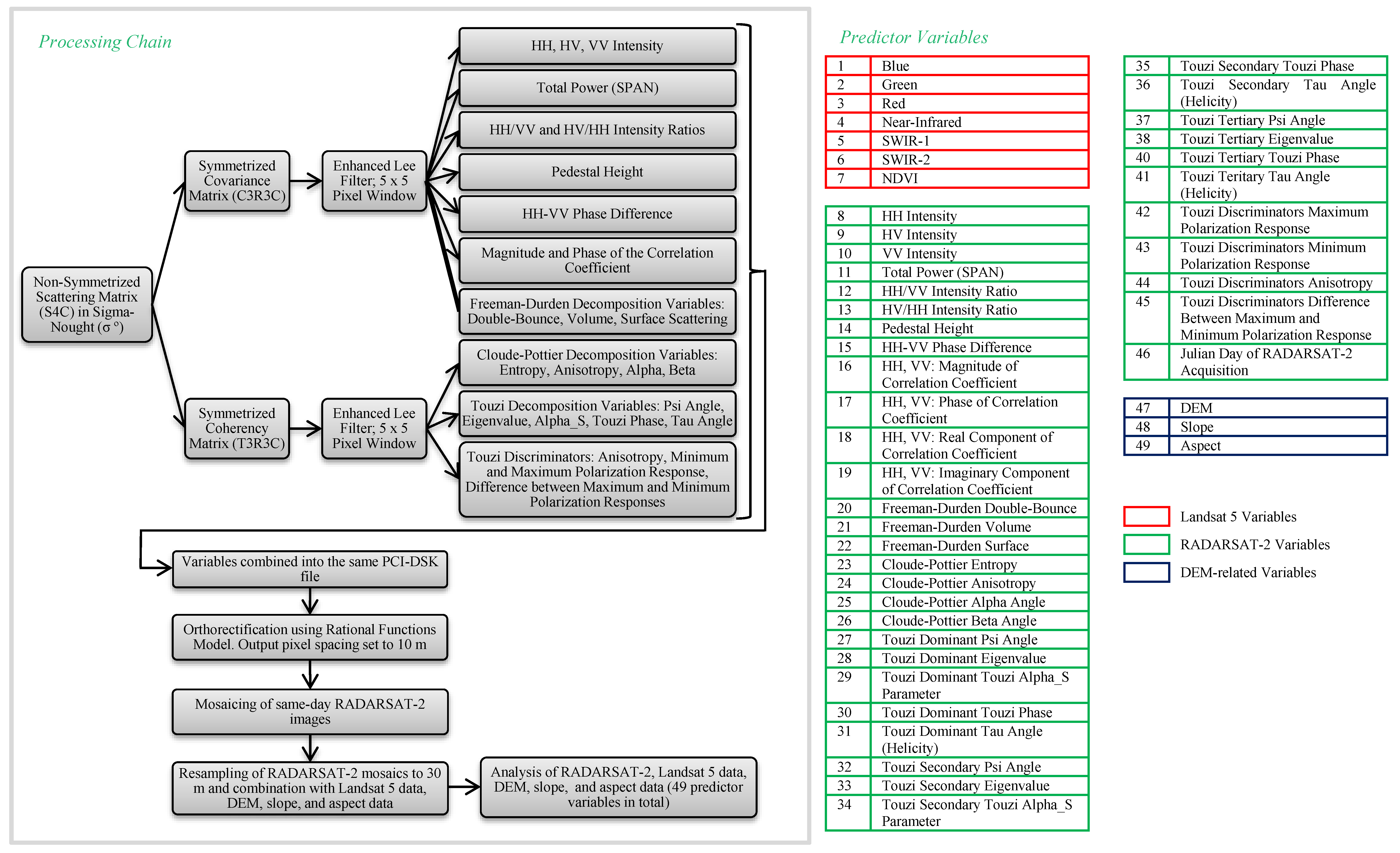
Variables included in the final, optimized dataset, as well as their respective importance values (averaged for all 10 model iterations) are presented in Table 8. Of the six spectral channels available with the Landsat 5 data, all but the blue channel were included. As was the case for all models generated in this research, the most important predictor variable was NDVI. This result is sensible since it was often difficult to distinguish between vegetated and un-vegetated classes in available SAR imagery. During the collection of field data many classes appeared to have comparable surface roughnesses (e.g., Tundra and Mixed Sediment), and moisture conditions could have also been similar or not detectable in available SAR imagery due to the acquisition of shallow versus steep incidence angle data, which tends to be more sensitive to differences in roughness than differences moisture [11]. This result is consistent with Demers et al. [13], who found that NDVI was instrumental in differentiating vegetated versus un-vegetated shoreline types. The DEM and slope were also important variables in this analysis. Baptist [71] found that classification of coastal features often improves with the inclusion of these data.

Table 8. Reduced set of predictor variables for an optimal Random Forest model, and their respective importance values for the Mean Decrease in Accuracy and Gini Index (importance values are based on averages generated from all 10 model iterations).

		Average Importance Value
		Mean Decrease in Accuracy	Rank of Variable (Most to Least Important)	Gini Index	Rank of Variable (Most to Least Important)
Landsat 5 Variables	Green	37.25	8	47.85	13
	Red	39.75	6	73.15	5
	Near-Infrared	39.35	7	88.91	3
	SWIR-1	36.79	10	82.64	4
	SWIR-2	40.62	4	91.89	2
	NDVI	68.94	1	119.90	1
RADARSAT-2 Variables	Freeman-Durden decomposition: double-bounce scattering	56.58	3	57.47	12
	Freeman-Durden decomposition: volume scattering	36.22	11	62.94	9
	Pedestal Height	31.31	14	65.26	7
	Touzi Decomposition: Secondary Eigenvalue	31.86	13	60.35	10
	Touzi Decomposition: Tertiary Eigenvalue	33.68	12	65.97	6
	HV Intensity	37.17	9	65.22	8
DEM Variables	DEM	57.82	2	60.28	11
	Slope	40.27	5	35.28	14

Table 8. Reduced set of predictor variables for an optimal Random Forest model, and their respective importance values for the Mean Decrease in Accuracy and Gini Index (importance values are based on averages generated from all 10 model iterations).

		Average Importance Value
		Mean Decrease in Accuracy	Rank of Variable (Most to Least Important)	Gini Index	Rank of Variable (Most to Least Important)
Landsat 5 Variables	Green	37.25	8	47.85	13
	Red	39.75	6	73.15	5
	Near-Infrared	39.35	7	88.91	3
	SWIR-1	36.79	10	82.64	4
	SWIR-2	40.62	4	91.89	2
	NDVI	68.94	1	119.90	1
RADARSAT-2 Variables	Freeman-Durden decomposition: double-bounce scattering	56.58	3	57.47	12
	Freeman-Durden decomposition: volume scattering	36.22	11	62.94	9
	Pedestal Height	31.31	14	65.26	7
	Touzi Decomposition: Secondary Eigenvalue	31.86	13	60.35	10
	Touzi Decomposition: Tertiary Eigenvalue	33.68	12	65.97	6
	HV Intensity	37.17	9	65.22	8
DEM Variables	DEM	57.82	2	60.28	11
	Slope	40.27	5	35.28	14

Several SAR variables were found to be of high importance to the model (Table 8). Of these, the Freeman-Durden double bounce parameter had the highest importance. Demers et al. [13] similarly observed that this variable was useful for detecting wetlands, and Ullmann et al. [17] found that double bounce intensity was related to vegetation density (low values were observed over sparser vegetation; high values were observed over denser vegetation). Banks et al. [12] observed that double bounce scattering was useful for differentiating wetlands from other vegetated land covers, and while double bounce values for all other classes were vastly different between their two study areas, values for wetlands at shallow angles were highly consistent. HV was the only SAR intensity channel included in the final, optimized set of 14 predictor variables (Table 8). Banks et al. [11] also found that compared to HH and VV, HV achieved the highest average class separability (based on the Bhattacharyya Distance) for multiple shoreline types [12]. Several SAR and optical variables achieved similar importance values, indicating a multi-sensor approach is optimal for this application. This is supported by the fact that Banks et al. [11] found low overall classification accuracies when attempting to classify shore and near-shore land cover types with SAR data alone, and found that their model required the combination of both SAR and optical data to distinguish sand from mixed-sediment beaches and flats.

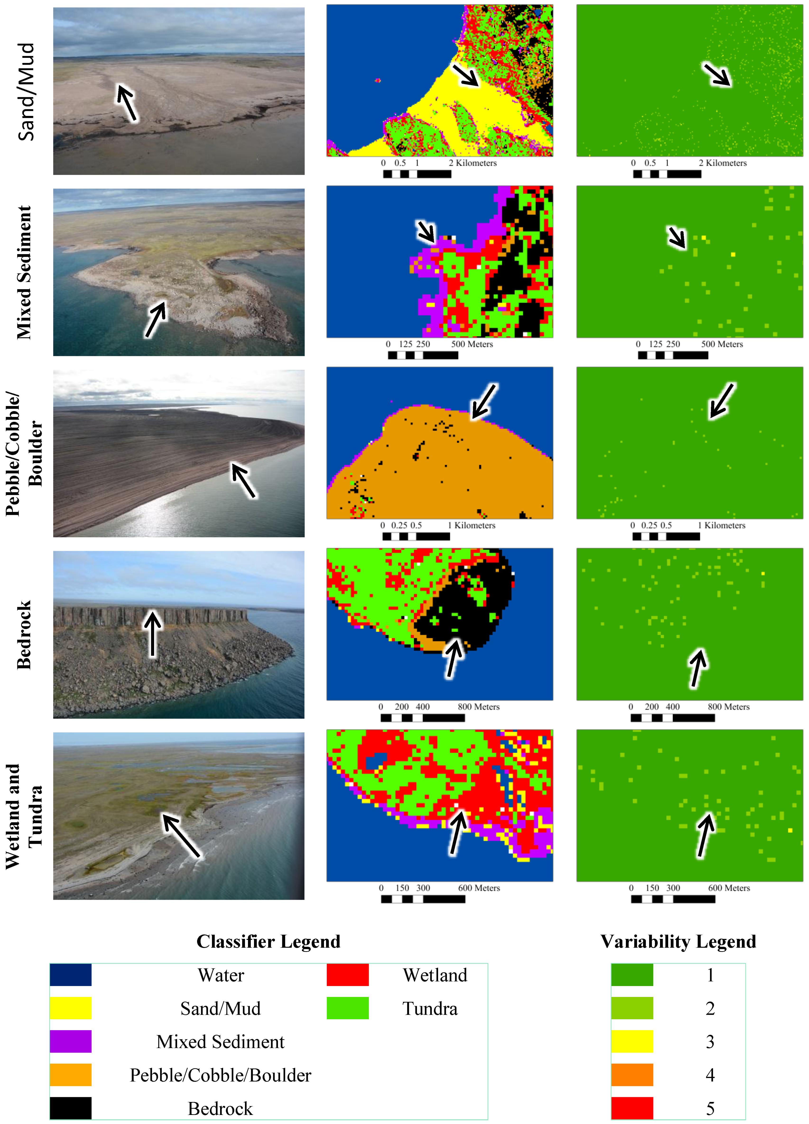
Classifier results for models generated with 14 predictor variables are presented visually in Figure 3, including outputs for the first model as well as variability of class predictions for all 10 model runs (i.e., the number of times a different class was predicted by one of the 10 models). Results show that while many areas are well classified, there is still potential for improvement. For example, some portions of the backshore containing pebbles and cobbles were misclassified as Bedrock (Figure 3; example for Mixed Sediment). This could be due to an insufficient number of training sites for that particular type of material, which could be of a similar roughness and colour as the bedrock types that were sampled [13]. This seems plausible since it was observed during the collection of field data that, in some cases, pebbles and cobbles were approximately as smooth as bedrock due to the size and arrangement or packing of materials. This is relevant with respect to the SAR data, since backscattering behaviour is affected by roughness, especially at shallow incidence angles [11,12].

In some cases Tundra was also misclassified as Wetland, though because wetlands are more sensitive to the effects of oiling this is not of major concern for the application of shoreline sensitivity mapping. This is because preference is always to avoid under-estimating the more sensitive class [8,13]. Demers et al. [13] also observed confusion between tundra and wetlands, which they suggested could be due to the misidentification of features during the training and or validation process, as both classes tended to transition into one another making it difficult to establish boundaries even in the field [72]. A similar observation was made in this research during the collection of training and validation data.

Though it is possible for Random Forest outputs to vary, despite models being generated with the same training data and set of predictor variables [25], this analysis has demonstrated potential for highly consistent results. Specifically, the last column of Figure 3 shows that the majority of each sub-scene was classified as the same land cover type by all 10 models. Other authors have observed highly variable outputs. Millard and Richardson [26] for example, found a high degree of variability between model iterations particularly along the edges of features. To compensate the authors ran 25 iterations of the same model and calculated probability values based on the number of times each model assigned the most commonly predicted class. As such, the degree of variability observed, may again depend on the particular dataset being tested.

OOBAs and independent accuracies were similar for all models generated in this test (differences ranged between 0% and 2%). This further demonstrates that with a sufficient training sample size it may be possible to utilize the internal accuracy assessments of Random Forest alone for model validation.

Figure 3. Field photos (left), classifier results for the first model generated with 14 predictor variables and 167 training points per-class (middle), and inter-model variability the number of times a different class was predicted by one of the 10 models (right). Values of 1 indicate no variability (all models predicted the same class) and values of 5 indicate the highest observed variability (five models predicted different classes at that pixel location). Approximately the same area in all three images is indicated by arrows.

Figure 3. Field photos (left), classifier results for the first model generated with 14 predictor variables and 167 training points per-class (middle), and inter-model variability the number of times a different class was predicted by one of the 10 models (right). Values of 1 indicate no variability (all models predicted the same class) and values of 5 indicate the highest observed variability (five models predicted different classes at that pixel location). Approximately the same area in all three images is indicated by arrows.

For this research, preference would have been to use training and validation data that was completely randomly distributed throughout the study area. Implementing this approach proved difficult in practice however, as analysts could not interpret the land cover types present at all locations, resulting in a large proportion of points being disregarded. As such we chose a purposeful sampling design, and while effort was still made to ensure some independence between training and validation data (e.g., each training/validation site was separated in space by a minimum of 100 m), it is still possible that the accuracies presented here are somewhat inflated as a result of optimistic bias [67]. Further study is required to fully address the degree to which this has affected classifier performance.

5.3. Potential for Remote Predictive Mapping

As was the case for test (1), three model iterations were deemed sufficient to represent the variability of outputs as only model accuracies and probabilities were assessed in this test. For each of the 15 models that were generated in total (three models each for the five different sets of training data), OOBAs, independent accuracies, Kappa statistic values, and per-class User’s and Producer’s accuracies for each iteration are provided in Table 9, and average probabilities for the winning class are provided in Table 10.

Results indicate that further study is required to fully assess the potential for spatial transferability of the model to areas without training data (Table 9). In all cases, models performed relatively well (OOBAs ranged from 89% to 92%, independent overall accuracies from 81% to 88%, Kappa statistic values from 0.77 to 0.86), though for each set of training data one or more land cover types tended to be poorly classified. The Class(es) that were poorly classified also varied between the different sets of training data. As an example, Bedrock was classified relatively well by all models except those that excluded data from survey 4 (User’s and Producer’s accuracies for the former were 71% and 74%; User’s and Producer’s accuracies for the latter were 33% and 7%). In contrast, Tundra was well classified by all models except those that excluded data from survey 3 (User’s and Producer’s accuracies for the former were 86% and 78%; User’s and Producer’s accuracies for the latter were 25% to 29% and 67%).

It is expected that the low accuracies observed in these cases are as a result of image-to-image variations in moisture conditions, differences in plant phenology, and for the substrate classes in particular (Sand/Mud, Pebble/Cobble/Boulder, and Bedrock) both differences in colour and in surface roughness. These are all likely to impact the consistency of SAR and optical image values in space and in time [60,61,62,63], which would make it more difficult to classify a given land cover type, especially if the full range of values exhibited throughout the study area are not well represented in the training dataset. This could explain why better accuracies were achieved when training data from all regions were included in the model, even if the sample size was relatively small (e.g., 13 to 25 points per-class, as was the case for test (1)).

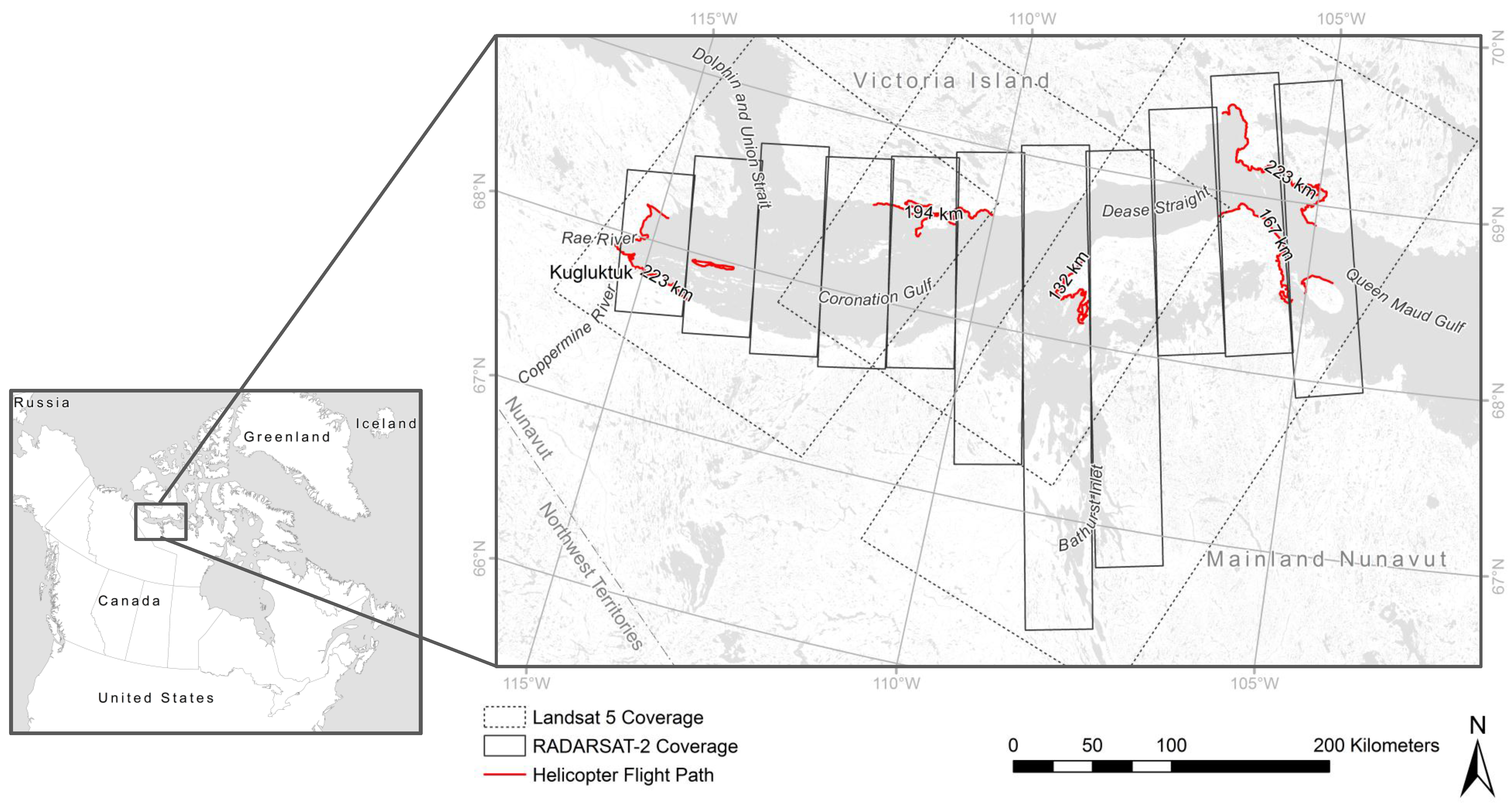
Table 9. OOBAs, independent overall accuracies, and Kappa statistic values, and per-class User’s and Producer’s accuracies (UA and PA) for Random Forest models generated with excluded training data from one in five videography surveys (numbered from west to east (see Figure 1)).

Survey Data Excluded From Model	Model Iteration	OOBA (%)	Independent Overall Accuracy (%)	Kappa Statistic	Water		Sand/Mud		Mixed Sediment		Pebble/Cobble/Boulder		Bedrock		Wetland		Tundra
					UA (%)	PA (%)	UA (%)	PA (%)	UA (%)	PA (%)	UA (%)	PA (%)	UA (%)	PA (%)	UA (%)	PA (%)	UA (%)	PA (%)
1	1	90	84	0.80	94	99	100	32	26	90	88	70	97	100	66	93	100	78
	2	89	84	0.80	96	99	100	32	25	90	88	70	97	100	66	93	100	78
	3	90	84	0.81	96	99	100	32	24	90	88	70	99	100	68	93	100	80
Number of Validation Sites					67		38		10		10		72		45		97
2	1	90	83	0.79	70	92	79	95	72	72	38	75	96	75	91	74	93	86
	2	90	83	0.80	71	94	81	95	72	72	38	75	96	75	91	74	93	86
	3	90	83	0.79	70	92	79	95	72	72	38	75	96	75	91	74	93	86
Number of Validation Sites					49		61		18		8		101		39		77
3	1	91	81	0.77	79	100	77	95	75	68	99	72	72	80	91	91	29	67
	2	92	81	0.77	79	100	77	95	74	68	99	72	73	80	94	91	25	67
	3	91	81	0.77	79	100	77	95	74	68	99	72	73	80	91	91	29	67
Number of Validation Sites					41		59		80		96		41		33		3
4	1	90	88	0.86	94	100	85	90	84	81	85	97	33	7	93	93	91	85
	2	90	88	0.86	94	100	85	90	84	81	86	97	33	7	93	92	88	86
	3	90	88	0.86	94	100	85	90	84	82	86	97	33	7	93	93	93	86
Number of Validation Sites					58		67		94		72		14		102		59
5	1	91	85	0.83	85	100	91	80	88	73	81	89	74	74	100	97	86	86
	2	90	85	0.82	85	100	91	80	89	71	79	89	74	74	100	97	86	86
	3	90	85	0.82	85	100	91	80	88	73	80	89	77	74	100	97	86	86
Number of Validation Sites					35		25		48		64		31		31		14

Table 9. OOBAs, independent overall accuracies, and Kappa statistic values, and per-class User’s and Producer’s accuracies (UA and PA) for Random Forest models generated with excluded training data from one in five videography surveys (numbered from west to east (see Figure 1)).

Survey Data Excluded From Model	Model Iteration	OOBA (%)	Independent Overall Accuracy (%)	Kappa Statistic	Water		Sand/Mud		Mixed Sediment		Pebble/Cobble/Boulder		Bedrock		Wetland		Tundra
					UA (%)	PA (%)	UA (%)	PA (%)	UA (%)	PA (%)	UA (%)	PA (%)	UA (%)	PA (%)	UA (%)	PA (%)	UA (%)	PA (%)
1	1	90	84	0.80	94	99	100	32	26	90	88	70	97	100	66	93	100	78
	2	89	84	0.80	96	99	100	32	25	90	88	70	97	100	66	93	100	78
	3	90	84	0.81	96	99	100	32	24	90	88	70	99	100	68	93	100	80
Number of Validation Sites					67		38		10		10		72		45		97
2	1	90	83	0.79	70	92	79	95	72	72	38	75	96	75	91	74	93	86
	2	90	83	0.80	71	94	81	95	72	72	38	75	96	75	91	74	93	86
	3	90	83	0.79	70	92	79	95	72	72	38	75	96	75	91	74	93	86
Number of Validation Sites					49		61		18		8		101		39		77
3	1	91	81	0.77	79	100	77	95	75	68	99	72	72	80	91	91	29	67
	2	92	81	0.77	79	100	77	95	74	68	99	72	73	80	94	91	25	67
	3	91	81	0.77	79	100	77	95	74	68	99	72	73	80	91	91	29	67
Number of Validation Sites					41		59		80		96		41		33		3
4	1	90	88	0.86	94	100	85	90	84	81	85	97	33	7	93	93	91	85
	2	90	88	0.86	94	100	85	90	84	81	86	97	33	7	93	92	88	86
	3	90	88	0.86	94	100	85	90	84	82	86	97	33	7	93	93	93	86
Number of Validation Sites					58		67		94		72		14		102		59
5	1	91	85	0.83	85	100	91	80	88	73	81	89	74	74	100	97	86	86
	2	90	85	0.82	85	100	91	80	89	71	79	89	74	74	100	97	86	86
	3	90	85	0.82	85	100	91	80	88	73	80	89	77	74	100	97	86	86
Number of Validation Sites					35		25		48		64		31		31		14

Table 10. Average classification probability for the winning class over all validation sites for Random Forest models generated with excluded training data from one in five videography surveys (numbered from west to east (see Figure 1)). Values for sites that were incorrectly classified were excluded from averages.

Survey Data Excluded From Model	Model Iteration	Water	Sand/Mud	Mixed Sediment	Pebble/Cobble/Boulder	Bedrock	Wetland	Tundra
1	1	0.98	0.71	0.74	0.72	0.87	0.91	0.79
	2	0.99	0.72	0.73	0.72	0.87	0.91	0.79
	3	0.99	0.71	0.74	0.72	0.87	0.91	0.79
2	1	0.99	0.93	0.81	0.93	0.85	0.85	0.81
	2	0.98	0.93	0.80	0.93	0.85	0.85	0.81
	3	1.00	0.93	0.81	0.94	0.85	0.85	0.80
3	1	1.00	0.97	0.70	0.86	0.84	0.82	0.71
	2	1.00	0.97	0.70	0.85	0.84	0.82	0.70
	3	1.00	0.97	0.70	0.85	0.84	0.82	0.70
4	1	0.98	0.86	0.72	0.89	0.83	0.81	0.80
	2	0.98	0.85	0.73	0.88	0.84	0.81	0.80
	3	0.98	0.85	0.73	0.88	0.84	0.81	0.80
5	1	0.98	0.82	0.72	0.90	0.91	0.85	0.83
	2	0.98	0.82	0.73	0.89	0.91	0.85	0.83
	3	0.98	0.82	0.72	0.89	0.91	0.86	0.83

Table 10. Average classification probability for the winning class over all validation sites for Random Forest models generated with excluded training data from one in five videography surveys (numbered from west to east (see Figure 1)). Values for sites that were incorrectly classified were excluded from averages.

Survey Data Excluded From Model	Model Iteration	Water	Sand/Mud	Mixed Sediment	Pebble/Cobble/Boulder	Bedrock	Wetland	Tundra
1	1	0.98	0.71	0.74	0.72	0.87	0.91	0.79
	2	0.99	0.72	0.73	0.72	0.87	0.91	0.79
	3	0.99	0.71	0.74	0.72	0.87	0.91	0.79
2	1	0.99	0.93	0.81	0.93	0.85	0.85	0.81
	2	0.98	0.93	0.80	0.93	0.85	0.85	0.81
	3	1.00	0.93	0.81	0.94	0.85	0.85	0.80
3	1	1.00	0.97	0.70	0.86	0.84	0.82	0.71
	2	1.00	0.97	0.70	0.85	0.84	0.82	0.70
	3	1.00	0.97	0.70	0.85	0.84	0.82	0.70
4	1	0.98	0.86	0.72	0.89	0.83	0.81	0.80
	2	0.98	0.85	0.73	0.88	0.84	0.81	0.80
	3	0.98	0.85	0.73	0.88	0.84	0.81	0.80
5	1	0.98	0.82	0.72	0.90	0.91	0.85	0.83
	2	0.98	0.82	0.73	0.89	0.91	0.85	0.83
	3	0.98	0.82	0.72	0.89	0.91	0.86	0.83

These results are comparable to those achieved by Demers et al. [13] who assessed the transferability of both pixel-based Maximum Likelihood and hierarchical object-based classifiers for shoreline sensitivity mapping. The authors similarly observed relatively high overall accuracies, with only one or two land cover types being poorly classified. While the focus of this analysis was not to compare Random Forest to object-based classification, it is worth noting that the latter approach has greater flexibility in terms of being able to make site-specific adjustments to the segmentation approach, as well as to the threshold values being used [73,74]. Demers et al. [13] theorized that this could improve results on a site-by-site basis, though this would require more user interference developing the model. While similar adjustments cannot be made to the Random Forest model produced in this research, it has been demonstrated that it is still possible to achieve accurate results with quality training data that better represents the full range of values for a given class.

6. Conclusions

This research has demonstrated the potential to classify shore and near-shore land cover types to acceptable levels (e.g., >~80%) using relatively few training samples (i.e., 25 points per-class). This result is relevant for mapping remote, Arctic shorelines since these areas are often difficult and expensive to access, and tend to make up only a fraction of the total image, which can make it harder to collect a large quantity of ground data. This result is also significant for mapping large areas since reducing the training sample size also decreases memory requirements and increases computational efficiency.

Where possible, it may still be reasonable to use more than the minimum required training samples, as it has also been demonstrated that increasing the training sample size also tends to increase classification accuracy and classifier probabilities. With a sufficient training sample size, it may also be possible to forego independent accuracy assessments, since it was found in this research that values can be comparable with the OOBAs provided by Random Forest.

In this analysis, the number of predictor variables used in the model could be greatly reduced without affecting model performance, including overall accuracy and classifier probabilities. Since using fewer predictor variables also increases computational efficiency and decreases data storage requirements, this result is relevant for mapping large areas. A final, optimized set of 14 predictor variables has also been defined that includes: all Landsat 5 spectral channels (except blue), NDVI values, Freeman-Durden double bounce and volume scattering, pedestal height, the secondary and tertiary eigenvalues of the Touzi decomposition, HV intensity, DEM values, and slope. While it is possible that a different set of predictor variables would achieve comparable or better results, these could be used as a basis for future shoreline mapping work, since it is probable that some or all of these would still be useful for classifying similar land cover types.

While accuracies of 91% were achieved when training data from the entire region were included in the model, mixed results were observed when assessing the potential for remote predictive mapping. This could be as a result of a combination of image-to-image variations in SAR and spectral values due to differences in moisture, roughness, and or colour, as well as from training samples not fully representing the range values a given class exhibits. When a variety of training data were included in the model, performance was improved, demonstrating that quality training data are required to achieve accurate results.

Using the conventional manual segmentation method, Environment Canada has only mapped approximately 6% of the ~162 000 km of shoreline contained within Arctic Canada [8,75]. With the methods developed in this research, there is potential to generate maps more efficiently if quality training data are available. These products could then provide at least some basis for oil spill response and contingency planning in other remote areas.