Article

In-Season Mapping of Crop Type with Optical and X-Band SAR Data: A Classification Tree Approach Using Synoptic Seasonal Features

Institute for Electromagnetic Sensing of the Environment, National Research Council (IREA-CNR), via Bassini 15, Milan 20133, Italy
*
Author to whom correspondence should be addressed.
Remote Sens. 2015, 7(10), 12859-12886; https://doi.org/10.3390/rs71012859
Submission received: 28 May 2015 / Revised: 22 September 2015 / Accepted: 24 September 2015 / Published: 30 September 2015
(This article belongs to the Special Issue Recent Advances in Remote Sensing for Crop Growth Monitoring)

Abstract

:
The work focuses on developing a classification tree approach for in-season crop mapping during early summer, by integrating optical (Landsat 8 OLI) and X-band SAR (COSMO-SkyMed) data acquired over a test site in Northern Italy. The approach is based on a classification tree scheme fed with a set of synoptic seasonal features (minimum, maximum and average, computed over the multi-temporal datasets) derived from vegetation and soil condition proxies for optical (three spectral indices) and X-band SAR (backscatter) data. Best performing input features were selected based on crop type separability and preliminary classification tests. The final outputs are crop maps identifying seven crop types, delivered during the early growing season (mid-July). Validation was carried out for two seasons (2013 and 2014), achieving overall accuracy greater than 86%. Results highlighted the contribution of the X-band backscatter (σ°) in improving mapping accuracy and promoting the transferability of the algorithm over a different year, when compared to using only optical features.

Graphical Abstract

1. Introduction

The increasing demand for information on crop acreage for agricultural monitoring in support of private and public decision makers requires the production of reliable crop maps [1,2]. Up-to-date information on agricultural land use is necessary for crop planning and management: e.g., for estimating biomass and yield, analyzing agronomic practices, assessing soil productivity, monitoring crop phenology and stress. Earth Observation (EO) techniques have been widely exploited in agriculture and agronomy for the advantages offered when compared to in situ and statistical surveys: frequency of acquisitions, synoptic view, and multi-dimensional content. Satellite remote sensing also constitutes the only source of consistent historical data for long-term analysis over large areas, e.g., for the identification of anomalous conditions in vegetation development driven by climatic variability [3]. Moreover, EO data are available already during the growing season, whereas official statistics on crop acreages are often provided at the end of the season or later, thus being not useful for supporting in-season crop management. Since crop productivity quickly responds to unfavorable growing conditions, timeliness in delivering information on crop status is an important operational requirement [4,5], e.g., for mitigating the impact of crop stress conditions, especially for summer crops, which are prone to water stress in the dry summer months [6,7].
EO satellite data have been used for agricultural monitoring since the launch of the Landsat-1 system in the early 1970s and their potential for distinguishing different crops has been shown across various environmental conditions, and with many different data sources and methodologies, e.g., in [8,9]. The Landsat archive constitutes the longest record of multi-spectral data available at medium spatial resolution, and has been used for crop mapping purposes at regional scale [10,11,12], using either spectral response and/or vegetation indices [13,14,15,16]. The opening of the Landsat archives in 2008 has pushed forward the implementation of data analysis and image classification techniques based on multi-temporal features and time series analysis [17]. Multi-temporal analysis techniques have been applied as well to coarser resolution data such as NOAA-AVHRR [18] and NASA-MODIS data [1,19], taking advantage of high revisit time for these sensors [20]. Other satellite data too, with spectral and spatial features similar to Landsat, have been used for crop mapping achieving satisfactory results, e.g., IRS LISS data [21,22].
Data acquired by Synthetic Aperture Radar (SAR) active sensors have also been exploited for crop mapping and monitoring, especially during the last two decades. C-band data have been used for mapping rice [23,24,25,26], wheat [27], and multiple crops [28,29,30,31,32]. L-band data have been used too, although with generally poorer performance [33,34]. More recently, with the launch of the TerraSAR-X and COSMO-SkyMed satellites, the use of X-band SAR data has largely expanded, mainly thanks to the higher spatial and temporal resolutions and theoretical flexibility of these platforms [35,36]. Concerning X-band SAR data, different polarimetric configurations have been tested for crop mapping, from vertical-based, e.g., in [37], to horizontal-based polarization, e.g., in [38]; comparative studies using multiple polarizations have been carried out as well, e.g., in [39]. However, to our knowledge no agreement has been reached so far on the best polarization configuration for crop mapping.
The integration of SAR and optical sensors for agricultural applications is a recent topic, aiming at reducing the impact of optical and SAR specific limitations (i.e., dependence on solar and clear sky conditions for the former, and on signal noise and stability for the latter). SAR and optical data integration takes advantage of their complementarity in terms of sensitivity to vegetation and soil characteristics [40,41,42]: plant biomass, soil moisture and surface texture for SAR, spectral response of canopy-background system and photosynthetic features for optical sensors [31,32,43]. Successful integration examples are the work of Michelson et al. [44], and more recently some large scale studies using multi-source data from RADARSAT-1, Envisat ASAR, SPOT and Landsat sensors [29,37,45,46]. The algorithms used for land cover mapping with both optical and SAR data range from maximum likelihood [46] and neural network ensembles [46,47] for crop classification, to maximum likelihood with iterated conditional modes [48] and Random Forest [49] for regional and urban land cover targets, up to fuzzy scores aggregation for burned area mapping [50]. With the advent of new generation satellites, e.g., Landsat 8, Sentinel-2, WorldView-3, as well as COSMO-SkyMed, TerraSAR-X, RADARSAT-2, and Sentinel-1, crop mapping applications can be more timely and reliable, in particular during the early growth stages, and the operational use of such techniques will be promoted.
This paper describes a classification tree approach for in-season crop mapping, which exploits features derived from multi-temporal optical, Landsat 8 Operational Land Imager (OLI), and X-band SAR, COSMO-SkyMed, data for producing reliable in-season crop maps over temperate areas. The proposed approach builds on the analysis of separability between different crops to identify the best performing proxy combinations and synoptic seasonal features as crop mapping inputs. Classification tree approaches can handle input features of different types and derived from different sources, and are directly interpretable and adaptable, being structured as a set of simple rules [51,52,53]. These characteristics make classification tree approaches both efficient and effective, especially for delivering mapping algorithms which are to be used in operational contexts.
The main objective is to define a classification tree approach for producing a crop map early in the summer season, i.e., around mid-July [54], to support agricultural management in Northern Italy. Spectral features for the winter and summer crop seasons (named synoptic seasonal features) are extracted from the temporal profiles of a set of proxies derived from optical and SAR data. Different proxies were used, sensitive to vegetation and soil conditions and able to characterize the dynamics of different crop types throughout the growing season: Spectral Indices (SIs) from optical data and/or backscatter and interferometric coherence information from X-band SAR data. Most of the literature using multi-temporal information for crop mapping focus on the use of temporal profiles of spectral indices derived from optical data [55,56,57,58], and only recently some authors successfully included SAR backscatter profiles for rice mapping [59,60]. The novelty of our work are the use of synoptic seasonal features integrating optical and SAR data, and the delivery of crop type mapping already during the early stage of growth; eventually, the transferability to a growing season different from the one used for developing the approach is tested.

2. Materials

2.1. Study Area

The study area is located in Lombardy region, northern Italy (Figure 1); it lies south of Milan and it is bordered by the Po river. The area, covering around 1100 Km2, is mostly flat and intensively cultivated. Climate is continental, with annual temperature changes between January and July up to 20 °C and average precipitations of 850 mm/year. The most economically valuable crop types cultivated in Lombardy are (in per cent of total cropland area): maize (38.5%), temporary and permanent meadows used for forages (34.1%), rice (10.1%), winter cereals (wheat and barley, 7.5%), soybean and other legumes (2.7%), and vegetables (1.4%) [61]. The two major crop seasons run from October to June and from April to October for winter and summer crops, respectively. Barley is the prevailing winter crop, typically flowering in April-May and harvested in May-June. The main summer crops, covering most of the cropland area and consuming most of irrigation resources, are maize and rice. Maize, sown between April and early May, reaches the peak of the vegetative phase in July and is harvested from the end of August through September. Maize is often also sown in double cropping practices for fresh forages or silage, after meadows or winter cereals, in integrated crop-livestock systems. Rice is usually sown later than maize, from the second half of April to late May, reaching the flowering stage in late July or early August, and it is harvested from late September onwards.
Figure 1. The study area in Northern Italy and an overview of the optical and SAR data coverage: (a) Landsat 8 OLI, path 194-rows 28-29 (03 July 2014, RGB = 543), (b) Landsat 8 OLI, path 193-rows 28-29 (10 June 2014, RGB = 543), (c) COSMO-SkyMed-1 (10 July 2014, Product processed under a license of the Italian Space Agency (ASI); Original COSMO-SkyMed Product - ©ASI - (2013)).
Remotesensing 07 12859 g001

2.2. Satellite Data

The remotely sensed dataset is composed of 13 COSMO-SkyMed (CSK) and 14 Landsat 8 OLI images covering the spring/summer seasons of the years 2013 (18 April–23 July) and 2014 (05 April–19 July), as shown in Table 1. CSK data have been consistently acquired by the same satellite of the COSMO SkyMed constellation (CSK 1) in single polarization (HH) and interferometric mode. CSK dataset of both years is acquired from the same flight track and with constant orbital configuration. This configuration allowed us to exploit the dataset not only for X-band intensity calculation, but also for extracting repeat-pass interferometric coherence, with absolute values of perpendicular baselines ranging from 190 to 479 m for 2013 CSK dataset, and from 363 to 1020 m for 2014 CSK dataset.
Table 1. The X-band SAR and optical satellite acquisitions divided into the development (2013) and the transferability dataset (2014).
DatasetSAR Data (COSMO SkyMed-1)Optical Data (Landsat 8 OLI)
DateDOYDateDOYWRS-2 (path/rows)
201318-0410813-05133194/28-29
04-0512407-06158193/28-29
20-0514014-06165194/28-29
05-0615623-06174193/28-29
21-0617230-06181194/28-29
07-0718816-07197194/28-29
23-07204
201405-049514-04104194/28-29
21-0411123-04113193/28-29
07-0512709-05129193/28-29
23-0514325-05145193/28-29
08-0615901-06152194/28-29
10-0719110-06161193/28-29
03-07184194/28-29
19-07200194/28-29
The CSK product was acquired as StripMap HIMAGE in Single Look Complex (SLC) format, HH polarization, descending pass, with look angle of 24.1 degrees. The OLI dataset was collected by taking advantage of two overlapping WRS-2 paths (193 and 194, rows 28-29) that guarantees a theoretical revisiting frequency of 7–9 days over the study area. Landsat 8 OLI scenes were retained only when overall cloud cover was less than 10%.

2.3. Reference Data

Three thematic levels of crop types were considered for covering the variability of crops cultivated in the study area: a detailed level (level 2—Lev2), an intermediate level (level 1—Lev1), and a generic level (level 0—Lev0), as summarized in Table 2. Lev2 is composed of 12 classes: early maize (Ma1), medium maize (Ma2), late maize (Ma3), early rice (R1), late rice (R2), dry seeded rice (R3), early soybean (Sb1), late soybean (Sb2), winter crop (WC), double crop (i.e., winter crop followed by a summer crop; DC), forages (i.e., permanent and temporary meadows used as fodder; Fo), and forestry-woodland (either natural or man-made; F-W). Lev1 groups the subclasses of maize, rice and soybean crops into three mono-type classes: maize (Ma), rice (R), and soybean (Sb), thus delivering a total of 7 crop cover classes (Ma, R, Sb, WC, DC, Fo, F-W). Indeed, Lev1 classes represent the target crop types for operational use of the early crop map, but since some Lev1 classes showed multimodal SIs temporal profiles due to different sowing dates of various cultivars (e.g., long and short cycle maize), we split some summer crop classes into different sub-classes in order to effectively calculating class separability, thus composing Lev2 classes. Finally, Lev0 was derived by further aggregating summer crop types (Ma, R, Sb) into a unique summer crop (SC) class, leading to a total of 5 land cover classes (SC, WC, DC, Fo, F-W).
Table 2. Composition of the reference sample for 2013 development set, including training and validation sub-samples.
Lev2Lev1Lev0
Crop ClassTraining px/fieldsValidation px/fieldsCrop ClassTraining px/fieldsValidation px/fieldsCrop ClassTraining px/fieldsValidation px/fields
Ma1maize (early seeding)881/34520/17Mamaize2233/961173/48SCsummer crop (generic)5439/2602794/130
Ma2maize (medium seeding)771/36378/18
Ma3maize (late seeding)581/26275/13
R1rice (early seeding)628/34335/17Rrice2296/1121066/56
R2rice (late seeding)962/44431/22
R3rice (dry seeding)706/34300/17
Sb1soybean (early seeding)462/26319/13Sbsoybean910/52561/26
Sb2soybean (late seeding)448/26242/13
WCwinter crop782/30344/15WCwinter crop782/30344/15WCwinter crop782/30344/15
DCdouble crop1007/34443/17DCdouble crop1007/34443/17DCdouble crop1007/34443/17
Foforages (artificial grassland)447/22212/11Foforages (artificial grassland)447/22212/11Foforages (artificial grassland)447/22212/11
F-Wforestry-woodland1118/34530/17F-Wforestry-woodland1118/34530/17F-Wforestry-woodland1118/34530/17
For building the reference dataset to be used for crop type classification implementation, a set of 570 crop fields (almost 9000 pixels), belonging to 12 different crop classes, have been identified for the 2013 spring-summer season based on the Annual Agricultural Land Use Map of Lombardy region (Carta Uso Agricolo Annuale, CUAA); this map is produced and distributed by the “Ente Regionale per i Servizi all’Agricoltura e alle Foreste” (i.e., the regional agency for agriculture and forest services of the Lombardy regional government) on an annual basis and relies on farmers’ declarations as the primary source of information [62].
The crop categories of the CUAA legend are not consistent with crop classes defined on the basis of spectral response from remotely sensed data. For example, the CUAA crop category “maize” includes both single and double crop cultivations, which are characterized by different temporal profiles of the Spectral Indices derived from OLI data, thus leading to two distinct classes. Furthermore, the CUAA category “forages” includes all crops cultivated for animal consumption, i.e., some winter cereals, fodder and managed grasslands (alfalfa and similar), which are grown and mowed several times per season. Finally, no official figures are provided for the accuracy of the CUAA product. Therefore, the CUAA 2013 map was not used as direct reference data source, but it was used as base information for extracting sample fields, which have been confirmed by visual assessment of high resolution satellite photos covering part of the study area (acquired on 22 March and 10 August 2013, from Google Earth), in situ observations for a limited number of fields (survey along main roads using camera and GPS) and interpretation of multi-temporal profiles of optical scenes (i.e., for extracting Lev2 subclasses from Lev1 by assessing season timing of EVI peak, and for delineating double cropped fields).The reference dataset for 2013 growing season is described in Table 2, including the number of fields sampled for each class and level. The sampling was done on the basis of random selection of spatially distributed points from CUAA 2013 map within each crop class, followed by checking for correct class labelling consistently with semantic crop classes included into our target legend. Finally, a subdivision of the reference set was made on a per-field basis, with 2/3 of the fields used for training and 1/3 used for validation (see Table 2). This procedure allowed the attribution of crop type labels consistent with target crop classes in 2013 season, and it is used together with the satellite development set. For 2014 season, a validation set was constructed starting from CUAA 2014 map and using the same checking procedure described for 2013 reference set. 2014 validation set is composed of a total of 3759 pixels, with class cardinality ranging from 289 to 753 pixels, and it is consistently used for assessing mapping accuracy derived from satellite transferability set.
The satellite and reference data have been divided into two separate datasets: (i) a development set, used for best input feature selection, training of the classification algorithm and accuracy assessment (i.e., for developing the crop mapping approach), made of the satellite data from the year 2013 (7 CSK, 6 OLI) and the training and validation samples extracted and checked from CUAA 2013 (Table 2) and (ii) a transferability set, used for validation of the crop mapping approach implemented for a different growing season (i.e., testing the transferability of the approach), composed of the satellite data acquired in 2014 (6 CSK, 8 OLI) and the validation sample extracted and checked from CUAA 2014.

3. Methods

3.1. Satellite Data Pre-Processing

Landsat 8 OLI data [63] were converted to surface reflectance through atmospheric correction, performed with Atmospheric/Topographic CORrection for Satellite Imagery (ATCOR) [64]. Multi-temporal SIs have already demonstrated their efficacy in capturing cropland characteristics [54,65]. For our approach, three SIs were derived as proxies of crop conditions from optical data: Enhanced Vegetation Index (EVI, Equation (1)), Normalized Difference Flood Index (NDFI, Equation (2)), and Red Green Ratio Index (RGRI, Equation (3)).
EVI = 2 ρ NIR(b5OLI) ρ RED(b4OLI) ρ NIR(b5OLI) + RED(b4OLI) 7 .5ρ BLUE(b2OLI) + 1
NDFI = ρ RED(b4OLI) ρ SWIR(b7OLI) ρ RED(b4OLI) + ρ SWIR(b7OLI)
RGRI = ρ GREEN(b3OLI) ρ RED(b4OLI)
EVI was developed as an enhanced version of NDVI, including correction for background and atmospheric disturbances; the spectral bands of near infrared (NIR) and visible red (RED) are supplemented by information from the visible blue (BLUE) band, by using optimal weighting [66]. EVI provides information about vegetation vigor, linked to biomass and fractional cover. As a complement to EVI, we included NDFI, which is an index developed for the detection of surface water in flooded rice areas; NDFI, originally introduced as NDFI2 or NDSIB2B7 [67], is the normalized difference of the RED and the short wave (SWIR, 2.1–2.2 µm) spectral bands. NDFI provides information about soil moisture and flooding conditions, especially relevant for paddy rice fields. The ratio of the RED and GREEN reflectance values (RGRI) was included due to its sensitivity to photosynthetic efficiency and leaf pigments [68].
Figure 2 shows EVI (a) and NDFI (b) multi-temporal profiles extracted from the 2014 OLI dataset (covering the whole growing season: 16 March–23 October), together with acquisition dates of CSK and OLI for the development dataset (2013); the grey bar highlights the temporal range adopted as early crop map production deadline (mid-July). The profiles qualitatively well describe the cycles of the major winter and summer crops of the study area, thus promoting the SIs selected as suitable candidates for monitoring crop dynamics during the season.
CSK images were pre-processed with MAPscape-RICE software [59] for (i) mosaicking single frames into slant range continuous strips and (ii) co-registration of images using orbital information and automatic spatial matching based on cross-correlation.
Two different proxies of crop conditions were derived from CSK data: X-band backscattering coefficient sigma nought (σ°), related to plant biomass and morphology and soil conditions (moisture and roughness), already used for crop mapping by Fontanelli et al. [69], and repeat-pass interferometric coherence (γ), related to the evolution of surface scattering properties of canopy/background system (plant height and density) during the season [70,71]. The σ° was derived through three processing steps: (a) multi-temporal speckle filtering according to the approach developed by De Grandi et al. [59,60,72], to balance differences in reflectivity between images at different times, (b) geocoding and radiometric calibration, using a Digital Elevation Model (SRTM DEM, at 90m equivalent ground resolution) and the radar equation, in which scattering area, antenna gain patterns and range spread loss were considered, and finally (c) normalization on local incidence angle, according to the cosine law. The interferometric coherence γ maps were produced using the complex data of image pairs of consecutive acquisitions [73], with a temporal baseline of 16 days (32 days for the 08 June–10 July 2014 pair). The multi-temporal σ° and γ maps were finally geocoded to UTM 32N WGS84 and spatially resampled to the same spatial resolution of L8 OLI images (30 m), by aggregating the average value of 10 × 10 pixels at the original resolution of 3 m.
Figure 2. EVI (a) and NDFI (b) multi-temporal profiles extracted from the 2014 OLI dataset for major crops in Lombardy study site (covering the whole growing season from winter crop stem elongation phase to summer crops harvesting: March to October). Satellite acquisition dates of OLI and CSK images used for the development set (2013) are superimposed on the graphs. Grey color box represent the target temporal range for producing the early in-season crop map (i.e., mid-July).
Remotesensing 07 12859 g002

3.2. Multi-Temporal Proxies Test

In order to capture the distinct seasonal patterns of different crops, we divided the multi-temporal dataset into two periods: (i) from April to the beginning of June, when winter crops are harvested; and (ii) from May-June, when summer crops emergence starts, to mid-July. Synoptic seasonal features over the two periods were computed for EVI, RGRI, σ° and γ. For NDFI, only pre-summer features were derived, being it related to flooding in rice cultivation. Seasonal proxies used for the development set (2013) are summarized in Table 3. Each seasonal proxy is made a series of values corresponding to dates falling into the Day Of Year (DOY) range representative of winter crop and early summer crop seasons.
For each proxy, the following synoptic seasonal features were extracted for the winter and summer periods: minimum value over the seasonal range (min), maximum value over the seasonal range (max), mean value over the seasonal range (ave), standard deviation over the seasonal range (std) (Figure 3), and the asymmetry index of the seasonal proxy scores histogram, or skewness (ske), not included in Figure 3.
Table 3. Optical and X-band SAR seasonal proxies for the 2013 development set. EVIW = EVI in winter crop growing season; EVIS = EVI in early summer crop growing season; RGRIW = RGRI in winter crop growing season; RGRIS= RGRI in early summer crop growing season; NDFI = NDFI before summer crop peak; σ°W = X-band HH backscatter in winter crop growing season; σ°S = X-band HH backscatter in early summer crop growing season; γW = interferometric coherence in winter crop growing season; γS = interferometric coherence in early summer crop growing season.
Seasonal ProxyDOY Range (2013 Dataset)Crop Vegetation and Soil Characteristics Connected
EVIW133–165EVI during winter crop peak season (May–June)
EVIS174–197EVI during early summer crop growth season (June–July)
RGRIW133–165RGRI during winter crop peak season (May–June)
RGRIS174–197RGRI during early summer crop growth season (June–July)
NDFI133–197NDFI before summer crop peak (May–July)
σ°W108–156X-band backscattering coefficient during winter crop peak season (May–June)
σ°S172–204X-band backscattering coefficient during early summer crop growth season (June–July)
γW108–156repeat-pass interferometric coherence during winter crop peak season (May–June)
γS172–204repeat-pass interferometric coherence during early summer crop growth season (June–July)
Figure 3. An example of synoptic seasonal features (min, max, ave, std) extracted for the winter and summer periods from EVI 2014 multitemporal profiles (April to mid-July) over winter wheat (red) and maize (yellow) sample fields.
Remotesensing 07 12859 g003

3.3. In-Season Crop Type Classification

The classification scheme and the input features were selected to satisfy as much as possible crop mapping pre-operational requirements, thus (i) providing a product with high thematic mapping accuracy; (ii) being transferable to different years and (iii) building on rules both simple and interpretable, even to those who are non-experts in pattern recognition and remote sensing. Given these constraints, we implemented a rule-based classification tree, which grants both flexibility and robustness, and support the use of multi-source data [51,52,53]. The scheme is implemented using the Classification and regression Tree (CT) algorithm, in the extension of J48 java routine, programmed in WEKA 3.6 [74]. J48 CT routine is shaped on C4.5 [75] and consists of a recursive algorithm, that generates a classification tree through iterative partitioning of the feature space by using the information gain (computed from the entropy function) of each attribute for a set of cases [76]. Each node in a tree is associated to a set of two or more cases. The attribute with the highest information gain is selected for each node, and the optimal threshold for continuous attributes is computed. For avoiding too complicated tree structures and over-fitting, embedded pruning capabilities are implemented into J48 CT algorithm, according to a given confidence level. For our J48 CT implementation we allowed only binary splits for each node, and used online pruning, with confidence factor of 0.25 and sub-tree raising option. For dealing with possible over-fitting and minimizing the tree size, we set the minimum number of classified instances per each final node equal to 200, which is approximately half of the size of the smallest Lev1 crop class in the training dataset (forages, 447 pixels, see Table 2). CT outputs a set of hierarchical rules with optimized decision boundaries in form of thresholds, which can be straightforwardly implemented for image classification. An additional output of CT is the assessment of class attribution error for each tree node, which is a useful metric for ex-post tree re-structuring, in case of high accumulation of misclassified instances in some branches.
The performance of the CT schemes implemented was tested with different combination of proxies and features, by computing the confusion matrix and derived accuracy metrics [77]. During this phase, results achieved with the CT approach were compared to the ones achieved by Random Forest (RF) classification [78], which is currently acknowledged as the upper limit reachable using state of the art classification tree algorithms and multi-source data [79,80,81].

3.4. Selection of Input Features

Descriptive statistics were extracted for each Lev2 class and different synoptic seasonal features combinations: (i) σ° features; (ii) σ° and γ features; (iii) EVI features; (iv) EVI and NDFI features; (v) EVI, NDFI and RGRI features; (vi) EVI, NDFI, RGRI, and σ° features; (vii) EVI, NDFI, RGRI, σ° and γ features. Lev2 class-by-class separability was computed for these combinations using the Jeffries-Matusita Distance (J-MDIST) [82], and aggregated as per-class separability by averaging all possible pairings comprising a specific class. As a rule of the thumb, good separability is generally set at J-MDIST higher than 1.9 [83]. Lev2 classes used for extracting class-by-class separability were further summarized into average class separability scores at Lev1. The best performing combinations of seasonal proxies were then selected by maximizing separability, with J-MDIST~2. Following the selection of best proxy combinations, the feasibility of reducing the synoptic seasonal features input set was assessed based on the overall performance of preliminary crop classification tests using CT and RF, with three different sets of features: (i) minimum, maximum, mean, standard deviation, and skewness (min-max-ave-std-ske); (ii) minimum, maximum, and mean (min-max-ave); and(iii) minimum and maximum (min-max). The rationale behind this choice is to assess the effect in terms of mapping accuracy, when discarding features mostly affected by year-to-year variability of satellite image frequency: i.e., we first excluded standard deviation and skewness, and then the average, which in case of few scenes available can be more biased than extreme values (min-max).
At the end of the test phase, we retained the input set (i.e., the combinations of proxies and synoptic seasonal features) that granted as much reduction as possible in the number of features, granting the lowest difference of overall accuracy between CT and RF results, at Lev1.

3.5. Validation

The CT scheme derived for the selected input set was applied and validated over 2013 and 2014 seasonal data, development and transferability sets, by calculating confusion matrices and derived metrics: Overall accuracy (OA), Kappa coefficient of agreement (κ) and per-class Commission (CE) and Omission (OE) Errors [77]. Validation was carried out on samples independent from the training set, with per-class cardinality either proportional to the one of the training set (case t), or of actual cropland cover calculated from CUAA reference information (case r). Crop mapping performance was assessed at two thematic levels: Lev1, and Lev0.
An overview of the whole methodological approach described in Section 3 is given in Figure 4.
Figure 4. Flow chart of the overall methodological approach.
Remotesensing 07 12859 g004

4. Results and Discussion

4.1. Selection of Synoptic Seasonal Features

Since the separability scores for Lev2 classes were generally not high enough for expecting good performance in early mapping, Lev1 (i.e., 7 crop classes) was chosen as the target level for our crop mapping approach. Class separability scores aggregated at Lev1 (Table 4) show some interesting response to the different input proxy combinations (derived from optical and/or X-band SAR data).
Using only X-band SAR information, J-MDIST increases consistently for all classes when adding γ to σ°: from +0.041 for better separated classes (rice and forages), to +0.150 and up to +0.204 for crop classes difficult to separate using only σ° (maize, soybean, and double crop). Using optical proxies, a slighter but consistent increment in J-MDIST (0.037 to 0.053) is observed by adding NDFI to EVI for summer crops (maize, rice, and soybean). Further addition of RGRI brings a small, yet consistent, increment in J-MDIST (0.009 to 0.023) over summer crops. As regards separability achieved by using optical and SAR proxies together, an increment is observed adding σ° to the full optical feature set; since separability is already close to the maximum value (J-MDIST~2) the increment is lower for maize and soybean classes (+0.007 to +0.010). No significant increment (+0.000 to +0.002) is granted by further adding γ.
Based on separability scores shown in Table 4, we kept only the best performing combinations in terms of overall separability (minimum JMDIST > 1.98): EVI+NDFI+RGRI (ERN, J-MDIST > 1.983) and EVI+NDFI+RGRI+σ° (ERN+s, J-MDIST > 1.997). Since the scores achieved using EVI+NDFI+RGRI+σ° and EVI+NDFI+RGRI+σ°+γ synoptic features are not significantly different, we decided to discard the combination including γ to keep the feature set as simple as possible. These two combinations were used as input for the classification approach development.
Table 4. Mean J-MDIST for each crop type class at Lev1, as a function of the combination of OLI and SAR proxies. Maximum separability corresponds to J-MDIST = 2.
Crop Type (Lev1)Combination of Seasonal Proxies Used
σ°σ°+γEVIEVI+NDFIEVI+NDFI+RGRIEVI+NDFI+RGRI+σ°EVI+NDFI+RGRI+σ°+γ
Maize1.7811.9441.9281.9731.9881.9981.999
Rice1.9361.9771.9511.9881.9972.0002.000
Soybean1.7841.9341.9071.9601.9831.9971.999
Winter crop1.9211.9881.9981.9991.9992.0002.000
Double crop1.7551.9591.9981.9991.9992.0002.000
Forages1.9491.9901.9992.0002.0002.0002.000
Forestry-woodland1.9271.9901.9992.0002.0002.0002.000
Table 5 shows OA of preliminary crop classification tests using synoptic seasonal features extracted from ERN and ERN+s combinations at Lev1 and Lev0 as input for CT, with RF scores as reference. Results achieved with the complete features set (min-max-ave-std-ske) show that: (i) at Lev1, OA achieved with CT increases from 85.3% (ERN) to 89.0% (ERN+s), with a gap towards RF of 5.8%–8.9%; (ii) at Lev0, very high OA is scored by CT (96.7–97.8%), reducing the gap towards RF to 1.3%–2.5%. Reducing the input features to min-max-ave set did not produce a sensible decrement in OA, with maximum decrement in OA of −0.8% across different proxy combinations and thematic levels, while increments in OA for CT are observed using ERN: +1.2% (at Lev0) and +1.7% (at Lev1). Further reducing input features to min-max did not significantly change OA at Lev0, but a decrement up to 2.1% was observed for Lev1.
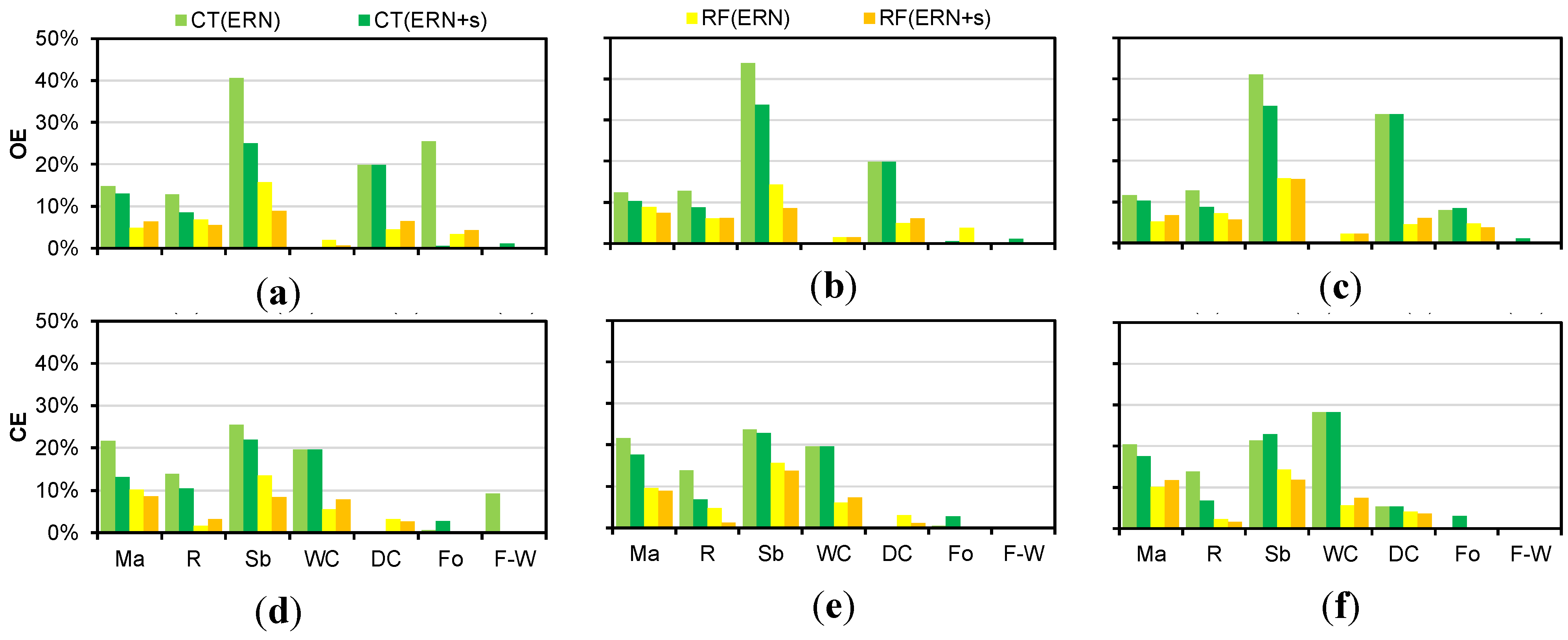
Figure 5 shows per-class omission and commission errors (OE and CE) at Lev1 for CT and RF. When the min-max-ave set is used, no significant increase of per-class errors is observed, compared to the use of a full set of features (min-max-ave-std-ske; Figure 5b–e). Instead, the use of min-max-ave set and CT fed with optical only features (ERN) contributes to a reduction of OE for forages (25%, Figure 5b), and of CE for forestry-woodland (9%, Figure 5e). When the input feature set is further reduced to min-max (Figure 5c–f), higher errors for double crop (+11% OE, +5% CE), and some overestimation of winter crop (+8% CE) are observed. The best performing synoptic seasonal feature set was therefore identified as min-max-ave, which was therefore selected as best option input for early crop mapping.
Figure 5. Per-class omission (OE) and commission (CE) errors for Lev1 classes achieved by CT with ERN and ERN+s proxies and different synoptic seasonal feature sets: (a) OE with min-max-ave-std-ske; (b) OE with min-max-ave; (c) OE with min-max; (d) CE with min-max-ave-std-ske; (e) CE with min-max-ave; (f) CE with min-max. Ma = maize; R = rice; Sb = soybean; WC = winter crop; DC = double crop; Fo = forages; F-W = forestry-woodland; ERN = EVI+NDFI+RGRI; ERN = EVI+NDFI+RGRI+σ° = ERN+s. Results achievable using RF are shown as reference.
Remotesensing 07 12859 g005
Table 5. Overall Accuracy (OA) for CT at Lev1 and Lev0, using ERN and ERN+s proxy combinations and min-max-ave-std-ske, min-max-ave and min-max seasonal features. ERN = EVI+NDFI+RGRI; ERN = EVI+NDFI+RGRI+σ° = ERN+s. Results achievable using RF are shown as reference.
OAERNERN+s
MethodLevelmin-max-ave-std-skemin-max-avemin-maxmin-max-ave-std-skemin-max-avemin-max
CTLev185.3%87.0%84.8%89.0%88.7%86.9%
Lev096.7%97.9%96.4%97.8%97.8%96.2%
RF (reference)Lev194.2%93.4%93.9%94.8%94.6%93.8%
Lev099.2%99.2%99.1%99.1%99.3%99.0%

4.2. In-Season Crop Type Classification

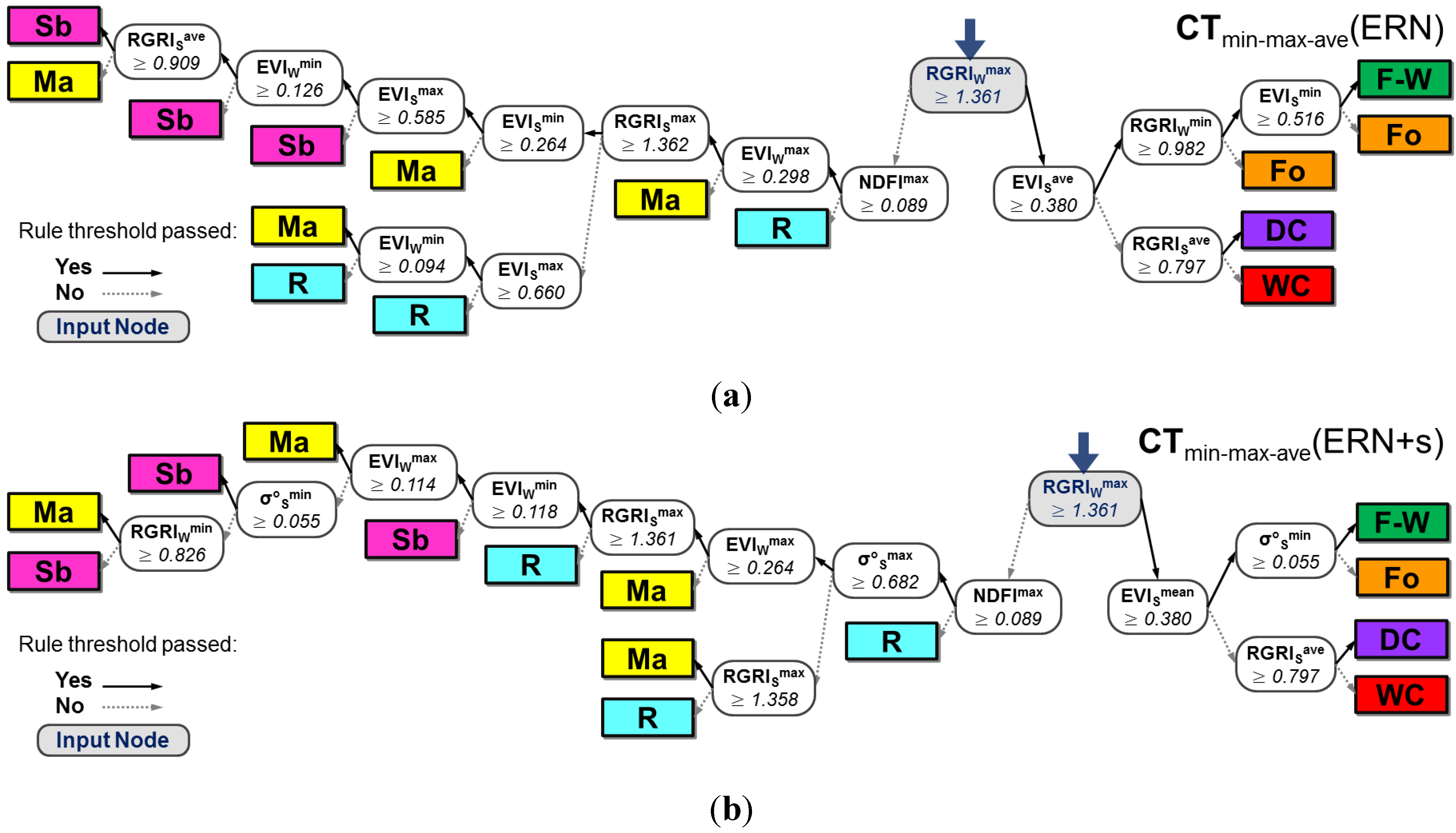
Figure 6 shows the two CT schemes implemented using the J48 algorithm for to the 2013 training dataset with the min-max-ave synoptic seasonal feature set, applied to the ERN (CTmin-max-ave(ERN), Figure 6a) and ERN+s (CTmin-max-ave(ERN+s), Figure 6b).
The CT scheme developed using only optical features (CTmin-max-ave(ERN)) shows the first split of tree nodes based on winter season RGRI maximum (RGRIWmax ≥ 1.361), separating pixels which are vegetated in May-June (right side) from non-vegetated ones (left side), thus distinguishing summer crops from winter crops, double crops and other agricultural land cover. The tree branches on the right side of Figure 6a further split winter and double crops from non-sown land covers (forages, forestry-woodland) based on two combinations of EVI mean in early summer (EVISave), since the latter classes show high green fractional cover already during spring, when summer crops are not yet sown. All these nodes show crop type attribution errors lower than 2.4%, except for winter crop class (9.6% cumulated node error). Left branches in Figure 6a are populated by summer crop classes, characterized by low RGRIWmax. Below these branches, the main splits are based on NDFI maximum (>0.089) to separate flooded rice fields (very accurate, with node error of 0.1%), and EVI maximum in winter-spring season (EVIWmax > 0.298) to identify early-cycle crops (mostly maize). Crop type detection in lower level branches are due to a combination of EVI and RGRI features from both winter-spring and early summer features, and are meant to separate a mixture of rice, maize and soybean; these branches are characterized by cumulative node error above 20% (high misclassification rate).
Figure 6. Classification tree schemes implemented using: (a) OLI data only, min-max-ave(ERN) input set, and (b) integrated OLI and CSK data, min-max-ave(ERN+s) input set. Ma = maize; R = rice; Sb = soybean; WC = winter crop; DC = double crop; Fo = forages; F-W = forestry-woodland.
Remotesensing 07 12859 g006
The classification scheme developed using integrated optical and X-band SAR features (CTmin-max-ave(ERN+s)) shows a main split for RGRIWmax ≥ 1.361, consistently with CTmin-max-ave(ERN). The branches on the right side highlight the contribution of X-band minimum backscatter in early summer for the discrimination of forages from forestry-woodland (σ°Smin > 0.055). In the left branches, the major rice class (flooded rice) is first identified based on maximum NDFI (as in CTmin-max-ave(ERN)) while maize or rice pixels showing very high X-band backscatter in early summer (σ°Smax > 0.682) are separated from a mixture of rice, maize and soybean. This mixture of summer crops is further untangled by a combination of winter season EVI, mean summer backscatter and RGRI peak scores. As previously noted for Figure 6a scheme, these leftmost branches are characterized by high class attribution errors (>20%). Figure 7 shows the in-season early crop maps produced using CTmin-max-ave(ERN+s) scheme applied to the 2013 and 2014 datasets.

4.3. Validation

Table 6 summarizes accuracy metrics (OA and κ) for the crop maps shown in Figure 7 and computed for two different validation sets, with crop class cardinality proportional to either the training set (case t), or the actual cropland coverage of the area calculated from CUAA (case r). For 2013, the accuracy scores retrieved using the two sets are highly consistent, with case r giving slightly higher scores. OA achieved at Lev1 with 2013 ERN+s dataset, peaking at 91.8% over case r set (κ = 0.897), are 1.7% higher than when using only optical data (ERN). At Lev0, the performance of ERN and ERN+s data are nearly the same, with OA (κ) around 98% (0.960) for both case r and case t validation sets.
Table 6. OA and κ computed for crop maps derived with the CT schemes of Figure 6 applied to the development (2013) and transferability (2014) sets, with ERN and ERN+s input features. case r = class distribution proportional to real case crop acreage (%); case t = same class distribution of training set; ERN = EVI+NDFI+RGRI; ERN+s = EVI+NDFI+RGRI+σ°.
LevelInput Features2013 Dataset2014 Dataset
Validation SetERNERN+sERNERN+s
OALev1case t87.0%88.7%--
case r90.1%91.8%66.9%86.6%
Lev0case t97.9%97.8%--
case r98.2%98.2%85.6%92.4%
κLev1case t0.8390.860--
case r0.8750.8970.5720.826
Lev0case t0.9600.959--
case r0.9680.9680.7400.861
Classification performance over the transferability set (2014) shows very good accuracy scores at Lev0, yet lower than for 2013: OA = 85.6% (κ = 0.740) using optical features and OA = 92.4% (κ = 0.861) using optical and σ° features. An increment of 6.8% in OA is achieved at Lev0 by integrating σ° for 2014, while for 2013 no enhancement was observed. At Lev1, less consistent results are observed: using ERN input an OA = 66.9% was reached, 23.2% lower than 2013 results, while when ERN+s input are used, a rebound of +19.7% in OA is achieved, reaching 86.6% (κ = 0.826). This result highlights the significant contribution of X-band SAR backscattering in terms of transferability of the approach, i.e., when the classification scheme is applied to a seasonal dataset different from the one used for algorithm development. The additional information brought by X-band SAR increases the robustness of the mapping approach at Lev1.
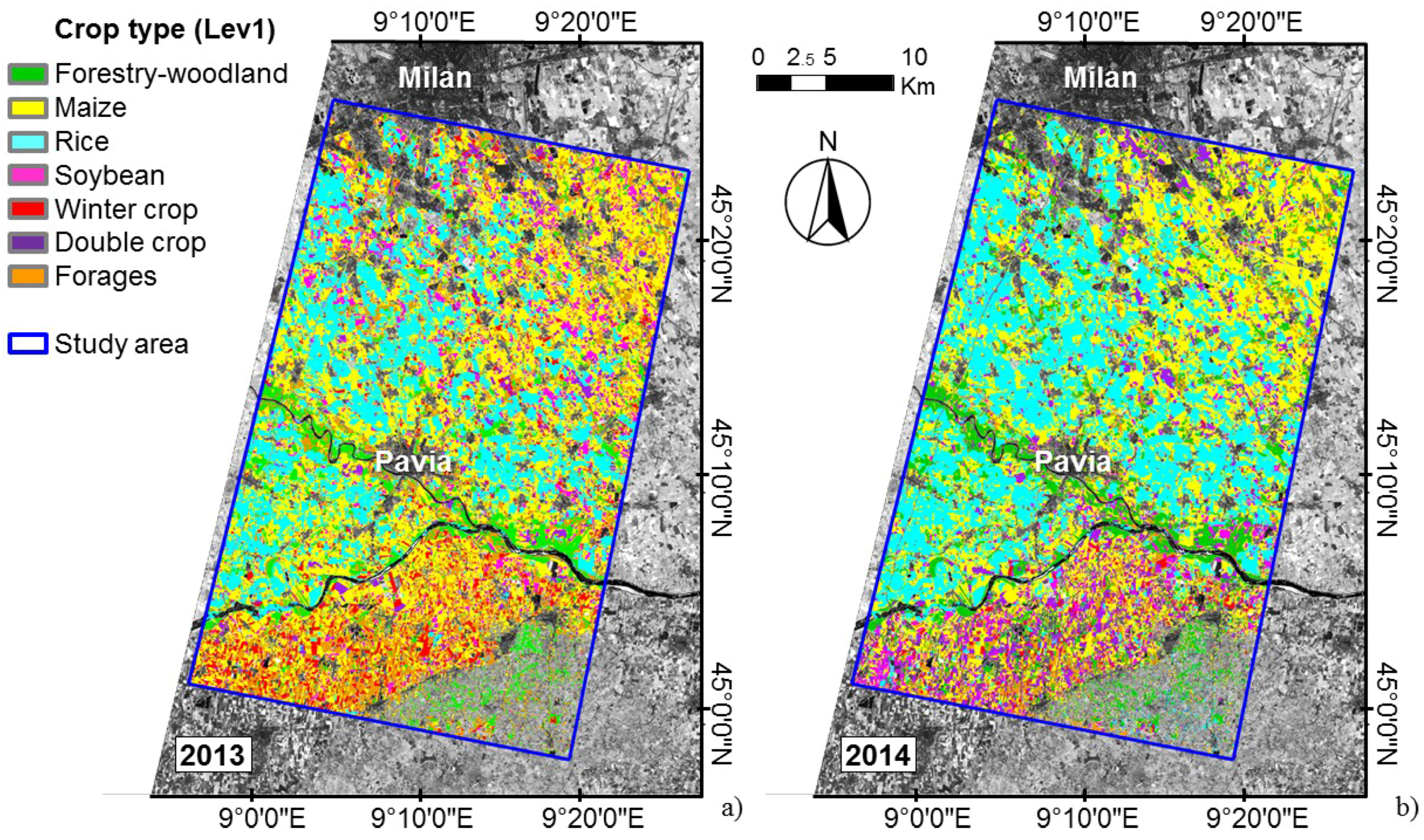
Figure 7. Early in-season crop maps produced using the CTmin-max-ave(ERN+s) scheme over the study area, for the year 2013 (a) and 2014 (b). Crop maps are overlaid on mid-July EVI (16 July 2013 for panel a, 19 July 2014 for panel b), represented in grey tones.
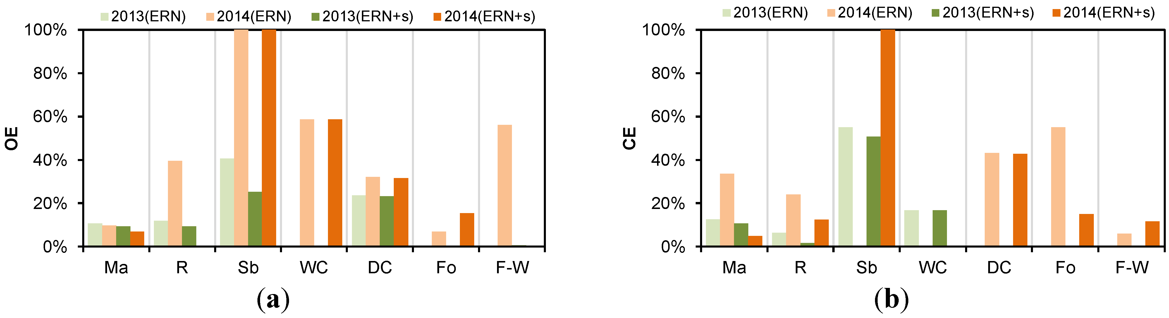
Remotesensing 07 12859 g007
Figure 8. Class omission (OE) (a) and commission (CE) (b) errors at Lev1 for CTmin-max-ave approach implemented over development (year 2013) and transferability (year 2014) sets using different input features (ERN and ERN+s). Ma = maize; R = rice; Sb = soybean; WC = winter crop; DC = double crop; Fo = forages; F-W = forestry-woodland; ERN = EVI+NDFI+RGRI; ERN = EVI+NDFI+RGRI+σ° = ERN+s.
Remotesensing 07 12859 g008
Per-class errors were analyzed at Lev1, providing some insights into the disaggregation of global accuracy results (Figure 8 and Table 7). Using the 2013 validation dataset (case r), depicted in light and dark green bars of Figure 8 and in the two upper matrices of Table 7, OE and CE are consistently lower than 25% for all classes, with the exception of soybean (OE = 25.3%–40.7%, CE = 50.7%–55.0%, with either ERN or ERN+s input), which is mainly misclassified as maize. For the soybean class, the use of X-band σ° results in a OE reduction of 15.4%, due to less confusion with other summer crops, and in a CE reduction of 4.3%, due to less confusion with rice; a reduction of 4.9% CE for rice is also registered using ERN+s input, while errors over other crop types are stable. The best performances, with class errors not exceeding 10% and balanced between omission and commission, are achieved for maize (OE = 9.3%, CE = 10.6%), rice (OE = 9.3%, CE = 1.6%), forages (OE = 0.1%, CE = 0.5%), and forestry-woodland (OE = 0.6%, CE = 0.1%). Tendencies to overestimation for winter crop (CE = 16.8%) and to underestimation for double crop (OE = 23.7%) are observed, due to mutual confusion between these two classes.
Table 7. Confusion matrices of early in-season crop maps produced using the CT scheme implemented over development (2013) and transferability (2014) sets, with ERN and ERN+s input features. Figures are expressed in hectares [ha]. ERN = EVI+NDFI+RGRI; ERN = EVI+NDFI+RGRI+σ° = ERN+s.
Reference Dataset
MaizeRiceSoybeanWinter cropDouble CropForagesForestry-woodland
Development SetCTmin-max-ave(ERN)2013Maize95.68.614.60.00.50.00.1
Rice4.385.16.20.00.00.00.0
Soybean5.72.329.70.00.00.00.0
Winter crop0.00.00.029.17.70.00.0
Double Crop0.00.00.00.028.30.00.0
Forages0.00.00.00.00.019.10.0
Forestry-woodland0.00.00.00.00.00.047.4
CTmin-max-ave(ERN+s)2013Maize95.88.612.40.00.00.00.1
Rice0.487.44.20.00.00.00.0
Soybean9.50.033.80.00.40.00.0
Winter crop0.00.00.029.17.70.00.0
Double Crop0.00.00.00.028.40.00.0
Forages0.00.00.00.00.019.10.3
Forestry-woodland0.00.00.00.00.00.047.2
Transferability SetCTmin-max-ave(ERN)2014Maize61.026.88.60.02.50.00.1
Rice6.641.030.20.00.00.00.0
Soybean0.00.00.00.00.00.00.0
Winter crop0.00.00.014.60.00.00.0
Double Crop0.00.00.019.927.60.50.0
Forages0.00.00.00.08.924.234.7
Forestry-woodland0.00.00.00.01.40.029.8
CTmin-max-ave(ERN+s)2014Maize62.80.013.30.00.00.00.0
Rice4.867.825.20.00.00.00.1
Soybean0.00.00.30.02.30.00.0
Winter crop0.00.00.014.60.00.00.0
Double Crop0.00.00.019.928.10.50.0
Forages0.00.00.00.05.322.40.1
Forestry-woodland0.00.00.03.43.20.064.4
When the CTmin-max-ave scheme is applied to 2014 data (transferability set) in case r (Figure 8, light and dark orange bars, Table 7, two lower confusion matrices), some different patterns emerge: both CE and OE are greater than 2013 over most of the classes. A remarkable case is represented by soybean, with OE = 100.0%, meaning that this class is not represented in the classified pixels belonging to 2014 validation set. These pixels are mistakenly classified as rice (78%) and maize (22%). Other major discrepancies between 2013 and 2014 per-class accuracy occur for winter crop and double crop classes: for the former, the 2014 crop map is strongly underestimating (OE = 58%), while for the latter the rather conservative 2013 performance (CE = 0%) is not repeated for 2014 (CE > 40%, OE > 30%). The overestimation of winter crop is due to confusion with double crop, while the errors observed for double crop come from misclassification not only with winter crop, but also with forages. This could be due to the timing of 2014 acquisition dates, which less effectively capture the single and double crop dynamics compared to 2013 data. The high OE for forestry-woodland (56%) is instead due to class confusion with forages.
The integration of σ° for the 2014 dataset (ERN+s) results in very small changes of OE for soybean, winter crop and double crop, while it brings an improvement for maize (OE = 7.0%, CE = 4.9%), rice (OE = 0.2%, CE = 12.4%), forages (OE = 14.9%, CE = 20.0%), and forestry-woodland (OE = 0.3%, CE = 11.7%); this is mainly due to the reduced confusion between rice and maize and between forages and forestry-woodland. Still, per-class performances using ERN+s over 2014 are generally worse than for 2013, especially over crop classes more sensitive to the seasonal climatic conditions (e.g., double crop and soybean, usually sown late in summer season in Lombardy and thus prone to meteorological fluctuations). A different behavior is shown by rice, with a slight overestimation of class extent for 2014 dataset (<OE, >CE), compared to 2013 results. In summary, CTmin-max-ave performance using ERN+s input is better than with ERN for most of the crop types at Lev1 and outputs acceptable class accuracies ranging from 62.8% for double crop, to >90% for forestry-woodland (94.0%), rice (93.8%), and maize (94.6%). Important misclassification errors are observed for soybean class across the inter-annual dataset.

4.4. Error Reduction Strategy

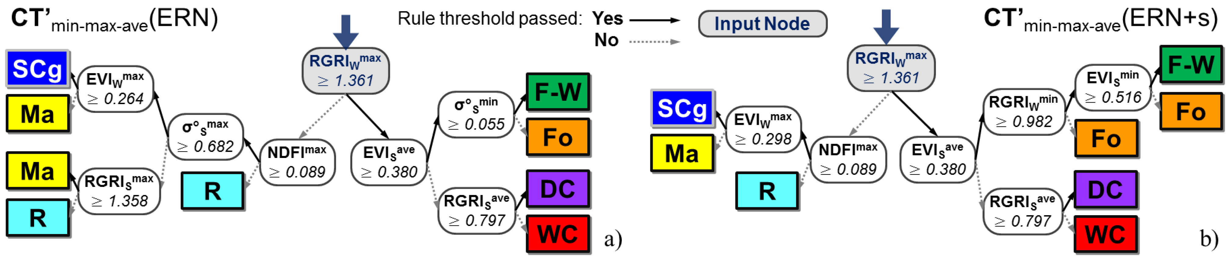
Since Lev1 map assessment showed some misclassification for summer crop classes (especially on 2014 dataset), we tested an expert-based ex-post pruning of the CTmin-max-ave scheme, implemented by restructuring the set of rules for branches with higher class attribution cumulated error (>20%). The rationale is to test the performance of a classifier which reduces the overall classification error at the expenses of the detail of the thematic level. This way, we generate a crop map which is only partially at Lev1 detail (see Table 7 for Lev1 areal coverage percentage), by grouping summer crops, which are in the left branches of the schemes shown in Figure 6 together into a generic crop type label (generic summer crop, SCg) (Figure 9). These re-structured crop mapping schemes, implemented for both ERN and ERN+s are respectively named: CT’min-max-ave(ERN), shown in Figure 9a, and CT’min-max-ave(ERN+s) scheme, shown in Figure 9b.
Validation was carried out using the same validation sets used for assessing CTmin-max-ave results, by excluding the areas labelled as SCg, which are classified now at Lev0. As a consequence, CT’min-max-ave early crop maps do not cover the whole study area at Lev1 and some of the cropland is mapped at Lev0. Table 8 summarizes accuracy metrics of the CT’min-max-ave scheme calculated for two validation datasets: case t and case r. The Lev1 classified coverage ranges from a minimum of 84% (obtained for the ERN 2013 map), to a maximum of 94% of the total study site cropland area (for the ERN 2014 map). As expected, the global accuracy scores achieved with the ex-post pruned schemes are higher than the ones derived with the original CTmin-max-ave schemes: OA (κ) increases by 4.6–4.7% (0.047–0.062) for the year 2013 and by 3.7% (0.051–0.053) for the year 2014. As observed for the original scheme, the best performance for CT’min-max-ave is still achieved over the development set (2013), with OA~95% (κ~0.94). For the transferability set (2014), OA decreases to 70.6% using ERN input, but still a strong rebound of +19.7% (up to 90.3%) is achieved by adding X-band σ° (ERN+s set), with κ increasing from 0.625 to 0.877; the positive contribution of CSK based information for 2014 dataset is thus confirmed.
Figure 9. CT’min-max-ave classification tree schemes for: (a) ERN, and (b) ERN+s input dataset. Ma = maize; R = rice; SCg = summer crop (generic); WC = winter crop; DC = double crop; Fo = forages; F-W = forestry-woodland.
Remotesensing 07 12859 g009
Table 8. Accuracy performance at Lev1 assessed using the CT’min-max-ave scheme (excluding the generic summer crop class), with either ERN or ERN+s input dataset, expressed in terms of OA and κ. The cropland area percentage classified at Lev1 is included. case r = validation set with class distribution proportional to real case crop acreage percent coverage; case t = validation set with class distribution same as training set; ERN = EVI+NDFI+RGRI; ERN = EVI+NDFI+RGRI+σ° = ERN+s.
Validation SetInput Features
2013 Dataset2014 Dataset
ERNERN+sERNERN+s
OAcase t95.0%95.5%--
case r94.8%95.4%70.6%90.3%
κcase t0.9390.945--
case r0.9370.9440.6250.877
Lev1 coverage 88%84%94%90%
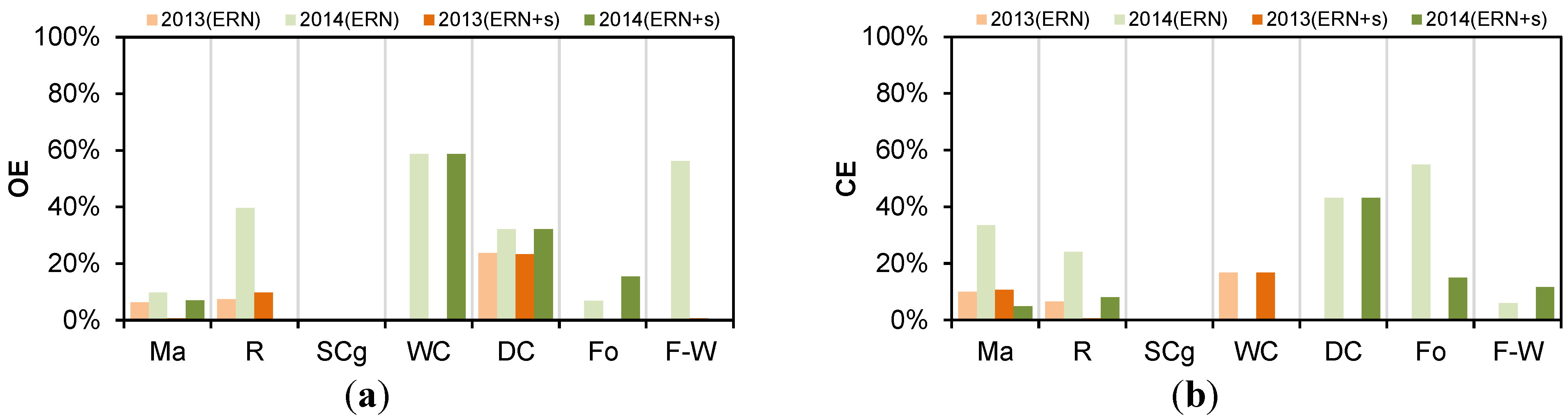
Per-class error analysis (Figure 10) shows that the re-structured schemes provide an improvement only to CE of the summer crop classes, maize and rice (being soybean excluded as target here) with a significant reduction for rice CE (4.4%) over 2014 using ERN+s input set. In summary, the CT’min-max-ave showed slight but consistently better performance of the original scheme, and could be adopted as error reduction strategy when the proposed crop mapping approach is applied to different conditions; this would lead to a crop map with different thematic levels: Lev1, i.e., distinguishing the majority of rice and maize fields , and Lev0.
Figure 10. Class error at Lev1 for the CT’min-max-ave scheme over development (2013) and transferability (2014) sets, using different input features (ERN and ERN+s): (a) OE, (b) CE. Ma = maize; R = rice; SCg = summer crop (generic); WC = winter crop; DC = double crop; Fo = forages; F-W = forestry-woodland; ERN = EVI+NDFI+RGRI; ERN = EVI+NDFI+RGRI+σ° = ERN+s.
Remotesensing 07 12859 g010

5. Conclusions

This study describes a classification tree approach for in-season crop mapping over Northern Italy during the early summer season (mid-July) from the integration of optical (Landsat 8 OLI) and X-band SAR (COSMO-SkyMed) synoptic seasonal features. A rule-based approach offers the advantage of being interpretable through rules/conditions applied to input features, which are representative of crop conditions and development. Results described could be applied to Northern Italy and, with minimal check and tuning by local experts, also to areas with similar environmental and agricultural characteristics (i.e., European temperate to Mediterranean areas).
Key findings and conclusions relevant for crop mapping applications are listed below:
  • The proposed approach produces early in-season (mid-July) crop type maps at two levels of thematic detail with the greatest accuracy obtained when both optical and SAR features (ERN+s set) are used as input: overall accuracy is 91.8% for the 2013 season and 86.6% for the 2014 season;
  • Best performing input features for effectively distinguishing 7 crop types (maize, rice, soybean, winter crop, double crop, forages, forestry-woodland) can be extracted from synoptic seasonal features calculated for winter and summer crops and derived from two combinations of remote sensing proxies for vegetation and soil conditions: i) EVI, NDFI and RGRI from OLI data (ERN set), and ii) the integration of OLI-derived proxies with CSK backscattering (ERN+s set).
  • The contribution of X-band σ° (HH polarization) is relevant for promoting the transferability of the approach over a season (2014) different from the one used for developing the classification rules, with an increment of 19.7% in OA compared to crop maps produced using only optical input features;
  • The integration of CSK σ° reduces class errors (omission and commission) especially for crop types characterized by more seasonally stable agronomic patterns (i.e., maize, rice, forages, forestry-woodland);
  • Expert-based tuning and ex-post pruning are key assets when dealing with operational monitoring and can be used as error reduction strategy, delivering a modified early crop mapping scheme with hybrid thematic level output, and higher overall accuracy (90.3% using ERN+s input for 2014 season);
  • In the framework of agriculture management, the achieved overall accuracy at mid-July is considered satisfactory given the fact that the information on crops is provided early during the growing season as management requires, i.e., 2–3 months before end of season and harvesting;
  • The proposed the approach is interpretable and flexible enough for being exploited for mapping crops at different levels of detail and possibly exploiting different input data with similar spectral bands (e.g., Sentinel-2 MSI).

Supplementary Files

Supplementary File 1

Acknowledgments

The authors thank Mirco Boschetti (CNR-IREA) for the fruitful discussion during the preliminary phase of the work, and Alberto Crema (CNR-IREA) for the support in checking and preparing the crop type reference data. We are grateful to Francesco Holecz and team of Sarmap SA for having provided the software suite MAPscape-RICE used for processing CSK data and for their support in calculating interferometric coherence. Finally, we must thank the academic editor and four anonymous reviewers for their comments and suggestions, which have helped us in enhancing the manuscript.
This work has been conducted in the frame of Space4Agri research project funded and supported by the AQ CNR-Regione Lombardia (CNR, Convenzione Operativa n. 18091/RCC, 05/08/2013). The work was carried out using CSK® Products, © of the Italian Space Agency (ASI), delivered under a license to use by ASI (project title: “Serie temporali di dati Cosmo SkyMed combinate con dati ottici per la mappatura delle varietà e dello stato colture in regione Lombardia”).

Author Contributions

Paolo Villa, Daniela Stroppiana, Giacomo Fontanelli, and Pietro Alessandro Brivio contributed to the experimental design of the study. Paolo Villa, Giacomo Fontanelli, and Ramin Azar run the data preparation and processing. Paolo Villa, Daniela Stroppiana, Giacomo Fontanelli, and Pietro Alessandro Brivio carried out the analysis of results. Paolo Villa and Daniela Stroppiana prepared and wrote the manuscript, and all the authors revised it.

Conflicts of Interest

The authors declare no conflict of interest.

References

  1. Potgieter, A.B.; Lawson, K.; Huete, A.R. Determining crop acreage estimates for specific winter crops using shape attributes from sequential MODIS imagery. Int. J. Appl. Earth Obs. 2013, 23, 254–263. [Google Scholar] [CrossRef]
  2. Hao, P.; Zhan, Y.; Wang, L.; Niu, Z.; Shakir, M. Feature selection of time series MODIS data for early crop classification using Random Forest: A case study in Kansas, USA. Remote Sens. 2015, 7, 5347–5369. [Google Scholar] [CrossRef]
  3. Becker-Reshef, I.; Vermote, E.; Lindeman, M.; Justice, C. A generalized regression-based model for forecasting winter wheat yields in Kansas and Ukraine using MODIS data. Remote Sens. Environ. 2010, 114, 1312–1323. [Google Scholar] [CrossRef]
  4. Rosegrant, M.W.; Cline, S.A. Global food security: challenges and policies. Science 2003, 302, 1917–1919. [Google Scholar] [CrossRef] [PubMed]
  5. Atzberger, C. Advances in remote sensing of agriculture: Context description, existing operational monitoring systems and major information needs. Remote Sens. 2013, 5, 949–981. [Google Scholar] [CrossRef]
  6. Mo, X.; Liu, S.; Lin, Z.; Xu, Y.; Xiang, Y.; McVicar, T.R. Prediction of crop yield, water consumption and water use efficiency with a SVAT-crop growth model using remotely sensed data on the North China Plain. Ecol. Model. 2005, 183, 301–322. [Google Scholar] [CrossRef]
  7. Reichstein, M.; Ciais, P.; Papale, D.; Valentini, R.; Running, S.; Viovy, N.; Cramer, W.; Granier, A.; Ogée, J.; Allard, V.; et al. Reduction of ecosystem productivity and respiration during the European summer 2003 climate anomaly: A joint flux tower, remote sensing and modelling analysis. Glob. Change Biol. 2007, 13, 634–651. [Google Scholar] [CrossRef]
  8. Ozdogan, M.; Yang, Y.; Allez, G.; Cervantes, C. Remote sensing of irrigated agriculture: Opportunities and challenges. Remote Sens. 2010, 2, 2274–2304. [Google Scholar] [CrossRef]
  9. McNairn, H.; Brisco, B. The application of C-band polarimetric SAR for agriculture: A review. Can. J. Remote Sens. 2004, 30, 525–542. [Google Scholar] [CrossRef]
  10. Carlson, R.E.; Aspiazu, C. Cropland acreage estimates from temporal, multispectral ERTS-1 data. Remote Sens. Environ. 1976, 4, 237–243. [Google Scholar] [CrossRef]
  11. Badhwar, G.B. Automatic corn-soybean classification using Landsat MSS data. II. Early season crop proportion estimation. Remote Sens. Environ. 1984, 14, 31–37. [Google Scholar] [CrossRef]
  12. Oetter, D.R.; Cohen, W.B.; Berterretche, M.; Maiersperger, T.K.; Kennedy, R.E. Land cover mapping in an agricultural setting using multiseasonal Thematic Mapper data. Remote Sens. Environ. 2001, 76, 139–155. [Google Scholar] [CrossRef]
  13. Price, K.; Egbert, S.; Lee, R.; Boyce, R.; Nellis, M.D. Mapping land cover in a high plains agroecosystem using a multi-date landsat thematic mapper modeling approach. Trans. Kans. Acad. Sci. 1997, 100, 21–33. [Google Scholar] [CrossRef]
  14. Martínez-Casasnovas, J.A.; Martín-Montero, A.; Casterad, M.A. Mapping multi-year cropping patterns in small irrigation districts from time-series analysis of Landsat TM images. Eur. J. Agron. 2005, 23, 159–169. [Google Scholar] [CrossRef]
  15. Vyas, S.P.; Oza, M.P.; Dadhwal, V.K. Multi-crop separability study of Rabi crops using multi-temporal satellite data. J. Indian Soc. Remote Sens. 2005, 33, 75–79. [Google Scholar] [CrossRef]
  16. Leite, P.B.C.; Feitosa, R.Q.; Formaggio, A.R.; da Costa, G.A.O.P.; Pakzadc, P.; Del’Arco Sanches, L. Hidden Markov Models for crop recognition in remote sensing image sequences. Pattern Recogn. Lett. 2011, 32, 19–26. [Google Scholar] [CrossRef]
  17. Wulder, M.A.; Masek, J.G.; Cohen, W.B.; Loveland, T.R.; Woodcock, C.E. Opening the archive: How free data has enabled the science and monitoring promise of Landsat. Remote Sens. Environ. 2012, 122, 2–10. [Google Scholar] [CrossRef]
  18. Rembold, F.; Maselli, F. Estimation of inter-annual crop area variation by the application of spectral angle mapping to low resolution multitemporal NDVI images. Photogramm. Eng. Remote Sens. 2006, 72, 55–62. [Google Scholar] [CrossRef]
  19. Chang, J.; Hansen, M.C.; Pittman, K.; Carroll, M.; DiMiceli, C. Corn and soybean mapping in the United States using MODIS time-series data sets. Agron. J. 2007, 99, 1654–1664. [Google Scholar] [CrossRef]
  20. An, Q.; Gao, W.; Yang, B.; Wu, Y.; Yu, L.; Liu, Z. Research on feature selection method oriented to crop identification using remote sensing image classification. In Proceedings of the Sixth International Conference on Fuzzy Systems and Knowledge Discovery, Tianjin, China, 14–16 August 2009; Volume 5, pp. 426–432.
  21. Dutta, S.; Sharma, S.A.; Khera, A.P.; Yadav, M.; Hooda, R.S.; Mothikumar, K.E.; Manchanda, M.L. Accuracy assessment in cotton acreage estimation using Indian remote sensing satellite data. ISPRS J. Photogramm. 1994, 49, 21–26. [Google Scholar] [CrossRef]
  22. Dutta, S.; Patel, N.K.; Medhavy, T.T.; Srivastava, S.K.; Mishra, N.; Singh, K.R.P. Wheat crop classification using multidate IRS LISS-I data. J. Indian Soc. Remote Sens. 1998, 26, 7–14. [Google Scholar] [CrossRef]
  23. Aschbacher, J.; Pongsrihadulchai, A.; Karnchanasutham, S.; Rodprom, C.; Paudyal, D.R.; Le Toan, T. Assessment of ERS-1 SAR data for rice crop mapping and monitoring. In Proceedings of the IEEE International Geoscience and Remote Sensing Symposium, Firenze, Italy, 10–14 July 1995; Volume 3, pp. 2183–2185.
  24. Le Toan, T.; Ribbes, F.; Wang, L.-F.; Floury, N.; Kung-Hau, D.; Kong, J.; Fujita, M.; Kurosu, T. Rice crop mapping and monitoring using ERS-1 data based on experiment and modeling results. IEEE Trans. Geosci. Remote Sens. 1997, 35, 41–56. [Google Scholar] [CrossRef]
  25. Dong, Y.; Sun, G.; Pang, Y. Monitoring of rice crop using ENVISAT ASAR data. Sci. China 2006, 49, 755–763. [Google Scholar] [CrossRef]
  26. Wang, X.; Shi, X.; Ling, F. Images difference of ASAR data for rice crop mapping in Fuzhou, China. Geo. Spat. Inf. Sci. 2010, 13, 123–129. [Google Scholar] [CrossRef]
  27. Satalino, G.; Mattia, F.; Le Toan, T.; Rinaldi, M. Wheat crop mapping by using ASAR AP data. IEEE Trans. Geosci. Remote Sens. 2009, 47, 527–530. [Google Scholar] [CrossRef]
  28. Stankiewicz, K.A. The efficiency of crop recognition on ENVISAT ASAR images in two growing seasons. IEEE Trans. Geosci. Remote Sens. 2006, 44, 806–814. [Google Scholar] [CrossRef]
  29. McNairn, H.; Ellis, J.; Van Der Sanden, J.J.; Hirose, T.; Brown, R.J. Providing crop information using RADARSAT-1 and satellite optical imagery. Int. J. Remote Sens. 2002, 23, 851–870. [Google Scholar] [CrossRef]
  30. Moran, M.S.; Vidal, A.; Troufleau, D.; Qi, J.; Clarke, T.R.; Pinter, P.J.; Mitchell, T.A.; Inoue, Y.; Neale, C.M.U. Combining multifrequency microwave and optical data for crop management. Remote Sens. Environ. 1997, 61, 96–109. [Google Scholar] [CrossRef]
  31. Liu, C.; Shang, J.; Vachon, P.W.; McNairn, H. Multiyear crop monitoring using polarimetric RADARSAT-2 data. IEEE Trans. Geosci. Remote Sens. 2013, 51, 2227–2240. [Google Scholar] [CrossRef]
  32. Moran, M.S.; Alonso, L.; Moreno, J.F.; Pilar Cendrero Mateo, M.; de la Cruz, D.F.; Montoro, A. A RADARSAT-2 quad-polarized time series for monitoring crop and soil conditions in Barrax, Spain. IEEE Trans. Geosci. Remote Sens. 2012, 50, 1057–1070. [Google Scholar] [CrossRef]
  33. McNairn, H.; Shang, J.; Jiao, X.; Champagne, C. The contribution of ALOS PALSAR multipolarization and polarimetric data to crop classification. IEEE Trans. Geosci. Remote Sens. 2009, 47, 3981–3992. [Google Scholar] [CrossRef]
  34. Larrañaga, A.; Alvarez-Mozos, J.; Albizua, L. Crop classification in rain-fed and irrigated agricultural areas using Landsat TM and ALOS/PALSAR data. Can. J. Remote Sens. 2011, 37, 157–170. [Google Scholar] [CrossRef]
  35. Bargiel, D.; Herrmann, S. Multi-temporal land-cover classification of agricultural areas in two European regions with high resolution spotlight TerraSAR-X data. Remote Sens. 2011, 3, 859–877. [Google Scholar] [CrossRef]
  36. Balenzano, A.; Satalino, G.; Belmonte, A.; D'Urso, G.; Capodici, F.; Iacobellis, V.; Gioia, A.; Rinaldi, M.; Ruggieri, S.; Mattia, F. On the use of multi-temporal series of COSMO-SkyMed data for land cover classification and surface parameter retrieval over agricultural sites. In Proceedings of the IEEE International Geoscience and Remote Sensing Symposium, Vancouver, Canada, 24–29 July 2011; pp. 142–145.
  37. McNairn, H.; Kross, A.; Lapen, D.; Caves, R.; Shang, J. Early season monitoring of corn and soybeans with TerraSAR-X and RADARSAT-2. Int. J. Appl. Earth Obs. Geoinf. 2014, 28, 252–259. [Google Scholar] [CrossRef]
  38. Satalino, G.; Panciera, R.; Balenzano, A.; Mattia, F.; Walker, J. COSMO-SkyMed multi-temporal data for land cover classification and soil moisture retrieval over an agricultural site in Southern Australia. In Proceedings of the IEEE International Geoscience and Remote Sensing Symposium, Munich, Germany, 22–27 July 2012; pp. 5701–5704.
  39. Sonobe, R.; Tani, H.; Wang, X.; Kobayashi, N.; Shimamura, H. Random forest classification of crop type using multi-temporal TerraSAR-X dual-polarimetric data. Remote Sens. Lett. 2014, 5, 157–164. [Google Scholar] [CrossRef]
  40. Gerstl, S.A.W. Physics concepts of optical and radar reflectance signatures A summary review. Int. J. Remote Sens. 1994, 11, 1109–1117. [Google Scholar] [CrossRef]
  41. Forkuor, G.; Conrad, C.; Thiel, M.; Ullmann, T.; Zoungrana, E. Integration of optical and Synthetic Aperture Radar imagery for improving crop mapping in Northwestern Benin, West Africa. Remote Sens. 2014, 6, 6472–6499. [Google Scholar] [CrossRef]
  42. Pohl, C.; Van Genderen, J.L. Review article multisensor image fusion in remote sensing: Concepts, methods and applications. Int. J. Remote Sens. 1998, 19, 823–854. [Google Scholar] [CrossRef]
  43. Stafford, J.V. Implementing precision agriculture in the 21st century. J. Agric. Eng. Res. 2000, 76, 267–275. [Google Scholar] [CrossRef]
  44. Michelson, D.B.; Liljeberg, B.M.; Pilesjo, P. Comparison of algorithms for classifying Swedish landcover using LANDSAT TM and ERS-1 SAR data. Remote Sens. Environ. 2000, 71, 1–15. [Google Scholar] [CrossRef]
  45. Blaes, X.; Vanhalle, V.; Defourny, P. Efficiency of crop identification based on optical and SAR image time series. Remote Sens. Environ. 2005, 96, 352–365. [Google Scholar] [CrossRef]
  46. McNairn, H.; Champagne, C.; Shang, J.; Holmstrom, D.; Reichert, G. Integration of optical and Synthetic Aperture Radar (SAR) imagery for delivering operational annual crop inventories. ISPRS J. Photogramm. 2009, 64, 434–449. [Google Scholar] [CrossRef]
  47. Skakun, S.; Kussul, N.; Shelestov, A.; Lavreniuk, M.; Kussul, O. Efficiency assessment of multitemporal C-band Radarsat-2 intensity and Landsat-8 surface reflectance satellite imagery for crop classification in Ukraine. IEEE J. Sel. Topics Appl. Earth Obs. Remote Sens. 2015, in press. [Google Scholar] [CrossRef]
  48. De Oliveira Pereira, L.; da Costa Freitas, C.; Sant´ Anna, S.J.S.; Lu, D.; Moran, E.F. Optical and radar data integration for land use and land cover mapping in the Brazilian Amazon. GISci. Remote Sens. 2013, 50, 301–321. [Google Scholar]
  49. Zhu, Z.; Woodcock, C.E.; Rogan, J.; Kellndorfer, J. Assessment of spectral, polarimetric, temporal, and spatial dimensions for urban and peri-urban land cover classification using Landsat and SAR data. Remote Sens. Environ. 2012, 117, 72–82. [Google Scholar] [CrossRef]
  50. Stroppiana, D.; Azar, R.; Calò, F.; Pepe, A.; Imperatore, P.; Boschetti, M.; Silva, J.M.N.; Brivio, P.A.; Lanari, R. Integration of optical and SAR data for burned area mapping in Mediterranean Regions. Remote Sens. 2015, 7, 1320–1345. [Google Scholar] [CrossRef]
  51. Friedl, M.A.; Brodley, C.E. Decision tree classification of land cover from remotely sensed data. Remote Sens. Environ. 1997, 61, 399–409. [Google Scholar] [CrossRef]
  52. Lawrence, R.L.; Wright, A. Rule-based classification systems using classification and regression tree (CART) analysis. Photogramm. Eng. Remote Sens. 2001, 67, 1137–1142. [Google Scholar]
  53. Vieira, M.A.; Formaggio, A.R.; Rennó, C.D.; Atzberger, C.; Aguiar, D.A.; Mello, M.P. Object Based Image Analysis and Data Mining applied to a remotely sensed Landsat time-series to map sugarcane over large areas. Remote Sens. Environ. 2012, 123, 553–562. [Google Scholar] [CrossRef]
  54. Azar, R.; Villa, P.; Stroppiana, D.; Crema, A.; Boschetti, M.; Brivio, P.A. Multi-temporal assessment of crop classification performance using Landsat 8 OLI data: A test case in Northern Italy. Int. J. Remote Sens. 2015. submited. [Google Scholar]
  55. Odenweller, J.B.; Johnson, K.I. Crop identification using Landsat temporal-spectral profiles. Remote Sens. Environ. 1984, 14, 39–54. [Google Scholar] [CrossRef]
  56. Murthy, C.S.; Raju, P.V.; Badrinath, K.V.S. Classification of wheat crop with multi-temporal images: Performance of maximum likelihood and artificial neural networks. Int. J. Remote Sens. 2003, 24, 4871–4890. [Google Scholar] [CrossRef]
  57. Wardlow, B.D.; Egbert, S.L. Large-area crop mapping using time-series MODIS 250 m NDVI data: An assessment for the US Central Great Plains. Remote Sens. Environ. 2008, 112, 1096–1116. [Google Scholar] [CrossRef]
  58. Foerster, S.; Kaden, K.; Foerster, M.; Itzerott, S. Crop type mapping using spectral–temporal profiles and phenological information. Comput. Electron. Agric. 2012, 89, 30–40. [Google Scholar] [CrossRef]
  59. Asilo, S.; de Bie, K.; Skidmore, A.; Nelson, A.; Barbieri, M.; Maunahan, A. Complementarity of two rice mapping approaches: Characterizing strata mapped by hypertemporal MODIS and rice paddy identification using multitemporal SAR. Remote Sens. 2014, 6, 12789–12814. [Google Scholar] [CrossRef]
  60. Nelson, A.; Setiyono, T.; Rala, A.B.; Quicho, E.D.; Raviz, J.V.; Abonete, P.J.; Maunahan, A.A.; Garcia, C.A.; Bhatti, H.Z.M.; Villano, L.S.; et al. Towards an operational SAR-based rice monitoring system in Asia: Examples from 13 demonstration sites across Asia in the RIICE project. Remote Sens. 2014, 6, 10773–10812. [Google Scholar] [CrossRef]
  61. Giuca, S.; Giannini, M.S.; Nebuloni, A.; Pretolani, R.; Pieri, R.; Cagliero, R.; Marras, F.; Gay, G. Lombardy Agriculture in Figures—2013; INEA: Milan, Italy, 2014; Available online: http://dspace.inea.it/bitstream/inea/846/1/Lombardy_agric_figures_2013.pdf (accessed on 15 May 2015).
  62. ERSAF, Regione Lombardia. Carta dell’utilizzo agricolo annuale. Available online: http://www.ersaf.lombardia.it/servizi/Menu/dinamica.aspx?idArea=16914&idCat=17255&ID=22103 (accessed on 13 July 2015).
  63. Barsi, J.A.; Lee, K.; Kvaran, G.; Markham, B.L.; Pedelty, J.A. The spectral response of the Landsat-8 operational land imager. Remote Sens. 2014, 6, 10232–10251. [Google Scholar] [CrossRef]
  64. Richter, R.; Schläpfer, D. Atmospheric/Topographic Correction for Satellite Imagery; DLR report DLR-IB 565-01/13; ReSe Applications: Wil, Switzerland, 2014; Available online: http://atcor.com/pdf/atcor3_manual.pdf (accessed on 18 May 2015).
  65. Huete, A.R.; Liu, H.Q.; Batchily, K.; Van Leeuwen, W.J.D.A. A comparison of vegetation indices over a global set of TM images for EOS-MODIS. Remote Sens. Environ. 1997, 59, 440–451. [Google Scholar] [CrossRef]
  66. Huete, A.; Didan, K.; Miura, T.; Rodriguez, E.P.; Gao, X.; Ferreira, L.G. Overview of the radiometric and biophysical performance of the MODIS vegetation indices. Remote Sens. Environ. 2002, 83, 195–213. [Google Scholar] [CrossRef]
  67. Boschetti, M.; Nutini, F.; Manfron, G.; Brivio, P.A.; Nelson, A. Comparative analysis of normalised difference spectral indices derived from MODIS for detecting surface water in flooded rice cropping systems. PloS ONE 2014, 9. [Google Scholar] [CrossRef] [PubMed]
  68. Gamon, J.A.; Surfus, J.S. Assessing leaf pigment content and activity with a reflectometer. New Phytol. 1999, 143, 105–117. [Google Scholar] [CrossRef]
  69. Fontanelli, G.; Crema, A.; Azar, R.; Stroppiana, D.; Villa, P.; Boschetti, M. Agricultural crop mapping using optical and SAR multi-temporal seasonal data: A case study in Lombardy region, Italy. In Proceedings of the IEEE International Geoscience and Remote Sensing Symposium, Quebec city, Canada, 13–18 July 2014; pp. 1489–1492.
  70. Holecz, F.; Collivignarelli, F.; Barbieri, M. Estimation of cultivated area in small plot agriculture in Africa for food security purposes. In Proceedings of the ESA Living Planet Symposium, Edinburgh, UK, 9–13 September 2013.
  71. Srivastava, H.S.; Patel, P.; Navalgund, R.R. Application potentials of synthetic aperture radar interferometry for land-cover mapping and crop-height estimation. Curr. Sci. India 2006, 91, 783–788. [Google Scholar]
  72. De Grandi, G.F.; Leysen, M.; Lee, J.S.; Schuler, D. Radar reflectivity estimation using multiple SAR scenes of the same target: technique and applications. In Proceedings of the IEEE International Geoscience and Remote Sensing Symposium, Singapore, 3–8 August 1997; Volume 2, pp. 1047–1050.
  73. Vijaya, V.; Niveditha, G.J. Classification of COSMO SkyMed SAR data based on coherence and backscattering coefficient. Int. J. Comput. Sci. Inf. 2012, 1, 60–63. [Google Scholar]
  74. Witten, I.H.; Frank, E. Data Mining: Practical Machine Learning Tools and Techniques, 2nd ed.; Morgan Kaufmann: San Francisco, CA, USA, 2005; pp. 373–379. [Google Scholar]
  75. Quinlan, J.R. Improved Use of Continuous Attributes in C4.5. J. Artif. Intell. Res. 1996, 4, 77–90. [Google Scholar]
  76. Ruggieri, S. Efficient C4.5. IEEE Trans. Knowl. Data Eng. 2002, 14, 438–444. [Google Scholar] [CrossRef]
  77. Congalton, R.G. A review of assessing the accuracy of classifications of remotely sensed data. Remote Sens. Environ. 1991, 37, 35–46. [Google Scholar] [CrossRef]
  78. Breiman, L. Random Forests. Mach. Learn. 2001, 45, 5–32. [Google Scholar] [CrossRef]
  79. Chan, J.C.W.; Paelinckx, D. Evaluation of Random Forest and Adaboost tree-based ensemble classification and spectral band selection for ecotope mapping using airborne hyperspectral imagery. Remote Sens. Environ. 2008, 112, 2999–3011. [Google Scholar] [CrossRef]
  80. Gislason, P.O.; Benediktsson, J.A.; Sveinsson, J.R. Random Forests for land cover classification. Pattern Recogn. Lett. 2006, 27, 294–300. [Google Scholar] [CrossRef]
  81. Pal, M. Random Forest classifier for remote sensing classification. Int. J. Remote Sens. 2005, 26, 217–222. [Google Scholar] [CrossRef]
  82. Richards, J.A.; Jia, X. Remote Sensing Digital Image Analysis: An Introduction, 3rd ed.; Springer-Verlag: Berlin, Germany, 1999. [Google Scholar]
  83. Swain, P.H.; King, R.C. Two Effective Feature Selection Criteria for Multispectral Remote Sensing. In Proceedings of the 1st International Joint Conference on Pattern Recognition, Washington, DC, USA, 30 October–1 November 1973; pp. 536–540.

