Assessing Optimal Flight Parameters for Generating Accurate Multispectral Orthomosaicks by UAV to Support Site-Specific Crop Management

Abstract

This article describes the technical specifications and configuration of a multirotor unmanned aerial vehicle (UAV) to acquire remote images using a six-band multispectral sensor. Several flight missions were programmed as follows: three flight altitudes (60, 80 and 100 m), two flight modes (stop and cruising modes) and two ground control point (GCP) settings were considered to analyze the influence of these parameters on the spatial resolution and spectral discrimination of multispectral orthomosaicked images obtained using Pix4Dmapper. Moreover, it is also necessary to consider the area to be covered or the flight duration according to any flight mission programmed. The effect of the combination of all these parameters on the spatial resolution and spectral discrimination of the orthomosaicks is presented. Spectral discrimination has been evaluated for a specific agronomical purpose: to use the UAV remote images for the detection of bare soil and vegetation (crop and weeds) for in-season site-specific weed management. These results show that a balance between spatial resolution and spectral discrimination is needed to optimize the mission planning and image processing to achieve every agronomic objective. In this way, users do not have to sacrifice flying at low altitudes to cover the whole area of interest completely.

1. Introduction

Precision agriculture (PA) can be defined as the art and science of using advanced technology to enhance crop production [1]. PA involves better management of farm inputs such as fertilizer, fuel, seed, irrigation, and pesticides, among others, by doing the right management practice at the right place and the right time [2]. PA based on a previous map of any of the variables of interest can be performed by using remote sensing (RS) technology. RS in agriculture is based on the measurement of electromagnetic radiation from soil or plants by sensors on-board satellites and aerial platforms. RS can be used in a wide range of applications and studies such as on crop nutrients [3], infestations of weeds [4], soil properties [5,6], rangelands environments [7], among others. Early Site-Specific Weed Management (ESSWM) involves four steps: (i) weed monitoring, consisting of the detection of weeds; (ii) decision-making; (iii) precision field operation; and (iv) evaluation of the economic profitability, safety and environmental impact of the field operations for the next season [8]. To monitor and detect weeds, it is useful to produce prescription maps, obtained from analysis of remote images captured of the field crop. These images have usually been registered by sensors on board of two traditional platforms, satellite and manned aircraft. However, the evolution of PA demands very high spatial and temporal resolution, measuring even the characteristics of individual plants in some applications. These traditional platforms present problems related to temporal and spatial resolution, and the successful use of these platforms is dependent on weather conditions. Currently, unmanned aerial vehicles (UAVs) are an alternative to acquire remote images at the right moment and repeatedly, making possible the combination of high spatial, spectral and temporal resolutions [9,10].

In most weed control strategies, it is necessary to monitor and detect the weeds at an early growth stage of the crop to avoid the strong competition between weeds and crop in the early phases. The spatial distribution of weeds within crops consist of small patches, which suggests the use of very high spatial resolution imagery [8]. Recent studies on crop-weed discrimination using UAV are based on two steps: (i) to distinguish bare soil and vegetation (crop and weeds) and (ii) to define the crop line to then discriminate crop and weeds [11]. The combination of flight parameters and types of sensors is critical to obtain an adequate spatial resolution and spectral discrimination on the geomatic products for application to weed detection. Spatial resolution, flight parameters and photogrammetric processing of remote images acquired by metric sensors are considered classic photogrammetry and have been well studied and documented [12,13]. In addition, the influence of GPS applications in aerial-triangulation and the accuracy of GPS blocks for various cases of overlap and numbers of GCPs [14], accuracy assessment of digital elevation models [15] and other studies have contributed to the definition of a standardized processing framework. This facilitated the government development of technical specifications for orthophoto production to ensure the quality of spatial and spectral results [16]. However, data acquisition by UAV platforms for research applications is still at an early stage [17,18]. One of the consequences of this early stage of development is that the operational framework for working with UAV platforms is not defined in some aspects. For traditional platforms, parameters such as altitude Above Ground Level (AGL), mode of flight or number of GCPs, among others, determine the spatial and spectral quality of the orthomosaicked images produced. Moreover, these parameters are dependent on UAV architecture (e.g., rotor-wing, fixed-wing, kite) and the type of sensor used.

Altitude AGL defines the pixel size of registered images, area flown over and the flight duration. Therefore, it is necessary to know the pixel size required to achieve a specific objective [19]. Hengl (2006) [20] has established that, in general, at least four pixels are required to detect the smallest object in an image. Therefore, the selection of altitude AGL has to guarantee a sufficiently fine spatial resolution and spectral discrimination and to cover as much surface as possible to optimize the UAV flight [21]. Regarding the mode of flight using a multi-rotor UAV, it is possible to acquire images considering three modes: (1) manual; (2) stop; and (3) cruising mode [22]. The first mode (manual) is used when no flight planning is available, while stop and cruising modes require planning. Both stop mode [23] and cruising mode [21] have been used for multi-rotor UAV. However, flying in cruising mode has a substantial impact on the use of these types of UAV because cruising mode can reduce the flight time required by 75% [24]. Finally, referring to GCPs and considering traditional piloted platforms, the distribution and number of GCPs affect the spatial accuracy of ortho-rectified images [25]. This influence has not been studied and standardized, and therefore, the number of GCPs covers a broad range, from just 4 GCPs [26] to 20 GCPs [27] or even 130 GCPs [17].

Considering spectral discrimination, remote sensing imagery is usually based on the wavelength reflectance of particular leaves and canopies in the visible range of the spectrum (red, green, blue, RGB) and non-visible as near-infrared (NIR) and on the emission of far-infrared (thermal). Reflectance is measured using visible [28], multispectral [29], hyper-spectral [30] and thermal sensors [31]. Multispectral sensors capture narrow wavelength bands to support defining the spatial variability of conditions, for example, weed infestation, that affect crop production or determining the most effective management strategy. These sensors can have single or multiple objectives. Single objective sensors acquire data in three bands that cover the visible region (RGB). It is possible to adapt single objective sensors to operate over a portion of the visible region and infrared (e.g., red, blue, infrared: RBNIR, or red, green, infrared: RGNIR), but the single objective sensors are not able to capture information in both regions (RGB-NIR) at the same time. RGB sensors have been used to determine the spatial quality of orthomosaicks [32] or vegetation fraction mapping by calculating different visible spectral indices to discriminate vegetation in wheat fields early in the season [33]. GB-NIR customized sensors can also be used for crop monitoring by calculating a green normalized difference vegetation index to support site-specific agricultural decision making [34]. These single objective sensors are low in weight and compact in size, making them interesting for use in UAV and several agricultural approaches. However, the single sensor does not cover the full region of interest (RGB-NIR) at the same time, reducing the possibilities of its use. Currently, the sensor that covers this region of interest is a multispectral sensor equipped with multiple arrays of sensors. Each band corresponds to a specific sensor, and the specific sensors are higher quality sensors [7]. A multiple array sensor can increase the number and type of vegetation indices to be calculated, being more polyvalent for use in PA. These types of sensors are heavier than a single objective sensor, impacting the UAV flight programming negatively. Huang et al. (2010) [35] reported that the multispectral sensors have a slow imaging speed that limits their application. Furthermore, multi-objective sensors work with an individual sensor per band at the same time (normally, 4, 6 or 12), working with more than one sensor simultaneously. All these aspects highlight that it is necessary to define a framework to optimize multi-array spectral sensor flights.

To our knowledge, no detailed investigation has been conducted regarding the influence of UAV flight parameters such as altitude AGL, mode of flight and number and distribution of GCPs on the spatial resolution and spectral discrimination of multispectral orthomosaicks using a multi-array sensor on-board a multi-rotor UAV. This paper defines the best technical specifications for working with a multispectral sensor on-board a multi-rotor UAV to obtain the most accurate spatial and spectral orthophoto to be used in precision agriculture tasks.

2. Material and Methods

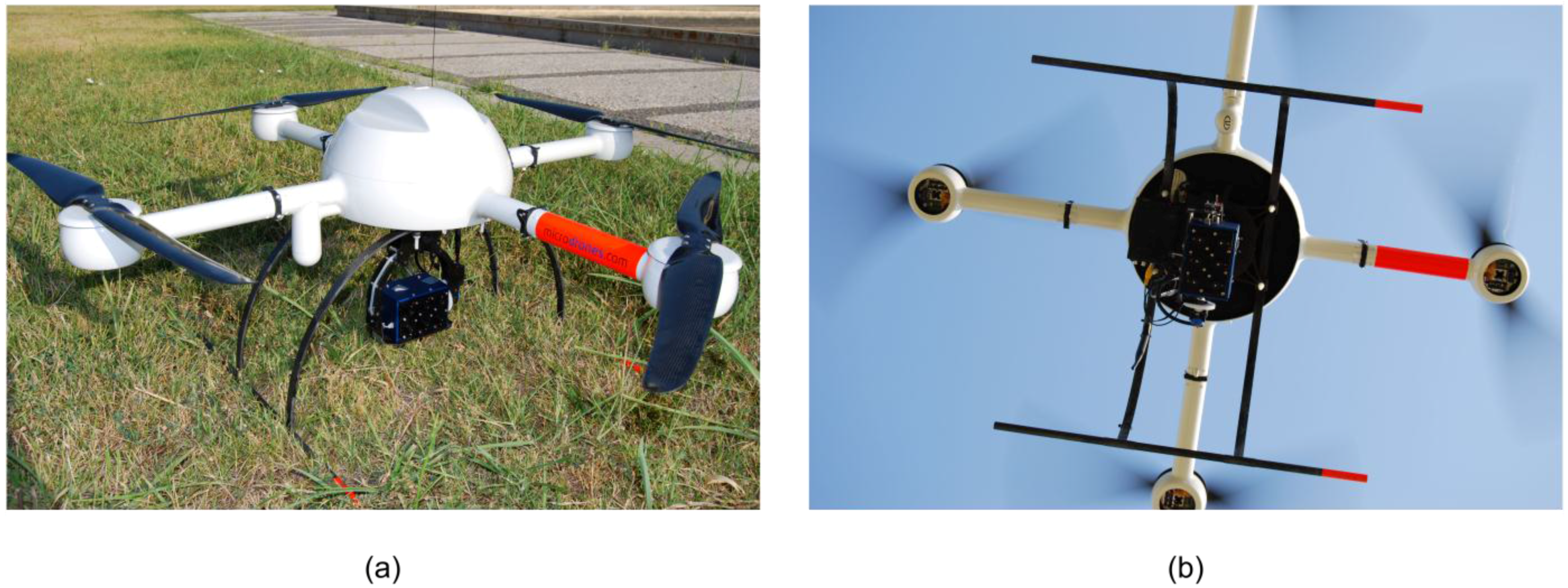
2.1. UAV and Sensor Description

A quadrocopter, model MD4-1000 (Microdrones GmbH, Siegen, Germany), was used as UAV to perform all flights. It is a vertical take-off and landing aircraft. This platform is entirely carbon design and it is equipped with 4 × 250W gearless brushless motors powered by a 22.2 V battery. The maximum cruising speed is 12.0 m/s and maximum climb speed 7.5 m/s. MD4-1000 can fly by remote control or automatically. Flight radius considering remote control by radio is 500 meters. Remote control is used to start the UAV’s engines, manage take-off and landing, complete flight in manual mode and start autonomous navigation. The maximum payload mass is 1.2 kg, being a recommended payload mass equal to 0.8 kg. This system can operate from a few meters to a ceiling altitude of 1000 m. MD4-1000 UAV can carry any lightweight sensor mounted in its gimbal. Flying time is function of sensor weight and windy conditions. Considering sensor weight, the range is from 30 to 20 minutes for 250-g to 700-g respectively.

As payload we used a TetraCam mini-MCA6 (TetraCam Inc., Chatsworth, CA, USA) (Figure 1a). It is a lightweight multispectral rolling shutter camera, 700-g, with six individual sensors, one for each band, arranged in a 2 × 3 array. Each sensor has a focal length equals to 9.6 mm and a 1.3-megapixel (1280 × 1024 pixels) CMOS sensor that stores images on a compact flash card. One of the sensors plays as master channel and the other five as “slaves”. Master channel is used as reference channel. It calculates its own exposure time, defining global settings used for slave sensors to ensure the simultaneity of images acquisition by all of the channels. The camera can store images with 8-bit or 10-bit radiometric resolution, the latter being used in the camera settings. The camera has user-configurable band-pass filters (Andover Corporation, Salem, NH, USA) with a 10-nm full width at half-maximum and center wavelengths of 450 nm (blue region of the electromagnetic spectrum), 530 nm (green region), 670 and 700 nm (red region), 740 nm (red-edge region) and 780 nm (near-infrared region). These bandwidth filters were selected across the visible and NIR regions with regard to well-known biophysical indices developed for vegetation monitoring as described in Kelecey and Lucieer (2012) [36]. During the flight the sensor acquires vertical images (Figure 1b). The image triggering is activated by an MD4-1000 autopilot considering flight settings. For each shoot, the UAV autopilot sends a signal to the sensor to register an image and simultaneously records the GPS location, navigation angles (yaw, roll and pitch) and timestamp on an SD-Card. This information will be used as the initial values in photogrammetric processing. Individual images were pre-processed by PixelWrench2 [37]. Pre-processing consisted of the correct vignette effect, alignment of raw images and generation of multi-band TIFs as explained in [19].

Figure 1. Details of TetraCam mini-MCA6: (a) before takeoff and (b) during flight.

Figure 1. Details of TetraCam mini-MCA6: (a) before takeoff and (b) during flight.

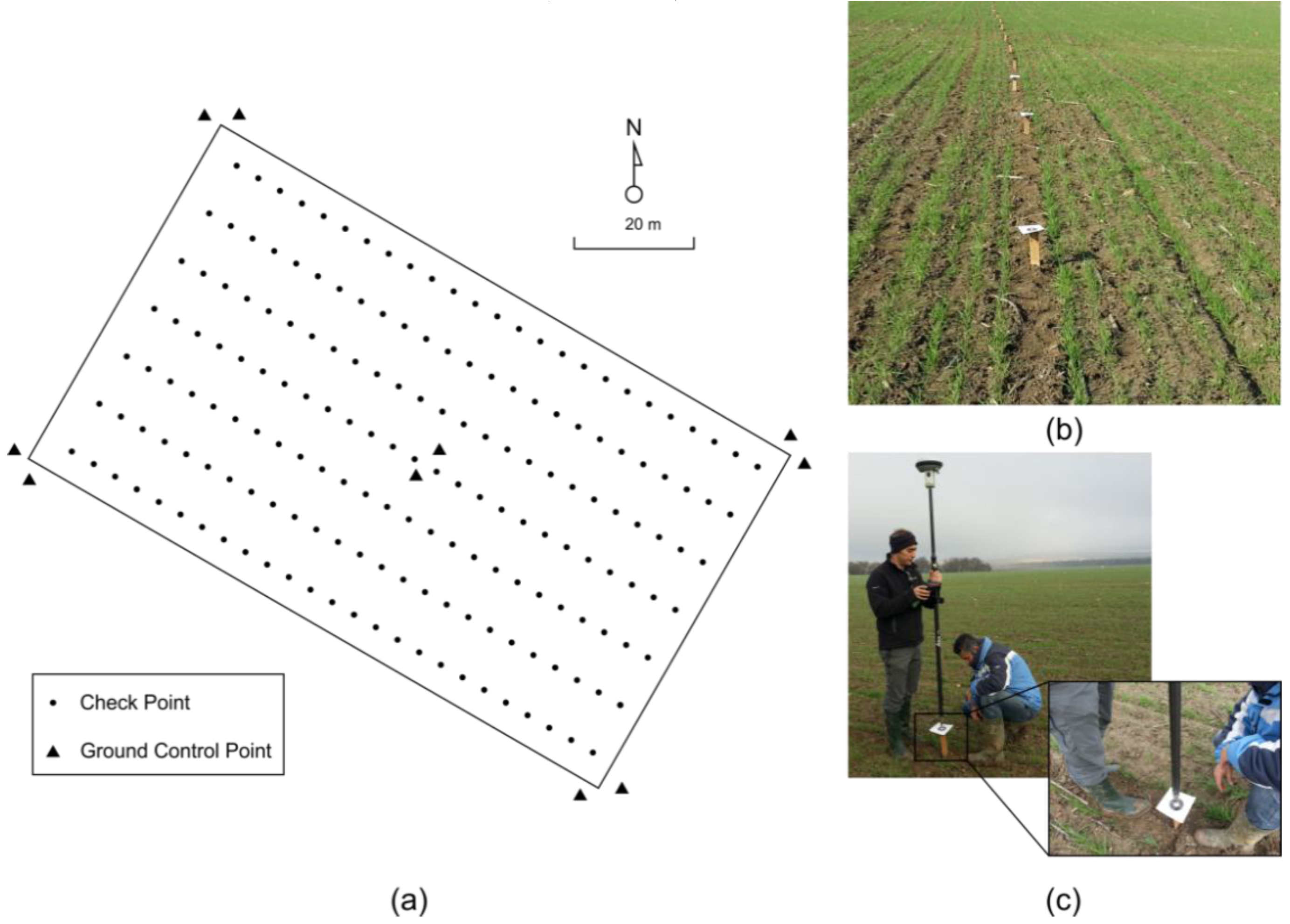
2.2. Study Site and UAV Flights

The study was conducted in a wheat field located in Córdoba (southern Spain) approximately 1.12 ha (80 × 140 m) in size. The ground is flat, with a slope of less than 1%. The wheat crop was sown on 22 November 2014, at 160 kg ha-1 in rows 0.17 m apart, and emergence of the wheat plants started by 15 days after sowing. The field was naturally infested with the broadleaved weed Sinapis arvensis L. (mustard). Wheat crop plants were in the principal stage 2 (tillering), and weed plants were in the principal stage 1 (leaf development, four-six true leaves, codes 14–16) of the BBCH (Biologische Bundesanstalt, Bundessortenamt und CHemische Industrie) extended scale [38]. Different flight missions were planned, considering sensor and UAV specifications. Flight parameters and their formulas have been widely described, for example, [39]. One of the most important flight parameters is altitude AGL, and three different altitudes were considered: 60, 80 and 100 m. Each altitude AGL showed the following different Ground Sample Distance (GSD) values: 3-, 4- and 5-cm×pixel⁻¹, respectively. All the flights were conducted with an 80% forward-lap and a 50% side-lap. Finally, two acquisition imagery modes were considered: stop mode and cruising mode. In stop mode, the UAV vehicle was programmed to fly to each predefined waypoint and to stop at this position. The UAV vehicle hovered over this position during a small interval of time or until positional accuracy was satisfying. In this mode, flight speed was 5 m×s⁻¹ between waypoints. In cruising mode, images were taken when the UAV vehicle was flying and not stopped for image acquisition. Because both flight modes must have the same flight settings, we set up the flight speed and intervals between images to keep the forward-lap and side-lap equal to 80% and 50%, respectively. For an altitude AGL of 60 m, the flight speed was equal to 2 m×s⁻¹, while for 80 and 100 m, the flight speed was 3 m×s⁻¹. The photo interval for all altitudes AGL was 3 s.

Subsequently, each UAV flight was processed considering two different GCP settings (Figure 2a): (i) four GCPs (4 GCPs) and (ii) five GCPs (5 GCPs). These GCPs were used in the aerial triangulation phase to locate the photogrammetric block into a coordinate system. Referring to the 4 GCPs setting, a total of eight GCPs were located on the corners of the study area, two for each corner. The 5 GCPs setting used the same points as the previous configuration and, in addition, two more GCPs in the center of the area. Each GCP was measured with the Stop and Go technique as relative positioning by means of the NTRIP protocol (The Radio Technical Commission for Maritime Services, RTCM, for Networked Transfer via Internet Protocol) using two GNSS receivers: one of the receivers was a reference station from the GNSS RAP network from the Institute for Statistics and Cartography of Andalusia, Spain, and the other, Leica GS15 GNSS, was a rover receiver.

2.3. Photogrammetric Processing

Tetracam mini-MCA6 registers six individual images, one for each individual sensor. Therefore, an alignment process is needed to group individual images taken with each shutter. The alignment was made using Tetracam PixelWrench 2 (PW2) software (Tetracam Inc., Chatsworth, CA, USA). This solution uses a calibration file that contains information about the relative position (translation, rotation and scaling) between master channel and slave channels.

The photogrammetric processing was performed using Pix4Dmapper (Pix4D S.A., Lausanne, Switzerland). Pix4Dmapper is divided into 4 phases: (1) aerial triangulation; (2) Digital Surface Model (DSM) generation; (3) rectification of individual images, and, finally; (4) orthomosaick. All processes are automated except the measurement of GCPs. This automation is based on the use of fundamental principles of Photogrammetry combined with robust algorithms from computer vision [40,41].Aerial triangulation consists of determining the individual orientation of each stereo model of a photogrammetric block. One of the most commonly used and most rigorous methods is the bundle adjustment, which permits the absolute orientation of an entire block of an unlimited number of images using a few GCPs [42]. To perform the bundle adjustment, algorithms are based on “structure from motion”(SfM) techniques. SfM techniques are tolerant of change in view point and can identify and reject the errors when they occur [40,43]. The first stage of an SfM process is to extract features in individual images that can be matched to their corresponding features in other images from the UAV flight. These matched points are used to establish relative locations of the sensors during the flight and to simultaneously calculate the sensor parameters of each image. The whole process is calculated using an incremental approach in which bundle adjustment of an initial image pair is sequentially repeated, with more images incorporated at each iteration [44]. The aerial triangulation for each individual sensor is processes simultaneously taking into account its own specific lens distortion. The result of this phase is the determination of position and orientation for each individual sensor location. With these data, a reconstruction of the surface was produced by a dense point cloud using multi-view stereo matching [45,46]. A DSM was generated using a grid interpolation of the dense point cloud from each individual sensor. Every single image was ortho-rectified using the external orientation and the DSM. Finally, individual ortho-rectified images were combined into a seamless 6-band multispectral orthomosaicked image to obtain the UAV orthophoto of the entire area of interest. Because each spectral band has been processed taking into account their own characteristics and the spatial relation with the others, the band to band alignment is reached.

Two types of orthomosaicked imagery were produced to assess their spatial resolution and spectral discrimination. Referring to spatial resolution, all the UAV flights were processed to generate orthomosaicked images with a unique GSD value equal to 5 cm. This GSD corresponds to the highest GSD value that was obtained in flight (100 m AGL). This degradation of spatial resolution was performed to obtain pixel resolutions of 5 cm in any of the orthomosaicked images independent of the flight altitude, aimed at the objective of studying the effects of UAV flight parameters on spatial resolution. Then, to also assess the quality of the spectral discrimination, the best setting, referring to flight mode and the number and distribution of GCPs was considered. In this context, three orthomosaicked images with a GSD equal to the GSD corresponding to each flight (i.e., GSD ranging from 3- to 5- cm×pixel⁻¹) were produced.

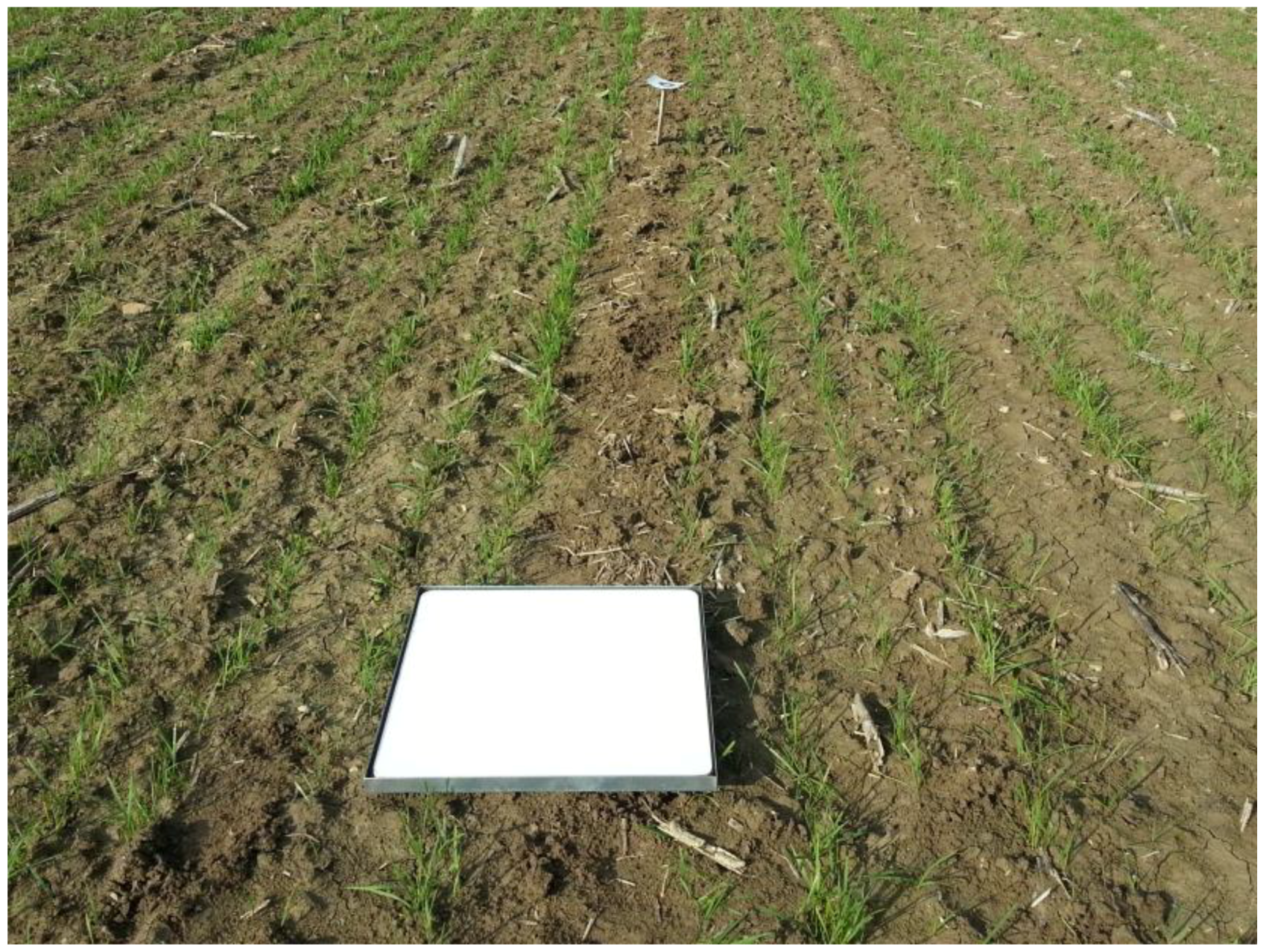
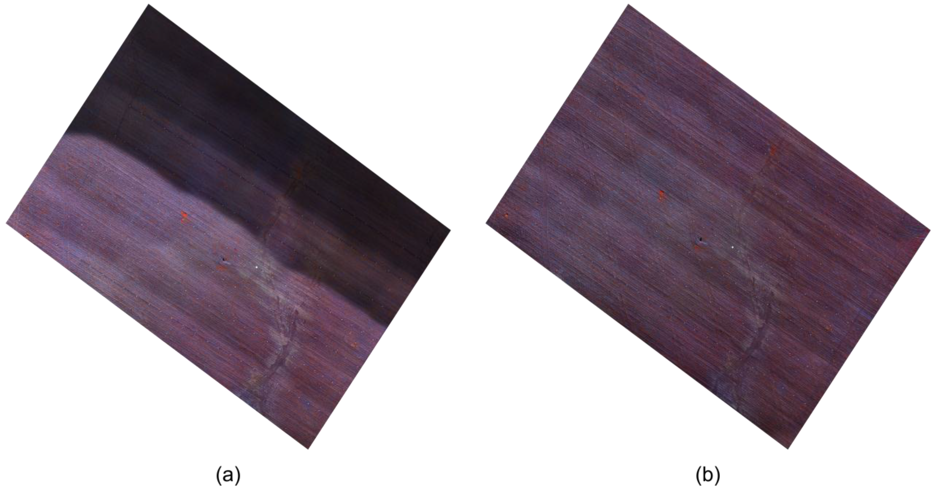
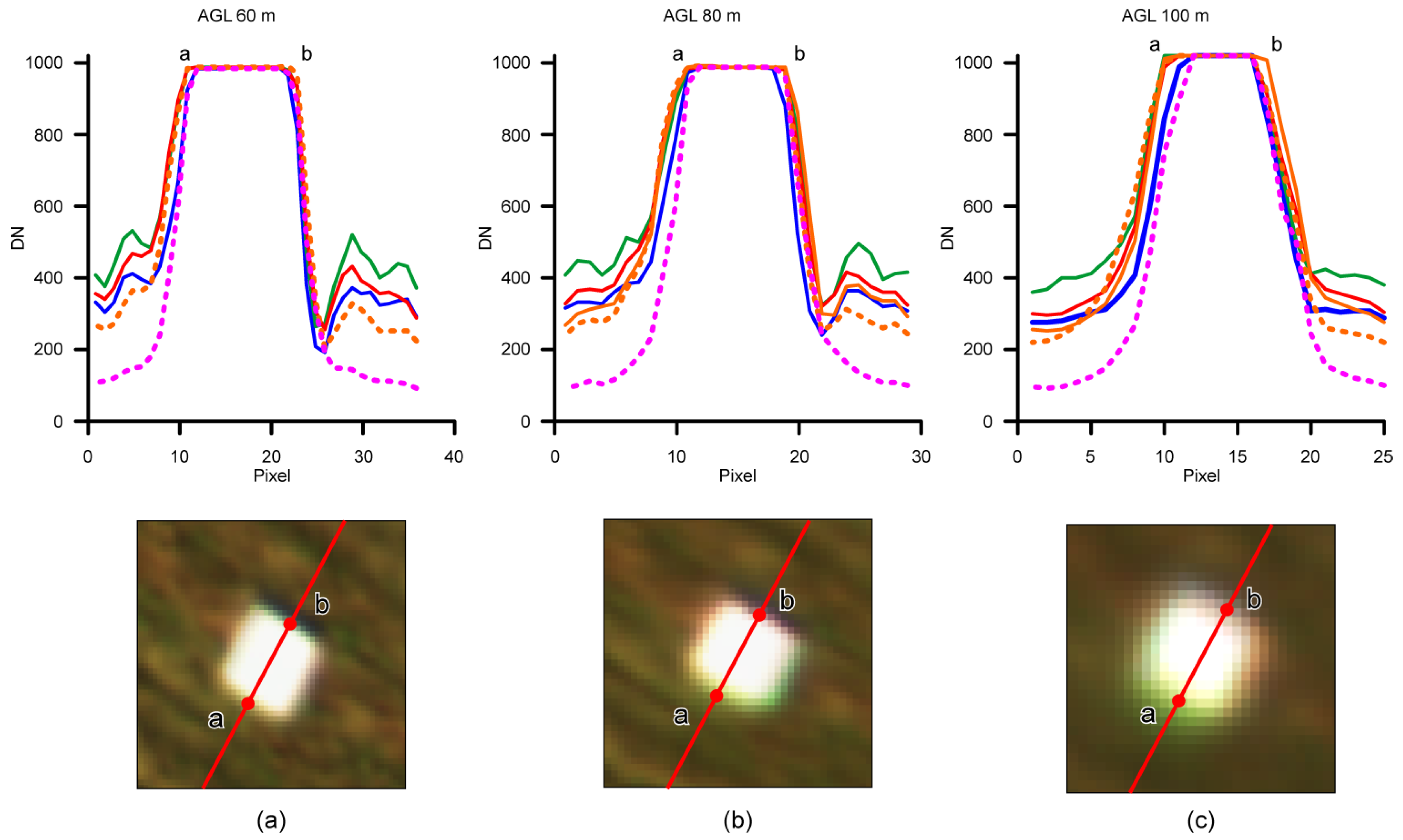
2.4. Assessment of Spatial Resolution

ISO 19157 (2013) [47] defines the spatial accuracy as the accuracy of the position of features in relation to Earth. Spatial accuracy can be described as absolute or relative. Absolute accuracy corresponds to the closeness of reported coordinate values to values accepted as or being true. Relative accuracy is defined as the closeness of the relative spatial positions of features in a dataset to their respective relative spatial positions accepted as or being true. In addition, ISO considers gridded data such as orthomosaicked images. In these cases, gridded data position accuracy is the closeness of the gridded data spatial position values to values accepted as or being true.

Previous to the UAV flights, because user risk is a function of sample size [48], 150 check points were distributed in the area to assess the absolute and relative spatial accuracies. Check points were well-defined points corresponding to targets of 14 × 14 cm (Figure 2b). The check points were placed in a grid distribution of 5 × 11 m (Figure 2a). The coordinates of the check points were obtained using the same methodology described for GCPs (Figure 2c). These coordinates were used as the ground reference values. Check points were digitized, considering each orthomosaicked image produced. These coordinates were obtained using Arcmap 10.1 software (Esri, Redlands, CA, USA). Both sets of coordinates were used to determine the spatial accuracy.

Absolute positional accuracy was assessed considering Root Mean Square Error (RMSE). RMSE is used as an estimator of positional accuracy as developed by the American Society for Photogrammetry and Remote Sensing [49]. RMSEs were calculated considering the total area and a security margin of 10% over the perimeter delimited by the GCP located at the corner. The latter configuration corresponds to flight planning for a manned aerial platform, where limit area is extended over the boundary as a security margin to guarantee spatial accuracy [50]. This extension will reveal whether the number of GCPs also influences the location with respect to the area of interest flown over in the case of UAV.

As a reference to assess the relative positional accuracy, the methodology developed by the Department of Defense of the United States (1990) [51] was followed, and all the possible check point pair combinations were determined. The absolute errors in the X and Y dimensions of each check point and, subsequently, the relative errors in X and Y for all the check point combinations were calculated. These errors were used to calculate both the relative standard deviations on each axis $({\sigma }_{x\_rel}, {\sigma }_{y\_rel})$ and the relative horizontal standard deviation (RHSD).

Figure 2. Details of assessment of spatial resolution: (a) Distribution of ground control check points; (b) sample of distribution over the study site; and (c) measurement by GNSS receiver.

Figure 2. Details of assessment of spatial resolution: (a) Distribution of ground control check points; (b) sample of distribution over the study site; and (c) measurement by GNSS receiver.

2.5. Assessment of Spectral Discrimination

Two types of controls were applied on the orthomosaicked images: (i) multispectral band alignment and (ii) spectral discrimination. Tetracam mini MCA-6 takes the images of each spectral band using an independent sensor. From a photogrammetric point of view, each sensor is independent because each sensor has different internal and external parameters. This approach involves calculating six individual aerial triangulations and, consequently, the band alignment can show some small displacement between bands. The quality of alignment of each orthophoto was evaluated with the help of the spectralon panel placed in the center of the study area (Figure 3). Spatial profiles were taken across the spectralon panel for each orthophoto produced. Each spatial profile represents the spectral values for each band. Data were obtained using the ENVI image processing software (Research System, Inc., Boulder, CO, USA).

The spectral discrimination test was focused on the analysis of the potential effect of UAV flight parameters on the discrimination of different soil covers by incorporating a methodology to produce weed mapping based on UAV images. Two phases are required [8]: (1) bare soil and vegetation discrimination and (2) crop and weed discrimination. The first phase produces an image with two classes: bare soil and vegetation (crop and weeds together). The second phase masks crop and weeds. To determine the influence of UAV flight parameters on weed mapping, spectral values of bare soil, crop and weeds were extracted. These spectral values were collected in 15 random samples for each cover from all the orthomosaicked images produced. Then, the NDVI was derived from these spectral values. The potential of NDVI for spectral discrimination was evaluated by applying the M-Statistic [52] (Equation (1)), where µ and σ are, respectively, the means and standard deviations of class 1 and 2. The M-statistic defines the degree of discrimination between two classes, evaluating the separation between their histograms. A value of M lower than 1 means that histograms overlap significantly, therefore offering poor discrimination. A value of M higher than 1 means histograms are well separated, providing easier discrimination.

$$M=\left({\mu }_{class1}-{\mu }_{class2}\right)/\left({\sigma }_{class1}+{\sigma }_{class2}\right)$$

(1)

Figure 3. Details of experiment setup to assess spectral discrimination: Spectralon panel placed in the middle of the study area.

Figure 3. Details of experiment setup to assess spectral discrimination: Spectralon panel placed in the middle of the study area.

3. Results

Table 1 summarizes the duration, route length and wind speed of each UAV flight considering altitude AGL and mode of flight. Table 1 shows how, as altitude AGL increases, duration of flight is reduced because the increased altitude AGL makes it possible to cover more field crop area. Moreover, if the UAV platform flies in cruising mode, the optimization of the battery is even higher than that in stop mode. The duration of flight ratio considering stop and cruising modes shows a ratio of 4:1, considering the same altitude AGL. The longest duration of UAV flight corresponded to 60 m AGL flying in stop mode, with 38 min 11 sec because it was not possible to perform the whole flight mission with one battery, so we divided the mission into two different flights, motivated by the need to change batteries between flights. Under these circumstances, it is possible to show changes in illumination or in the environmental conditions, which would be reproduced on the registered images. As an example, Figure 4a shows results for 60 m AGL using stop mode flight. The two areas corresponding to both flights are well defined. Figure 4b displays the results considering the same altitude AGL flying in cruising mode. In this case, there were no spectral differences because only one flight was conducted. The shortest flight was obtained for 100 m AGL flying in cruising mode, with 3 min 40 sec. Finally, Table 1 shows all flights were made under same wind speed conditions. The minimum wind speed was 0.8 m/s corresponding to 60 m AGL and stop mode while maximum value was 1.9 for 100 m AGL in cruising mode. Therefore, the results depend only on the technical parameters.

Table 1. Summary of unmanned aerial vehicle (UAV) flights.

		Flight Duration		Wind Speed (m/s)
AGL (m)	Route Length (m)	Stop Mode	Cruising Mode	Stop Mode	Cruising Mode
60	10,740	38 min 11 s	9 min 28 s	0.8	1.3
80	8045	18 min 24 s	4 min 46 s	1.3	1.8
100	9254	11 min 56 s	3 min 40 s	1.8	1.9

Table 1. Summary of unmanned aerial vehicle (UAV) flights.

		Flight Duration		Wind Speed (m/s)
AGL (m)	Route Length (m)	Stop Mode	Cruising Mode	Stop Mode	Cruising Mode
60	10,740	38 min 11 s	9 min 28 s	0.8	1.3
80	8045	18 min 24 s	4 min 46 s	1.3	1.8
100	9254	11 min 56 s	3 min 40 s	1.8	1.9

Figure 4. Effect of UAV flight over an area with (a) different flights or (b) one flight.

Figure 4. Effect of UAV flight over an area with (a) different flights or (b) one flight.

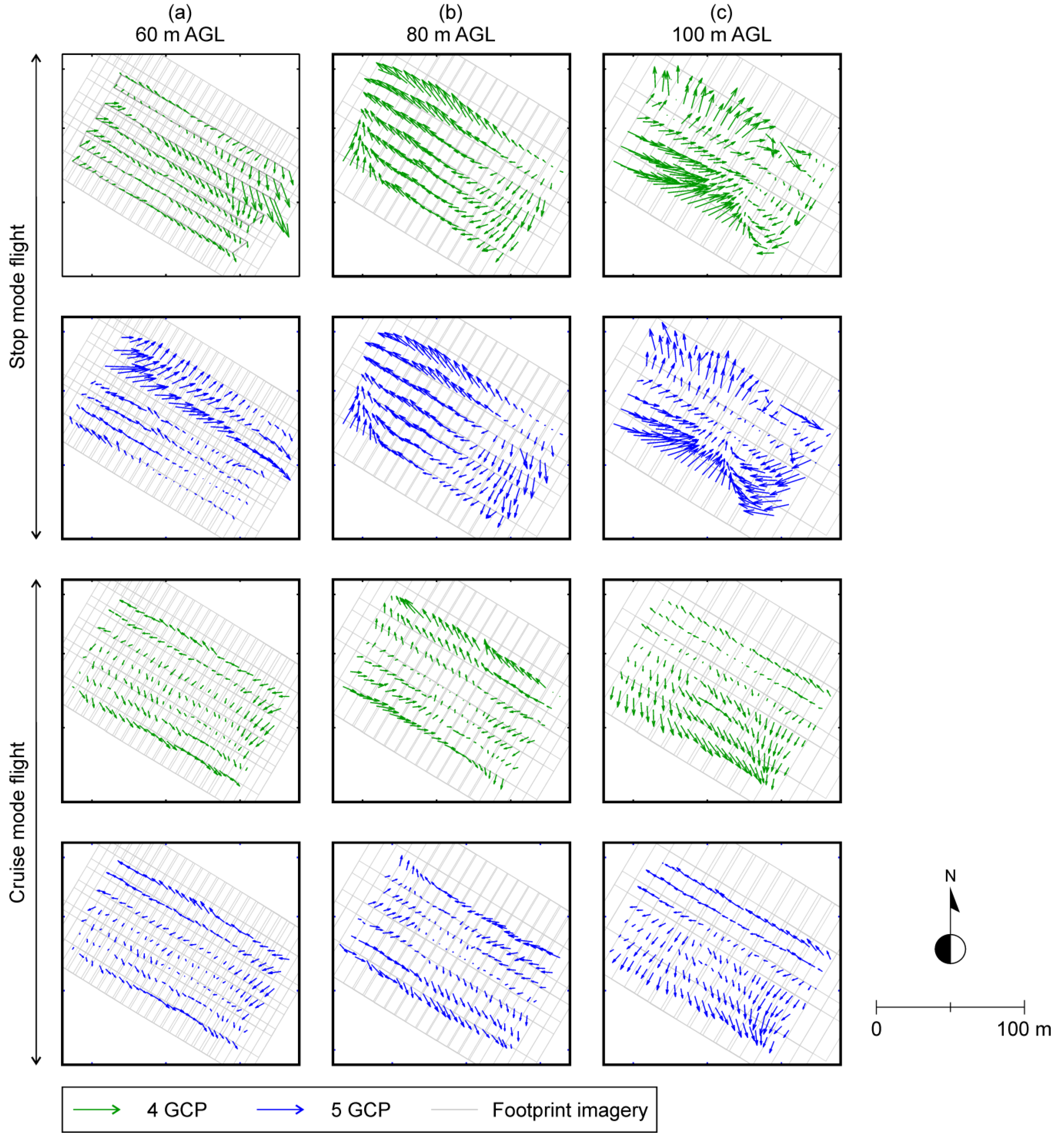
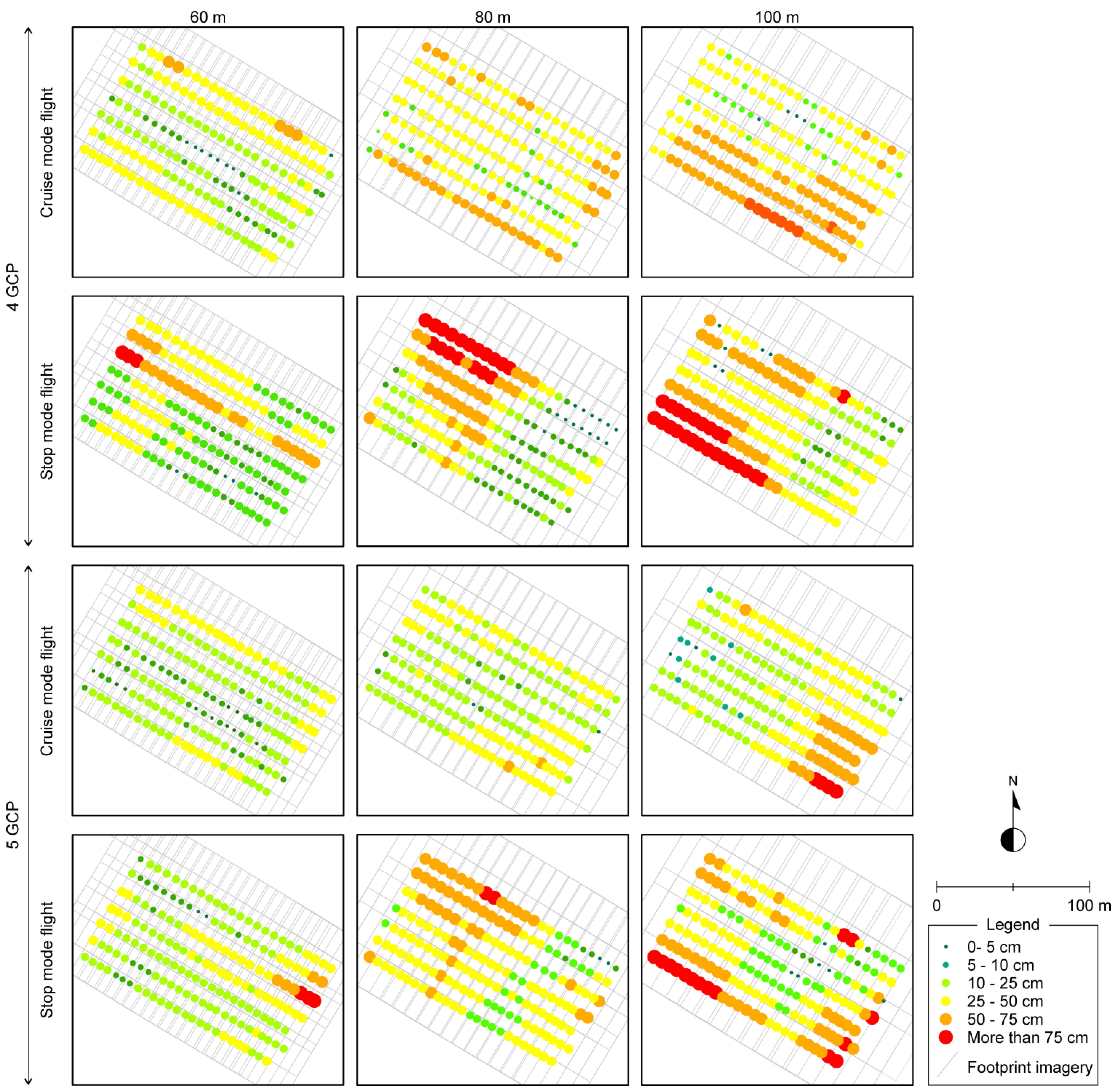
3.1. Effect of UAV Flights Parameters on Orthophoto Spatial Resolution

Table 2 summarizes the results of the absolute spatial resolution assessment considering (1) altitude AGL; (2) flight mode; and (3) number of GCPs. Figure 5 contains a vector error plot graph for each UAV flight to show the spatial distribution and orientation of errors. Errors presented a broad range of values, from 5 cm flying at 60 m AGL in cruising mode to 28.8 cm at 100 m AGL in stop mode. Considering altitude AGL, error increases as altitude AGL increases in all the cases. This behavior is constant in all the flights, independent of other factors. Imagery pixel size is proportional to the flight altitude, and as in manned platforms, errors mainly depend on the flying height [53]. A lower altitude AGL flight allows better geometric accuracy. On Figure 5a, corresponding to 60 m AGL flight, vector errors are smaller than vectors on altitude 80 and 100 m AGL images (Figure 5b,c) independently of flight mode.

Referring to flight mode, vector error graphs for cruising mode flights (Figure 5 “cruise mode flight”) showed smaller vectors than stop mode flights (Figure 5 “stop mode flight”). Considering the full area of study, the error range in cruising mode was from 8.3 to 13.5 cm, whereas for stop mode errors were from 14.5 to 28.8 cm. As in [22], all individual UAV flights in cruising mode have better results than the corresponding version in stop mode. These better results are achieved because, in stop mode, a multi-rotor UAV has more difficulty in maintaining flight direction and the defined forward-lap and side-lap than flights in cruising mode. This circumstance can cause a reduction in the percentage of forward-lap and side-lap, among other factors. The consequence is that the SfM algorithms used to process UAV flights do not work as well as they should [54]. Moreover, the error range considering altitude AGL is lower flying in cruising mode than in stop mode.

Table 2. Results for absolute spatial resolution considering altitude Above Ground Level (AGL), number and distribution of ground control points (GCPs), flight mode and area of interest (FA: Full Area; SM: Security Margin 10%).

AGL (m)	Flight Mode	4 GCPs RMSE (cm)		5 GCPs RMSE (cm)
		FA	SM	FA	SM
60	Stop	14.7	11.6	14.5	11.7
	Cruising	9.8	5.1	8.3	5.3
80	Stop	16.6	14.7	16.4	14. 3
	Cruising	13.1	9.3	8.5	6.3
100	Stop	28.8	18.2	23.2	16.5
	Cruising	13.5	12.1	9.7	9.2

Table 2. Results for absolute spatial resolution considering altitude Above Ground Level (AGL), number and distribution of ground control points (GCPs), flight mode and area of interest (FA: Full Area; SM: Security Margin 10%).

AGL (m)	Flight Mode	4 GCPs RMSE (cm)		5 GCPs RMSE (cm)
		FA	SM	FA	SM
60	Stop	14.7	11.6	14.5	11.7
	Cruising	9.8	5.1	8.3	5.3
80	Stop	16.6	14.7	16.4	14. 3
	Cruising	13.1	9.3	8.5	6.3
100	Stop	28.8	18.2	23.2	16.5
	Cruising	13.5	12.1	9.7	9.2

Regarding the GCPs factor, errors showed a better distribution using 5GCPs instead of 4GCPs, being more evident in cruising mode (Table 2 columns headed “FA”). A traditional distribution of GCPs in Digital Photogrammetry is to set the GCPs at the corner of the block [14]. This GCP distribution in our UAV flights showed satisfactory results, but this distribution did not present clear improvements when adding a new GCP in the middle of the area of study for all the flights. Figure 6 represents the distribution of the spatial error for each check point, showing how the maximum errors are concentrated around the perimeter of the area flown over for all UAV flights independent of flight mode, altitude AGL and number of GCPs. Under these circumstances, a 10% security margin was defined around the perimeter described by the 4GCPs of the corner. A new area of interest was defined, and a new RMSE was calculated for all the flights considering only check points inside this area (Table 2 columns titled “SM”). In this case, the RMSE was lower, especially in those flights where the errors showed high values. Under these conditions, the influence of the number of GCPs was more evident, being motivated by how UAV flights are processed compared with classic Photogrammetry. UAV processing is used at the start of a relative coordinate system, and GCPs are measured at the end of the process to transform from relative to absolute coordinates, similar to, for example, calculating a rigid body transformation [55]. In this transformation, the number and spatial distribution of GCPs affect orthophoto accuracy [56]. This author concluded that the accuracy of the four corners and some areas of the edges in an image depends on the number of GCPs, which matches with our results.

With respect to relative spatial resolution (Table 3), RHSD is stable when the UAV flies in cruising mode, ranging from 9.5 to 14.8 cm (2–3 pixels). In stop mode, RHSD shows values ranging from 10.8 to 22.7 cm (2–5 pixels). RHSD increases as altitude AGL increases in all cases. Referring to GCPs, flying in cruising mode showed no relevant differences compared to stop mode. In this stop mode, considering 5GCPs supposes an improvement of 10 cm (2 pixels) when flying at 80 and 100 m AGL.

Considering these results, there was a relationship between flight parameters and GCP distribution regarding spatial resolution. For flights in cruising mode, the spatial accuracy of orthophotos was better than that in stop mode. In addition, it was possible to cover more field area. Relative to GCPs, setting 4GCPs at the corner and 1GCP in the center of the area stabilizes the RHSD in 8–10 cm. If GCPs are distributed covering a 10% wider area, the error in the area of interest is equal to 5–6 cm for 60 and 80 m altitude AGL, indicating 1 pixel of error. Therefore, if there was not an energy (battery) limitation, we would recommend flying at 60 m AGL to achieve the best spatial resolution. In contrast, flying at 80 m AGL, the RMSE would be slightly poorer, but this would not have a relevant impact on spatial resolution under this setting, in addition to making it possible to cover more area.

With this configuration it is possible to cover 12 ha at 60 m AGL or 16 ha at 80 m AGL. Therefore, it would be necessary to make a number of flights to cover larger fields. Nowadays, one focus of work and research related to the UAV platforms is to increase time flight, improving autonomy. For that reason, it is important to define the best flight conditions.

Figure 5. Vector error distribution of 6-band multispectral orthophoto taking into account flight mode (cruising and stop mode); 60, 80 and 100 meter altitude AGL; and number of ground control points (GCPs).(a) 60 m AGL; (b) 80 m AGL;(c) 100 m AGL.

Figure 5. Vector error distribution of 6-band multispectral orthophoto taking into account flight mode (cruising and stop mode); 60, 80 and 100 meter altitude AGL; and number of ground control points (GCPs).(a) 60 m AGL; (b) 80 m AGL;(c) 100 m AGL.

Figure 6. Distribution of error considering mode of flight (cruising and stop mode); 60, 80 and 100 m altitude AGL; and number of ground control points (GCPs).

Figure 6. Distribution of error considering mode of flight (cruising and stop mode); 60, 80 and 100 m altitude AGL; and number of ground control points (GCPs).

Table 3. Results for absolute spatial resolution considering altitude AGL, number and distribution of GCPs and flight mode.

AGL (m)	Flight Mode	4 GCPs RMSE (cm)	5 GCPs RMSE (cm)
60	Stop	19.5	18.5
	Cruising	14.5	11.3
80	Stop	21.0	10.8
	Cruising	11.0	9.5
100	Stop	22.7	14.9
	Cruising	14.8	13.5

Table 3. Results for absolute spatial resolution considering altitude AGL, number and distribution of GCPs and flight mode.

AGL (m)	Flight Mode	4 GCPs RMSE (cm)	5 GCPs RMSE (cm)
60	Stop	19.5	18.5
	Cruising	14.5	11.3
80	Stop	21.0	10.8
	Cruising	11.0	9.5
100	Stop	22.7	14.9
	Cruising	14.8	13.5

Considering these results, there was a relationship between flight parameters and GCP distribution regarding spatial resolution. For flights in cruising mode, the spatial accuracy of orthophotos was better than that in stop mode. In addition, it was possible to cover more field area. Relative to GCPs, setting 4GCPs at the corner and 1GCP in the center of the area stabilizes the RHSD in 8–10 cm. If GCPs are distributed covering a 10% wider area, the error in the area of interest is equal to 5–6 cm for 60 and 80 m altitude AGL, indicating 1 pixel of error. Therefore, if there was not an energy (battery) limitation, we would recommend flying at 60 m AGL to achieve the best spatial resolution. In contrast, flying at 80 m AGL, the RMSE would be slightly poorer, but this would not have a relevant impact on spatial resolution under this setting, in addition to making it possible to cover more area.

With this configuration it is possible to cover 12 ha at 60 m AGL or 16 ha at 80 m AGL. Therefore, it would be necessary to make a number of flights to cover larger fields. Nowadays, one focus of work and research related to the UAV platforms is to increase time flight, improving autonomy. For that reason, it is important to define the best flight conditions.

UAV and related technologies are developing quickly with more and more efficiency and currently, the main limitation of UAV multirotor is energy (batteries). However, as the following papers show [57,58], these problems are being addressed by several research groups. Our research does not depend on the crop field size. Therefore it can be applied in the future to UAV equipped with a better energy supplied to fly longer durations.

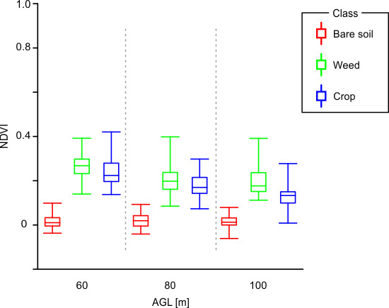
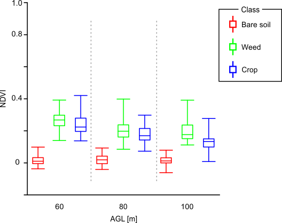
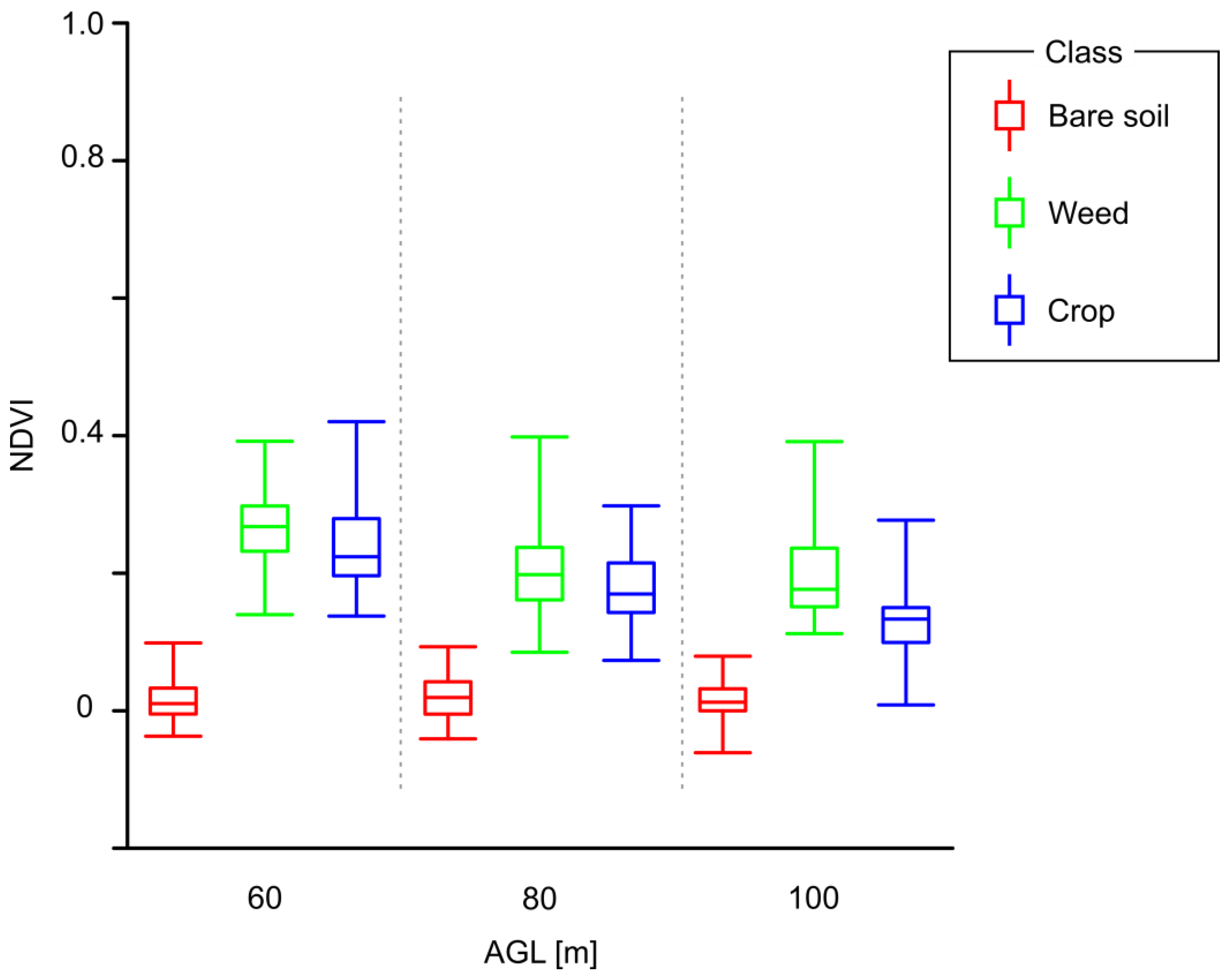
3.2. Effect of UAV Flights Parameters on Orthophoto Spectral Discrimination

The influence of altitude AGL on spectral discrimination was studied by considering UAV flights in cruising mode and 5GCPs as the optimum setting to obtain the best spatial resolution. A new orthomosaicked image for each altitude AGL was produced in which the GSD was related to altitude AGL. As a result, the new GSD orthomosaicked image values were 3, 4 and 5 cm×pixel⁻¹ for 60, 80 and 100 m altitude AGL, respectively. Figure 7 shows a subset, including the spectralon panel, of each orthomosaicked image accompanied by an axis (red line) used to extract a spectral profile of each spectral band at 10-bit radiometric resolution. Although the multispectral camera registers each image using six individual sensors, there was no evidence of misalignment between bands in any flight. At 60 m AGL (Figure 7a), the orthomosaicked image showed well defined objects with clear borders. In this case, the transition from shadows to the spectralon panel (point b in the profile) was almost a vertical line. The transition from the spectralon panel to bare soil (point a in the profile) was not a vertical line, as was recorded in the previous point, possibly because the spectral response of each band is different while the above shadow has a constant response. Moreover, considering a visual analysis, crop lines were well defined. At 80 m AGL (Figure 7b), the spectralon panel showed more diffuse borders, and furthermore, the crop rows were more poorly defined, showing a blurred aspect because the response of an individual pixel is a radiometric measurement arising from a two dimensional spatially extended region of the field of view [59]. Therefore, as altitude AGL increases, GSD also increases. The increase involves increasing the field of view and, hence, a worse definition of the spectral curves. Altitude AGL equal to 100 m (Figure 7c) showed the worst transition between objects. The spectralon panel exhibited a scattered definition, and crop rows practically disappeared.

Figure 7. Spatial (upper figures) and spectral (lower figures) profiles over orthomosaicked images at (a) 60, (b) 80 and (c) 100 m altitude AGL.

Figure 7. Spatial (upper figures) and spectral (lower figures) profiles over orthomosaicked images at (a) 60, (b) 80 and (c) 100 m altitude AGL.

On a second stage, spectral discrimination between bare soil, crop and weeds was studied. Table 4 shows the range and average spectral pixel values of the NDVI of each class considering 60, 80 and 100 m AGL. In ESSWM, a first stage is focused on distinguishing between bare soil and vegetation. Figure 8 represents M-statistics values for each class and altitude AGL. At 60 m AGL, the M-statistic showed the best separation between vegetation (crop and weeds) and bare soil (M = 2.74, Table 5). This result offers a robust separability among classes. At 80 and 100 m AGL, the results (M = 1.86 and 1.55, respectively) were not as satisfactory as at 60 m AGL. The results were higher than 1, so separability of classes is a priori adequate, although a higher GSD decreases the M-statistic. Therefore, increasing the altitude AGL affects the separability negatively. Figure 8 displays how boxes representing weeds and crops are closer to bare soil boxes at 80 and 100 m AGL than at 60 m AGL. Referring to the separation between crop and weeds, M-values were lower than 1, considering all the altitude AGLs (Table 5). Figure 8 shows how both boxes were quite similar, and these classes were therefore not well distinguished. The best M-value was obtained at 100 m AGL, one reason being that GSD is higher and pixels of bare soil are mixed, particularly in the case of weeds.

Table 4. NDVI statistics for the classes: vegetation (V, including weed and crop), weed (W), crop (C) and bare soil (B).

NDVI	60 m AGL				80 m AGL				100 m AGL
Statistics	V	W	C	B	V	W	C	B	V	W	C	B
Minimum	0.14	0.14	0.13	−0.03	0.07	0.08	0.07	−0.04	0.01	0.11	0.01	−0.03
Maximum	0.42	0.39	0.42	0.09	0.40	0.39	0.29	0.09	0.39	0.39	0.27	0.07
Deviation	0.06	0.05	0.06	0.02	0.06	0.07	0.05	0.02	0.07	0.06	0.05	0.02
Mean	0.25	0.26	0.24	0.01	0.20	0.21	0.18	0.02	0.17	0.19	0.13	0.01
Median	0.25	0.26	0.22	0.01	0.19	0.19	0.17	0.01	0.02	0.17	0.13	0.01

Table 4. NDVI statistics for the classes: vegetation (V, including weed and crop), weed (W), crop (C) and bare soil (B).

NDVI	60 m AGL				80 m AGL				100 m AGL
Statistics	V	W	C	B	V	W	C	B	V	W	C	B
Minimum	0.14	0.14	0.13	−0.03	0.07	0.08	0.07	−0.04	0.01	0.11	0.01	−0.03
Maximum	0.42	0.39	0.42	0.09	0.40	0.39	0.29	0.09	0.39	0.39	0.27	0.07
Deviation	0.06	0.05	0.06	0.02	0.06	0.07	0.05	0.02	0.07	0.06	0.05	0.02
Mean	0.25	0.26	0.24	0.01	0.20	0.21	0.18	0.02	0.17	0.19	0.13	0.01
Median	0.25	0.26	0.22	0.01	0.19	0.19	0.17	0.01	0.02	0.17	0.13	0.01

Table 5. M-Statistics between crop and weed, bare soil and weed, bare soil and crop and bare soil and vegetation (including crop and weed).

Classes	60 m		80 m		100 m
	Crop	Bare Soil	Crop	Bare Soil	Crop	Bare Soil
Weed	0.23	3.06	0.24	1.88	0.52	1.92
Crop	-	2.51	-	1.94	-	1.38
Vegetation	-	2.74	-	1.86	-	1.55

Table 5. M-Statistics between crop and weed, bare soil and weed, bare soil and crop and bare soil and vegetation (including crop and weed).

Classes	60 m		80 m		100 m
	Crop	Bare Soil	Crop	Bare Soil	Crop	Bare Soil
Weed	0.23	3.06	0.24	1.88	0.52	1.92
Crop	-	2.51	-	1.94	-	1.38
Vegetation	-	2.74	-	1.86	-	1.55

Figure 8. NDVI values for the classes of bare soil, weed and crop, considering flights at 60, 80 and 100 m altitude AGL.

Figure 8. NDVI values for the classes of bare soil, weed and crop, considering flights at 60, 80 and 100 m altitude AGL.

Using this spectral information, it is, therefore, possible to distinguish between bare soil and vegetation considering all the altitude AGLs, but it was not possible to discriminate between weeds and crop. Once our results demonstrated the generation of high quality orthomosaicks, this spectral similarity could be resolved using the object-based image analysis (OBIA) methodology [56]. The OBIA methodology uses spectral, textural and hierarchical features after segmentation of imagery acquired for other herbaceous crops such as maize and sunflowers [60]. In this context, weed patches can be distinguished from crop plants using the relative position instead of only spectral information. For that distinction, it is necessary to first determine the crop rows, and then, every plant that is not located in these crop lines can be considered a weed. Altitude AGL can also be a parameter to consider for the results on crop line detection. As part of an overall research programme, which investigates the possibilities and limitations of UAV imagery to support site-specific crop management, it is crucial to explore the potential of generating accurate orthomosaicks from UAV flights for proper discrimination of weeds using a multispectral sensor. Such an approach should demonstrate the potential of the orthomosaicks generated and their accuracy for further weed discrimination. The ultimate objective of our work is to generate weed maps using these multispectral orthomosaicks. These maps, which provide the required georreferenced information, will then be used in the decision-making process to design the site specific herbicide treatment maps which will direct treatment to the weed infested areas only. Therefore it is necessary to produce the best orthomosaicks (mainly in higher spatial resolution) to generate accurate weed maps at early stage for a timely and efficient early post-emergence treatment. For this reason, our research assessed the best setting of UAV flight parameters, i.e., the number and location of GCPs, cruising flight mode and altitude AGL. Following these settings, altitude AGL influences spatial resolution and spectral discrimination of the orthomosaicks. Both are key factors in achieving an adequate segmentation of the image. After the segmentation of the orthomosaicks, the spatially accurate created object would represent only one class and not a mixture of vegetation (crop or weed) and bare soil. Torres-Sánchez et al. (2015) [61] assessed the accuracy of image classification using OBIA algorithms on single UAV images registered on wheat at 30 m AGL using an RGB camera.Future investigation will be focused on determining how the parameter of altitude AGL affects the OBIA methodology results considering orthomosaicked images and a multispectral sensor on a wheat field.

4. Conclusions

The main objectives of this research were to analyze the technical specifications and configuration of a multi-rotor UAV equipped with a multispectral sensor to produce the most accurate ortho-photography considering spatial resolution and spectral discrimination and how these specifications and configuration influence the detection of weeds in a crop. Moreover, to determine the best spatial resolution and spectral discrimination, it was necessary to consider whether UAV platforms were able to cover the whole area of interest. These three conditions were related to UAV flight mission planning, so those parameters must be defined jointly and not isolated.

Considering spatial resolution, flight altitude is an important parameter, not so much for the RMSE obtained as spatial resolution considering other parameters but for the degree of detail achieved in the orthomosaicked image to be processed by further image analysis such as the OBIA methodology. Altitude AGL has a negative impact on the duration of the flight that can be minimized by flying in cruise mode. Therefore, it is possible to fly for less time and cover the full area of interest using only one battery, thus avoiding potential problems related to changing light or weather conditions. Regarding the number and distribution of GCPs, the RMSE is closer to the GSD if a security margin can be considered, so we would recommend covering more than the area of interest and placing the GCPs in that margin. Thus, the study area has an error range lower than the adjacent areas close to the field perimeter. Considering spectral discrimination, flight altitude is an important parameter depending on the type of processing developed for the orthomosaicked image. Considering spectral differences between vegetation (including crop and weeds), all the altitudes AGL showed satisfactory results. At the same time, none altitude AGL let to difference between crop and weeds from a spectral point of view. One solution to improve this classification would be to use OBIA methodology.

Therefore, the best setting to maximize spatial resolution and spectral discrimination is to define a flight planning with 10% of security margin, to fly in cruising mode at 60 m altitude AGL and to use 5GCPs.

The results and methodology herein presented can be used to configure flight mission using a multiple-array or a single sensor on-board a multi-rotor UAV to maximize the spatial resolution and spectral discrimination of orthomosaicked image to use in precision agriculture.

References

1. Srbinovska, M.; Gavrovski, C.; Dimcev, V.; Krkoleva, A.; Borozan, V. Environmental parameters monitoring in precision agriculture using wireless sensor networks. J. Clean. Prod. 2015, 88, 297–307. [Google Scholar] [CrossRef]
2. Mulla, D.J. Twenty five years of remote sensing in precision agriculture: Key advances and remaining knowledge gaps. Biosyst. Eng. 2013, 114, 358–371. [Google Scholar] [CrossRef]
3. Ge, Y.; Thomasson, J.A.; Sui, R. Remote sensing of soil properties in precision agriculture: A review. Front. Earth Sci. 2011, 5, 229–238. [Google Scholar] [CrossRef]
4. De Castro, A.; López-Granados, F.; Jurado-Expósito, M. Broad-scale cruciferous weed patch classification in winter wheat using QuickBird imagery for in-season site-specific control. Precis. Agric. 2013, 14, 392–413. [Google Scholar] [CrossRef]
5. López-Granados, F.; Jurado-Expósito, M.; Peña-Barragán, J.M.; García-Torres, L. Using geostatistical and remote sensing approaches for mapping soil properties. Eur. J. Agron. 2005, 23, 279–289. [Google Scholar] [CrossRef]
6. Abbas, A.; Khan, S.; Hussain, N.; Hanjra, M.A.; Akbar, S. Characterizing soil salinity in irrigated agriculture using a remote sensing approach. Phys. Chem. Earth 2013, 55–57, 43–52. [Google Scholar] [CrossRef]
7. Laliberte, A.S.; Goforth, M.A.; Steele, C.M.; Rango, A. Multispectral remote sensing from unmanned aircraft: Image processing workflows and applications for rangeland environments. Remote Sens. 2011, 3, 2529–2551. [Google Scholar] [CrossRef]
8. López-Granados, F. Weed detection for site-specific weed management: Mapping and real-time approaches. Weed Res. 2011, 51, 1–11. [Google Scholar] [CrossRef]
9. Zhang, C.; Kovacs, J. The application of small unmanned aerial systems for precision agriculture: A review. Precis. Agric. 2012, 13, 693–712. [Google Scholar] [CrossRef]
10. Rango, A.; Laliberte, A.; Steele, C.; Herrick, J.E.; Bestelmeyer, B.; Schmugge, T.; Roanhorse, A.; Jenkins, V. Using unmanned aerial vehicles for rangelands: Current applications and future potentials. Environ. Pract. 2006, 8, 159–168. [Google Scholar] [CrossRef]
11. Peña, J.M.; Torres-Sánchez, J.; de Castro, A.I.; Kelly, M.; López-Granados, F. Weed mapping in early-season maize fields using object-based analysis of unmanned aerial vehicle (UAV) images. PLoS ONE 2013, 8, e77151. [Google Scholar]
12. Paparoditis, N.; Souchon, J.-P.; Martinoty, G.; Pierrot-Deseilligny, M. High-end aerial digital cameras and their impact on the automation and quality of the production workflow. ISPRS J. Photogramm. Remote Sens. 2006, 60, 400–412. [Google Scholar] [CrossRef]
13. Markelin, L.; Honkavaara, E.; Hakala, T.; Suomalainen, J.; Peltoniemi, J. Radiometric stability assessment of an airborne photogrammetric sensor in a test field. ISPRS J. Photogramm. Remote Sens. 2010, 65, 409–421. [Google Scholar] [CrossRef]
14. Ackermann, F. Operational Rules and Accuracy Models for GPS-Aerotriangulation. Available online: http://www.isprs.org/proceedings/xxix/congress/part3/691_XXIX-part3.pdf (accessed on 17 June 2015).
15. Müller, J.; Gärtner-Roer, I.; Thee, P.; Ginzler, C. Accuracy assessment of airborne photogrammetrically derived high-resolution digital elevation models in a high mountain environment. ISPRS J. Photogramm. Remote Sens. 2014, 98, 58–69. [Google Scholar] [CrossRef]
16. European Commission Joint Research Centre. Inspire Data Specification for the Spatial Data Theme Orthoimagery. Available online: http://inspire.ec.europa.eu/index.cfm/pageid/2 (accessed on 17 June 2015).
17. Zhang, Y.; Xiong, J.; Hao, L. Photogrammetric processing of low-altitude images acquired by unpiloted aerial vehicles. Photogramm. Rec. 2011, 26, 190–211. [Google Scholar] [CrossRef]
18. Pajares, G. Overview and current status of remote sensing applications based on unmanned aerial vehicles (UAVs). Photogramm. Eng. Remote Sens. 2015, 81, 281–330. [Google Scholar] [CrossRef]
19. Torres-Sánchez, J.; López-Granados, F.; de Castro, A.I.; Peña-Barragán, J.M. Configuration and specifications of an unmanned aerial vehicle (UAV) for early site specific weed management. PLoS ONE 2013, 8, e58210. [Google Scholar] [PubMed]
20. Hengl, T. Finding the right pixel size. Comput. Geosci. 2006, 32, 1283–1298. [Google Scholar] [CrossRef]
21. Peña, J.M.; Torres-Sánchez, J.; Serrano-Pérez, A.; de Castro, A.I.; López-Granados, F. Quantifying efficacy and limits of unmanned aerial vehicle (UAV) technology for weed seedling detection as affected by sensor resolution. Sensors 2015, 15, 5609–5626. [Google Scholar] [CrossRef] [PubMed]
22. Eisenbeiss, H.; Sauerbier, M. Investigation of uav systems and flight modes for photogrammetric applications. Photogramm. Rec. 2011, 26, 400–421. [Google Scholar] [CrossRef]
23. Rodriguez-Gonzalvez, P.; Gonzalez-Aguilera, D.; Lopez-Jimenez, G.; Picon-Cabrera, I. Image-based modeling of built environment from an unmanned aerial system. Automation Constr. 2014, 48, 44–52. [Google Scholar] [CrossRef]
24. Eisenbeiss, H. The autonomous mini helicopter: A powerful platform for mobile mapping. Int. Arch. Photogramm. Remote Sens. Spat. Inf. Sci. 2008, 37, 977–983. [Google Scholar]
25. Wang, J.; Ge, Y.; Heuvelink, G.B.M.; Zhou, C.; Brus, D. Effect of the sampling design of ground control points on the geometric correction of remotely sensed imagery. Int. J. Appl. Earth Obs. Geoinf. 2012, 18, 91–100. [Google Scholar] [CrossRef]
26. Vega, F.A.; Ramírez, F.C.; Saiz, M.P.; Rosúa, F.O. Multi-temporal imaging using an unmanned aerial vehicle for monitoring a sunflower crop. Biosyst. Eng. 2015, 132, 19–27. [Google Scholar] [CrossRef]
27. Turner, D.; Lucieer, A.; Watson, C. An automated technique for generating georectified mosaics from ultra-high resolution unmanned aerial vehicle (UAV) imagery, based on structure from motion (SFM) point clouds. Remote Sens. 2012, 4, 1392–1410. [Google Scholar] [CrossRef]
28. Mesas-Carrascosa, F.J.; Clavero Rumbao, I.; Barrera Berrocal, J.A.; García-Ferrer Porras, A. Positional quality assessment of orthophotos obtained from sensors onboard multi-rotor UAV platforms. Sensors 2014, 14, 22394–22407. [Google Scholar] [CrossRef]
29. Primicerio, J.; di Gennaro, S.; Fiorillo, E.; Genesio, L.; Lugato, E.; Matese, A.; Vaccari, F. A flexible unmanned aerial vehicle for precision agriculture. Precis. Agric. 2012, 13, 517–523. [Google Scholar] [CrossRef]
30. Hruska, R.; Mitchell, J.; Anderson, M.; Glenn, N.F. Radiometric and geometric analysis of hyperspectral imagery acquired from an unmanned aerial vehicle. Remote Sens. 2012, 4, 2736–2752. [Google Scholar] [CrossRef]
31. Möller, M.; Alchanatis, V.; Cohen, Y.; Meron, M.; Tsipris, J.; Naor, A.; Ostrovsky, V.; Sprintsin, M.; Cohen, S. Use of thermal and visible imagery for estimating crop water status of irrigated grapevine. J. Exp. Bot. 2007, 58, 827–838. [Google Scholar] [CrossRef] [PubMed]
32. Gómez-Candón, D.; de Castro, A.I.; López-Granados, F. Assessing the accuracy of mosaics from unmanned aerial vehicle (UAV) imagery for precision agriculture purposes in wheat. Precis. Agric. 2014, 15, 44–56. [Google Scholar] [CrossRef]
33. Torres-Sánchez, J.; Peña, J.M.; de Castro, A.I.; López-Granados, F. Multi-temporal mapping of the vegetation fraction in early-season wheat fields using images from UAV. Comput. Electron. Agric. 2014, 103, 104–113. [Google Scholar] [CrossRef]
34. Hunt, E.R.; Hively, W.D.; Fujikawa, S.; Linden, D.; Daughtry, C.S.; McCarty, G. Acquisition of nir-green-blue digital photographs from unmanned aircraft for crop monitoring. Remote Sens. 2010, 2, 290–305. [Google Scholar] [CrossRef]
35. Huang, Y.; Thomson, S.J.; Lan, Y.; Maas, S.J. Multispectral imaging systems for airborne remote sensing to support agricultural production management. Int. J. Agric. Biol. Eng. 2010, 3, 50–62. [Google Scholar]
36. Kelcey, J.; Lucieer, A. Sensor correction of a 6-band multispectral imaging sensor for UAV remote sensing. Remote Sens. 2012, 4, 1462–1493. [Google Scholar] [CrossRef]
37. Tetracam. Pixelwrench 2. Available online: http://www.Tetracam.Com/pdfs/pw2%20faq.Pdf (accessed on 17 June 2015).
38. Meier, U. Growth Stages of Mono- and Dicotyledonous Plants. Bb Monograph. Available online: http://www.bba.de/veroeff/bbch/bbcheng.pdf (accessed on 17 June 2015).
39. Kraus, K. Photogrammetry—Geometry from Images and Laser Scans; Walter de Gruyter: Goettingen, Germany, 2007. [Google Scholar]
40. Lowe, D.G. Distinctive image features from scale-invariant keypoints. Int. J. Comput. Vis. 2004, 60, 91–110. [Google Scholar] [CrossRef]
41. Snavely, N.; Garg, R.; Seitz, S.M.; Szeliski, R. Finding paths through the world’s photos. ACM Trans. Graph. 2008, 27, 1–11. [Google Scholar] [CrossRef]
42. Aber, J.S.; Marzolff, I.; Ries, J.B. Chapter 3—Photogrammetry. In Small-Format Aerial Photography; Ries, J.S.A.M.B., Ed.; Elsevier: Amsterdam, The Netherlands, 2010; pp. 23–39. [Google Scholar]
43. Fischler, M.A.; Bolles, R.C. Random sample consensus: A paradigm for model fitting with applications to image analysis and automated cartography. Commun. ACM 1981, 24, 381–395. [Google Scholar] [CrossRef]
44. Bemis, S.P.; Micklethwaite, S.; Turner, D.; James, M.R.; Akciz, S.; Thiele, S.T.; Bangash, H.A. Ground-based and UAV-based photogrammetry: A multi-scale, high-resolution mapping tool for structural geology and paleoseismology. J. Struct. Geol. 2014, 69, 163–178. [Google Scholar] [CrossRef]
45. Seitz, S.M.; Curless, B.; Diebel, J.; Scharstein, D.; Szeliski, R. A Comparison and Evaluation of Multi-View Stereo Reconstruction Algorithms. In Proceedings of the 2006 IEEE Computer Society Conference on Computer Vision and Pattern Recognition, 17–22 June 2006; pp. 519–528.
46. Furukawa, Y.; Ponce, J. Accurate, dense, and robust multiview stereopsis. IEEE Trans. Pattern Anal. Mach. Intell. 2010, 32, 1362–1376. [Google Scholar] [CrossRef] [PubMed]
47. International Organization for Standardization (ISO). Geographic Information—Data Quality; ISO: London, UK, 2013. [Google Scholar]
48. Ariza Lopez, F.J.; Atkinson Gordo, A.D.; Rodriguez Avi, J. Acceptance curves for the positional control of geographic databases. J. Surv. Eng. 2008, 134, 26–32. [Google Scholar] [CrossRef]
49. American Society of Photogrammetry and Remote Sensing (ASPRS). ASPRS Positional Accuracy Standards for Digital Geospatial Data; ASPRS: Bethesda, MA, USA, 2014. [Google Scholar]
50. US Army Corps of Engineers (USACE). Engineering and Design. Photogrammetric Mapping; USACE: Washington, DC, USA, 2002. [Google Scholar]
51. Practice, D.O.D.S. Mapping, Charting and Geodesy Accuracy. Available online: http://earth-info.nga.mil/publications/specs/printed/600001/600001_Accuracy.pdf (accessed on 25 September 2015).
52. Kaufman, Y.J.; Remer, L.A. Detection of forests using mid-IR reflectance: An application for aerosol studies. IEEE Trans. Geosci. Remote Sens. 1994, 32, 672–683. [Google Scholar] [CrossRef]
53. Baltsavias, E.P. A comparison between photogrammetry and laser scanning. ISPRS J. Photogramm. Remote Sens. 1999, 54, 83–94. [Google Scholar] [CrossRef]
54. Ruzgienė, B.; Berteška, T.; Gečyte, S.; Jakubauskienė, E.; Aksamitauskas, V.Č. The surface modelling based on uav photogrammetry and qualitative estimation. Measurement 2015, 73, 619–627. [Google Scholar]
55. Westoby, M.J.; Brasington, J.; Glasser, N.F.; Hambrey, M.J.; Reynolds, J.M. “Structure-from-motion” photogrammetry: A low-cost, effective tool for geoscience applications. Geomorphology 2012, 179, 300–314. [Google Scholar] [CrossRef] [Green Version]
56. Orti, F. Optimal distribution of control points to minimize Landsat image registration errors. Photogramm. Eng. Remote Sens. 1981, 47, 101–110. [Google Scholar]
57. Verbeke, J.; Hulens, D.; Ramon, H.; Goedeme, T.; de Schutter, J. The design and construction of a high endurance hexacopter suited for narrow corridors. In Proceedings of the 2014 International Conference on Unmanned Aircraft Systems (ICUAS), Orlando, FL, USA, 27–30 May 2014; pp. 543–551.
58. Gatti, M.; Giulietti, F. Preliminary design analysis methodology for electric multirotor. In Proceedings of the RED-UAS 2013, 2nd IFAC Workshop Research, Education and Development of Unmanned Aerial Systems, Compiegne, France, 20–22 November 2013; pp. 58–63.
59. Forster, B.C.; Best, P. Estimation of spot p-mode point spread function and derivation of a deconvolution filter. ISPRS J. Photogramm. Remote Sens. 1994, 49, 32–42. [Google Scholar] [CrossRef]
60. Peña-Barragán, J.M.; Ngugi, M.K.; Plant, R.E.; Six, J. Object-based crop identification using multiple vegetation indices, textural features and crop phenology. Remote Sens. Environ. 2011, 115, 1301–1316. [Google Scholar] [CrossRef]
61. Torres-Sánchez, J.; López-Granados, F.; Peña, J.M. An automatic object-based method for optimal thresholding in UAV images: Application for vegetation detection in herbaceous crops. Comput. Electron. Agric. 2015, 114, 43–52. [Google Scholar] [CrossRef]