
Accuracy Optimization for High Resolution Object-Based Change Detection: An Example Mapping Regional Urbanization with 1-m Aerial Imagery

Abstract
:
1. Introduction
1.1. Objectives
1.1.1. Object-Based Image Analysis and Change Detection
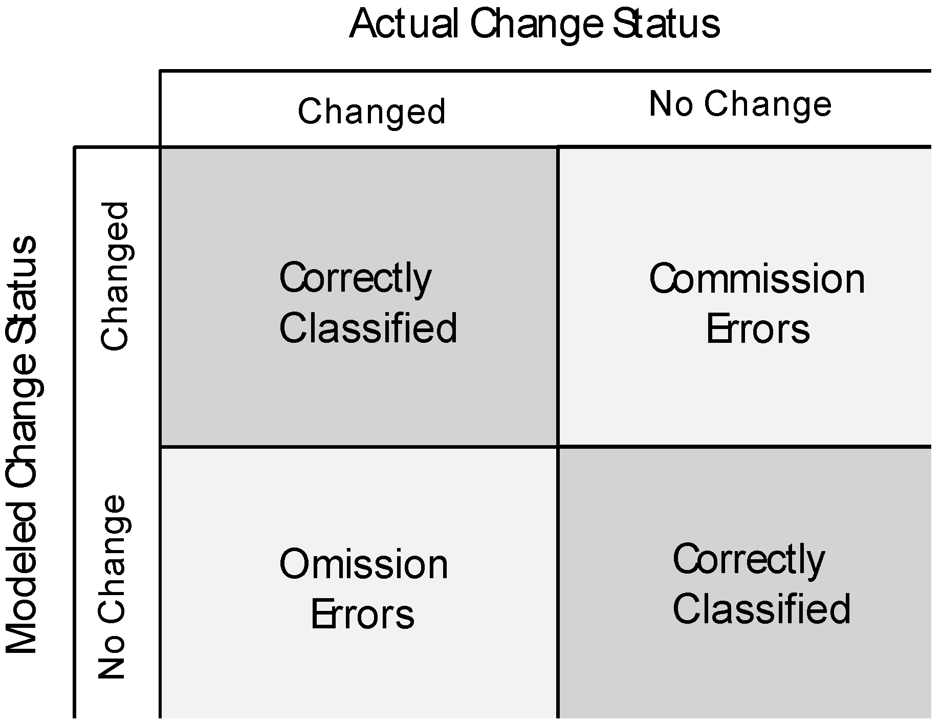
1.1.2. Accuracy Assessment
1.1.3. Accuracy Optimization
2. Methods
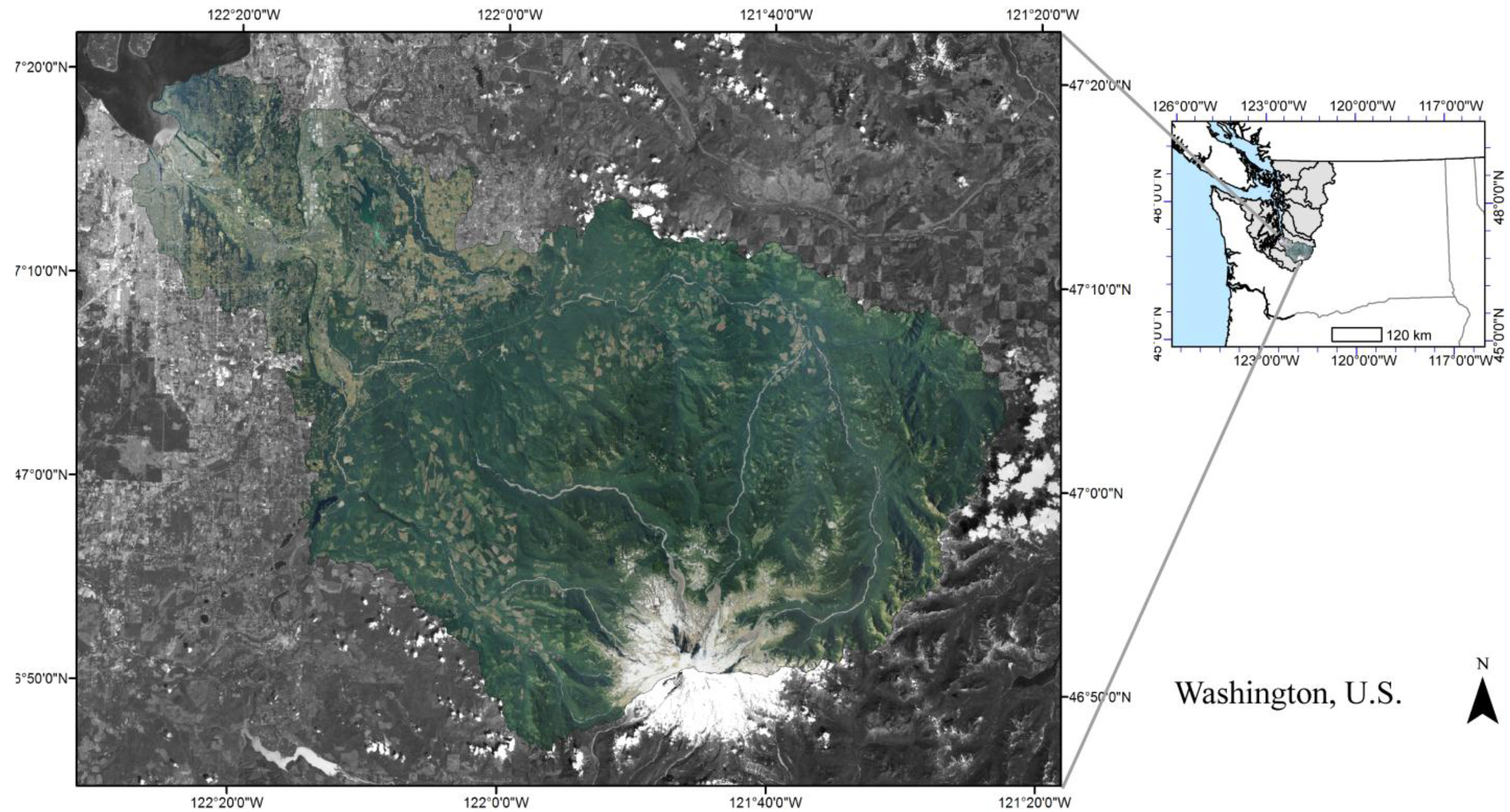
2.1. Study Area

2.2. Image Data Processing
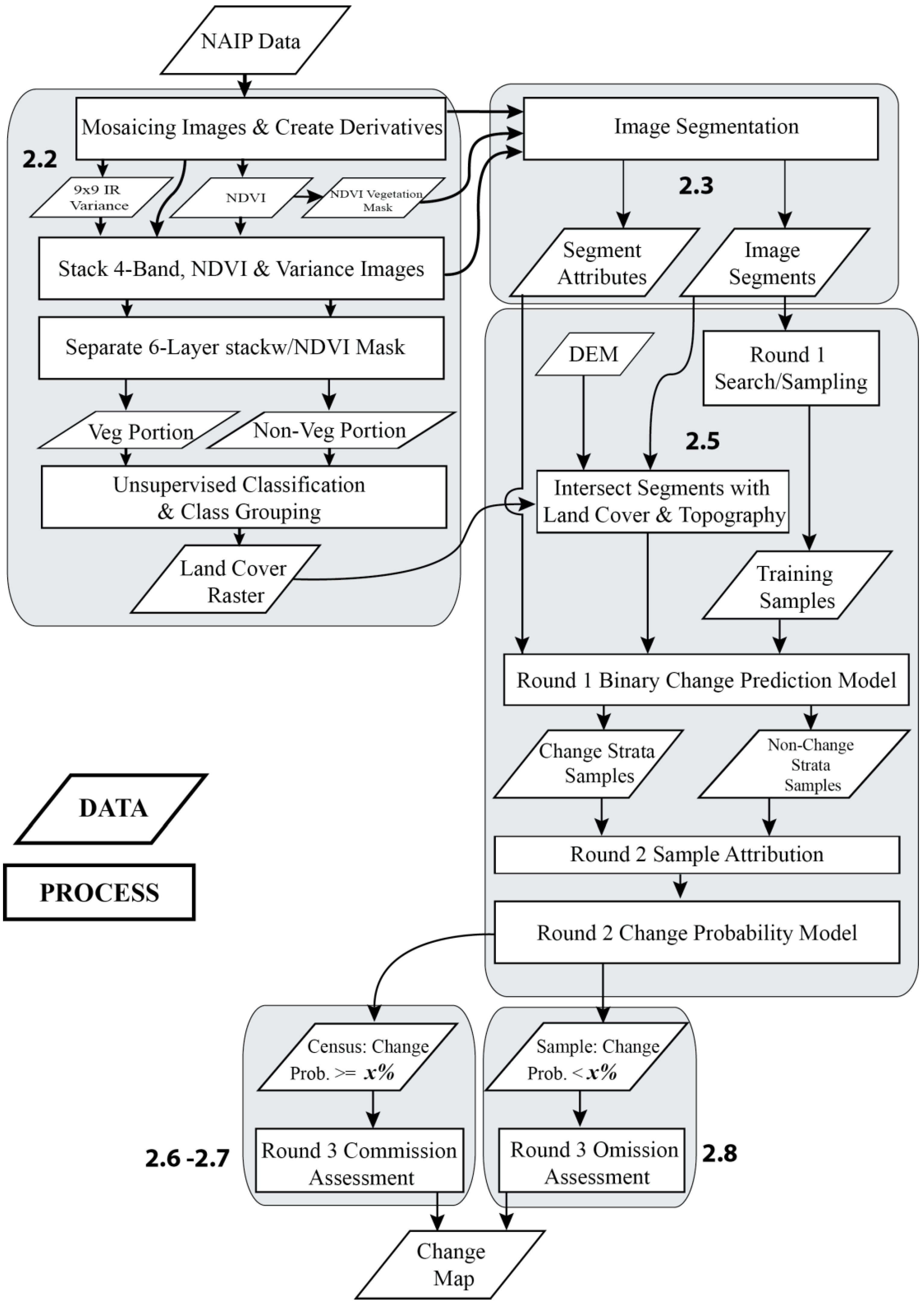
2.3. Segment Generation

| # | Polygon Attributes | Type/Units |
|---|---|---|
| 1–3 | 2006 Bands: Red, Green, Blue | Polygon Mean |
| 4–6 | 2009 Bands: Red, Green, Blue | Polygon Mean |
| 7 | 2009 Band 4: Infrared | Polygon Mean |
| 8 | 2009 Derived: NDVI | Polygon Mean |
| 9–11 | 2009–2006 Difference: Red, Green, Blue | Polygon Mean |
| 12–22 | Same as 1–11 | Polygon St. Deviation |
| 23 | Contrast neighbor 2006 Red | Contrast across polygon border |
| 24 | Contrast neighbor 2009 Red | Contrast across polygon border |
| 25–26 | 2006, 2009 Average Visible Brightness | Polygon Mean |
| 27 | Brightness Difference | Polygon Mean |
| 28–29 | 2006, 2009 Average Visible Saturation (gray level) | Polygon Mean |
| 30 | Difference in Saturation | Polygon Mean |
| 31 | Rectangular Fit | Shape Statistic |
| 32 | Edge to Area Ratio | Shape Statistic |
| 33 | Width of Main Branch | Meters |
| 34–35 | UTM Longitude, Latitude | Meters |
| 36–37 | 2006, 2009 GLCM Homogeneity Red Band | Polygon Texture |
| 38 | GLCM Homogeneity Red Difference | Polygon Texture |
| 39–40 | 2006, 2009 GLCM Entropy Red Band | Polygon Texture |
| 41 | GLCM Entropy Red Diff | Polygon Texture |
| 42–48 | 2009 Land Cover Proportions | Classification as Polygon % by class |
| 49 | Elevation | Polygon Mean (m) |
| 50 | Count of SubObjects | Statistic based on sub-objects |
| 51 | Variance of Saturation 06 | Statistic based on sub-objects |
| 52 | Variance of Saturation 09 | Statistic based on sub-objects |
| 53 | Variance of Saturation Difference | Statistic based on sub-objects |
| 54 | Variance of Brightness 06 | Statistic based on sub-objects |
| 55 | Variance of Brightness 09 | Statistic based on sub-objects |
| 56 | Variance of Brightness Difference | Statistic based on sub-objects |
| 57 | Variance of Edge-Area ratio | Statistic based on sub-objects |
| 58 | Variance of GLCM 2006 Red | Statistic based on sub-objects |
| 59 | Variance of GLCM 2009 Red | Statistic based on sub-objects |
2.4. The AAClipGenerator and AAViewer Software System
2.5. Statistical Modeling with Random Forests
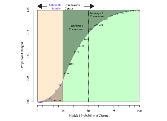
2.6. Accuracy Optimization Technique 1—Eliminating Commission
2.7. Accuracy Optimization Technique 2—Lowering the Change Candidate Threshold
2.8. Estimating Omission
2.9. Assessment of Accuracy Optimization
3. Results
3.1. Comparison of Four Different Change Outputs
| Model | Change Probability Threshold | Reviewed Change Polygons | Modeled Change Area (ha) | Removed Commission Area (ha) | Verified Change Area (ha) | Dissolved Change Locations |
|---|---|---|---|---|---|---|
| RF50/AO50 Map | ≥50% | 7832 | 3866 | 87 | 3779 | 2348 |
| RF25/AO25 Map | ≥25% | 16,524 | 5354 | 833 | 4521 | 5607 |
3.2. Random Forests Statistical Prediction of Land Cover Change in the Puyallup Watershed, 2006–2009
3.3. Commission Error Removal from the RF50 Land Cover Change Map
3.4. Omission Estimate for the RF50/AO50 Change Model

3.5. Commission Error Removal from the RF25 Land Cover Change Map
3.6. Omission Estimate for the RF25/AO25 Change Map
3.7. Accuracy Optimization Assessment

| Bins | Polygons | Hectares | Observed Polygons | Observed Hectares | Observed Change Polygons | Observed Change Hectares | Polygon Percent Change | Area Percent Change | Polygon Prediction | Hectares Prediction | Hours To Review |
|---|---|---|---|---|---|---|---|---|---|---|---|
| (0%–5%) | 343210 | 237400 | 4037 | 2705 | 9 | 1.1 | 0.2% | 0.04% | 765 | 94 | 1373 |
| (5%–10%) | 61783 | 15708 | 757 | 193 | 12 | 1.3 | 1.6% | 0.68% | 979 | 107 | 247 |
| (10%–15%) | 23090 | 5754 | 290 | 69 | 12 | 1.3 | 4.1% | 1.89% | 955 | 108 | 92 |
| (15%–20%) | 10645 | 2906 | 106 | 26 | 13 | 2.8 | 12.3% | 11.10% | 1306 | 322 | 43 |
| (20%–25%) | 5297 | 968 | 62 | 8 | 12 | 1.6 | 19.4% | 21.50% | 1025 | 208 | 21 |
4. Discussion
4.1. Improved Map Accuracy for Data Integration
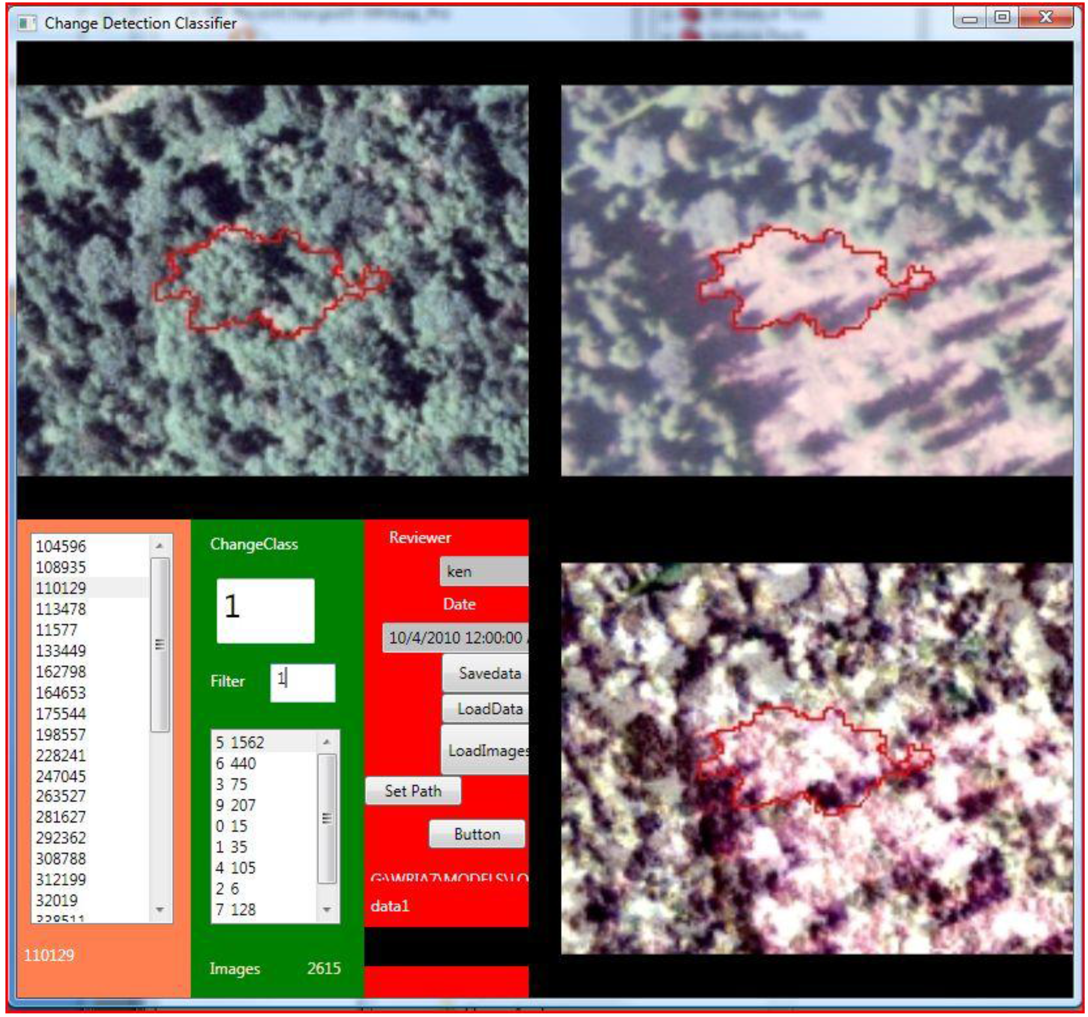
4.2. The AAClipGenerator/AAViewer System
5. Conclusions
- The combined accuracy optimization techniques improved the detection of urbanizing land-cover by increasing the mapped development-related change area by 93% in the AO25 map compared to the base map produced by the initial prediction model, the RF50 map and raised the total number of individual mapped change locations by 239% from 2348 to 5607 (Table 2).
- A total change estimate was generated by both “eliminating” commission and estimating omission. That estimate was comprised of 86.6% mapped change events and 13.4% estimated unmapped change.
- A software system was developed to assess training data locations and to determine classification accuracy that greatly reduced analyst review time allowing review of 1000s of accuracy assessment and training data locations in the time previously required to view 100s.
- Searching for additional change through threshold lowering is a powerful technique for optimizing change mapping when using a probabilistic classifier like RF and a system for rapidly checking predictions as developed here.
- The image data used in this analysis is available for many parts of the United States and the techniques described here are applicable to any object-based mapping exercise using imagery of high enough resolution to verify classifications through manual photo interpretation.
Acknowledgments
Conflicts of Interest
References and Notes
- Rindfuss, R.R.; Walsh, S.J.; Turner, B.L.; Fox, J.; Mishra, V. Developing a science of land change: Challenges and methodological issues. Proc. Natl. Acad. Sci. USA 2004, 101, 13976–13981. [Google Scholar] [CrossRef] [PubMed]
- Turner, B.; Lambin, E.F.; Reenberg, A. The emergence of land change science for global environmental change and sustainability. Proc. Natl. Acad. Sci. USA 2007, 104, 20666–20671. [Google Scholar] [CrossRef] [PubMed]
- Solecki, W.; Seto, K.C.; Marcotullio, P.J. It’s Time for an Urbanization Science. Environ. Sci. Policy Sustain. Dev. 2013, 55, 12–17. [Google Scholar] [CrossRef]
- Rogan, J.; Chen, D. Remote sensing technology for mapping and monitoring land-cover and land-use change. Prog. Plann. 2004, 61, 301–325. [Google Scholar] [CrossRef]
- Kennedy, R.E.; Townsend, P.A.; Gross, J.E.; Cohen, W.B.; Bolstad, P.; Wang, Y.Q.; Adams, P. Remote sensing change detection tools for natural resource managers: Understanding concepts and tradeoffs in the design of landscape monitoring projects. Remote Sens. Environ. 2009, 113, 1382–1396. [Google Scholar] [CrossRef]
- Petter, M.; Mooney, S.; Maynard, S.M.; Davidson, A.; Cox, M.; Horosak, I. A methodology to map ecosystem functions to support ecosystem services assessments. Ecol. Soc. 2013, 18, 31. [Google Scholar] [CrossRef]
- Thackway, R.; Lymburner, L.; Guerschman, J.P. Dynamic land cover information: Bridging the gap between remote sensing and natural resource management. Ecol. Soc. 2013, 18. [Google Scholar] [CrossRef]
- Goetz, S.J.; Wright, R.K.; Smith, A.J.; Zinecker, E.; Schaub, E. IKONOS imagery for resource management: Tree cover, impervious surfaces, and riparian buffer analyses in the mid-Atlantic region. Remote Sens. Environ. 2003, 88, 195–208. [Google Scholar] [CrossRef]
- Wulder, M.A.; Hall, R.J.; Coops, N.C.; Franklin, S.E. High Spatial Resolution Remotely Sensed Data for Ecosystem Characterization. Bioscience 2004, 54, 511–521. [Google Scholar] [CrossRef]
- Morgan, J.L.; Gergel, S.E.; Coops, N.C. Aerial photography: A rapidly evolving tool for ecological management. Bioscience 2010, 60, 47–59. [Google Scholar] [CrossRef]
- Lu, D.; Hetrick, S.; Moran, E. Impervious surface mapping with QuickBird imagery. Int. J. Remote Sens. 2011, 32, 2519–2533. [Google Scholar] [CrossRef] [PubMed]
- Johansen, K.; Roelfsema, C.; Phinn, S. SPECIAL FEATURE—High Spatial Resolution Remote Sensing for Environmental Monitoring and Management PREFACE:. J. Spat. Sci. 2008, 53, 43–48. [Google Scholar] [CrossRef]
- Myint, S.W.; Gober, P.; Brazel, A.; Grossman-Clarke, S.; Weng, Q. Per-pixel vs. object-based classification of urban land cover extraction using high spatial resolution imagery. Remote Sens. Environ. 2011, 115, 1145–1161. [Google Scholar] [CrossRef]
- Baker, B.A.; Warner, T.A.; Conley, J.F.; Mcneil, B.E. Does spatial resolution matter? A multi- scale comparison of object-based and pixel-based methods for detecting change associated with gas well drilling operations. Int. J. Remote Sens. Publ. 2012, 34, 37–41. [Google Scholar] [CrossRef]
- Chen, G.; Hay, G.J.; Carvalho, L.M.T.; Wulder, M.A. Object-based Change Detection. Int. J. Remote Sens. 2012, 33, 4434–4457. [Google Scholar] [CrossRef]
- Desclée, B.; Bogaert, P.; Defourny, P. Forest change detection by statistical object-based method. Remote Sens. Environ. 2006, 102, 1–11. [Google Scholar] [CrossRef]
- Zhou, W.; Troy, A. An object-oriented approach for analysing and characterizing urban landscape at the parcel level. Int. J. Remote Sens. 2008, 29, 3119–3135. [Google Scholar] [CrossRef]
- Blaschke, T.; Lang, S.; Hay, G.J. Object-Based Image Analysis: Spatial Concepts for Knowledge-Driven Remote Sensing Applications; Lecture Notes in Geoinformation and Cartography; Springer-Verlag: Berlin/Heidelberg, Germany, 2008. [Google Scholar]
- Morgan, J.; Gergel, S. Automated analysis of aerial photographs and potential for historic forest mapping. Can. J. For. Res. 2013, 43, 699–710. [Google Scholar]
- Lillesand, T.; Kiefer, R.W.; Chipman, J. Remote Sensing and Image Interpretation; John Wiley Sons Inc.: New York, NY, USA, 2003. [Google Scholar]
- Du, P.; Liu, P.; Xia, J.; Feng, L.; Liu, S.; Tan, K.; Cheng, L. Remote sensing image interpretation for urban environment analysis: methods, system and examples. Remote Sens. 2014, 6, 9458–9474. [Google Scholar] [CrossRef]
- Jelinski, D.E.; Wu, J. The modifiable areal unit problem and implications for landscape ecology. Landsc. Ecol. 1996, 11, 129–140. [Google Scholar] [CrossRef]
- Linke, J.; McDermid, G.J.; Pape, A.D.; McLane, A.J.; Laskin, D.N.; Hall-Beyer, M.; Franklin, S.E. The influence of patch-delineation mismatches on multi-temporal landscape pattern analysis. Landsc. Ecol. 2008, 24, 157–170. [Google Scholar] [CrossRef]
- Karl, J.W.; Maurer, B.A. Multivariate correlations between imagery and field measurements across scales: comparing pixel aggregation and image segmentation. Landsc. Ecol. 2009, 25, 591–605. [Google Scholar] [CrossRef]
- Aubrecht, C.; Steinnocher, K.; Hollaus, M.; Wagner, W. Integrating earth observation and GIScience for high resolution spatial and functional modeling of urban land use. Comput. Environ. Urban Syst. 2009, 33, 15–25. [Google Scholar] [CrossRef]
- Johansen, K.; Phinn, S.; Witte, C. Mapping of riparian zone attributes using discrete return LiDAR, QuickBird and SPOT-5 imagery: Assessing accuracy and costs. Remote Sens. Environ. 2010, 114, 2679–2691. [Google Scholar] [CrossRef]
- O’Neil-Dunne, J.; MacFaden, S.; Royar, A. A versatile, production-oriented approach to high-resolution tree-canopy mapping in urban and suburban landscapes using GEOBIA and data fusion. Remote Sens. 2014, 6, 12837–12865. [Google Scholar] [CrossRef]
- Hong, B.; Limburg, K.E.; Hall, M.H.; Mountrakis, G.; Groffman, P.M.; Hyde, K.; Luo, L.; Kelly, V.R.; Myers, S.J. An integrated monitoring/modeling framework for assessing human–nature interactions in urbanizing watersheds: Wappinger and Onondaga Creek watersheds, New York, USA. Environ. Model. Softw. 2012, 32, 1–15. [Google Scholar] [CrossRef]
- Levin, S.A.; Dec, N. The problem of pattern and scale in ecology: The Robert H. MacArthur Award Lecture. Ecology 1992, 73, 1943–1967. [Google Scholar] [CrossRef]
- Wu, H.; Li, Z.-L. Scale issues in remote sensing: A review on analysis, processing and modeling. Sensors 2009, 9, 1768–1793. [Google Scholar] [CrossRef] [PubMed]
- Burnicki, A.C. Impact of error on landscape pattern analyses performed on land-cover change maps. Landsc. Ecol. 2012, 27, 713–729. [Google Scholar] [CrossRef]
- Stehman, S.V.; Wickham, J.D. Assessing accuracy of net change derived from land cover maps. Photogramm. Eng. Remote Sens. 2006, 72, 175–185. [Google Scholar] [CrossRef]
- Walter, V. Object-based classification of remote sensing data for change detection. ISPRS J. Photogramm. Remote Sens. 2004, 58, 225–238. [Google Scholar] [CrossRef]
- Burnett, C.; Blaschke, T. A multi-scale segmentation/object relationship modelling methodology for landscape analysis. Ecol. Model. 2003, 168, 233–249. [Google Scholar] [CrossRef]
- Blaschke, T. Object based image analysis for remote sensing. ISPRS J. Photogramm. Remote Sens. 2010, 65, 2–16. [Google Scholar] [CrossRef]
- Congalton, R.G.; Green, K. Assessing the Accuracy of Remotely Sensed Data: Principles and Practices, Second Edition (Mapping Science); CRC Press: Boca Raton, FL, USA, 2008. [Google Scholar]
- Fawcett, T. An introduction to ROC analysis. Pattern Recognit. Lett. 2006, 27, 861–874. [Google Scholar] [CrossRef]
- Lu, D.; Weng, Q. A survey of image classification methods and techniques for improving classification performance. Int. J. Remote Sens. 2007, 28, 823–870. [Google Scholar] [CrossRef]
- Strahler, A.H.; Woodcock, C.E.; Smith, J.A. On the nature of models in remote sensing. Remote Sens. Environ. 1986, 20, 121–139. [Google Scholar] [CrossRef]
- Woodcock, C.E.; Strahler, A.H. The factor of scale in remote sensing. Remote Sens. Environ. 1987, 21, 311–332. [Google Scholar] [CrossRef]
- Haralick, R.M.; Shapiro, L.G. Image segmentation techniques. Comput. Vis. Graph. Image Process. 1985, 29, 100–132. [Google Scholar] [CrossRef]
- Hay, G.J.; Castilla, G.; Wulder, M.A.; Ruiz, J.R. An automated object-based approach for the multiscale image segmentation of forest scenes. Int. J. Appl. Earth Obs. Geoinf. 2005, 7, 339–359. [Google Scholar] [CrossRef]
- Lu, D.; Mausel, P.; Brondízio, E.; Moran, E. Change detection techniques. Int. J. Remote Sens. 2004, 25, 2365–2401. [Google Scholar] [CrossRef]
- Weng, Q. Remote sensing of impervious surfaces in the urban areas: Requirements, methods, and trends. Remote Sens. Environ. 2012, 117, 34–49. [Google Scholar] [CrossRef]
- Singh, A. Digital change detection techniques using remotely-sensed data. Int. J. Remote Sens. 1989, 10, 989–1003. [Google Scholar] [CrossRef]
- Coppin, P.; Jonckheere, I.; Nackaerts, K.; Muys, B.; Lambin, E. Digital change detection methods in ecosystem monitoring: A review. Int. J. Remote Sens. 2004, 25, 1565–1596. [Google Scholar] [CrossRef]
- Linke, J.; Mcdermid, G.J.; Laskin, D.N.; Mclane, A.J.; Pape, A.; Cranston, J.; Franklin, S.E. A disturbance-inventory framework for flexible and reliable landscape monitoring. Photogramm. Eng. Remote Sens. 2009, 75, 981–995. [Google Scholar] [CrossRef]
- Im, J.; Jensen, J.R.; Tullis, J.A. Object-based change detection using correlation image analysis and image segmentation. Int. J. Remote Sens. 2008, 29, 399–423. [Google Scholar] [CrossRef]
- Foody, G.M. Status of land cover classification accuracy assessment. Remote Sens. Environ. 2002, 80, 185–201. [Google Scholar] [CrossRef]
- Nusser, S.; Klaas, E. Survey methods for assessing land cover map accuracy. Environ. Ecol. Stat. 2003, 10, 309–331. [Google Scholar] [CrossRef]
- Edwards, T.; Moisen, G.; Cutler, D. Assessing map accuracy in a remotely sensed, ecoregion-scale cover map. Remote Sens. Environ. 1998, 63, 73–83. [Google Scholar] [CrossRef]
- Stehman, S.; Czaplewski, R. Design and analysis for thematic map accuracy assessment: Fundamental principles. Remote Sens. Environ. 1998, 344, 331–344. [Google Scholar] [CrossRef]
- Hastie, T.; Tibshirani, R.; Friedman, J. The Elements of Statistical Learning: Data Mining, Inference, and Prediction, Second Edition (Springer Series in Statistics); Springer: New York, NY, USA, 2009. [Google Scholar]
- Aleksandrowicz, S.; Turlej, K.; Lewiński, S.; Bochenek, Z. Change detection algorithm for the production of land cover change maps over the European Union countries. Remote Sens. 2014, 6, 5976–5994. [Google Scholar] [CrossRef]
- Hepinstall-Cymerman, J.; Coe, S.; Hutyra, L.R. Urban growth patterns and growth management boundaries in the Central Puget Sound, Washington, 1986–2007. Urban Ecosyst. 2013, 16, 109–129. [Google Scholar] [CrossRef]
- Gray, A.N.; Azuma, D.L.; Lettman, G.J.; Thompson, J.L.; McKay, N. Changes in Land Use and Housing on Resource Lands in Washington State, 1976–2006; USDA PNW Research Station: Washington, DC, USA, 2013.
- Pontius, R.G.; Shusas, E.; McEachern, M. Detecting important categorical land changes while accounting for persistence. Agric. Ecosyst. Environ. 2004, 101, 251–268. [Google Scholar] [CrossRef]
- Olofsson, P.; Foody, G.M.; Stehman, S.V.; Woodcock, C.E. Making better use of accuracy data in land change studies: Estimating accuracy and area and quantifying uncertainty using stratified estimation. Remote Sens. Environ. 2013, 129, 122–131. [Google Scholar] [CrossRef]
- Liknes, G.; Perry, C.; Meneguzzo, D. Assessing tree cover in agricultural landscapes using high-resolution aerial imagery. J. Terr. Obs. 2010, 2, 38–55. [Google Scholar]
- Claggett, P.R.; Okay, J.A.; Stehman, S.V. Monitoring regional Riparian forest cover change using stratified sampling and multiresolution imagery. J. Am. Water Resour. Assoc. 2010, 46, 334–343. [Google Scholar] [CrossRef]
- Moskal, L.M.; Styers, D.M.; Halabisky, M. Monitoring urban tree cover using object-based image analysis and public domain remotely sensed data. Remote Sens. 2011, 3, 2243–2262. [Google Scholar] [CrossRef]
- Li, X.; Shao, G. Object-based land-cover mapping with high resolution aerial photography at a county scale in midwestern USA. Remote Sens. 2014, 6, 11372–11390. [Google Scholar] [CrossRef]
- Yuan, F. Land cover change and environmental impact analysis in the Greater Mankato area of Minnesota using remote sensing and GIS modelling. Int. J. Remote Sens. 2008, 29, 1169–1184. [Google Scholar] [CrossRef]
- Goward, S.N.; Davis, P.E.; Fleming, D.; Miller, L.; Townshend, J.R. Empirical comparison of Landsat 7 and IKONOS multispectral measurements for selected Earth Observation System (EOS) validation sites. Remote Sens. Environ. 2003, 88, 80–99. [Google Scholar] [CrossRef]
- Ehlers, M.; Gaehler, M.; Janowsky, R. Automated techniques for environmental monitoring and change analyses for ultra high-resolution remote sensing data. Photogramm. Eng. Remote Sens. 2006, 7, 835–844. [Google Scholar] [CrossRef]
- Lu, D.; Hetrick, S.; Moran, E.; Li, G. Detection of urban expansion in an urban-rural landscape with multitemporal QuickBird images. J. Appl. Remote Sens. 2010, 4, 1–22. [Google Scholar]
- Dare, P. Shadow analysis in high-resolution satellite imagery of urban areas. Photogramm. Eng. Remote Sens. 2005, 71, 169–177. [Google Scholar] [CrossRef]
- Cleve, C.; Kelly, M.; Kearns, F.R.; Moritz, M. Classification of the wildland–urban interface: A comparison of pixel- and object-based classifications using high-resolution aerial photography. Comput. Environ. Urban Syst. 2008, 32, 317–326. [Google Scholar] [CrossRef]
- Zhou, W.; Troy, A.; Grove, M. Object-based land cover classification and change analysis in the Baltimore metropolitan area using multitemporal high resolution remote sensing data. Sensors 2008, 8, 1613–1636. [Google Scholar] [CrossRef]
- Cadenasso, M.L.; Pickett, S.T.A.; Schwarz, K. Spatial heterogeneity in urban ecosystems: Reconceptualizing land cover and a framework for classification. Front. Ecol. Environ. 2007, 5, 80–88. [Google Scholar] [CrossRef]
- Trimble eCognition Developer 8.7.2, 2012; 262.
- Linke, J.; McDermid, G.J. A conceptual model for multi-temporal landscape monitoring in an object-based environment. IEEE J. Sel. Top. Appl. Earth Obs. Remote Sens. 2011, 4, 265–271. [Google Scholar] [CrossRef]
- Haralick, R.; Shanmugan, K.; Dinstein, I. Textural features for image classification. IEEE Trans. Syst. Man Cybern. 1973, 3, 610–621. [Google Scholar] [CrossRef]
- Huth, J.; Kuenzer, C.; Wehrmann, T.; Gebhardt, S.; Tuan, V.Q.; Dech, S. Land cover and land use classification with TWOPAC: Towards automated processing for pixel- and object-based image classification. Remote Sens. 2012, 4, 2530–2553. [Google Scholar] [CrossRef]
- ESRI (Environmental Systems Resource Institute) ArcMap 10.1, 2011.
- Breiman, L. Random Forests. Mach. Learn. 2001, 45, 5–32. [Google Scholar] [CrossRef]
- Cutler, D.R.; Edwards, T.C.; Beard, K.H.; Cutler, A.; Hess, K.T.; Gibson, J.; Lawler, J.J. Random forests for classification in ecology. Ecology 2007, 88, 2783–2792. [Google Scholar] [CrossRef] [PubMed]
- Timm, B.; McGarigal, K. Fine-scale remotely-sensed cover mapping of coastal dune and salt marsh ecosystems at Cape Cod National Seashore using Random Forests. Remote Sens. Environ. 2012, 127, 106–117. [Google Scholar] [CrossRef]
- R Core Team. R: A Language and Environment for Statistical Computing; R Foundation for Statistical Computing: Vienna, Austria, 2013. [Google Scholar]
- Liaw, A.; Wiener, M. Classification and regression by randomForest. R News 2002, 2, 18–22. [Google Scholar]
- Guisan, A.; Zimmermann, N.E. Predictive habitat distribution models in ecology. Ecol. Modell. 2000, 135, 147–186. [Google Scholar] [CrossRef]
- Moisen, G.G.; Frescino, T.S. Comparing five modelling techniques for predicting forest characteristics. Ecol. Modell. 2002, 157, 209–225. [Google Scholar] [CrossRef]
- Zimmerman, P.L.; Housman, I.W.; Perry, C.H.; Chastain, R.A.; Webb, J.B.; Finco, M.V. An accuracy assessment of forest disturbance mapping in the western Great Lakes. Remote Sens. Environ. 2013, 128, 176–185. [Google Scholar] [CrossRef]
- Gregory, R.; Failing, L.; Harstone, M.; Long, G.; McDaniels, T.; Ohlson, D. Structured Decision Making: A Practical Guide to Environmental Management Choices; Wiley-Blackwell: West Sussex, UK, 2012. [Google Scholar]
- Antrop, M. Landscape change and the urbanization process in Europe. Landsc. Urban Plan. 2004, 67, 9–26. [Google Scholar] [CrossRef]
- Jensen, K.C. An Evaluation of Land Cover Change from 2006 to 2009 and the Effectiveness of Certain Conservation Land Use Tools Within Lake Washington/Cedar/Sammamish Watershed (WRIA 8) Riparian Buffers. Master’ Thesis, University of Washington, Washington, DC, USA, 2012. [Google Scholar]
- ERDAS Imagine 2010 Field Guide TM, 2010; 842p.
© 2015 by the authors; licensee MDPI, Basel, Switzerland. This article is an open access article distributed under the terms and conditions of the Creative Commons Attribution license (http://creativecommons.org/licenses/by/4.0/).
Share and Cite
Pierce, K.B., Jr. Accuracy Optimization for High Resolution Object-Based Change Detection: An Example Mapping Regional Urbanization with 1-m Aerial Imagery. Remote Sens. 2015, 7, 12654-12679. https://doi.org/10.3390/rs71012654
Pierce KB Jr. Accuracy Optimization for High Resolution Object-Based Change Detection: An Example Mapping Regional Urbanization with 1-m Aerial Imagery. Remote Sensing. 2015; 7(10):12654-12679. https://doi.org/10.3390/rs71012654
Chicago/Turabian StylePierce, Kenneth B., Jr. 2015. "Accuracy Optimization for High Resolution Object-Based Change Detection: An Example Mapping Regional Urbanization with 1-m Aerial Imagery" Remote Sensing 7, no. 10: 12654-12679. https://doi.org/10.3390/rs71012654