Validation of Long-Term Global Aerosol Climatology Project Optical Thickness Retrievals Using AERONET and MODIS Data

Abstract

A comprehensive set of monthly mean aerosol optical thickness (AOT) data from coastal and island AErosol RObotic NETwork (AERONET) stations is used to evaluate Global Aerosol Climatology Project (GACP) retrievals for the period 1995–2009 during which contemporaneous GACP and AERONET data were available. To put the GACP performance in broader perspective, we also compare AERONET and MODerate resolution Imaging Spectroradiometer (MODIS) Aqua level-2 data for 2003–2009 using the same methodology. We find that a large mismatch in geographic coverage exists between the satellite and ground-based datasets, with very limited AERONET coverage of open-ocean areas. This is especially true of GACP because of the smaller number of AERONET stations at the early stages of the network development. Monthly mean AOTs from the two over-the-ocean satellite datasets are well-correlated with the ground-based values, the correlation coefficients being 0.81–0.85 for GACP and 0.74–0.79 for MODIS. Regression analyses demonstrate that the GACP mean AOTs are approximately 17%–27% lower than the AERONET values on average, while the MODIS mean AOTs are 5%–25% higher. The regression coefficients are highly dependent on the weighting assumptions (e.g., on the measure of aerosol variability) as well as on the set of AERONET stations used for comparison. Comparison of over-the-land and over-the-ocean MODIS monthly mean AOTs in the vicinity of coastal AERONET stations reveals a significant bias. This may indicate that aerosol amounts in coastal locations can differ significantly from those in adjacent open-ocean areas. Furthermore, the color of coastal waters and peculiarities of coastline meteorological conditions may introduce biases in the GACP AOT retrievals. We conclude that the GACP and MODIS over-the-ocean retrieval algorithms show similar ranges of discrepancy when compared to available coastal and island AERONET stations. The factors mentioned above may limit the performance of the validation procedure and cause us to caution against a direct extrapolation of the presented validation results to the entirety of the GACP dataset.

1. Introduction

Current uncertainties in our knowledge of the aerosol radiative effects cause substantial limitations on the accuracy of global circulation model predictions of climate change [1,2,3,4,5]. Owing to their near-global and quasi-uniform coverage, satellite-based retrievals of aerosol properties may help improve the robustness of climate modeling by providing constrains on the global distribution of aerosols.

The main product of the Global Aerosol Climatology Project (GACP, [6]) is one of the longest aerosol optical thickness (AOT) datasets covering the period between August 1983 and December 2009. This product is based on the gridded and cloud-screened International Satellite Cloud Climatology Project (ISCCP) DX radiances [7] obtained by sub-sampling to 30 × 30 km the Advanced Very High Resolution Radiometer Global Area Coverage (AVHRR GAC) data from a succession of National Oceanic and Atmospheric (NOAA) weather satellites. Using the GACP product, Mishchenko et al. [8] identified a likely downward trend in the global tropospheric AOT over the oceans during the period from the late 1980s to the early 2000s, consistent with the contemporaneous switch from global dimming to global brightening [9]. Mishchenko and Geogdzhayev [10] identified regional decreases of tropospheric aerosol amounts over much of Europe and a significant part of the Atlantic Ocean as well as upward AOT trends over long stretches of African and Asian coasts. These results were confirmed by Zhao et al. [11] and are consistent, at least qualitatively, with extensive ground-based observations [12] and available emission-inventory assessments [13,14]. Furthermore, Yoon et al. [15] used data from multiple instruments to identify a statistically significant AOT decrease over Europe and an increase over China between 2003 and 2008, again in agreement with the GACP results. Most recently, Geogdzhayev et al. [16] combined the data from morning and afternoon AVHRR instruments to extend the GACP record through the end of 2009. They found that the downward AOT trend ended by the early 2000s and was replaced by flat (on average) AOT values, in line with the contemporaneous MODIS and MISR AOT results [17,18].

Given the important role that the aerosols play in climate change, considerable efforts have been made to validate satellite data products. Typically, validation involves a combination of several approaches such as comparisons with ground-based data, consistency checks, and intercomparisons of satellite datasets, all of which, taken together, are intended to yield quantitative estimates of the retrieval accuracy and stability. For example, Liu et al. [19] evaluated the GACP AOT retrievals using ensemble-averaged ship-borne sun-photometer results collected during the period 1986–1996. They found a strong correlation between the satellite results and the ship measurements, while being forced to introduce an adjustment to the diffuse component of the ocean surface reflectance in the GACP retrieval algorithm to produce a better match. A similar study was performed by Smirnov et al. [20].

The expansion of the ground-based AErosol RObotic NETwork over the last two decades (AERONET; [21,22]) has resulted in a growing number of coastal and island stations providing extended AOT time-series. This makes it possible to attempt a thorough validation of the over-the-ocean GACP AOT retrievals, including the more recent segment of the GACP record. Accordingly, the main goal of this study is to perform a systematic global comparison of the GACP AOTs to the suitable AERONET measurements.

Furthermore, since the early 2000s, global AOT data from newer and more advanced satellite instruments such as the Moderate Resolution Imaging Spectroradiometer (MODIS, [23,24,25]) have been available. Therefore, in this study we also use MODIS data as a contextual benchmark for evaluating the robustness of the GACP-AERONET comparison. The MODIS dataset appears to be an especially suitable choice for this study because the MODIS AOT data have been thoroughly characterized (e.g., [25,26,27,28,29,30,31,32]), including by comparing them with AERONET measurements, and have been widely used in aerosol research. In particular, Remer et al. [28] compared two years of AERONET data with collocated MODIS AOTs and estimated that two-thirds of MODIS-derived AOTs should fall within the ±0.03 ± 0.05 τ_AERONET envelope over the oceans.

There are two factors making direct pixel-level GACP-AERONET comparisons less straightforward and definitive than they would be in an ideal setting. The first one is the limited capability of a two-channel satellite retrieval algorithm in which all model parameters but two must be globally fixed. Among these globally-fixed parameters are the aerosol refractive index, morphology, and vertical distribution, as well as the type of the particle size distribution [33]. The second factor is the poor data density of the GACP retrievals. Because of the limited performance of the satellite algorithm, our validation strategy is to compare AOT averages taken over an extended period of time (e.g., a month) and over a relatively large area around an AERONET station. As mentioned above, to provide a context for the GACP-AERONET comparisons we also perform MODIS-AERONET comparisons using the same basic strategy.

2. Data

The nominal GACP dataset is documented in [10,16,33,34] and can be obtained from http://gacp.giss.nasa.gov. As already mentioned, it is based on analyzing channel one (0.65 μm) and channel two (0.85 μm) radiance data from the AVHRR instruments on-board NOAA satellites over the oceans provided by the ISCCP DX dataset [7]. The GACP retrieval algorithm yields the column-integrated AOT and column-averaged Ångström exponent (AE) for each cloud-free ISCCP DX pixel by minimizing the difference between the AVHRR radiances for the instantaneous illumination and observation angles defined by the satellite orbit and the radiances simulated theoretically for a realistic atmosphere-ocean radiative transfer model [33].

AERONET level 2.0 AOT data used in this study were downloaded from aeronet.gsfc.nasa.gov. All stations were mapped onto a 0.5° × 0.5° land/ocean mask. Since we are interested in coastal and island AOT measurements, only stations surrounded by more than three ocean mask cells were retained. AOT values at 550 nm were then found by interpolation using the 500 nm AOT in combination with the 440–870 nm AE. If AOT values at 500 nm were not available, the values at 675 nm were used instead. These interpolated AOT values were used to calculate the monthly means. To create a more consistent dataset for comparison with satellite data, we required that at least 75 measurements from at least 15 days in a given month were present. The reason for this restriction is to avoid data points where reliable estimation of monthly mean values was not possible due to the measurements interruptions or persisting overcast cloudiness.

A number of problems complicate the comparison of AERONET and satellite-derived AOTs. Among them are temporal and spatial collocation difficulties and differences in cloud screening. A number of strategies may be adopted to deal with these problems (e.g., [31]). One commonly-used approach is to collocate ground-based and satellite AOT measurements and to compare the temporal mean ground-based AOT with the spatially-averaged satellite-derived value within the collocation window. In this approach the satellite observation geometry, and the atmospheric and surface conditions are fixed for each comparison point, thereby facilitating the analysis of the retrieval algorithm performance. The disadvantage of this approach is that the situations wherein only the satellite or only the ground-based measurement is available are excluded, thus making the evaluation potentially incomplete. Another approach is to compare spatially-collocated averages over a sufficiently long period (e.g., a month). In this way all available satellite and ground-based data are included in the averages, making the comparison more climatologically representative. On the other hand, the evaluation of the retrieval algorithm becomes more complicated since data pertaining to multiple observation geometries and atmospheric conditions contribute to the calculation of the means. Thus the two approaches are complementary, and one may be preferred over the other depending on the specific purpose of the analysis.

In this study, instead of comparing instantaneous AOT values, we compare monthly mean AOTs derived from AERONET and satellite data. One of the reasons for doing that is that the limited data density of the GACP dataset make direct point-to-point comparisons problematic. Note that among other factors, the two approaches differ in how cloud screening is treated. Instantaneous collocated AOT values are usually compared for scenes that are judged cloud free by both the ground-based and the satellite cloud screening algorithm. In the case of monthly AOT averages, cloud-screening decisions are implicitly included in the values being compared and may be the source of additional discrepancies.

To create a matching set of monthly retrievals, we aggregate GACP measurements, for each month and each AERONET station, within a 200 km circle centered on the geographic coordinates of the station. We require at least 15 retrievals to contribute to the monthly mean. In addition we require the standard deviation of the matching AERONET and GACP points not to exceed 70% of the monthly mean. The purpose of this restriction is to exclude unstable situations wherein ground-based and satellite monthly means may show a large discrepancy because of temporally- or spatially-variable transient events such as desert-dust or biomass-burning aerosol plumes.

To evaluate the GACP-AERONET comparison, we also performed a similar analysis using the MODIS dataset. We used Aqua Collection 5.1 Level 2 data for the period 2003–2009, downloaded from the Atmosphere Archive and Distribution System (LAADS) at ladsweb.nascom.nasa.gov.

3. GACP-AERONET Comparison

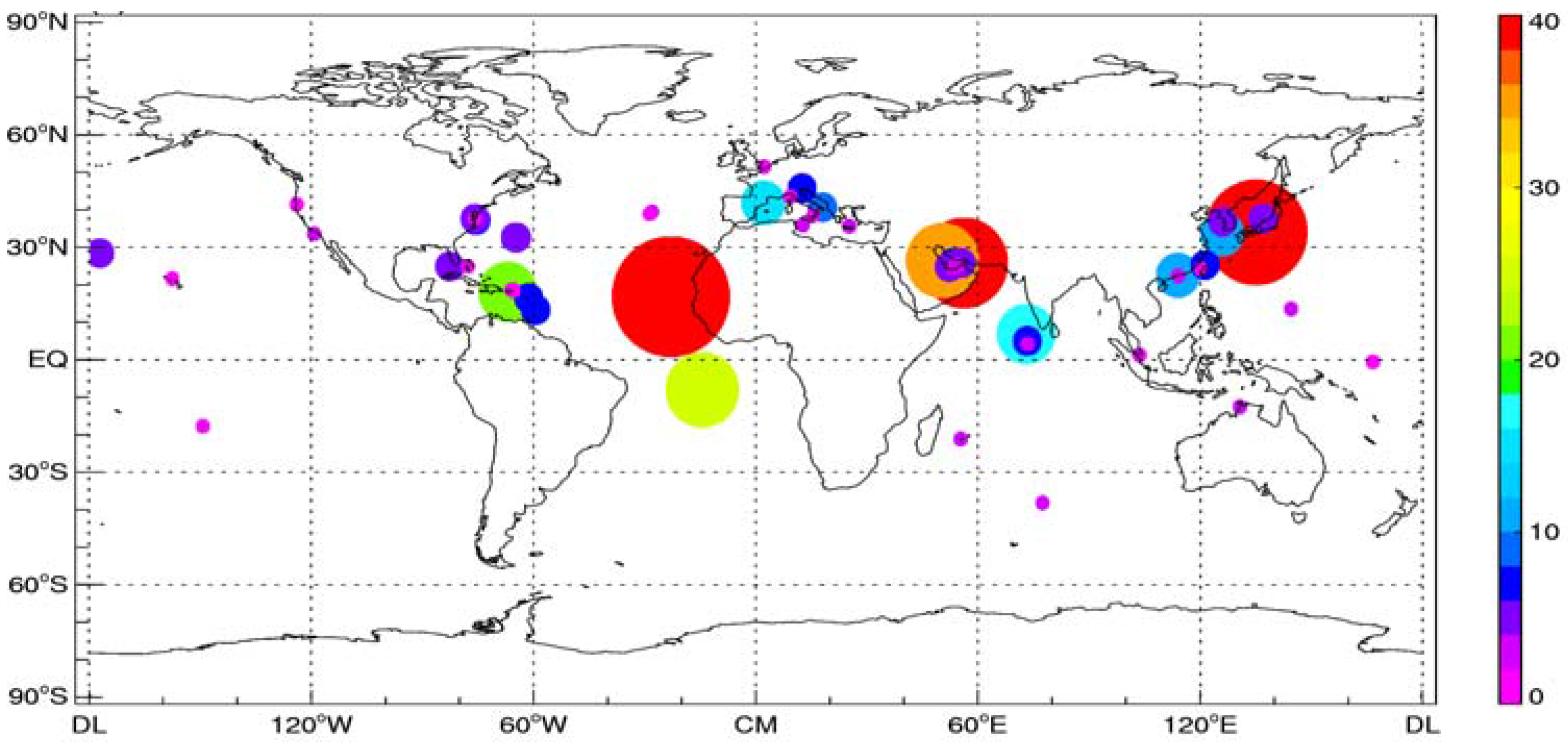
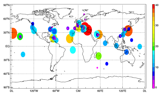
The geographical distribution of the GACP-AERONET matches is shown in Figure 1. Each AERONET station is shown by a colored circle centered on the geographic coordinates of the station. The area of each circle is proportional to the number of months for which a match was found. This number is also color-coded according to the color bar on the right-hand side. It is obvious from the figure that a large mismatch exists between the geographic coverage of the GACP and AERONET. The majority of the matches come from fewer than a dozen stations located in the Northern Hemisphere below the 40° latitude. With the exception of the Ascension Island station data in the Atlantic Ocean, the Southern Hemisphere is poorly represented in the dataset. Excluding the South-Eastern Asia region, only a few matches exist for the entire Pacific Ocean. Furthermore, while the majority of GACP data come from the open ocean areas, coastal AERONET stations are often located in areas close to aerosol sources such as the Saharan dust outflow region in the Atlantic Ocean, the Persian Gulf, or Southeast Asia.

Figure 1. Geographical distribution of GACP-AERONET matches. Each circle represents one AERONET station. The number of matches is quantified by the area of the corresponding circle and is also color-coded according to the bar on the right-hand side.

Figure 1. Geographical distribution of GACP-AERONET matches. Each circle represents one AERONET station. The number of matches is quantified by the area of the corresponding circle and is also color-coded according to the bar on the right-hand side.

The reason for this mismatch is twofold. First of all, the AERONET locations are optimized for the study of regions representative in terms of dominant aerosol types and the importance of the aerosol sources. The AERONET stations are also more densely spaced over land. On the other hand, the GACP coverage is over the water bodies only and otherwise is roughly uniform.

Second, the data density of the GACP set may not always be sufficient to reliably estimate the aerosol load in the vicinity of an AERONET station. This is especially true of coastal stations where much of the surrounding area may be land with no aerosol retrievals available.

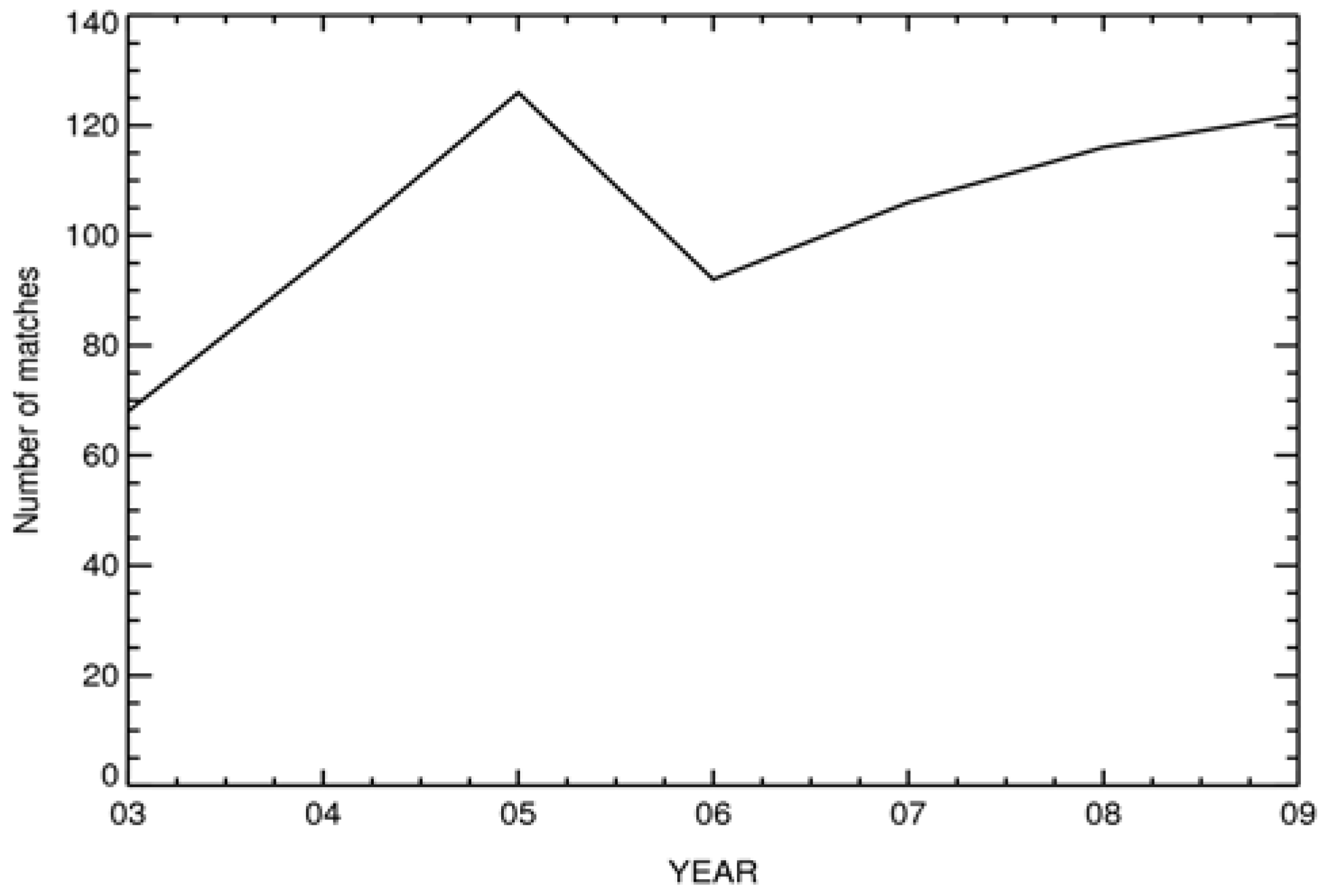
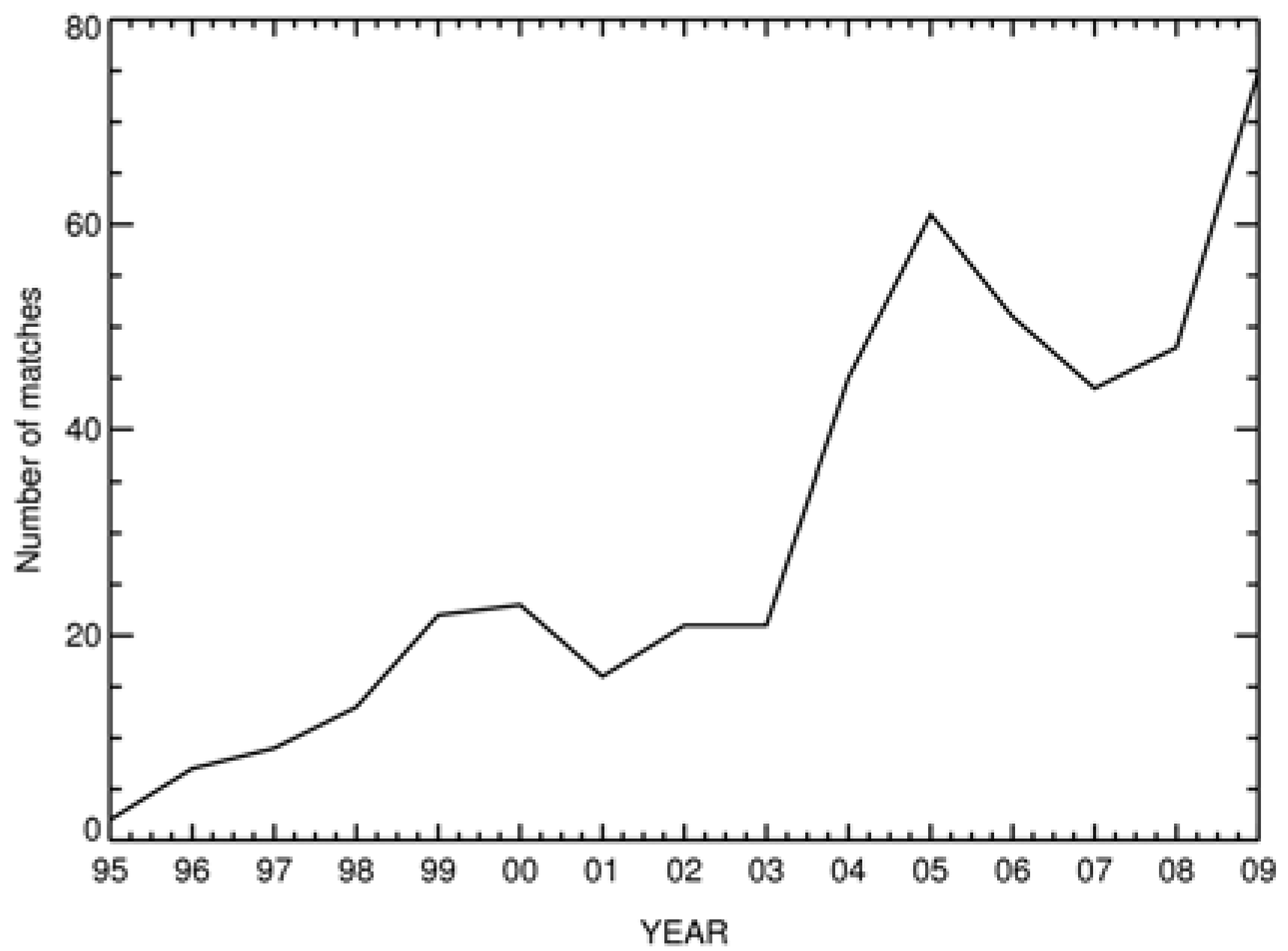
Figure 2 shows the cumulative yearly number of GACP-AERONET matches. One can see that the earliest year when matches became available was 1995 and that overall the number of matches has been increasing over time, reaching over 70 in 2009, the last year for which GACP data is currently available. The number of matches reflects the progress in the development of the AERONET network, as more stations went operational, but also the satellite-to-satellite transitions in the GACP record. For example, the dip in the number of matches in 2001 is associated with the data quality deterioration and the orbital drift at the end of life of NOAA-11, while the increase after 2003 may partly be due to the increased data density which resulted from the addition of the morning NOAA-17 AVHRR data to the afternoon NOAA-16 and NOAA-18 [16].

Figure 2. Time series of the number of GACP-AERONET monthly matches.

Figure 2. Time series of the number of GACP-AERONET monthly matches.

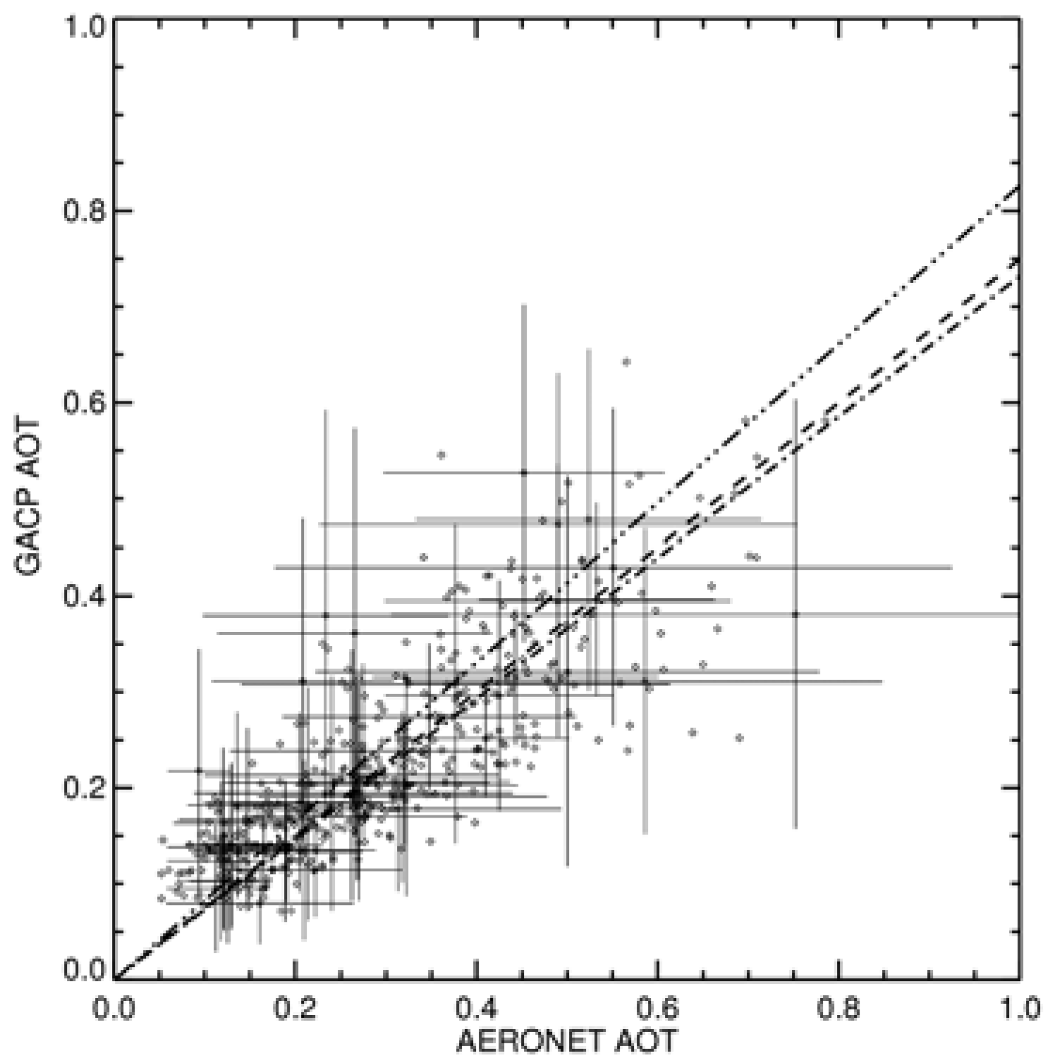
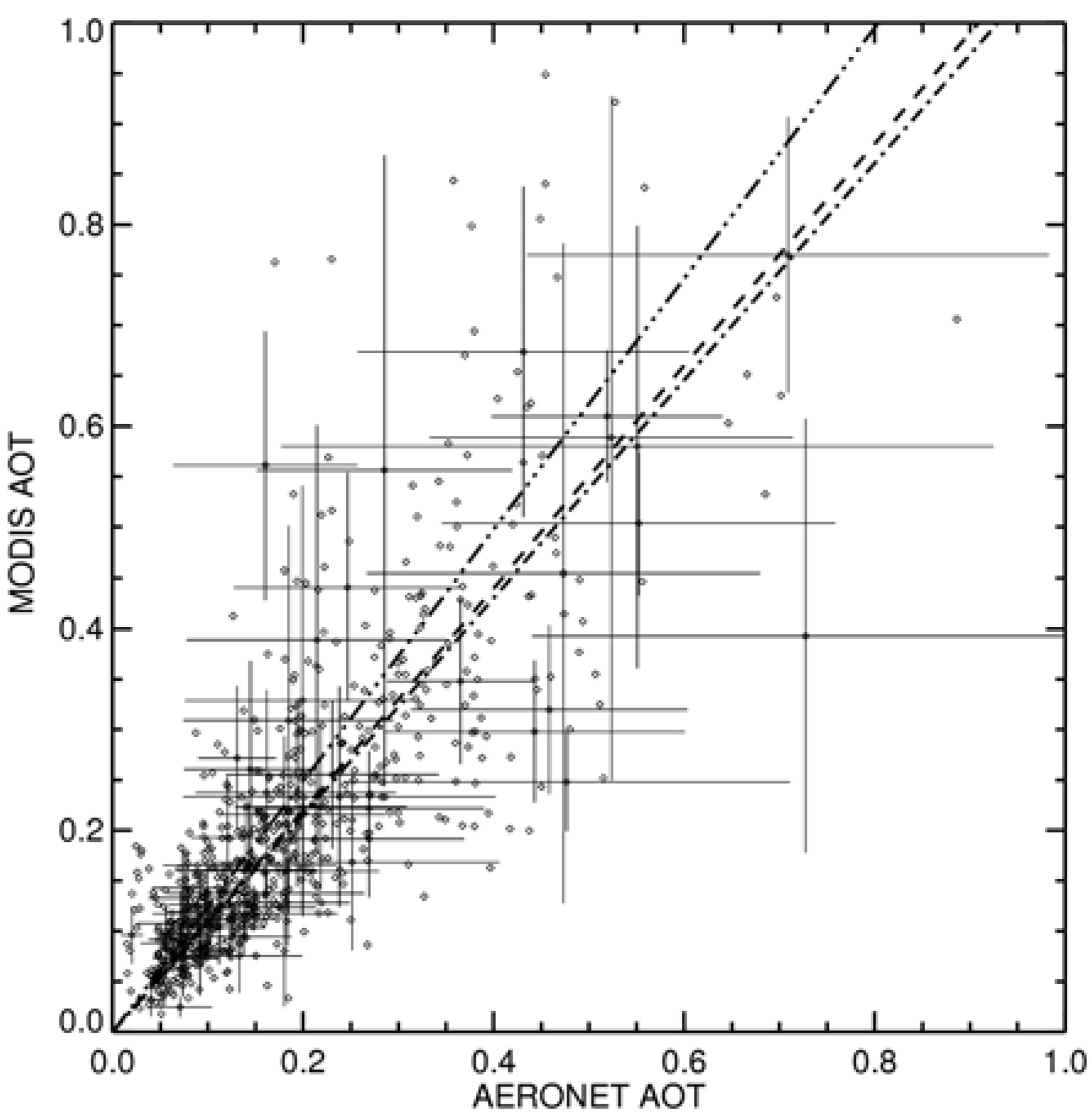
Figure 3 is a scatter plot of GACP vs. AERONET monthly mean AOT values. The relationship is characterized by a high correlation coefficient of 0.81 (here and below we use the sample Pearson correlation coefficient, defined as the ratio of the sample estimate of the covariance of two data vectors to the product of their standard deviations). Every matching point can be characterized by the standard deviation σ of the AOT values contributing to the monthly mean. These standard deviation values can be calculated from the AERONET or satellite data and are shown in Figure 3 by horizontal and vertical lines, respectively, for selected points to avoid clutter. Note that the lines are not error bars but rather represent natural aerosol variability in the vicinity of a particular station during a particular month.

Figure 3. Monthly GACP AOT vs. monthly AERONET AOT. The horizontal and vertical bars show one standard deviation of the selected AERONET and GACP values, respectively. Also shown are regression lines of the form y = ax for the uniform weighting (dot-dashed line, a = 0.73), for weighting with the AERONET σ (triple dot-dashed line, a = 0.83), and for weighting with the combined AERONET–GACP σ (dashed line, a = 0.75). The correlation coefficient is 0.81.

Figure 3. Monthly GACP AOT vs. monthly AERONET AOT. The horizontal and vertical bars show one standard deviation of the selected AERONET and GACP values, respectively. Also shown are regression lines of the form y = ax for the uniform weighting (dot-dashed line, a = 0.73), for weighting with the AERONET σ (triple dot-dashed line, a = 0.83), and for weighting with the combined AERONET–GACP σ (dashed line, a = 0.75). The correlation coefficient is 0.81.

The coefficients of linear regression of the GACP and AERONET datasets shown in Figure 3 potentially depend on the weights assigned to each point. The weighing has an implicit and an explicit component. The former is imposed by the composition of the comparison datasets and is affected, for example, by the geographical distribution of the AERONET stations or by the availability of satellite retrievals under various conditions. The latter is associated with the weighting of points once the comparison dataset is defined. There are several choices one can make. One can ignore the information on variability contained in the standard deviation σ, thereby ensuring the uniform weighting. Alternatively, it is reasonable to expect that, in general, monthly mean values for places with higher variability will be known with less accuracy and use the multiplicative inverses of the standard deviation as weights for calculating the linear regression between the GACP and AERONET datasets. Then two possibilities present themselves. We may choose to use for weighting the AERONET standard deviations alone or the square root of the sum of squares of the AERONET and GACP standard deviations. The former choice may be justified by better accuracy and higher frequency of AERONET measurements compared to satellite-derived values, the second—by the importance of the spatial variability information of satellite-derived data.

Figure 3 shows the regression lines corresponding to the three choices described above. Here, as in the MODIS-AERONET comparisons discussed in the following section, we compute the regression of the form y = ax, thereby forcing the intercept to zero. There are two main reasons for this choice. First, we have found that for the satellite datasets the intercept value is highly sensitive to the choice of comparison points at the lowest end of AOT values where the retrieval accuracy is low. Thus, it does not appear to be possible to establish the value of the intercept with sufficient certainty. Second, having a single regression coefficient facilitates the evaluation of different weighting options and the comparison of the GACP and MODIS results (see the following section). We note that the choice of which model relationship to fit is largely defined by the purpose of a study. A general slope-intercept linear fitting model could be used with the goal of adjusting retrieval algorithm parameters that are believed to mostly affect one of the two fitting parameters, as was done by Liu et al. for the GACP dataset [19]. Unlike that study, here we use a possible (and in fact idealized) single-parameter model for the purpose of evaluating the GACP-AERONET comparison uncertainty and benchmarking it against the MODIS data. This goal can adequately be achieved by using the y = ax regression. As our results indicate, a significant uncertainty exists even for the one parameter used. We, thus, see little justification for using a more complex fitting model.

We found that for the GACP-AERONET regression weighting with the AERONET σ yields the regression coefficient a = 0.83, while weighting with the combined GACP-AERONET σ gives a = 0.75. The uniform weighting results in a = 0.73. Thus for the given set of AERONET stations, the GACP underestimates the monthly mean by approximately 25% on average.

We would like to caution against directly extending these results to the entire GACP dataset because of the mismatch in the geographic distribution of the AERONET stations and the GACP coverage. In addition, local meteorological conditions at AERONET stations can make aerosol properties significantly different from those of the open-ocean aerosols that dominate the GACP dataset. For example, sea breezes characteristic of many coastal locations can create distinct local aerosol patterns. Alternatively, dust transport in places such as the Southeast Asia and Persian Gulf may create significant land-ocean aerosol gradients. The reader is referred to the following section for observational evidence of land-ocean aerosol differences. Since the GACP retrieval algorithm uses a nearly fixed microphysical aerosol model, such differences can propagate into retrieved AOT biases. Additionally, the GACP pixels selected for comparison with AERONET data come predominantly from brighter coastal waters, which possibly results in a negative AOT bias.

While the GACP and AERONET monthly means are well-correlated, it may be difficult, given the above considerations, to evaluate the significance of the observed biases for the entire GACP dataset.

The regression shown in Figure 3 includes data for various aerosol types occurring at the AERONET sites considered. By filtering the stations geographically, it could be possible to increase the relative frequency of occurrence of some aerosol species with the goal of investigating the algorithm performance for specific aerosol types. In particular, well-defined regions exist where dust and biomass burning aerosols occur frequently. However, even for those regions, such aerosols are often seasonal and/or transient. Therefore, differentiating them from the background aerosol by geographical filtering alone may not be unambiguous and hence was not attempted in this study.

4. Comparison with MODIS Results

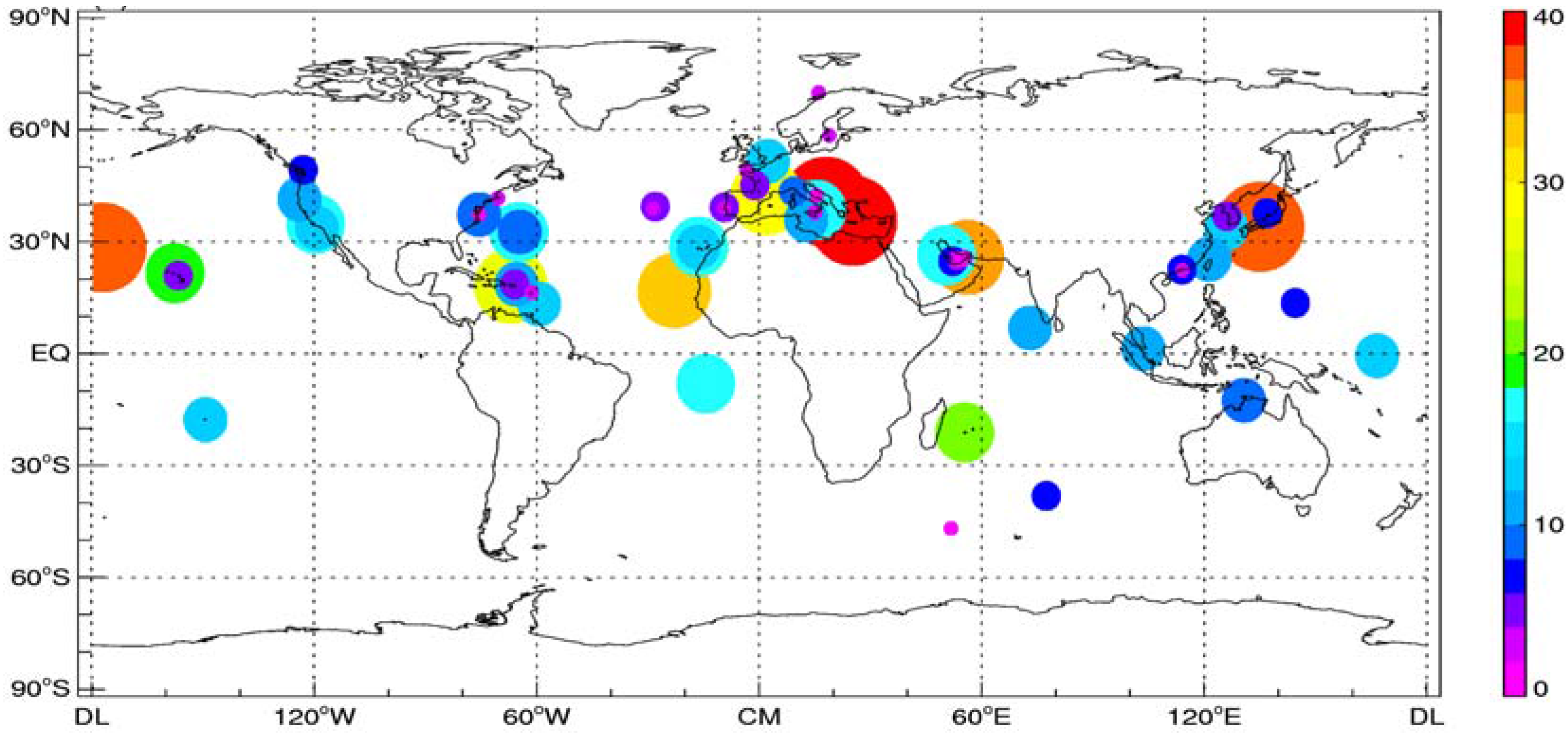
In order to put the performance of the GACP retrieval algorithm into current perspective, we applied the same regression analysis to the MODIS data. The MODIS instruments have a number of important advantages over the AVHRR, such as in-flight calibration, multiple spectral channels, higher radiometric accuracy, and higher data density. Figure 4 shows the geographical distribution of the MODIS-AERONET matches for the period 2003–2009. Comparing Figure 1 and Figure 4 we can conclude that the MODIS-AERONET matches are distributed more uniformly than the GACP-AERONET ones. Besides the higher data density of the MODIS dataset, this fact reflects the history of the AERONET network: while Figure 1 refers to the period 1995–2009, Figure 4 pertains to 2003–2009 when data from a larger number of AERONET stations became available. However even for MODIS the data matches are mostly concentrated in the 20°–45° NH belt, while open ocean areas are mostly underrepresented. The time series of the number of MODIS-AERONET matches shown in Figure 5 is similar in shape to the corresponding part of the GACP-AERONET matching dataset (cf. Figure 2) while being a factor of 1.5 to 2 greater.

Figure 4. As in Figure 1, but for MODIS-AERONET matches.

Figure 4. As in Figure 1, but for MODIS-AERONET matches.

The MODIS-AERONET scatter plot and regression lines are shown in Figure 6. We found the MODIS-AERONET correlation coefficient to be equal to 0.79, similar to the GACP value. The uniform, AERONET-only σ, and combined MODIS-AERONET σ weightings result in regression coefficients a of 1.08, 1.24 and 1.10, respectively, thereby exhibiting significant variation depending on the adopted weighting strategy. The spread of the MODIS regression coefficients is broader than in the case of GACP. The MODIS monthly mean values tend to be higher than the corresponding AERONET values, while for the GACP the opposite is true. Among possible explanations for this difference are the greater flexibility of the MODIS retrieval algorithm, wherein the microphysical aerosol model can be selected from several options, as well as the differentiation between darker open-ocean and brighter coastal waters not available for GACP retrievals.

We note that the regression results above should not be compared directly to the MODIS accuracy estimates in [28] mentioned in the introduction. This is because (i) we compare monthly mean values as opposed to instantaneous results in [28] (see the discussion of the differences between the two approaches in Section 2), and (ii) we use a single-parameter regression model as opposed to the slope-intercept model in [28]. Furthermore, the two analyses refer to different satellites (Aqua and Terra) and different time periods.

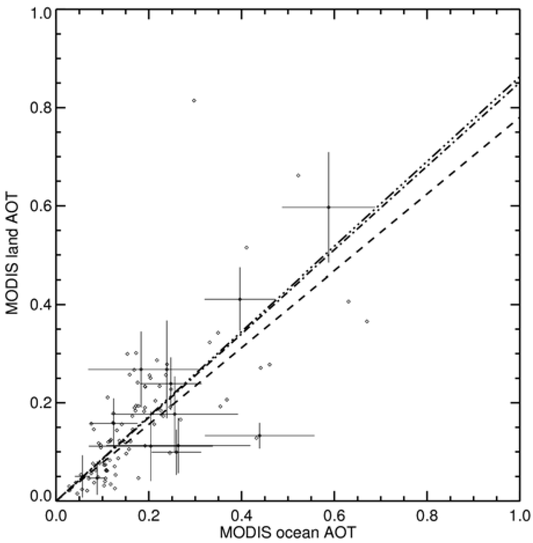
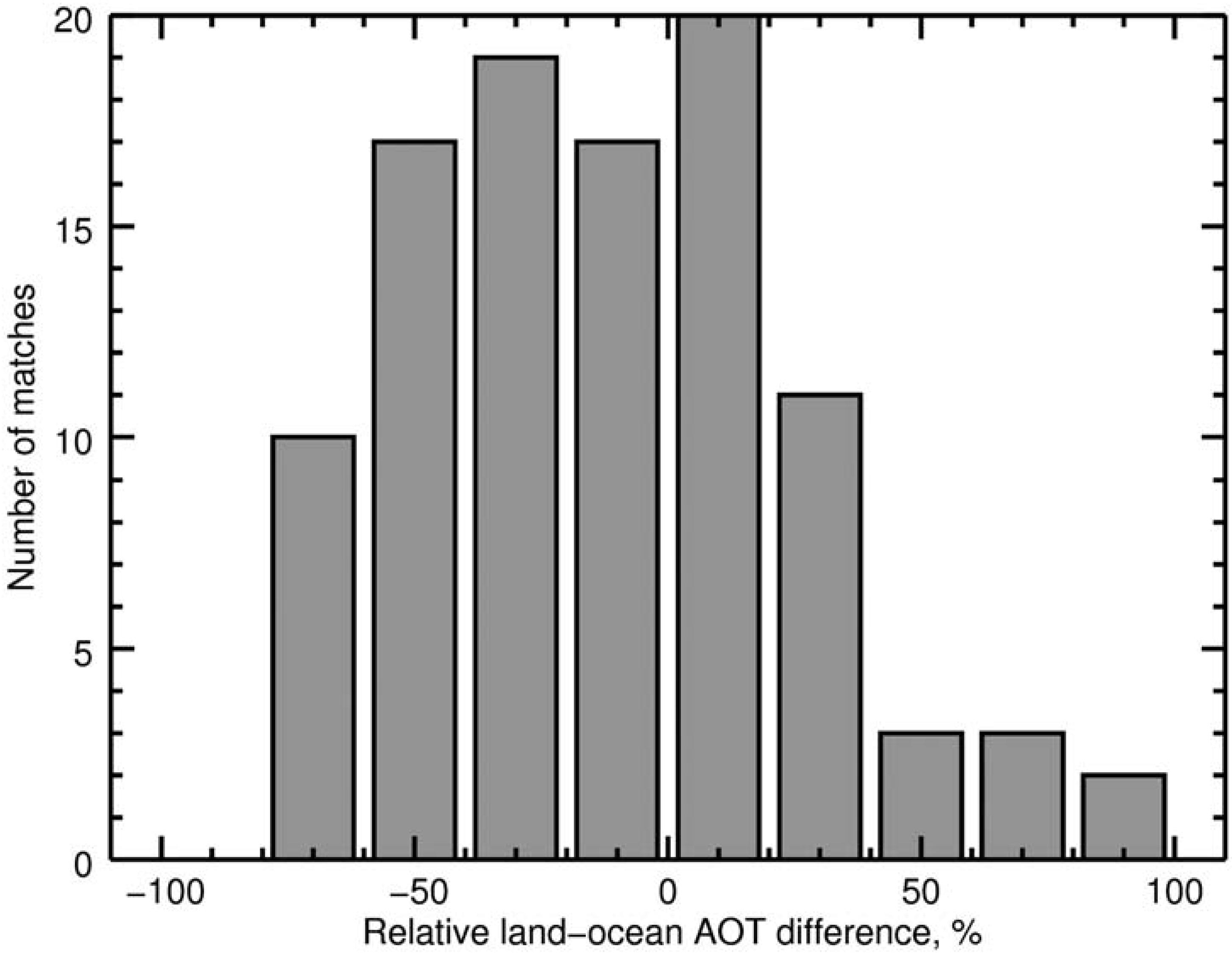
To investigate to what extent the local conditions at a coastal AERONET station may affect aerosol amounts, we calculated monthly mean AOT values using the MODIS data separately over the oceans and over land within a 200 km distance from the coastal stations where both types of retrievals were available. The results are presented in Figure 7 and Figure 8 as a scatter plot and a histogram of relative differences, respectively. One can see that over land, the monthly AOT averages tend to be smaller than the corresponding over-ocean values, with a regression coefficient between 0.78 and 0.86 and a correlation coefficient of 0.72. A negative bias is also clearly visible in the skewness of the histogram of the relative land-ocean differences (Figure 8) which can be as high as −70%. The observed differences may represent the range of actual land-ocean AOT gradients. They may also be affected by potential over-land and over-ocean aerosol retrieval algorithm biases related to the choice of aerosol and surface models and cloud screening. Further research is needed to establish the relative influence of these factors. Nevertheless these results suggest that coastal monthly mean aerosol amounts may differ significantly from open-ocean or inland values. This factor may limit the achievable accuracy of validation of open-ocean satellite retrievals using ground-based measurements at coastal locations.

Figure 5. As in Figure 2, but for MODIS-AERONET monthly matches.

Figure 5. As in Figure 2, but for MODIS-AERONET monthly matches.

Figure 6. Monthly MODIS AOT vs. monthly AERONET AOT. The horizontal and vertical bars show one standard deviation of the selected AERONET and MODIS values, respectively. Also shown are regression lines of the form y = ax for the uniform weighting (dot-dashed line, a = 1.08), for weighting with the AERONET σ (triple dot-dashed line, a = 1.24), and for weighting with the combined AERONET-MODIS σ (dashed line, a = 1.10). The correlation coefficient is 0.79.

Figure 6. Monthly MODIS AOT vs. monthly AERONET AOT. The horizontal and vertical bars show one standard deviation of the selected AERONET and MODIS values, respectively. Also shown are regression lines of the form y = ax for the uniform weighting (dot-dashed line, a = 1.08), for weighting with the AERONET σ (triple dot-dashed line, a = 1.24), and for weighting with the combined AERONET-MODIS σ (dashed line, a = 1.10). The correlation coefficient is 0.79.

Figure 7. Monthly over-land vs. over-ocean MODIS AOTs in the vicinity of coastal AERONET stations. Horizontal and vertical bars show one standard deviation of the selected values. Also shown are regression lines of the form y = ax for the uniform weighting (dot-dashed line, a = 0.85), for weighting with the AERONET σ (triple dot-dashed line, a = 0.86), and for weighting with the combined AERONET-MODIS σ (dashed line, a = 0.78). The correlation coefficient is 0.72.

Figure 7. Monthly over-land vs. over-ocean MODIS AOTs in the vicinity of coastal AERONET stations. Horizontal and vertical bars show one standard deviation of the selected values. Also shown are regression lines of the form y = ax for the uniform weighting (dot-dashed line, a = 0.85), for weighting with the AERONET σ (triple dot-dashed line, a = 0.86), and for weighting with the combined AERONET-MODIS σ (dashed line, a = 0.78). The correlation coefficient is 0.72.

Figure 8. Histogram of relative differences between monthly over-land and over-ocean MODIS AOTs for the data shown in Figure 7.

Figure 8. Histogram of relative differences between monthly over-land and over-ocean MODIS AOTs for the data shown in Figure 7.

5. MODIS-GACP Comparison

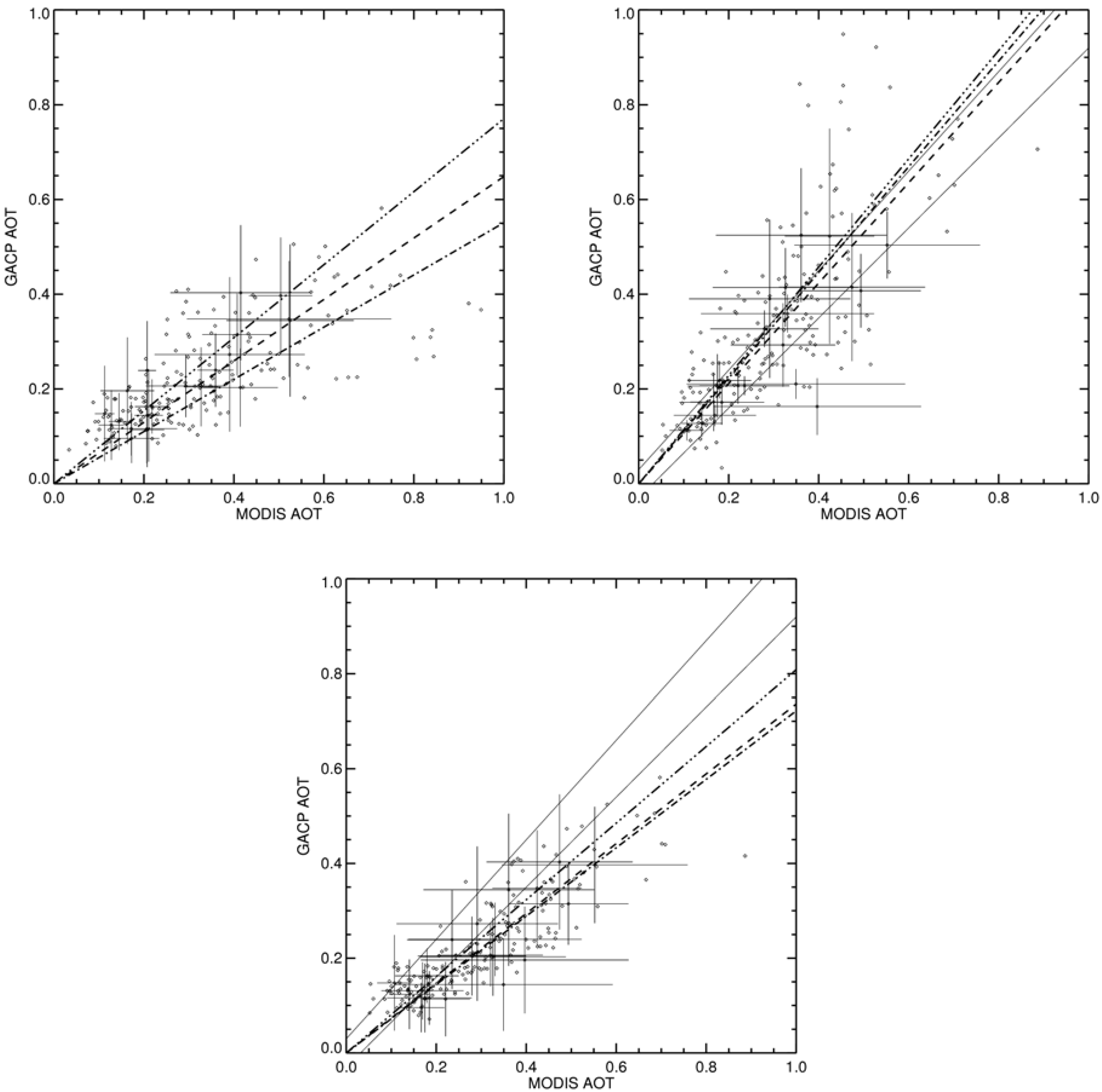
The identified differences between the GACP-AERONET and MODIS-AERONET relationships may partly be explained by the differences in the spatial and temporal distributions of the comparison points (cf. Figure 1 and Figure 4 and Figure 2 and Figure 5). It is therefore instructive to compare the two satellite datasets using the subset of matching AERONET monthly mean data points common to both. This comparison is presented in Figure 9, where the upper right and upper left panels show the GACP-AERONET and MODIS-AERONET regression lines, respectively, for locations for which the data from AERONET and both satellite datasets were simultaneously available. The bottom panel shows the GACP-MODIS comparison for the same sample. One can see that for the GACP, the regression coefficients remained essentially the same compared to the full set of matches (0.72 for the uniform weighting, 0.81 for the AERONET weighting, and 0.74 for the combined AERONET-GACP σ weighting) with a slightly higher correlation coefficient of 0.85. However, for the MODIS data the correlation coefficient decreased to 0.75. The MODIS regression coefficients decreased to 1.07 for the uniform weighting and to 1.05 for the combined AERONET-MODIS σ weighting. The reduction in the regression coefficient was especially significant for the AERONET-only weighting: from 1.24 to 1.12, demonstrating the important effect that the implicit weighting imposed by the choice of the comparison set may have. Thin solid lines in the upper panels of the figure show the MODIS uncertainty envelope (±0.03 ± 0.05τ_AERONET) for reference. Note, that the envelope refers to instantaneous comparisons, while the points in the plot represent a comparison of monthly mean values. As discussed in Section 2, the two approaches may not be directly compatible. The differences between the GACP-AERONET and MODIS-AERONET slopes identified in the upper panels of Figure 9 are most apparent on the GACP-MODIS scatter plot shown in the lower panel. The GACP-MODIS regression coefficients are 0.77 for the MODIS weighting, 0.65 for the GACP-MODIS weighting, and 0.55 for the uniform weighting. Notably the GACP-MODIS correlation coefficient of 0.62 is smaller than either the GACP-AERONET or the MODIS-AERONET one, thus suggesting that uncorrelated factors may be contributing to the discrepancies between either dataset and AERONET.

The question of why the MODIS-AERONET slopes are generally above one and the GACP-AERONET slopes below one for the coastal sites may require an additional extensive analysis of both satellite datasets.

As discussed in [35], due to the inherent limitations of the AVHRR instrument the most we may be able to do is to tune the a priori fixed parameters of the GACP retrieval algorithm to produce a globally “optimal” aerosol dataset. It would be preferable to base a systematic global test and the final tuning of the GACP retrieval algorithm on comparisons with more advanced satellite aerosol products, such as the MODIS one. Within such a framework, the presented GACP results would indicate that such a tuning is needed. However, our results indicate that a number of questions would need to be rectified before the actual tuning becomes warranted. These questions include the GACP-AERONET geographical mismatch, the peculiarities associated with the coastal AERONET sites, and the range of MODIS-AERONET discrepancies which is similar to the GACP results.

The MODIS aerosol retrieval algorithm is significantly more flexible than the GACP one. The reasons for the observed MODIS-AERONET discrepancies may, thus, be several and less straightforward to disentangle. One such reason may be that the MODIS algorithm often attempts aerosol retrievals in difficult conditions rejected by the simpler GACP algorithm. For example, some large MODIS-AERONET differences at AOT > 0.5 may be due to the problems with aerosol-cloud differentiation for such large AOTs. Such pixels would be screened out by the GACP algorithm and no AOT retrieval would be attempted. A greater number of MODIS retrievals in difficult conditions, which would necessarily be less accurate, may also explain why the MODIS correlation coefficient is similar or somewhat smaller than the GACP one.

One of the four anonymous reviewers of this paper suggested that comparing GACP and MODIS data over the open ocean in the absence of AERONET stations could be used to determine whether the identified discrepancies between the GACP and MODIS results are related to the inability of the GACP algorithm to model aerosols over coastal waters. However, such an analysis, by itself, is unlikely to help distinguish the upwelling radiance contribution of coastal waters to the observed discrepancies from other potential sources of uncertainty such as differences in the wind speed, aerosol type, and cloudiness. In addition, a recent study [30] has found that even AOT retrievals for near-perfectly collocated pixels (with matching observation times and locations and matching cloud screening decisions) coming from two advanced instruments (MODIS and MISR) on-board the same satellite exhibit large differences. Absolute AOT discrepancies of 0.07 are common over the ocean even for a 24-month averaging over 1° × 1° areas, and the origin of these discrepancies is still unknown. These results make it quite doubtful that a significant reduction in comparison uncertainty can be achieved without the use of external datasets to constrain variable observational conditions and of benchmark ground-based data such as AERONET.

Figure 9. AOT scatter plots of GACP vs. AERONET (upper left panel), MODIS vs. AERONET (upper right panel), and GACP vs. MODIS (bottom panel) for the common sample. Upper left panel: regression lines of the form y = ax for the uniform weighting (dot-dashed line, a = 0.73), for weighting with the AERONET σ (triple dot-dashed line, a = 0.81), and for weighting with the combined AERONET-GACP σ (dashed line, a = 0.74); the correlation coefficient is 0.85. Upper right panel: regression lines for the uniform weighting (dot-dashed line, a = 1.07), for weighting with the AERONET σ (triple dot-dashed line, a = 1.12), and for weighting with the combined AERONET-MODIS σ (dashed line, a = 1.05); the correlation coefficient is 0.75. Thin solid lines in the upper panels show the MODIS uncertainty envelope (±0.03 ± 0.05τ_AERONET) for reference. Lower panel: regression lines for the MODIS weighting (triple dot-dashed line, a = 0.77), for the GACP-MODIS weighting (dashed line, a = 0.65), and for the uniform weighting (dot-dashed line, a = 0.55); the correlation coefficient is 0.62.

Figure 9. AOT scatter plots of GACP vs. AERONET (upper left panel), MODIS vs. AERONET (upper right panel), and GACP vs. MODIS (bottom panel) for the common sample. Upper left panel: regression lines of the form y = ax for the uniform weighting (dot-dashed line, a = 0.73), for weighting with the AERONET σ (triple dot-dashed line, a = 0.81), and for weighting with the combined AERONET-GACP σ (dashed line, a = 0.74); the correlation coefficient is 0.85. Upper right panel: regression lines for the uniform weighting (dot-dashed line, a = 1.07), for weighting with the AERONET σ (triple dot-dashed line, a = 1.12), and for weighting with the combined AERONET-MODIS σ (dashed line, a = 1.05); the correlation coefficient is 0.75. Thin solid lines in the upper panels show the MODIS uncertainty envelope (±0.03 ± 0.05τ_AERONET) for reference. Lower panel: regression lines for the MODIS weighting (triple dot-dashed line, a = 0.77), for the GACP-MODIS weighting (dashed line, a = 0.65), and for the uniform weighting (dot-dashed line, a = 0.55); the correlation coefficient is 0.62.

6. Conclusions

We used monthly mean AOT data from a comprehensive set of coastal and island AERONET stations to evaluate the GACP retrievals. Good correlation exists between the GACP and AERONET monthly means, with the correlation coefficient exceeding 0.8. We found that the GACP monthly means are on average 20%–25% lower than the corresponding AERONET values, depending on the regression weighting assumptions for the comparison dataset. A large discrepancy exists in the geographical coverage of the AERONET and GACP data, with the majority of the open-ocean areas being largely underrepresented. Possible peculiarities of coastal aerosols and differences between coastal and open-ocean water color makes questionable the generalization of these results on the entire GACP dataset. In addition, we show that monthly AOT variability makes the regression analysis results dependent on the particular choice of the comparison dataset and weighting assumptions.

To further evaluate the performance of the GACP algorithm in comparison with the AERONET measurements, we used the AOT data from MODIS. The regression analysis of MODIS and AERONET data revealed similar limitations. We found the MODIS monthly AOT means to be, on average, 5%–25% higher than the corresponding AERONET values, depending on the weighting assumptions for the comparison dataset. The correlation coefficient was slightly smaller for the MODIS-AERONET comparison, at 0.74–0.79.

Overall, the comparison with the AERONET monthly means has revealed similar performance of the two satellite datasets with a tendency of the GACP AOTs to underestimate and the MODIS over-ocean AOTs to overestimate the AERONET values. The range of these discrepancies is comparable to the uncertainties associated with the limited number of coastal and island stations and natural aerosol variability.

The comparison of monthly over-land and over-ocean MODIS AOTs in the vicinity of coastal AERONET sites showed that over-land values are, on average, 15%–20% lower than the corresponding over-ocean ones. While the biases in land and ocean retrieval algorithms and cloud screening procedures may not be excluded, these results indicate that aerosol loading in coastal locations may differ significantly from that in adjacent open-ocean areas, thereby limiting the achievable validation accuracy.

We conclude that significant limitations exist for the validation of over-ocean GACP aerosol retrievals using coastal AERONET stations. These limitations can be linked to the extreme sparsity of the open-ocean AERONET data, uncertainties associated with local conditions at the coastal stations, and regression accuracy limits imposed by natural aerosol variability. The development of the Maritime Aerosol Network (MAN) [36] which collects ship-based AOT measurements and is operational since late 2006 may eventually help mitigate these problems. Although the number of measurements from hand-held devices on moving ships is necessarily limited compared to the automated AERONET stations, especially if one attempts to estimate monthly means, much of the MAN data come from open-ocean areas, where no other ground-truth data are available. As more open-ocean sunphotometer data are accumulated and the GACP record is extended beyond 2009, the number of matching points between the two datasets may become sufficient to attempt the reduction of the current uncertainties. This task will be greatly facilitated by the planned switch of the GACP processing from the 30 × 30 km ISCCP DX product to a new 10 × 10 km ISCCP product. The switch to this product, presently being developed [16], will result in a nine-fold increase of the sampling density.

Our confidence in GACP results does not rely solely on the presented comparison with the AERONET results, but also on many validation efforts undertaken over the course of the dataset existence. These include comparisons with ground-based data, consistency checks, and inter-comparisons with satellite datasets and are outlined in the introduction. Given the identified uncertainties, the results of this study do not contradict these previous validation efforts. Future research may reduce these uncertainties and require modifications to the GACP algorithm.

We note that a larger number of more uniformly distributed AERONET measurements would allow for a better constrained comparison with satellite aerosol products over oceans. Currently the AERONET data represent a de facto standard source of ground-truth data for satellite product validation. The identified geographical mismatch of land-based AERONET stations and over-the-ocean satellite aerosol products is unlikely to completely disappear in the near future due to the difficulty of collecting open-ocean aerosol measurements. We, therefore, see the value of our study in quantifying the potentially achievable accuracy for validation of global satellite aerosol products.