Article

MODIS-Based Fractional Crop Mapping in the U.S. Midwest with Spatially Constrained Phenological Mixture Analysis

1
Department of Geography, University of South Carolina, 709 Bull St., Columbia, SC 29208, USA
2
Department of Geography, University of Wisconsin-Milwaukee, Milwaukee, WI 53201, USA
*
Author to whom correspondence should be addressed.
Remote Sens. 2015, 7(1), 512-529; https://doi.org/10.3390/rs70100512
Submission received: 17 September 2014 / Accepted: 23 December 2014 / Published: 6 January 2015
(This article belongs to the Special Issue Recent Advances in Remote Sensing for Crop Growth Monitoring)

Abstract

:
Since the 2000s, bioenergy land use has been rapidly expanded in U.S. agricultural lands. Monitoring this change with limited acquisition of remote sensing imagery is difficult because of the similar spectral properties of crops. While phenology-assisted crop mapping is promising, relying on frequently observed images, the accuracies are often low, with mixed pixels in coarse-resolution imagery. In this paper, we used the eight-day, 500 m MODIS products (MOD09A1) to test the feasibility of crop unmixing in the U.S. Midwest, an important bioenergy land use region. With all MODIS images acquired in 2007, the 46-point Normalized Difference Vegetation Index (NDVI) time series was extracted in the study region. Assuming the phenological pattern at a pixel is a linear mixture of all crops in this pixel, a spatially constrained phenological mixture analysis (SPMA) was performed to extract crop percent covers with endmembers selected in a dynamic local neighborhood. The SPMA results matched well with the USDA crop data layers (CDL) at pixel level and the Crop Census records at county level. This study revealed more spatial details of energy crops that could better assist bioenergy decision-making in the Midwest.

Graphical Abstract

1. Introduction

The Midwest is one of the major agricultural regions in the United States. In 2007, the Midwestern states had a market value of over $76 billion for crops (corn, soybean, wheat, and forage grass) and livestock [1]. Currently corn grain is still the most commonly utilized feedstock for ethanol [2]. With increased biofuel demand, food security and environmental contamination from intensified corn cropping become major concerns in this region [3]. Perennial native prairie grasses are recognized as promising alternative energy crops for cellulosic feedstock [4]. The USDA National Agricultural Statistics Service (NASS) publishes annual cropland data layer (CDL) products, in which annual crops are classified from satellite images at 30–56 m resolutions [5]. Perennial crops, however, are not examined in these products. To assist with sustainable bioenergy land use, there is a need for accurate mapping of energy crops in this important agricultural region.
Remote sensing has been proven to be an effective tool of regional and global agricultural monitoring. Aside from the U.S. CDL products from medium-resolution imagery, global cropland extents and irrigated areas have been extracted from frequently observed, coarse-resolution data [6,7]. A comprehensive review was presented in [8] about studies of global croplands and their water use with remote sensing and non-remote sensing approaches by the world’s leading researchers. Yet, even with high spatial-resolution imagery, mapping of individual crop types is often limited to large fields with homogeneous structures [9]. In complex agricultural areas with a diversity of crops, different crops often have similar spectra during the growing season. It is thus difficult to delineate crops using regular binary classifiers [10]. For satellite images at coarse resolutions, the mixed-pixel problem also results in uncertainties in crop delineation.
In the temporal domain, seasonal variations of the normalized difference vegetation index (NDVI) are closely related to phenological features such as the onset dates of green-up, peak growth, and senescence along vegetation development [11]. Phenology of annual crops is associated with their planting dates and development cycles in growing seasons. For example, corn is usually planted 1–2 weeks earlier than soybeans, but both have similar growth cycles along the season. Winter wheat is planted in winter and primarily grows in early spring. Spring wheat has a narrow growth cycle due to cold weather in the north. For perennial crops, cool-season grass (CSG) starts its growth in early spring and reaches peak growth in May, while warm-season grass (WSG) starts in later spring and has delayed Peak dates [12]. In addition, CSG turns to dormancy in hot, dry summers and has a second growth peak in the fall, while WSG remains green in summer. These phenological differences provide important information for crop mapping with repeated satellite observations [13,14,15]. Relying on these unique phenological features, multi-temporal, medium-resolution satellite imagery has been used for national mapping products such as the annual CDL maps [4] and the National Land Cover Databases (NLCD) [16] in the conterminous United States. Due to the tremendous amount of such satellite scenes needed in these products, the classification processes are time-consuming and labor-/cost-intensive. Moreover, limited by their coarse revisit cycles (e.g., 16-day interval for Landsat) and frequent contamination from cloud cover in the growing season, it is often difficult to extract stable phenological features from these data series for regional mapping processes.
The Moderate Resolution Imaging Spectroradiometer (MODIS) satellite product has been available since 2000. Its capabilities for daily observation and global coverage allow for efficient monitoring of seasonal crop development in large regions [17] and operational cropland estimation [18]. Algorithms using MODIS time series to derive phenological parameters have also been developed for crop mapping and monitoring its interannual dynamics [12,15]. At 250–1000 m resolution, a MODIS pixel often covers multiple crop fields on the ground. It reduces the accuracies of crop mapping, and smaller crop clusters are often lost with conventional binary classification approaches [15]. This may severely affect regional crop analysis that relies on the accuracies of crop delineation [19].
Spectral mixture analysis (SMA) has been widely used to extract sub-pixel information of land covers based on their spectral differences [20,21,22]. Recently, some efforts were made to extract sub-pixel land covers with crop phenology from MODIS time series [23,24], the so-called phenological mixture analysis (PMA). Both methods share the same principle, i.e., the SMA approaches improve the spatial resolutions with spectral signature of crops, while the PMA approaches perform the same process with their temporal signatures. However, two major challenges remain: (1) appropriate selection of endmembers [20,25]; and (2) identifying the correct signatures that characterize crops. Differences in spectral or temporal signatures of the same class (endmember variability) may significantly affect the accuracies of sub-pixel land cover fractions [21,25]. To reduce these in-class differences, Deng and Wu [22] developed a spatially adaptive spectral mixture analysis, in which spatial patterns were used to overcome the endmember variability in extracting sub-pixel impervious surfaces in urban lands. The idea of spatial adjustment could also be employed in crop unmixing and regional crop mapping.
This study aims to combine the phenology-based mapping and unmixing approaches to extract in-pixel fractional crop covers in the Midwest using MODIS time series in 2007. A spatially constrained PMA (SPMA) approach was developed to overcome the challenges in regular unmixing processes. The results were validated with the 56-m CDL products in the region. The extracted crop planting acreages were also compared with the county-level Crop Census records in the same year. Findings in this study provide spatially detailed information about bioenergy land use in the Midwest.

2. Materials and Methods

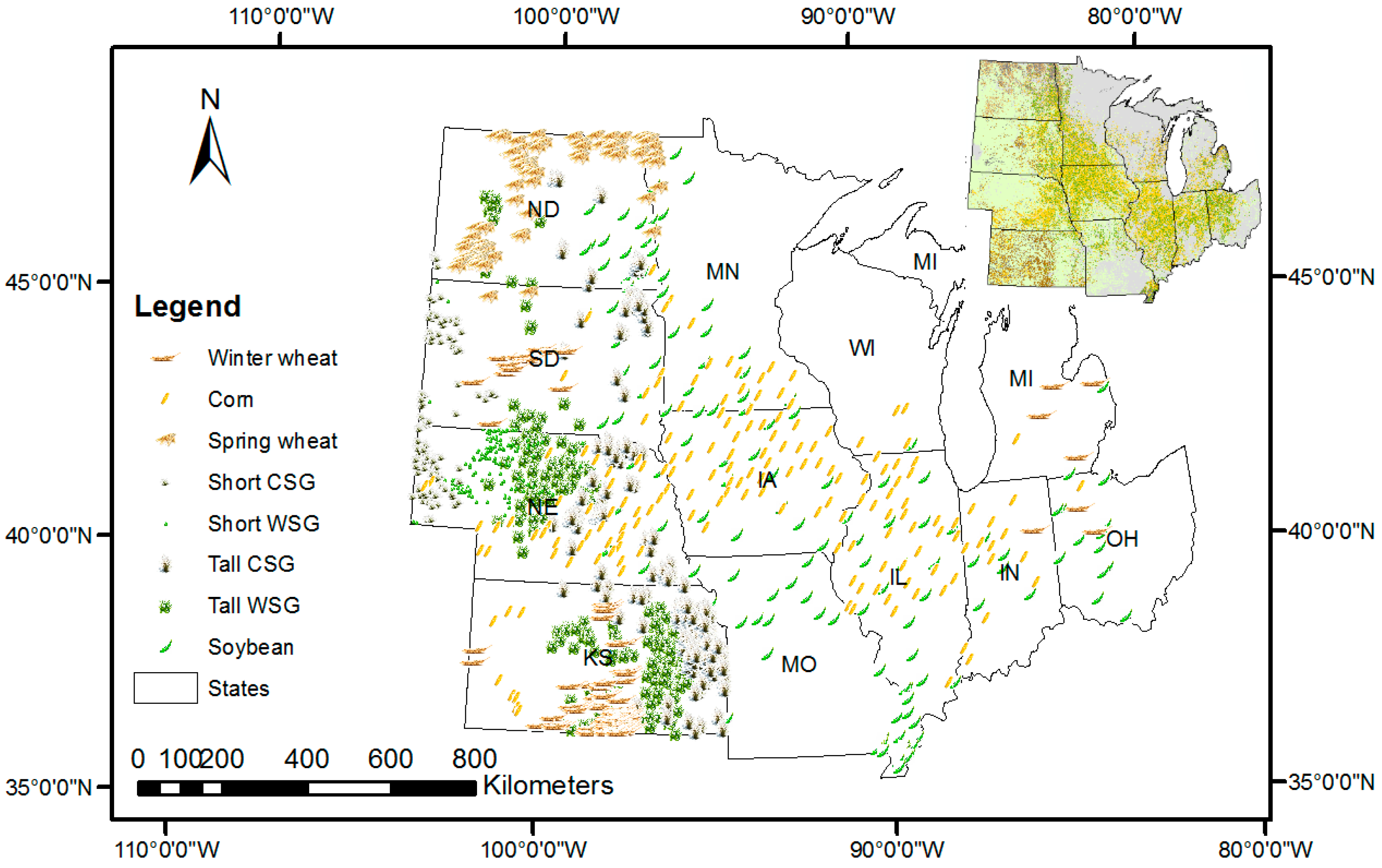
2.1. Study Area and Data Sets

The U.S. Midwest is composed of 12 states across the central United States (Figure 1). Topography gradually changes from the arid highlands in the west to gently rolling hills and semi-humid flat lands along the west-east gradient. Prairies cover most of the Great Plains in the western states, while cultivated lands dominate other states across the region—the so-called Corn Belt. Agriculture is the largest driver of local economies in the Midwest, accounting for billions of dollars’ worth of exports of grain and livestock production [1]. Corn/soybean shift planting is the common cropping pattern. The extended area grows winter wheat in southern states and spring wheat in the north. The warm-season prairie grasses grow natively across the tallgrass prairie, covering two-thirds of the Midwest [2]. Although more than 90% of tallgrass prairie lands have been cultivated since the European settlement in the 1830s, WSG remains in prairie remnants and is often mixed with introduced, highly productive CSG species in pasturelands.
Accompanying the increased corn ethanol production, expansion of corn planting areas has been recorded in national Crop Census records surveyed by USDA NASS. In 2007, corn acreage reached its historical record (after 1944) of 93.6 million acres, as high as 19% up from 2006 [1]. Ten of the 12 Midwestern states (except Missouri and Minnesota) are marked among the nation’s top 10 states for ethanol production capacity [26]. Although cellulosic technology is still in its early stage, crop residuals and prairie native grasses are treated as a promising alternative biofuel feedstock in the Midwest [2,5].
Figure 1. The study area of the Midwest and an example MODIS NDVI composite in 2007 (Day-of-Year 137/177/105 as B/G/R).
Remotesensing 07 00512 g001
The 8-day, 500-m MODIS surface reflectance products (MOD09A1) in 2007 are the primary satellite data in this study. The Midwest can be almost fully covered by four MODIS tiles. For each MODIS tile, all MOD09A1 scenes in 2007 were downloaded from the Land Processes Distributed Active Archive Center and re-projected to the North America Datum 1983. NDVI was then extracted from the red and near infrared spectral bands of each MODIS scene, mosaicked and clipped to the Midwest region, and stacked to 46-scene NDVI time series. The time series was finally smoothed with a five-point median filter followed by the Savitzky-Golay filtering method [2,27]. The example NDVI composite in Figure 1 demonstrates the clustering patters of crops in the Midwest. The 250-m MODIS NDVI products such as MOD13Q1 [14] were not used in this study because of their longer temporal intervals (16-day). As revealed in previous studies [2], at such temporal resolution the subtle biophysical differences in critical growing stages are often lost.
The CDL products were downloaded from USDA NASS [28]. In 2007 the CDL maps were classified from the Indian RESOURCESAT-1 Advanced Wide Field Sensor (AWiFS) imagery acquired in the growing season, with generally 85%–95% accuracies for major crop-specific land cover categories [4]. At 56-m resolution, they could serve as the reference for crop classification in this study. To simplify the process, only corn, soybean, winter wheat, spring wheat fields, and perennial lands were considered in this study. Other crops and non-crop covers were blacked out from the CDL map. Additionally, the NASS county-level Crop Census records were downloaded and used as a secondary data source for crop planting acreages.
Training data of annual crops (corn, soybean, winter wheat, and spring wheat) were selected from the 2007 CDL map. A layer covering the four annual crops was extracted from the raw CDL map and aggregated to 500 m cell size with the following process. In a given 500-m cell, the percentage of each crop was calculated as the ratio of the number of CDL pixels of this crop to the total CDL pixels in the 500 × 500 m2 square. Therefore, the re-processed 500 m CDL data actually contained the percent cover layers of the four annual crops. In the percent cover layer of each crop, subsets of 5 × 5 pure cells (100%) were extracted and their central locations were collected as ground truth sample points. To reduce errors induced from CDL classification, NDVI time series of these samples were individually examined based on a crop’s specific phenological patterns in accordance with crop calendars. A total of 172 sample points for corn, 96 for soybean, 103 for spring wheat, and 100 for winter wheat were randomly collected as their training samples (Figure 2).
Figure 2. Training data sets of the eight crops in the study area. CSG and WSG represent cool-season and warm-season grasses, while Tall and Short indicate tallgrass and shortgrass floristic regions. The inset is the 2007 CDL map of the region.
Remotesensing 07 00512 g002
For perennial crops, the WSG and CSG distributions were not available in any public agricultural databases. In this study, their ground truth samples were extracted from a previously published grass abundance map of plant function types (PFT) in the Great Plains [15], in which a phenology-assisted decision tree was developed to identify different PFT (C3 and C4) grasses in two floristic regions (shortgrass and tallgrass) with yearly MODIS NDVI time series in 2000–2009. The overall classification accuracies reached about 22%. At a given pixel with 10 years’ classification results, abundance of a grass type was approximated by the frequency of its occurrence of a grass type in 10 years (in percent). The C3 grass was actually the CSG while C4 was WSG of our study here. Considering geographic differences in both PFT and floristic regions of the Great Plains, we randomly extracted pure (>80%) samples of four grass types: shortgrass CSG (132), shortgrass WSG (143), tallgrass CSG (182), and tallgrass WSG (188). Only four Midwestern states (ND, SD, NE, and KS) are covered in the Great Plains and, therefore, sample points of these grass types were clustered in the west of the study region (Figure 2).

2.2. Methodology

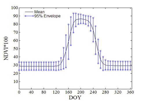
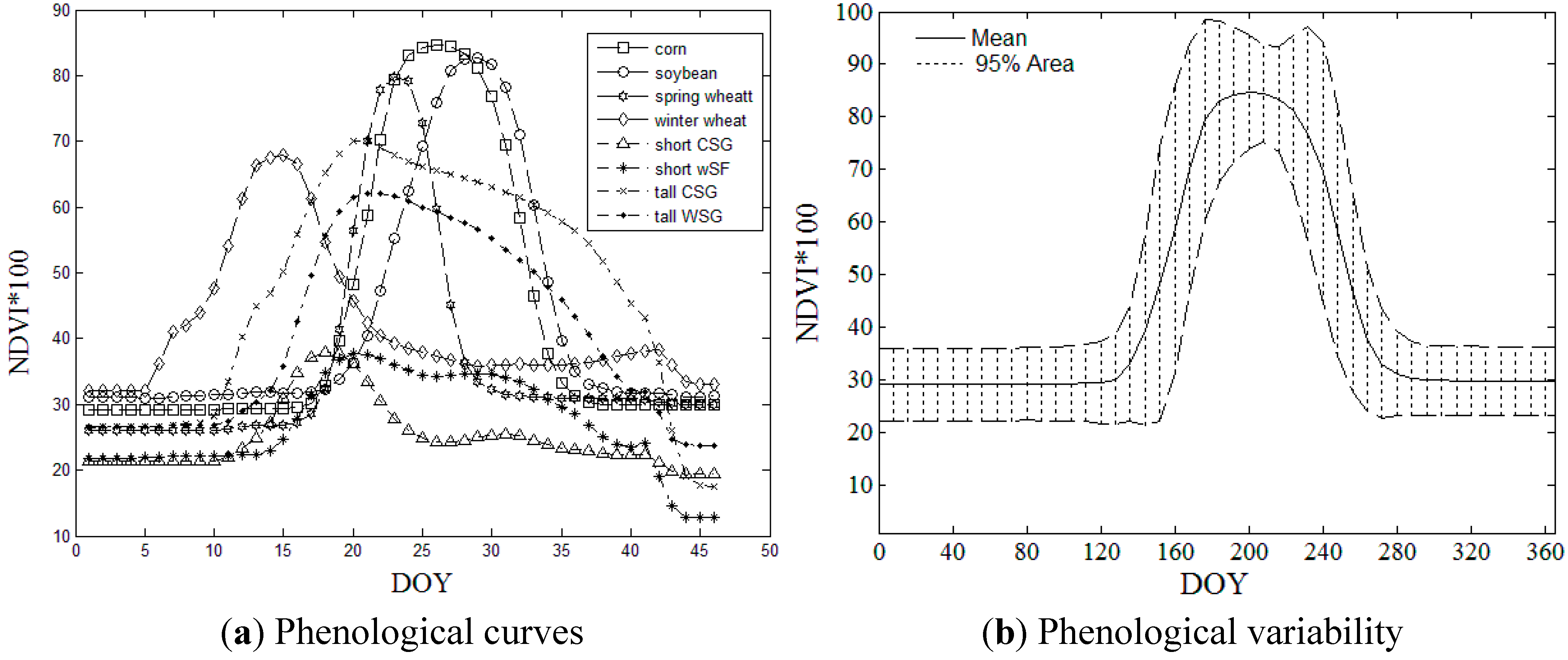
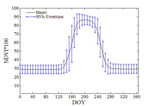
2.2.1. NDVI Time Series and Crop Phenology

For each crop, the NDVI values of all training samples were averaged at each time interval. The averaged NDVI time series in Figure 3a reflects the crop’s general growth cycle and phenological characteristics. Corn was planted slightly earlier than soybeans and had similar growth cycles throughout the season. Winter wheat had the earliest growth in spring. Spring wheat had the narrowest growth cycle. Perennial grasses had much longer growing season than annual crops. Tall grasses always had higher NDVI values than short grasses. These unique phenological features were useful in delineating these crop types.
Figure 3. The smoothed NDVI time series of the eight crops (a) and phenological variability using corn as an example (b). The X-axis represents the Day-of-Year (DOY) of data acquisition dates in 2007.
Remotesensing 07 00512 g003
The phenological curves in Figure 3a may vary at different geographical locations. It is commonly recognized that crop phenology relies on local environmental conditions. As an apparent phenomenon, for example, a crop’s planting or greenness onset dates in the north could be a few weeks later than those in the south. The Midwest covers 15° in latitude across the region. The shift of crop phenology in such a huge region could be dramatic, which leads to considerable phenological variability in the crop. Figure 3b demonstrates the phenological variability of corn by displaying the 95% envelopes of its NDVI variation at each interval. Variations in critical growing stages such as start of growth and senescence (the NDVI variation along the slopes) are much larger than other stages. The average variation for each crop could be simply calculated as the mean of the 46 standard deviations of NDVI along the year. In Table 1, the average variation reaches 5–10 (in the unit of NDVI × 100) for the eight crops. Tallgrass crops had higher average variation because of their heterogeneous growth conditions. The average variation of winter wheat was even higher than 10 due to the dramatic difference of winter conditions in such a large region. The “stddev” in the table is the standard deviation of the 46 standard deviations of NDVI along the year. Its large values indicated large dynamics of the variability in different growing periods along the year. Therefore, it is not suitable to assign the globally averaged phenological curves in Figure 3a as crop endmembers in the unmixing process. Here we established a spatially constrained rule to reduce these uncertainties.
Table 1. Descriptive statistics of the 46 standard deviations of the eight crops.
CropsCornSoybeanSpring WheatWinter WheatShort CSGShort WSGTall CSGTall WSG
mean5.476.566.1710.44.703.797.316.61
stddev *3.132.642.142.941.281.793.402.49
* stddev denotes the standard deviation.

2.2.2. Spatially Constrained Phenological Mixture Analysis (SPMA)

The phenological curves in Figure 3a are not always distinctive in all MODIS pixels. At coarse resolution, a pixel often covers multiple crops on the ground. Its NDVI time series is thus a combination of multiple phenological curves. Following the logic of linear spectral mixture analysis, we assumed that the NDVI of a mixed pixel was a linearly weighted contribution from multiple crops in the pixel. It can be written as:
R i = i = 1 N r i j x j + ε i with   j = 1 N x j = 1   and   0 x j 1
Where Ri is the NDVI value at time i of the mixed pixel (1≤ i ≤ 46), rij is the NDVI of endmember j at time i. xj is the fractional cover of endmember j, and N is the number of endmembers (N ≤ 8 in this study). εj is the error term at each time.
Endmember selection is a challenge to all unmixing methods. In a mixed pixel, non-representative endmembers result in dramatic classification errors. In this study, phenological variation of crops (as shown in Figure 3b) at different geographic locations cannot be ignored in such a large region. Here we developed a spatially constrained rule to optimize the endmember selection process. The basic hypothesis of the approach is that crop growth and distribution are spatially constrained to environmentally similar conditions. For the same crop type, plants growing nearby share similar water, soil, weather conditions, and management activities, and therefore have more similar phenological curves than those planted farther apart. Past studies have shown that crops have their own clustering patterns across the Midwest. For example, winter wheat is most common in southern states such as Kansas while spring wheat only grows in northern states such as North Dakota and South Dakota, and short grasses are only available in the arid and cold uplands in western states. Therefore, it is reasonable to assume that the phenological curves of a crop growing in a local cluster do not vary much.
Under this hypothesis, pure pixels of a crop from a spatial neighborhood are selected and their averaged phenological curve serves as its endmember in Equation (1). Scanning method is commonly employed to find objects in neighborhoods [21]. When dealing with huge area and relatively less pure pixels in this study, however, it becomes time-consuming and unreliable. Here the spatial distance between any given pixel and the training data set is employed to find the nearest pure pixels. To be computationally efficient in this large region, we used the absolute distance to substitute the Euclidean distance:
D x y = | x i y i | + | x j y j |
To initiate the process, at a given pixel the nearest 10 pure pixels (from training data) were set as an empirical threshold of spatial constraints. If a crop had multiple pure pixels in this constraint, its phenological curve was averaged and used in Equation (1). The threshold 10 was determined here based on our repeated tests to balance the accuracy and computation efficiency. When the threshold was too small, the phenological curves of crops were less representative and resulted in large confusion in mixed pixels. When the threshold was set larger (>10), the process became time-consuming and small clusters of a crop were omitted due to its limited pure pixels in the neighborhood. Also, the CDL map in Figure 2 (inset) demonstrates the clustering patterns of annual crops. To better identify these small crop clusters, it was reasonable to assume that at least three crops grow in a local area (e.g., corn, soybean, and CSG grass in the Corn Belt). However, in Figure 2 pure pixels of crops at 500 × 500 m2 cell size are not randomly distributed all over the Midwest. In cases where pure pixels of fewer than three crops can be found in this constraint, the search moves to the nearest 20 pure pixels, and so on. It should be noted that the method heavily relied on the distribution of pure pixels. Pure pixels of grasses were clustered in the west of the region (Figure 2) because their training data were only available in four Midwestern states (ND, SD, NE, and KS). Of the CDL products, tallgrass still commonly grows in pasturelands of other states. Therefore, we always used the nearest five pure pixels of tallgrass (WSG or CSG) in the search, although the distance could be larger than 20 pixels.

2.2.3. Accuracy Assessment

Validation samples of annual crops were re-processed from the 2007 CDL product in the study region. For a given crop, a number of sample points were randomly selected on the aggregated CDL percent cover layers (500 m cell size). At any point, percent cover of a crop was the average of a 3 × 3 local window centered at this point. One hundred fifty random samples were selected for corn and soybeans and 50 samples for spring wheat and winter wheat, respectively. As shown in Figure 2 (inset), the growth of wheat is clustered in the Midwest, with spring wheat in the northern states (ND and SD) and winter wheat in the southern states (especially KS). Their distributions are much lower than for corn and soybeans. Therefore, we selected a smaller size of validation samples for each crop. Validation samples of perennial grasses were randomly extracted from the ranked (at a 10% interval) grass abundance map published by [15]. One hundred fifty random samples were selected for tall grasses, and 50 samples for short grasses, similarly. To be comparable, we grouped the SPMA-extracted results of each perennial crop into the corresponding ranks. Finally, the SPMA-extracted results were also averaged in a 3 × 3 local window centered at each sample point.
With these validation samples, two common indicators were used to assess the accuracies of the SPMA-extracted crop percent covers by assuming the CDL outputs as references. The root mean square error (RMSE) quantifies the relative errors of the SPMA abundance at the pixel level, while the systematic error (SE) indicates an overall tendency of upward or downward estimation bias [29]. These accuracy metrics can be calculated as:
R M S E = i = 1 N ( r i x i ) 2 N
S E = i = 1 N ( r i x i ) N
where xi is the SPMA-extracted crop percent cover at sample i, ri is the corresponding percent cover from the CDL-summarized reference, and N is the total number of samples.
Crop planting acreages can be summarized at the county level from the SPMA-extracted percent covers. To assess their accuracies by assuming the Crop Census records as references, we used a mean relative area error (MRAE) to reduce the size effects of different counties:
M R A E = i = 1 N ( r i x i ) r i / N
where xi is the SPMA-extracted crop area (in acres) in county i, ri is the surveyed crop area from the NASS Crop Census records, and N is the total number of counties in the Midwest.

3. Results and Discussion

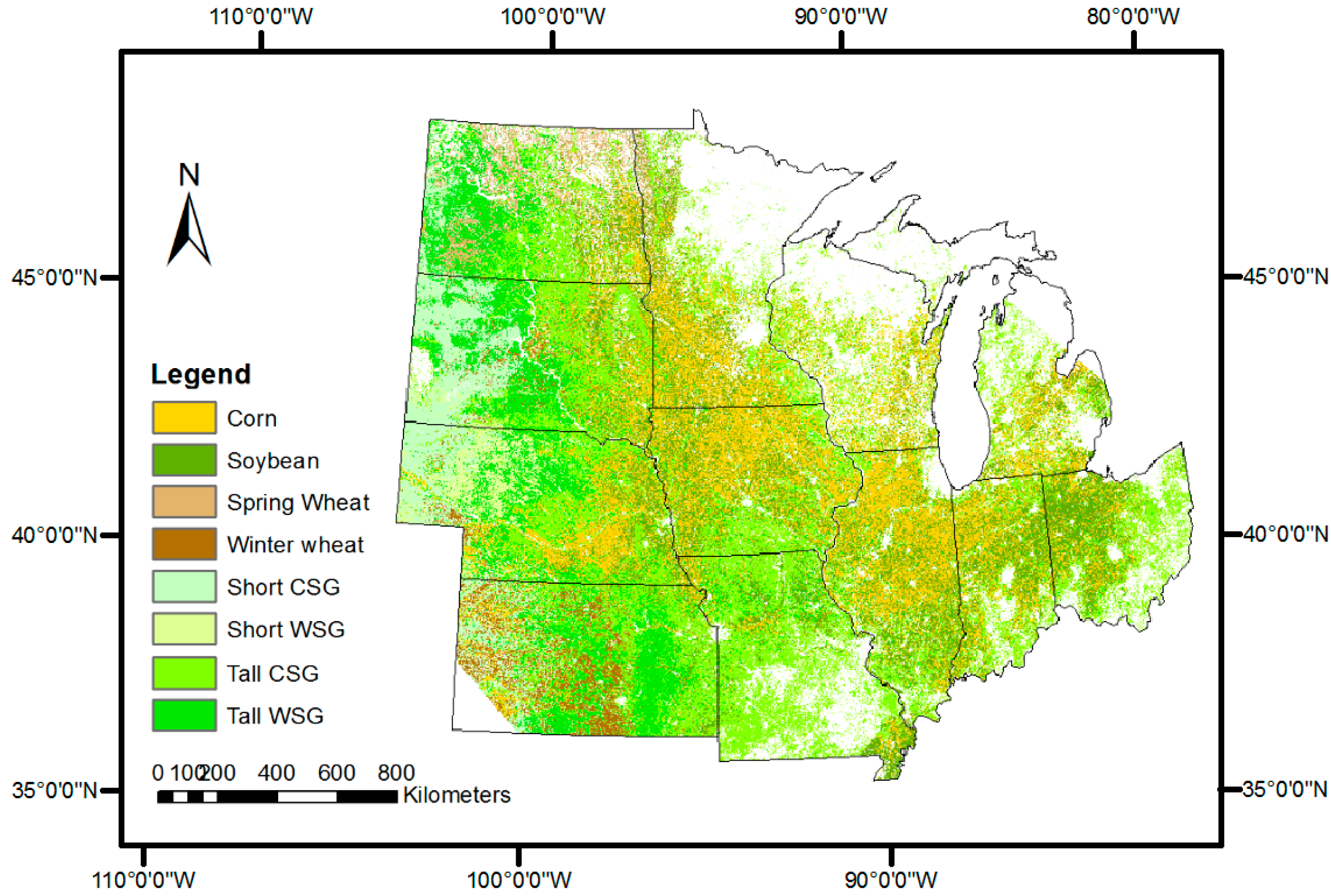
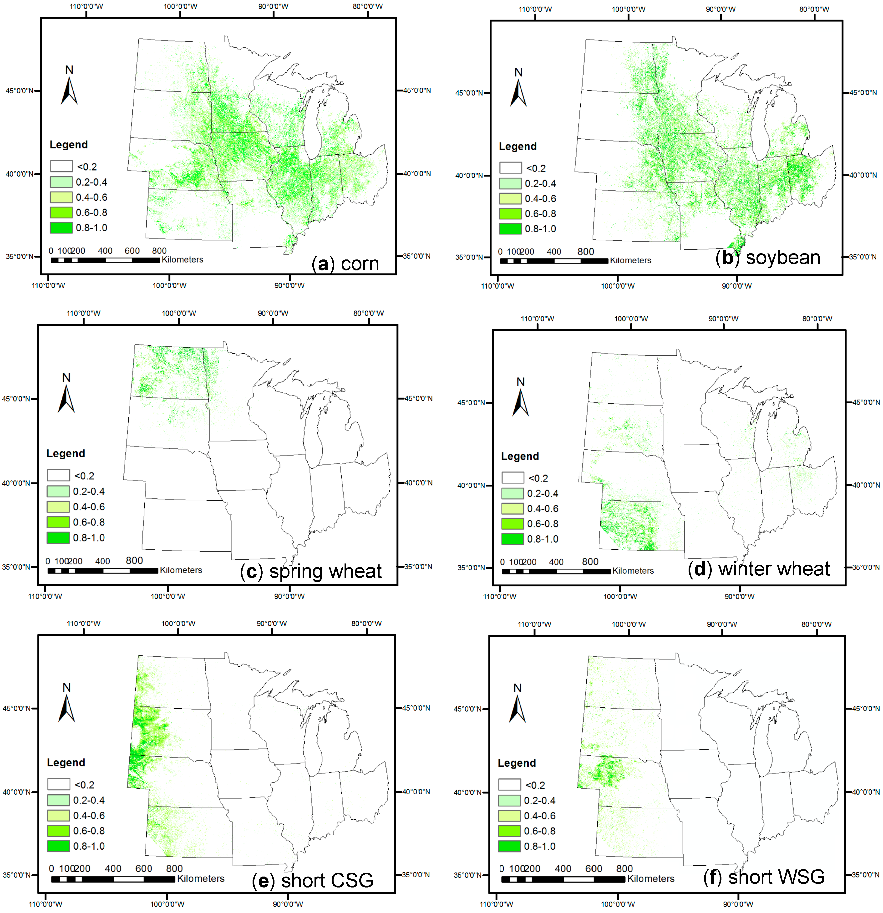
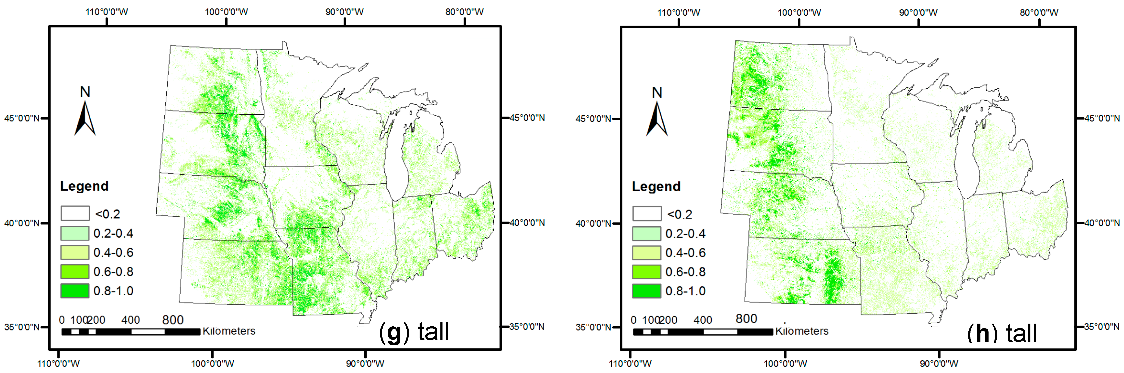
3.1. SPMA-Extracted Crop Percent Covers

The SPMA approach calculated the percent covers of all crops. Assigning the pixel to a crop that has the largest cover, crop distributions in the Midwest were extracted from MODIS time series (Figure 4). The general patterns agreed with the CDL product, showing the apparent corn and soybean domination in the Corn Belt, spring wheat in the north, and winter wheat in the south. Grasses dominated the western states. The native prairie remnants identified in [15], such as the Flint Hills (tallgrass prairie) in KS and Sand Hills (tallgrass/shortgrass mixed-grass prairie) in NE, were also extracted in the figure.
Figure 4. The SPMA-extracted dominant crop distributions in the Midwest.
Remotesensing 07 00512 g004
In the percent cover maps, corn (Figure 5a) was the primary crop of the region and was mainly distributed in Iowa, Illinois, Indiana, southern Minnesota, and eastern Nebraska. The predominant distribution of corn in 2007 was consistent with the Crop Census records that corn planting areas reached a historical record in this year. Soybeans (Figure 5b) grew in the same area but had less coverage than corn. Most corn and soybean pixels were a mixture of each other because of their shift planting patterns, commonly observed in the Midwest. Spring wheat (Figure 5c) was clustered in North Dakota, South Dakota, and Minnesota, adapting to the cold weather in this area. Winter wheat (Figure 5d) was primarily clustered in Kansas, with expanded planting areas in Nebraska and South Dakota. Their spatially different clustering patterns revealed the climatic impacts on crop planting, and supported the spatial constraint strategy in this study.
Figure 5. The SPMA-extracted percent cover distributions of the eight crops: corn (a), soybean (b), spring wheat (c), winter wheat (d), cool-season shortgrass (e), warm-season shortgrass (f), cool-season tallgrass (g), and warm-season tallgrass (h).
Remotesensing 07 00512 g005aRemotesensing 07 00512 g005b
Shortgrass in the west of the region extended from the shortgrass prairie in the Great Plains. Cool-season shortgrass (Figure 5e) dominated in the Black Hills along the west edge of South Dakota, adapting to the cold, upland climates. Warm-season shortgrass (Figure 5f) mainly grew in the Sand Hills, Nebraska, a typical mixed-grass prairie and the largest unplowed prairie remnant in the United States. Cool-season tallgrass (Figure 5g) distributes all over the Midwest because it has been commonly planted as a productive forage species in pasturelands across the region. Their percent covers varied, in mixed conditions with grasses in western states and annual crop fields (especially corn and soybeans) in eastern states. Warm-season tallgrass (Figure 5g) was native to the tallgrass prairie in the central United States. Today it is mostly observed in prairie remnants in the south (e.g., the Flint Hills in KS and the Sand Hills in NE) and upland mixed-grass grazing prairies in the north. Compared with binary classifications, the percent cover maps in Figure 5 present more quantitative information about crop distribution, and improve the level of detail in coarse-resolution images.

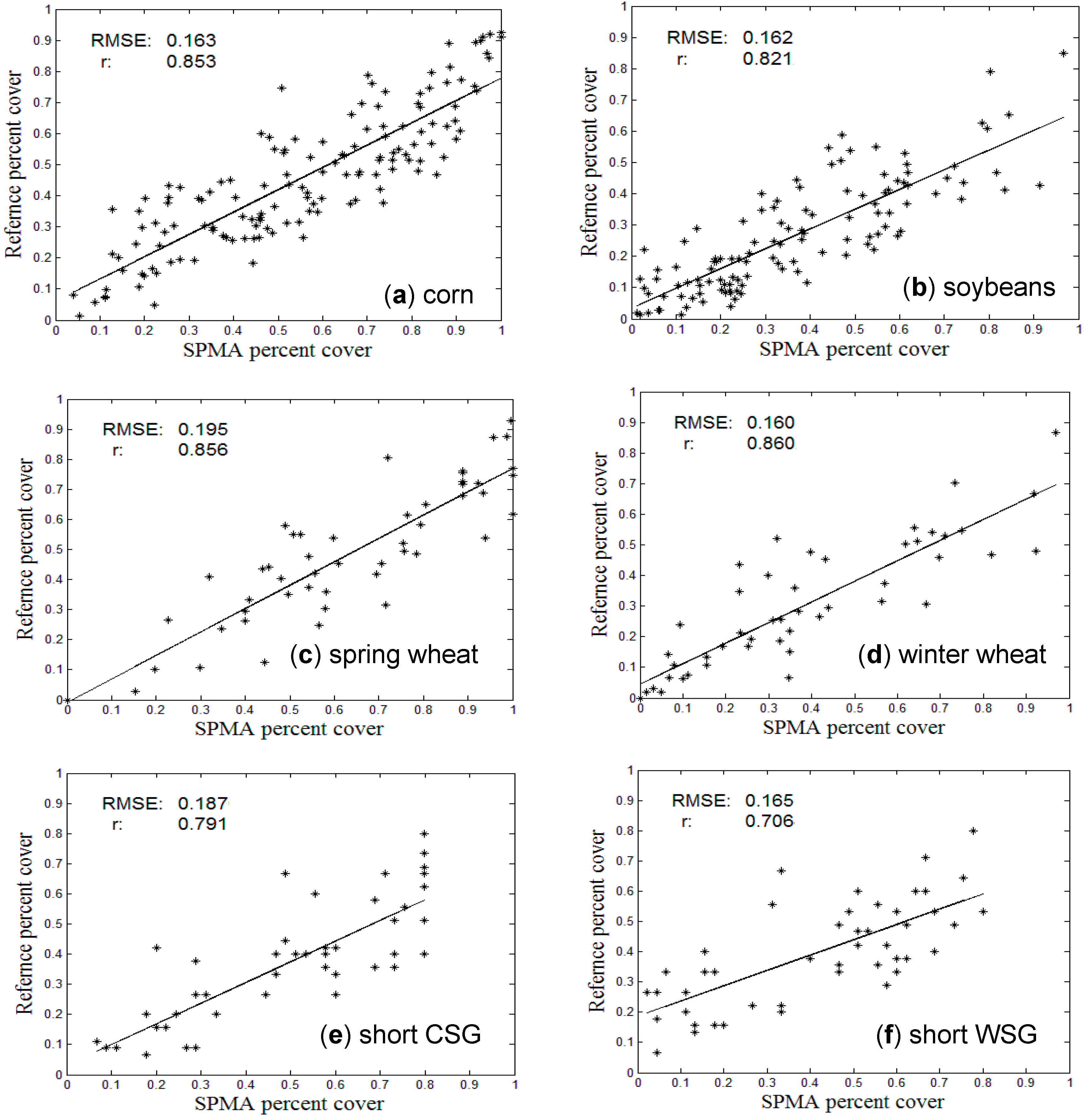
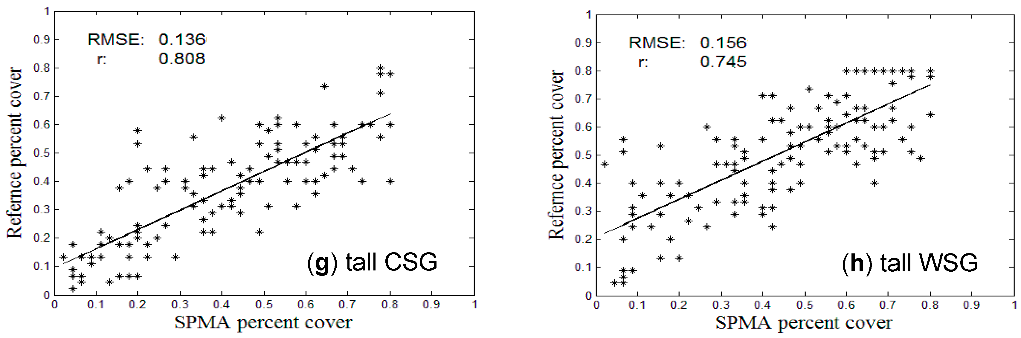
3.2. Comparison with References at Pixel Level

The SPMA-extracted crop percent covers were compared with the references from the CDL-summarized crop covers and published grass covers at sampled validation points. Table 2 lists the two accuracy measures for each crop. The RMSE values of all crops reached 14%–20%. When absolute errors were considered, all crops except tallgrass had negative SE values, indicating that the SPMA-extracted percent covers were generally higher than the CDL-summarized references. Tallgrass may be misclassified as corn and soybeans in the Corn Belt if there is a lack of training samples (pure pixels).
Table 2. Accuracy assessment of validation samples.
TypesCornSoybeanSpring WheatWinter WheatShort CSGShort WSGTall CSGTall WSG
RMSE0.1630.1620.1950.1600.1870.1650.1360.156
SE–0.096–0.099–0.152–0.081–0.124–0.0160.0490.059
Student’s t21.8421.3015.0811.528.976.548.377.52
When percent covers at all validation samples were considered (Figure 6), the Pearson’s correlation coefficients (r) in the scatterplots ranged from 0.706 to 0.860 for these crops, suggesting fair agreement between the SPMA-extracted and CDL-summarized percent covers. The relationships were statistically significant (p < 0.001) under the Student’s t test (degree of freedom = 149 for corn, soybeans, and tall grasses, and 49 for other crops). Table 2 also lists the Student’s t values of the test for all crops. Although all tests were significant, perennial crops had smaller t values than annual crops, which may be attributed to the uncertainties when their samples were extracted from the coarse-resolution grass abundance maps [15]. For annual crops (Figure 6(a–d)), the SPMA could effectively extract their percent covers in the lower end. In the higher end, however, the SPMA results turned out to be overestimated, because other crops (e.g., alfalfa, sorghum) and small plots of non-crop land covers were not considered in this study. For this reason, the correlation line was lower than the diagonal line in each plot. For perennial crops (Figure 6(e–h)), the references were from the ranked grass cover maps extracted from the MODIS time series. The points were more scattered in their scatterplots, but the RMSE reached similar values to those of annual crops.
Figure 6. The scatterplots between the SPMA-extracted percent covers (X-axis) and references (Y-axis) for the eight crops: corn (a), soybean (b), spring wheat (c), winter wheat (d), cool-season shortgrass (e), warm-season shortgrass (f), cool-season tallgrass (g), and warm-season tallgrass (h).
Remotesensing 07 00512 g006aRemotesensing 07 00512 g006b

3.3. Comparison with Crop Census Records at County Level
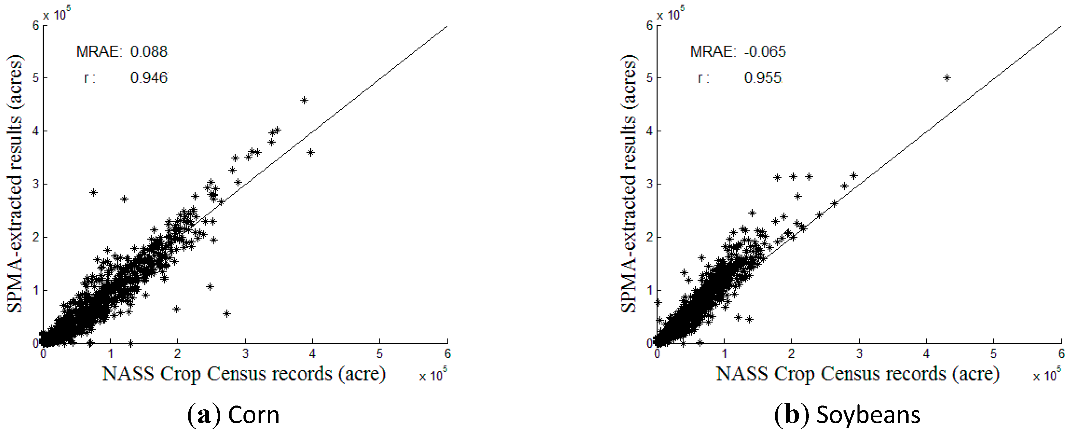
As the primary crops in the Midwest, corn and soybeans maintained good records of planting areas from the county-level NASS Crop Census data in 2007. To be comparable with these records, the pixel-level SPMA results were summarized into county-level crop planting acreages. The census records in a total of 1046 counties were extracted in the Midwest. Only corn and soybeans were compared. Other crops were not examined because spring wheat and winter wheat only grew in limited counties in the region. The warm-season and cool-season grasses were not specifically recorded in the census data.
Figure 7. The county-level comparison between the Crop Census records (X-axis) and the SPMA-extracted planting areas of corn (a) and soybeans (b).
Remotesensing 07 00512 g007
In Figure 7, the county-level comparison had a Pearson’s r of 0.946 for corn and 0.955 for soybeans, indicating high agreement between the SPMA results and the census records. The mean relative area errors (MRAE) reduced the uncertainties from county sizes and were quite low for both crops. For counties with corn planting areas higher than 300 k acres (Figure 7a), the SPMA estimations became much higher than those in the census records. For soybeans (Figure 7b), a majority of counties had their SPMA estimations higher than the census records, which resulted in a negative MRAE value of −0.065. Figure 7 agrees with the Crop Census and CDL products that soybean planting areas were lower than corn in most counties. When compared all over the region, the SPMA approach in this study extracted a similar range of the total corn planting area (93.99%) as the census records (Table 3). Soybean planting area was overestimated, and reached 116.91% of the census records.
Table 3. Accuracy assessment at county level.
TypesCounty LevelRegion-Level (Midwest)
MRAErSPMA Results (Million Acres)NASS Census (Million Acres)Ratio (SPMA/Census)
Corn0.0880.94672.29776.92193.99%
Soybean−0.0650.95561.61652.702116.91%
Regional agricultural monitoring requires large-area coverage of remotely sensed data and standardized image analysis. While the USDA CDL products are published annually and provide high-quality crop maps in the conterminous United States, the process involves a huge amount of medium-resolution satellite images and repeated classification and validation algorithms for individual states [4]. It is time-consuming and labor-intensive, and thus cannot meet the requirement of quick responses for regional or global studies. Coarse-resolution satellite sensors such as MODIS have the ability to make daily observations all over the globe. Although not suitable for crop mapping with individual scenes, time series of these data effectively reveal crop development throughout a growing season. In our recent study [30], the same set of MODIS time series was input to a Support Vector Machine (SVM) classifier to extract major crop types, especially bioenergy crops including corn and perennial native grass. The classification, however, was binary without considering the in-pixel mixed growth of crops. Although relatively high accuracies (~90%) were achieved using large CDL clusters as validation source, dominant crops were apparently overestimated at an expense of omission of small crop clusters in local areas. In comparison, this study addressed the mixed pixel problem in crop delineation. Our study extracted percent covers of major crops using an unmixing algorithm based on their unique phenological curves. While crop phenology may vary at different geographical locations, the spatially constrained endmember selection reduces these uncertainties by only considering endmembers in the local neighborhood. The randomly selected small-size CDL clusters (3 × 3 of the aggregated 500 m cells) provided a more explicit spatial representation of the validation source. An overall RMSE range of 14%–20% for all crops in the Midwest indicates the feasibility of our SPMA approach for fractional crop mapping with MODIS time series in major agricultural regions.
One advantage of our approach is the computation efficiency for regional mapping. With only four MODIS tiles covering the Midwest region, computation time of our study is significantly improved in comparison with hundreds of Landsat tiles in the same region that were processed in national products. The recent publications about data fusion between these multi-resolution images [31] may bring in further opportunities to improve the classification accuracies with multi-source satellite time series. Also, the 8-day, 250-m MODIS products (MOD09Q1 and MYD09Q1) have become available in recent years. At finer resolution than the 500-m imagery that we used in this study, these new datasets could have better SPMA results for regional crop mapping. One concern about the phenology-based analysis in this study rises from the uncertainties when only one-year satellite data were applied. The NDVI time series fairly reflects crop development cycles along the growing season. Its temporal variation, however, is highly influenced by seasonal weather conditions that vary year to year. It is less of a concern for annual crops in this study because our ground truth samples were extracted from CDL products in the same year. In areas where real-time truth data were not available (e.g., perennial grasses in this study), large uncertainties could be introduced during the endmember selection process of our SPMA approach. As our further research, multi-year time series will be explored to investigate these challenges, and to examine land use change in the long run.
Agricultural land use patterns are changing all over the world. With advanced biofuel demand, for example, corn planting expansion, environmental contamination, corn grain price increase, and food shortages are of increasing concern to sustainable agriculture in the U.S. Midwest. In our recent research [30], we performed phenology-assisted binary classifications of the MODIS time series in 2006–2008 to explore the corn boom in 2007, the year with the historical record for corn expansion. Multi-year satellite time series effectively identified this type of bioenergy land use change. By taking advantage of multi-crops in mixed pixels, fractional mapping conducted in this study provides more quantitative information for rapid assessment of crop planting areas, crop production, and land use conversion.

4. Conclusions

This study developed a spatially constrained phenology-assisted unmixing (SPMA) approach to extracting crop percent covers in the U.S. Midwest using MODIS time series in 2007. The NDVI time series of a pixel was assumed to be a linear combination of phenological curves from multiple crops in the pixel, and endmembers in a dynamic local neighborhood were selected in the unmixing process. The resulted spatial distributions of major crops agreed with the CDL products at randomly selected validation points, reaching an overall RMSE range of 14%–20% for all crops. The planting areas of major crops (corn and soybeans) also fit well with county-level Crop Census records in the region, although soybeans were slightly overestimated and corn underestimated in comparison with census data. In corn- and soybean-dominated counties (>300 k acres), the extracted acreages of both crops were higher than census data. With crop percent covers, the SPMA results verified the hypothesis of the spatial constraint and presented more spatial details of crop distributions from coarse-resolution satellite imagery. The SPMA approach developed in this study shows great potential for regional crop monitoring in U.S. agricultural lands. With multi-year satellite time series involved, it could provide spatially explicit information about the rapid growth of bioenergy land use for decision-making at a regional scale.

Acknowledgements

This research is supported by Agriculture and Food Research Initiative Competitive Grant (# 2012-67009-22137) from the USDA National Institute of Food and Agriculture. We thank the USDA NASS for publishing the CDL products and Crop Census records that serve as an excellent reference in this project.

Author Contributions

Cheng Zhong did the experiments and wrote the original manuscript. Cuizhen Wang supervised the process of data analysis and was responsible to manuscript revisions. Changshan Wu provided partial source codes for image analysis and offered valuable comments to the manuscript.

Conflicts of Interest

The authors declare no conflict of interest.

References

  1. 2007 Corn Crop A Record Breaker. Available online: http://www.nass.usda.gov/Newsroom/2008/01_11_2008.asp (accessed on 15 May 2014).
  2. Wang, C.; Fritschi, F.B.; Stacey, G.; Yang, Z. Phenology-based assessment of perennial energy crops in North American Tallgrass Prairie. Ann. Assoc. Am. Geogr. 2011, 101, 741–751. [Google Scholar] [CrossRef]
  3. Smith, W.K.; Cleveland, C.C.; Reed, S.C.; Miller, N.L.; Running, S.W. Bioenergy potential of the United States constrained by satellite observations of existing productivity. Environ. Sci. Tech. 2012, 46. [Google Scholar] [CrossRef]
  4. Boryan, C.; Yang, Z.; Mueller, R.; Craig, M. Monitoring US agriculture: The US department of agriculture, national agricultural statistics service, Cropland Data Layer Program. Geocarto Int. 2011, 26, 341–358. [Google Scholar] [CrossRef]
  5. Solomon, B.D.; Barnes, J.R.; Halvorsen, K.E. Grain and cellulosic ethanol: History, economics, and energy policy. Biomass Bioenerg. 2007, 31, 416–425. [Google Scholar] [CrossRef]
  6. Pittman, K.; Hansen, M.C.; Becker-Reshef, I.; Potapov, P.V.; Christopher, O.J. Estimating global cropland extent with multi-year MODIS data. Remote Sens. 2010, 2, 1844–1863. [Google Scholar] [CrossRef]
  7. Thenkabail, P.S.; Biradar, C.M.; Noojipady, P.; Dheeravath, V.; Li, Y.J.; Velpuri, M.; Gumma, M.; Reddy, G.P.O.; Turral, H.; Cai, X.L.; et al. Global Irrigated Area Map (GIAM), derived from remote sensing, for the end of the last millennium. Int. J. Remote Sens. 2009, 30, 3679–3733. [Google Scholar] [CrossRef]
  8. Thenkabail, P.S.; Hanjra, M.A.; Dheeravath, V.; Gumma, M.A. A holistic view of global croplands and their water use for ensuring global food security in the 21st century through advanced remote sensing and non-remote sensing approaches. Remote Sens. 2010, 2, 211–261. [Google Scholar] [CrossRef] [Green Version]
  9. Santos, U.L. Spectral identification of native and non-native plant species. In Proceedings of ASD and IEEE GRS; Art, Science and Applications of Reflectance Spectroscopy Symposium, Boulder, CO, USA, 23–25 February 2010.
  10. Xie, Y.; Sha, Z.; Yu, M. Remote sensing imagery in vegetation mapping: A review. J. Plant Ecol. 2008, 1, 9–23. [Google Scholar] [CrossRef]
  11. McCloy, K.R.; Lucht, W. Comparative evaluation of seasonal patterns in long time series of satellite image data and simulations of a global vegetation model. IEEE Trans. Geosci. Remote Sens. 2004, 42, 140–153. [Google Scholar] [CrossRef]
  12. Wang, C.; Jamison, B.; Spicci, A. Trajectory-based warm season grass mapping in Missouri prairies with multi-temporal ASTER imagery. Remote Sens. Environ. 2010, 114, 531–439. [Google Scholar] [CrossRef]
  13. Peterson, D.L.; Price, K.P.; Martinko, E.A. Discriminating between cool season and warm season grassland cover types in Northeaster Kansas. Int. J. Remote Sens. 2002, 23, 5015–5030. [Google Scholar] [CrossRef]
  14. Wardlow, B.D.; Egbert, S.L.; Kastens, J.H. Analysis of time-series MODIS 250 m vegetation index data for crop classification in the U.S. Central Great Plains. Remote Sens. Environ. 2007, 108, 290–310. [Google Scholar] [CrossRef]
  15. Wang, C.; Hunt, E.R.; Zhang, L.; Guo, H. Phenology-assisted classification of C3 and C4 grasses in the U.S. Great Plains and their climate dependency with MODIS time series. Remote Sens. Environ. 2013, 138, 90–101. [Google Scholar] [CrossRef]
  16. Homer, C.; Huang, C.; Yang, L.; Wylie, B.; Coan, M. Development of a 2001 national landcover database for the United States. Photogramm. Eng. Remote Sens. 2004, 70, 829–840. [Google Scholar] [CrossRef]
  17. Geerken, R.A. An algorithm to classify and monitor seasonal variations in vegetation phenologies and their inter-annual change. ISPRS J. Photogramm. Remote Sens. 2009, 64, 422–431. [Google Scholar] [CrossRef]
  18. Wardlow, B.D.; Egbert, S.L. Large-area crop mapping using time-series MODIS 250 m NDVI data: An assessment for the US Central Great Plains. Remote Sens. Environ. 2008, 112, 1096–1116. [Google Scholar] [CrossRef]
  19. Lobell, D.B.; Asner, G.P. Cropland distributions from temporal unmixing of MODIS data. Remote Sens. Environ. 2004, 93, 412–422. [Google Scholar] [CrossRef]
  20. Weng, Q.; Hu, X.; Lu, D. Extracting impervious surface from medium spatial resolution multispectral and hyperspectral imagery: A comparison. Int. J. Remote Sens. 2008, 29, 3209–3232. [Google Scholar] [CrossRef]
  21. Weng, Q. Remote sensing of impervious surfaces in the urban areas: Requirements, methods, and trends. Remote Sens. Environ. 2012, 117, 34–49. [Google Scholar] [CrossRef]
  22. Deng, C.; Wu, C. A spatially adaptive spectral mixture analysis for mapping subpixel urban impervious surface distribution. Remote Sens. Environ. 2013, 133, 62–70. [Google Scholar] [CrossRef]
  23. Busetto, L.; Meroni, M.; Colombo, R. Combining medium and coarse spatial resolution satellite data to improve the estimation of sub-pixel NDVI time series. Remote Sens. Environ. 2008, 112, 118–131. [Google Scholar] [CrossRef]
  24. Ozdogan, M. The spatial distribution of crop types from MODIS data: Temporal unmixing using independent component analysis. Remote Sens. Environ. 2010, 114, 1190–1204. [Google Scholar] [CrossRef]
  25. Somers, B.; Asner, G.P.; Tits, L.; Coppin, P. Endmember variability in spectral mixture analysis: A review. Remote Sens. Environ. 2011, 115, 1603–1616. [Google Scholar] [CrossRef]
  26. Ethanol Facilities’ Capacity by State. Available online: http://www.neo.ne.gov/statshtml/121.htm. (accessed on 15 May 2014).
  27. Savitzky, A.; Golay, M.J.E. Smoothing and differentiation of data by simplified least squares procedures. Anal. Chem. 1964, 36, 1627–1639. [Google Scholar] [CrossRef]
  28. Cropland Layer Data. Available online: http://nassgeodata.gmu.edu/CropScape/ (accessed on 15 May 2014).
  29. Hu, X.; Weng, Q. Estimating impervious surfaces from medium spatial resolution imagery using the self-organizing map and multi-layer perceptron neural networks. Remote Sens. Environ. 2009, 113, 2089–2102. [Google Scholar] [CrossRef]
  30. Wang, C.; Zhong, C.; Yang, Z. Assessing bioenergy-driven agricultural land use change and biomass quantities in the U.S. Midwest with MODIS time series. J. Appl. Remote Sens. 2014, 8. [Google Scholar] [CrossRef]
  31. Zhu, X.; Cheng, J.; Gao, F.; Chen, X.; Masek, J.G. An enhanced spatial and temporal adaptive reflectance fusion model for complex heterogeneous regions. Remote Sens. Environ. 2010, 114, 2610–2623. [Google Scholar] [CrossRef]

