
High-Precision Attitude Post-Processing and Initial Verification for the ZY-3 Satellite


Abstract
:1. Introduction
2. Methodology
2.1. Principle
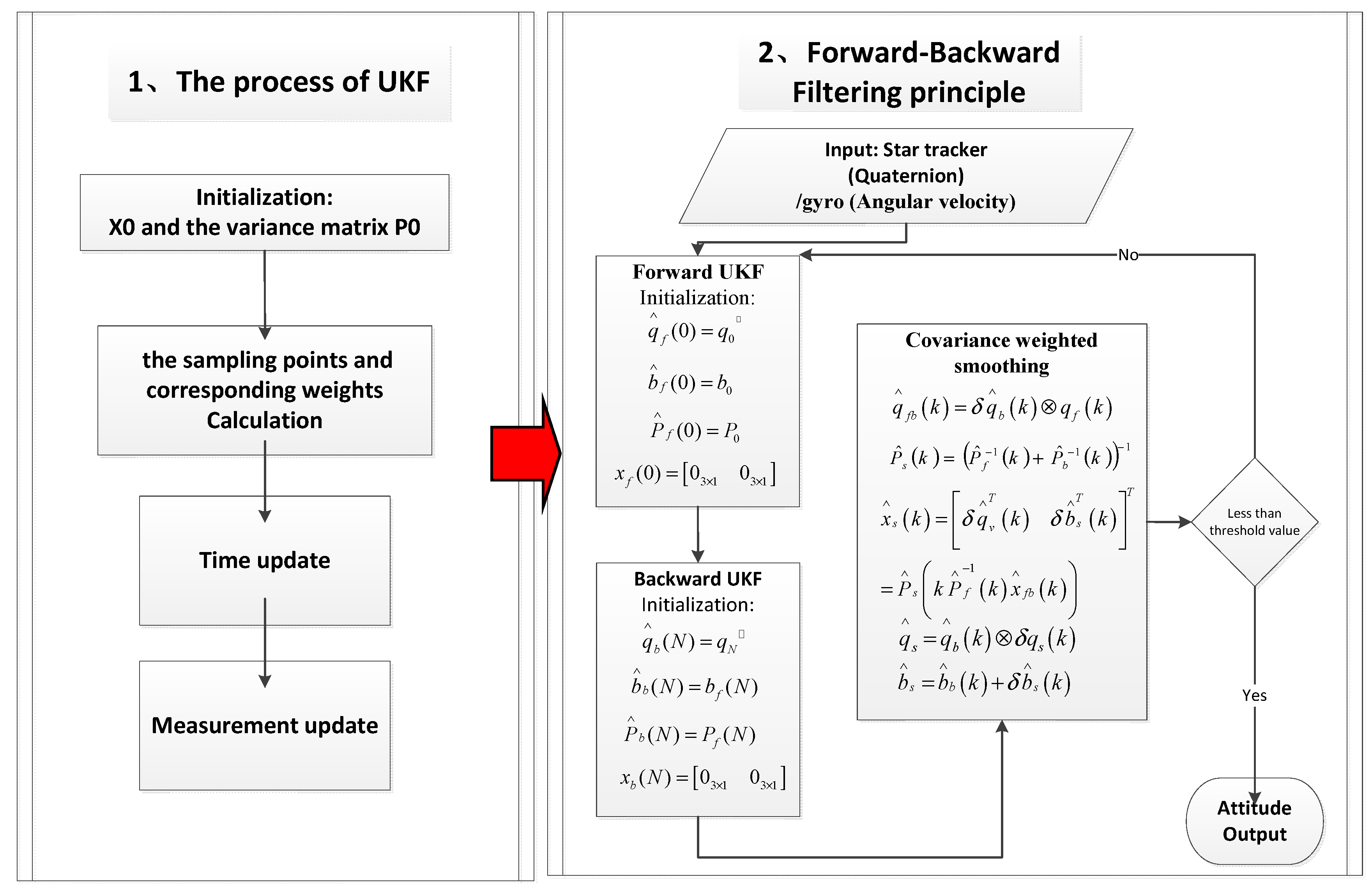
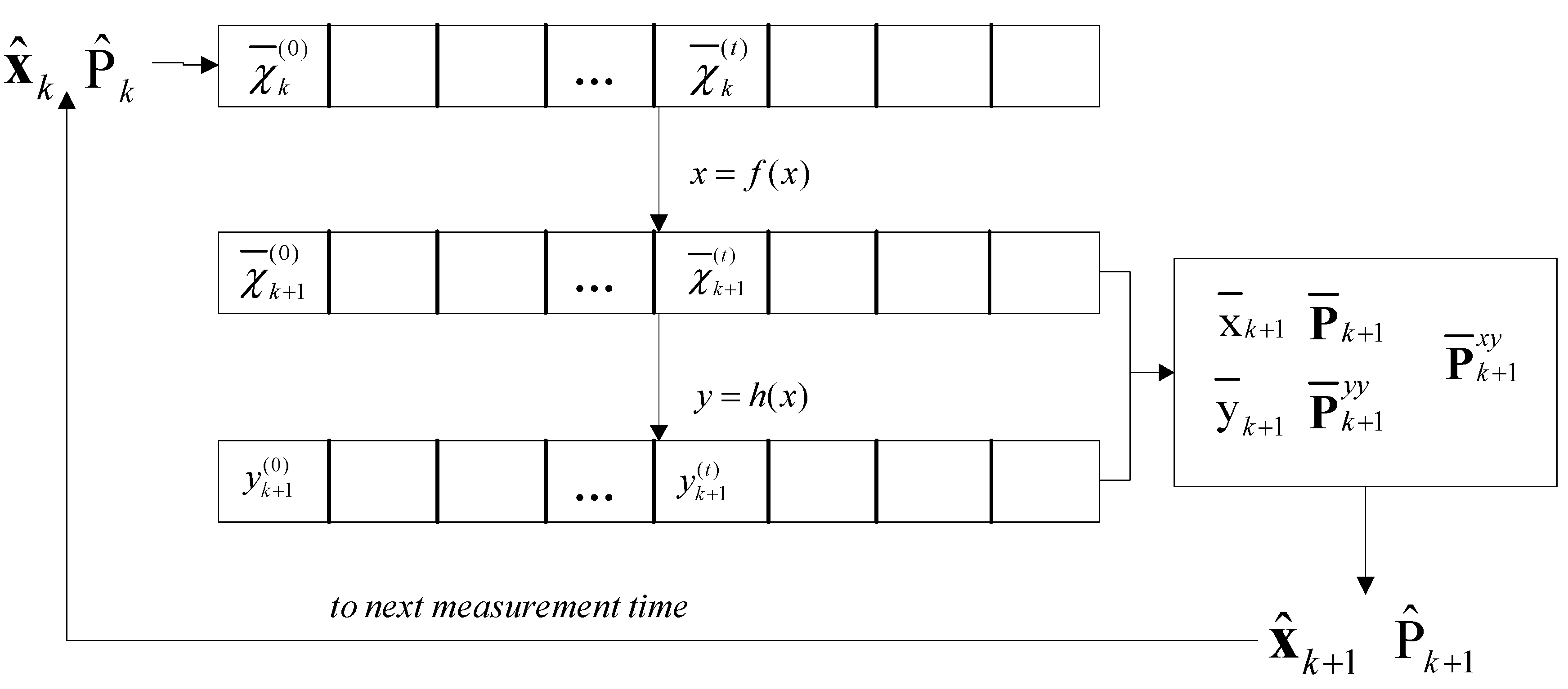
2.1.1. The UKF Filtering Process


2.1.2. Forward-Backward Filtering Strategy
 at thelast measurement epoch tN, and the initial estimated value of the gyro bias and error covariance are obtained from the forward filtering results.
2.2. Workflow

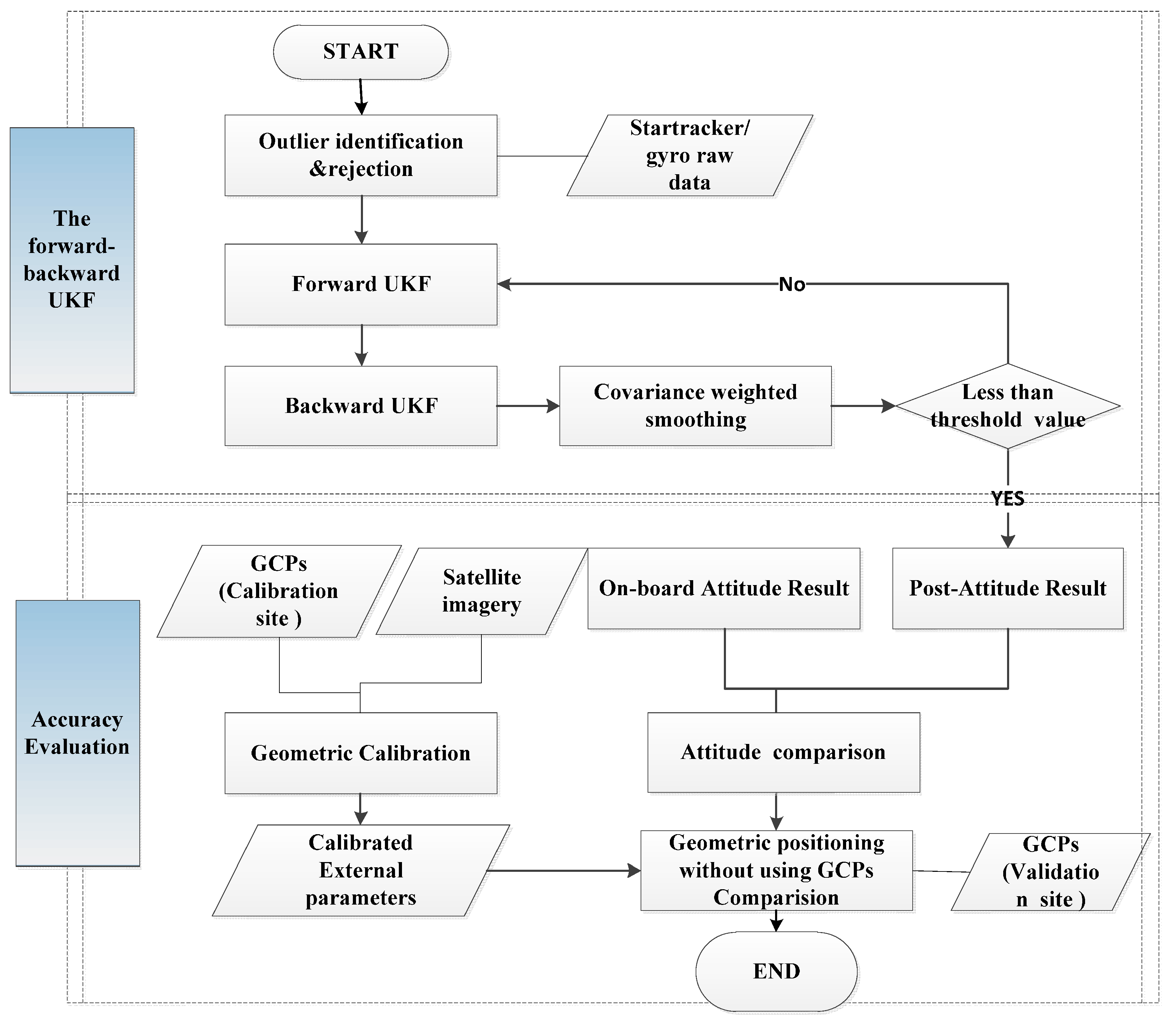
2.2.1. The Forward-Backward Filtering for Attitude Post-Processing
- (1)
- Outlier identification for the unpacked raw star tracker/gyro data. For the raw gyro data: firstly, determine whether the gyro output exceeds the measurement range. If yes, the gyro output is judged as outlier. If not, the angle increment output of gyro output in current period should be compared with that in the last period, these output would be considered as outliers when the measured angle increment is larger than the theoretical value. For those raw star tracker data: transform the star tracker output (quaternion) to the measurement direction vectors defined in the optical axis and horizontal axis, and then fit these vectors using a polynomial approach. If the deviation of the measured and fitted values is larger than the threshold value, the measured values will be considered as outliers and excluded.
- (2)
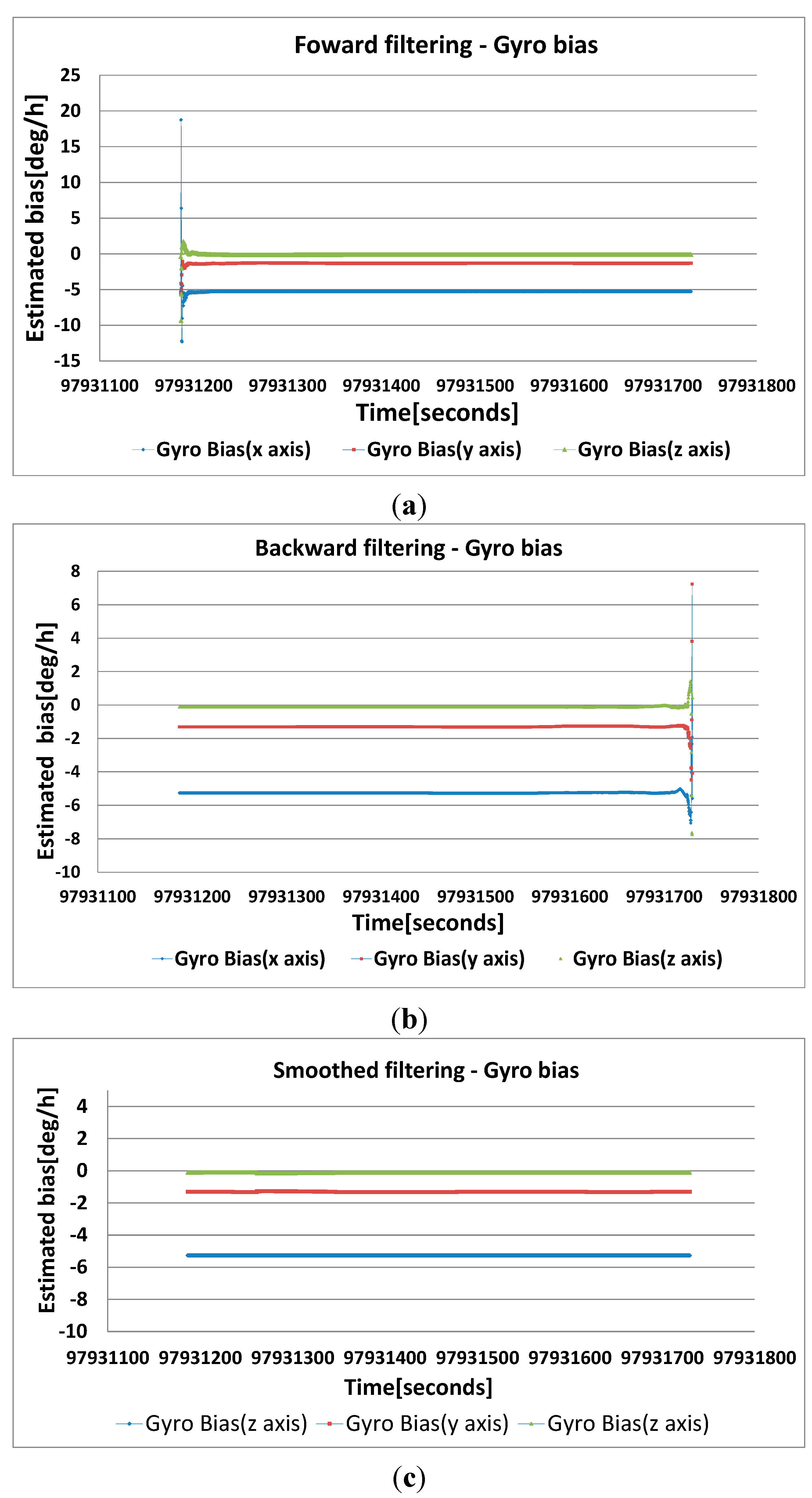
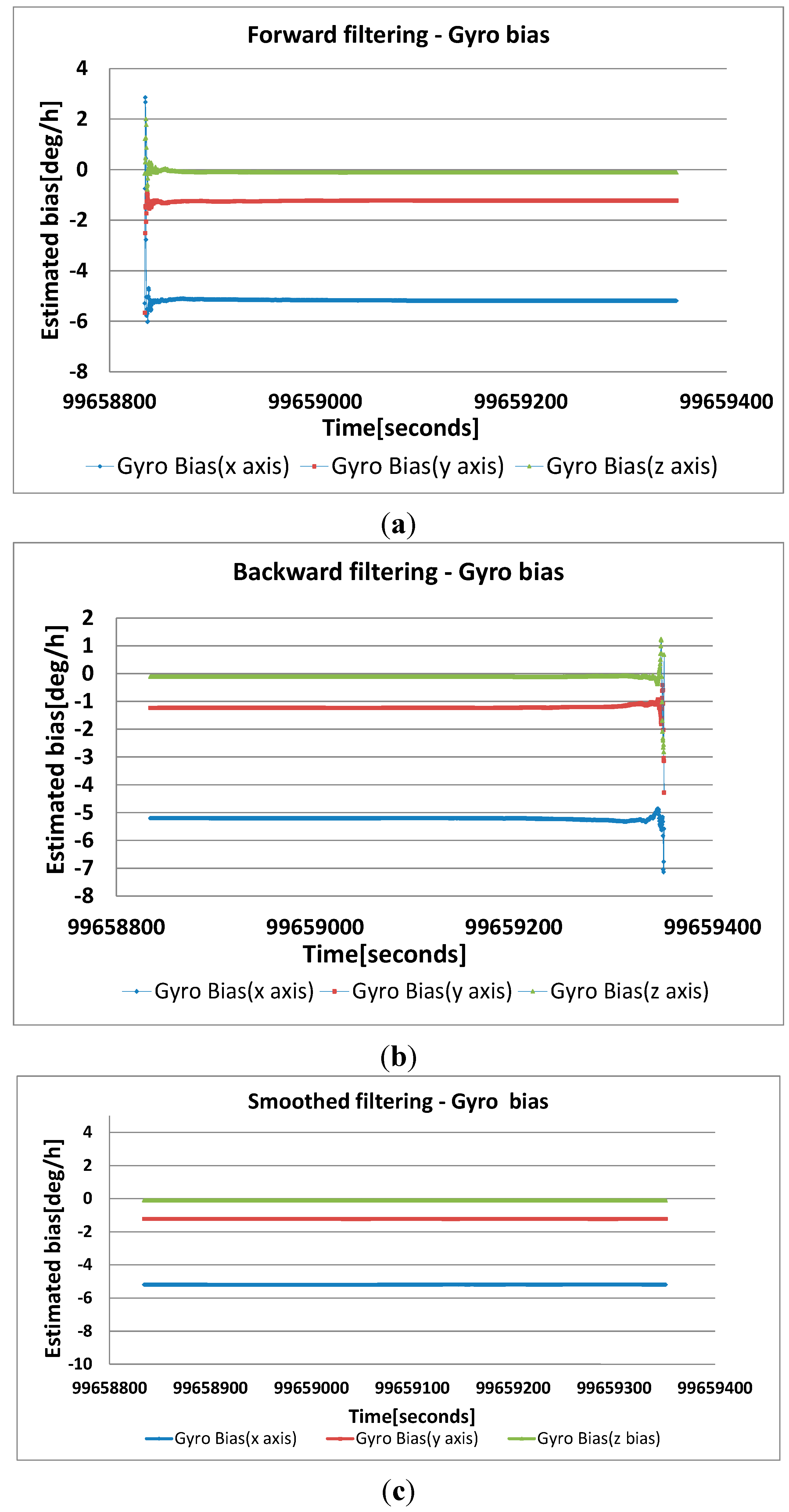
- Determine the initial estimated in the forward UKF by the dual-vector attitude determination method with the initial output of two star trackers [35], and set the initial value of the state variable and gyro bias using Equations (17) and (18). The initial gyro bias of the real-time processing result is recorded and transferred to a ground station. The sampling points and corresponding weights are obtained by Equations (4)–(6). The error covariance sets an empirical value by analyzing the real-time measurement results. The time and measurement are updated by Equations (7)–(14). Once the state vector at epoch tk is calculated with Equation (13), the estimated quaternion and gyro biases at epoch tk are updated by Equations (15) and (16).
- (3)
- The backward filtering is implemented from time tN to t0 with decreasing time. The initial value is obtained by the dual-vector determination with the two star trackers’ output at the last measurement epoch tN. The initial value of the gyro bias and error covariance can bedirectly obtained from the forward filtering results. All initial values are set by Equations (19) and (20).Similarly, the time and measurement are updated by Equations (7)–(14).Once the state vector is calculated by using Equation (13), the estimated quaternion and gyro biases at the epoch tk are updated by Equations (15) and (16).
- (4)
- Record the covariance and in the forward and backward filtering processes, and calculate the smoothing covariancefrom Equation (22). The smoothing state variables can be calculated by Equation (23); then, the smoothing estimated values of and can be updated by Equations (24) and (25). The previous and current RMS values of the observation residuals are calculated from Equation (27). A pre-set value is set to . If the difference between the new RMS and old RMS is less than , then the iteration process stops.
2.2.2. Attitude Accuracy Comparison and Evaluation
- (1)
- Construct a rigorous geometric imaging model of the ZY-3 satellite, as shown in Equation (28).This imaging model borrows concepts from SPOT-5 [36], and it is sufficiently validated [37,38].where
![Remotesensing 07 00111 i004]() ,
, ![Remotesensing 07 00111 i005]() are the line-of-sight vectors for each CCD detector in the camera’s coordinate system [39], i.e., “the internal parameters”. is a transformation matrix of the alignment angles between the satellite and the camera, i.e., “the external parameters”. is the transformation matrix from the J2000 coordinate system to the WGS84 coordinate system. is the attitude transformation matrix from the satellite body coordinate system to the J2000 coordinate system.
is the position of the projection center in the WGS84 coordinate system that is obtained by orbit position post-processing technology using the raw GPS data; the post-processing accuracy of ZY-3 is superior to 5 cm. represents the geographic coordinates of the ground object in WGS84.
are the line-of-sight vectors for each CCD detector in the camera’s coordinate system [39], i.e., “the internal parameters”. is a transformation matrix of the alignment angles between the satellite and the camera, i.e., “the external parameters”. is the transformation matrix from the J2000 coordinate system to the WGS84 coordinate system. is the attitude transformation matrix from the satellite body coordinate system to the J2000 coordinate system.
is the position of the projection center in the WGS84 coordinate system that is obtained by orbit position post-processing technology using the raw GPS data; the post-processing accuracy of ZY-3 is superior to 5 cm. represents the geographic coordinates of the ground object in WGS84. - (2)
- The step calibration method is adopted for ZY-3’s in-flight geometric calibration[40,41,42,43].A reference image is simulated with a large-scale DOM/DEM if the satellite attitude and orbit data are given; then, the simulated image is resampled to the same resolution as the ZY-3 image. Phase correlation is employed for the image registered between the ZY-3 image and the simulated reference image to obtain many dense reference points along and across the track of the ZY-3 image [43]. The sequential solution method is used to calculate
![Remotesensing 07 00111 i004]() ,
, ![Remotesensing 07 00111 i005]() and with Equation (28). Certainly, if (
and with Equation (28). Certainly, if ( ![Remotesensing 07 00111 i004]() ,
, ![Remotesensing 07 00111 i005]() ) of all CCD are known, then can be directly calibrated by Equation (28) using GCPs.
) of all CCD are known, then can be directly calibrated by Equation (28) using GCPs. - (3)
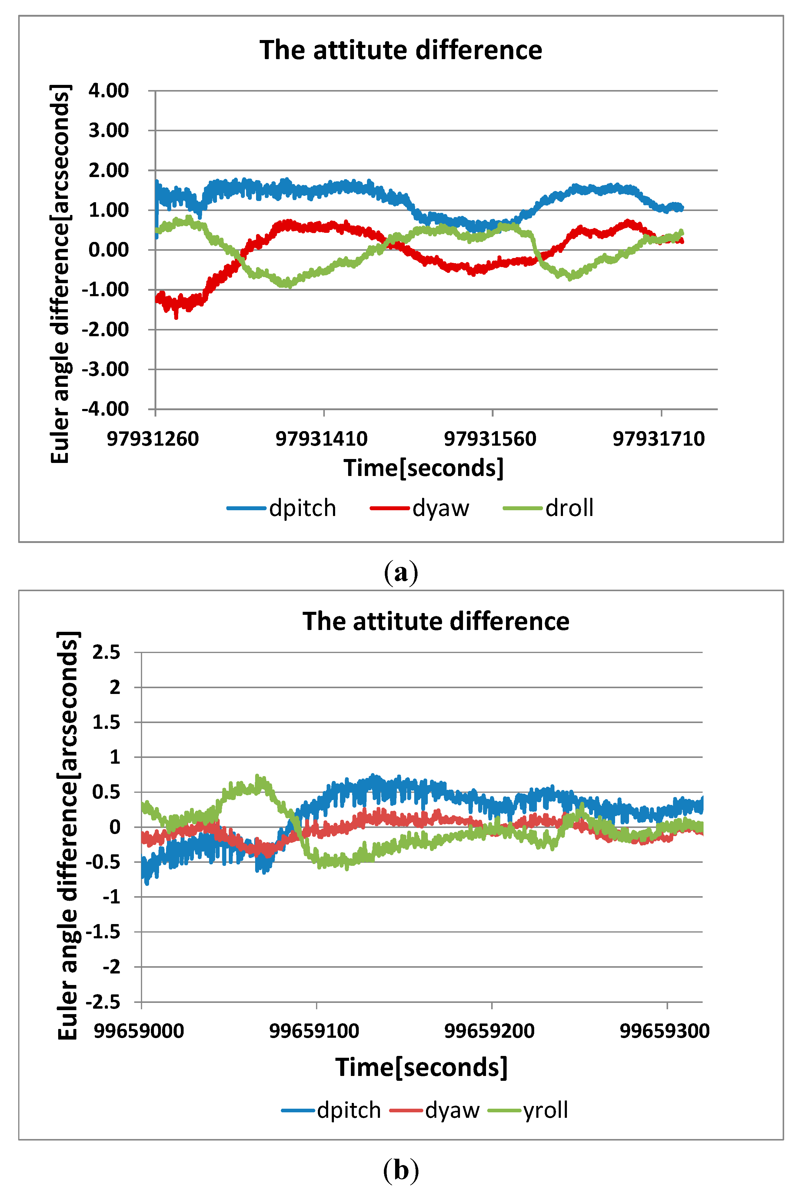
- According to the equivalent relationship between the attitude matrix and the attitude quaternion, along with quaternion theory [44], the difference between the on-board and post-processed attitudes can be calculated by , where denotes the post-processed attitude, and q denotes the on-board attitude. The quaternion deviation ∆q can be transformed to the Euler angle defined in J2000 [45,46]. , , .
- (4)
- Collect the ZY-3 stereo images (forward-view, nadir-view and backward-view) that cover the verification site, and obtain the image coordinates of homonymy points in the stereo images by image registration or artificial pricking. Suppose, and are the image coordinates of one GCP in the forward-view, nadir-view and backward-view images, respectively. Assume that x is the flight direction and y is the CCD direction. For the forward-view image, the attitude and position information of is interpolated with the imaging time, and the CCD detector of
![Remotesensing 07 00111 i006]() is interpolated by the calibrated internal parameters. Similarly, the attitude and orbit data of this GCP in the other views are also obtained. The object space coordinate of the GCP can be calculated by Equation (28).The difference between the calculated and the known of this GCP is computed, and the RMS of the difference is used to evaluate the accuracy.
is interpolated by the calibrated internal parameters. Similarly, the attitude and orbit data of this GCP in the other views are also obtained. The object space coordinate of the GCP can be calculated by Equation (28).The difference between the calculated and the known of this GCP is computed, and the RMS of the difference is used to evaluate the accuracy.


3. Experiment Data and Analysis of the Results
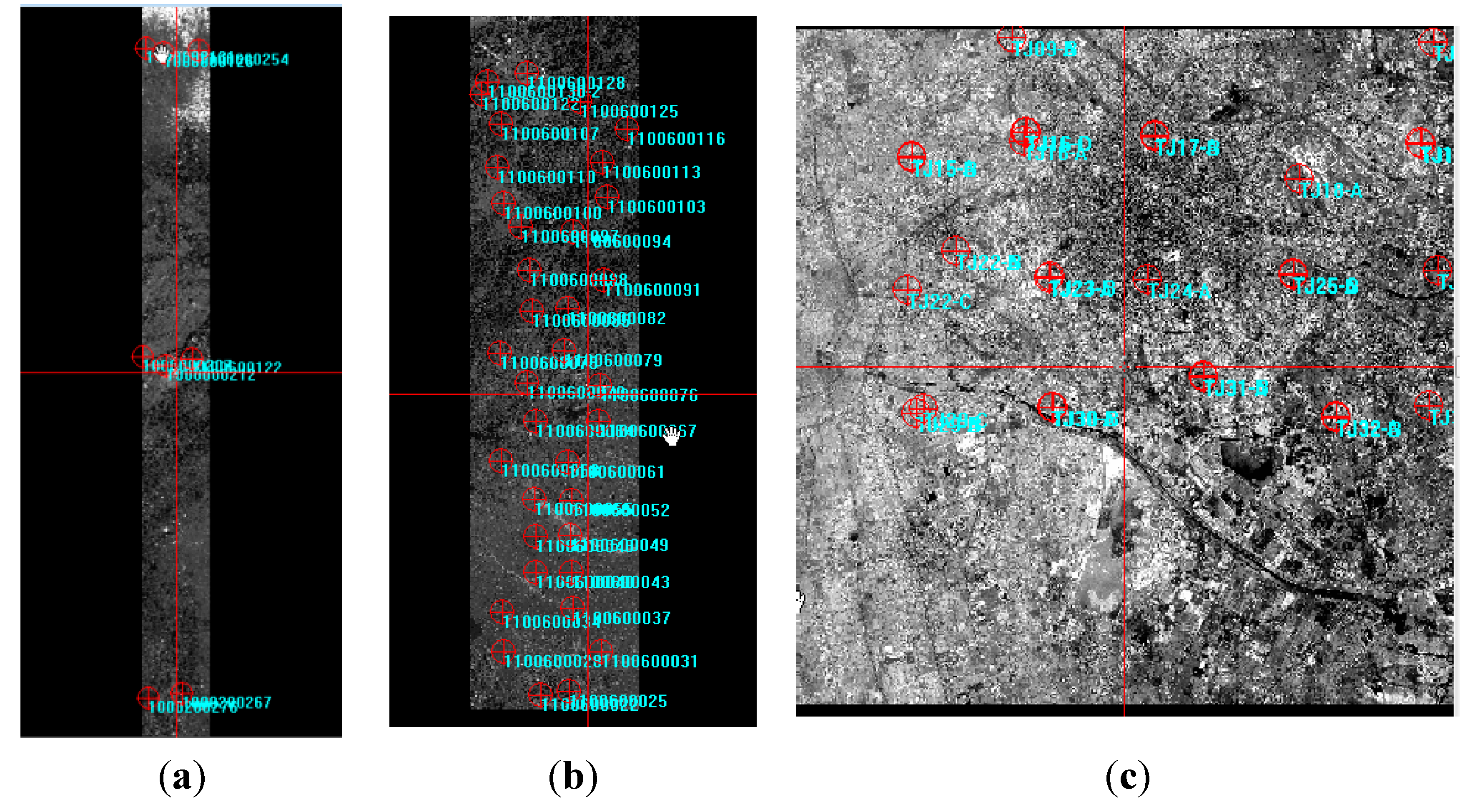
3.1. Data Preparation

| Test Site | Image Acquisition Date | Track Number | Image Path/Row | Number of GCPs | Distribution | Terrain |
|---|---|---|---|---|---|---|
| Taiyuan (calibration) | 3 February 2012 | 381 | Ten scenes: 6/120~6/129 | 8 | well-distributed | Mountain |
| Taihang(validation) | 8 February 2012 | 457 | Six scenes: 5/120~5/125 | 36 (checkpoints) | well-distributed | Mountain |
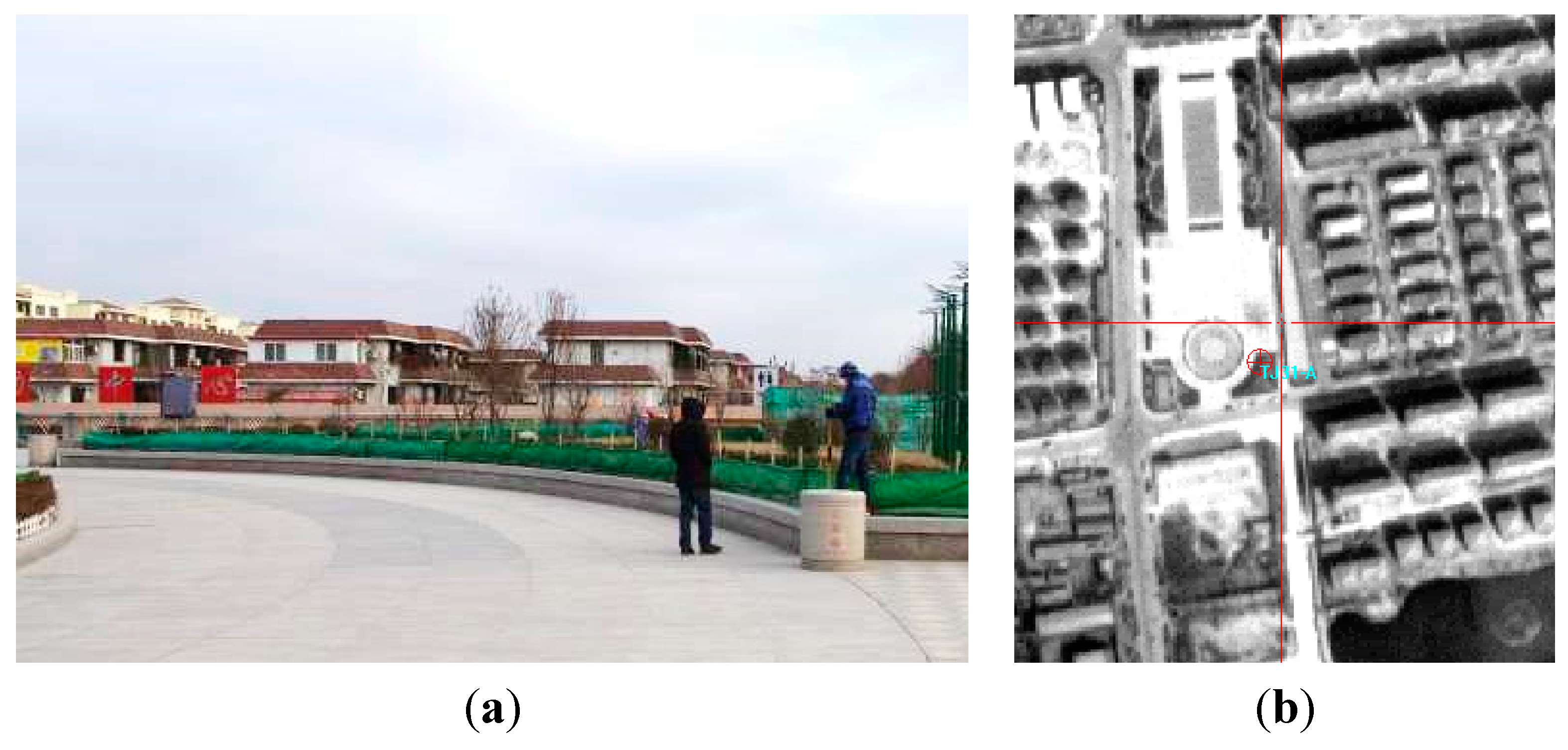
| Tianjin (validation) | 28 February 2012 | 785 | One scene: 896/127 | 22 (checkpoints) | well-distributed | Plain |


3.2. Results and Discussion
3.2.1. The Post-Processed Results and Comparison with the On-Board Attitudes
| Camera | Three Axis Angle (Units: Radian) | ||
|---|---|---|---|
| f | w | k | |
| BWD | 0.0024873321 | 0.0017746478 | 0.0028587395 |
| NAD | 0.0005171015 | 0.0017320041 | 0.0037815675 |
| FWD | 0.0018654008 | 0.0017649895 | 0.0030016442 |
| Geographical Coordinate | ----- | Minimum (m) | Maximum (m) | RMSE (m) |
|---|---|---|---|---|
| X | Before calibration | 52.783 | 63.438 | 58.028 |
| After calibration | 0.227 | 5.714 | 3.355 | |
| Y | Before calibration | 37.166 | 31.135 | 34.258 |
| After calibration | 0.071 | 2.818 | 2.031 | |
| Z | Before calibration | 0.570 | 6.722 | 3.605 |
| After calibration | −0.142 | −3.446 | 2.165 |


3.2.2. Evaluation and Comparison of the Attitude Accuracy
| Geographical Coordinate | Attitude | Minimum (m) | Maximum (m) | RMSE (m) |
|---|---|---|---|---|
| X | On-board | 4.009 | 12.147 | 8.080 |
| Post-processed | 2.750 | 11.070 | 7.107 | |
| Y | On-board | 7.010 | 15.466 | 12.27 |
| Post-processed | 6.425 | 14.671 | 11.57 | |
| Z | On-board | 0.729 | 7.315 | 3.633 |
| Post-processed | 0.138 | 6.290 | 3.631 | |
| (a) | ||||
| Geographical Coordinate | Attitude | Minimum (m) | Maximum (m) | RMSE (m) |
| X | On-board | 9.485 | 13.025 | 11.465 |
| Post-processed | 8.618 | 11.914 | 10.311 | |
| Y | On-board | 0.096 | 3.863 | 2.294 |
| Post-processed | 0.057 | 2.125 | 1.191 | |
| Z | On-board | 6.903 | 13.117 | 9.796 |
| Post-processed | 3.517 | 10.728 | 6.796 | |
| Image Coordinate | Attitude | Minimum (Pixel) | Maximum (Pixel) | RMSE (Pixel) |
|---|---|---|---|---|
| X | On-board | 0.003 | 2.450 | 0.735 |
| Post-processed | 0.002 | 2.295 | 0.682 | |
| Y | On-board | 0.001 | 1.657 | 0.382 |
| Post-processed | 0.000 | 1.537 | 0.361 | |
| XY | On-board | 0.006 | 2.533 | 0.828 |
| Post-processed | 0.005 | 2.449 | 0.772 | |
| (a) | ||||
| Image Coordinate | Attitude | Minimum (Pixel) | Maximum (Pixel) | RMSE (Pixel) |
| X | On-board | 0.019 | 4.097 | 1.706 |
| Post-processed | 0.004 | 3.501 | 1.113 | |
| Y | On-board | 0.001 | 3.360 | 0.701 |
| Post-processed | 0.000 | 3.026 | 0.564 | |
| XY | On-board | 0.060 | 4.681 | 1.797 |
| Post-processed | 0.014 | 4.400 | 1.315 | |
4. Conclusions
Acknowledgments
Author Contributions
Conflicts of Interest
References
- Dial, G.; Bowen, H.; Gerlach, F.; Grodecki, J.; Oleszczuk, R. IKONOS satellite, imagery, and products. Remote Sens. Environ. 2003, 88, 23–36. [Google Scholar]
- Tang, X.; Xie, J.; Zhang, G. Development and status of mapping satellite technology. Spacecr. Recovery Remote Sens. 2012, 33, 17–20. [Google Scholar]
- Kalman, R.E. A new approach to linear filtering and prediction problem. J. Basic Eng. 1960, 82, 95–108. [Google Scholar]
- Speyer, J. Computation and transmission requirements for a decentralized linear-quadratic-Gaussian control problem. IEEE Trans. Autom. Control. 1979, 24, 266–269. [Google Scholar]
- Kerr, T. Decentralized filtering and redundancy management for multi-sensor navigation. IEEE Trans. Aerosp. Electron. Syst. 1987, 23, 83–119. [Google Scholar]
- Calson, N.A.; Berarducci, M.P. Federated Kalman filter simulation results. Navigation 1994, 41, 297–321. [Google Scholar]
- Anderson, B.D.O.; Moore, J.B. Optimal Filtering; Prentice-Hall: Englewood Cliffs, NJ, USA, 1979. [Google Scholar]
- Psiaki, M.L. Attitude determination filtering via extended quaternion estimation. J. Guid. Control Dyn. 2000, 23, 206–214. [Google Scholar]
- Rtliter, A.H.J.D.; Damaren, C.J. Extended Kalman Filtering and nonlinear predictive filtering for spacecraft attitude determination. Can. Aeronaut. Space J. 2002, 48, 13–23. [Google Scholar]
- Lefebvre, T.; Bruyninckx, H.; Schutter, J.D. Kalman filters for nonlinear systems: A comparison of performance. Int. J. Control. 2004, 77, 639–653. [Google Scholar]
- Jerry, M.M. Lessons in Estimation Theory for Signal Processing, Communications and Control; Prentice Hall: Upper Saddle River, NJ, USA, 2005. [Google Scholar]
- Kaminski, P.; Bryson, A.; Schmidt, S. Discrete square root filtering: A survey of current techniques. IEEE Trans. Autom. Control. 1971, 16, 727–736. [Google Scholar]
- Hammarling, S. A Survey of Numerical Aspects of Plane Rotations. Available online: http://www.maths.manchester.ac.uk/~sven/pubs/mddx.pdf (accessed on 18 November 2014).
- Wang, H.; Gregory, R. On the reduction of an arbitrary real square matrix to tridiagonal form. Math. Comput. 1964, 87, 501–505. [Google Scholar]
- Chandrasekar, J.; Kim, I.S.; Bernstein, D.S.; Ridley, A.J. Choleskyesky-based reduced-rank Square-Root Kalman filtering. In Proceedings of the 2008 American Control Conference (ACC), Seattle, WA, USA, 11–13 June 2008; pp. 3987–3992.
- Bierman, G.J. Measurement updating using the U-D factorization. In Proceedings of the 1975 IEEE Conference on Decision and Control, Houston, TX, USA, 10–12 December 1975; pp. 337–346.
- Julier, S.J.; Uhlmann, J.K. A new extension of the Kalman filter to nonlinear system. In Proceedings of the 11th International Symposium on Aerospacel/Defence Sensing, Simulation and Controls, Orlando, FL, USA, 21 April 1997.
- Julier, S.J. The scaled unscented transformation. In Proceedings of the 2002 American Control Conference, Anchorage, AK, USA, 8–10 May 2002; pp. 4555–4559.
- Crassidis, J.L.; Markley, F.L. Unscented filtering for spacecraft attitude estimation. Am. Inst. Aeronaut. Astronaut. 2003, 26, 536–542. [Google Scholar]
- Julier, S.J.; Durrant-whyte, H.F. Process models for the high-speed navigation of road vehicles. In Proceedings of the 1995 International Conference on Robotics and Automation (ICRA), Nagoya, Japan, 21–27 May1995; pp. 101–105.
- Wan, E.A.; Merve, R. The unscented Kalman filter for nonlinear estimation. In Proceedings of the 2000 IEEE Adaptive Systems for Signal Processing, Communications, and Control Symposium, AS-SPCC, Lake Louise, AB, Canada, 1–4 October 2000; pp. 153–158.
- Merve, R.; Wan, E.A. The square-root unscented Kalman filter for state and parameter-estimation. In Proceedings of the 2001 International Conference on Acoustics, Speech, and Signal Processing, Salt Lake City, UT, USA, 7–11 May 2001; pp. 3461–3464.
- Burello, M. SPOT1 In-Orbit Attitude Control System Performances. In Proceedings of the 1987 AAS Guidance and Control Conference, Keystone, CO, USA, 4–8 February 1987.
- Grodecki, J.; Dial, G. IKONOS geometric accuracy validation. ISPRS Arch. 2002, 34, 50–55. [Google Scholar]
- Mulawa, D. On-orbit geometric calibration of the OrbView-3 high resolution imaging satellite. ISPRS Arch. 2004, 35, 1–6. [Google Scholar]
- Rauch, H.E.; Tung, F.C.; Striebel, T. Maximum likelihood estimates of linear dynamic system. Am. Inst. Aeronaut. Astronaut. 1965, 80, 1445–1450. [Google Scholar]
- Sarkka, S. Unscented rauch-tung-striebel smoother. IEEE Trans. Autom. 2008, 53, 845–849. [Google Scholar]
- Takanori, I. Precision attitude and position determination for Advanced Land Observing Satellite (ALOS). Proc. SPIE 2009, 34, 1845–1848. [Google Scholar]
- Department of the Interior U.S. Geological Survey. Landsat 7 Image Assessment System (IAS) Geometric Algorithm Theoretical Basis Document. Available online: http://landsat.usgs.gov/documents/LS-IAS-01_Geometric_ATBD.pdf (accessed on 19 November 2014).
- Sungkoo, B. GLAS Spacecraft Attitude Determination Using CCD Star Tracker and 3-Axis Gyros. Ph.D. Thesis, the University of Texas at Austin, Austin, TX, USA, 1998. [Google Scholar]
- Li, D. China’s First Civilian Three-line-array Stereo mapping satellite: ZY-3. Acta. Geod. Cartogr. Sin. 2012, 41, 317–322. [Google Scholar]
- Tang, X.; Xie, J. Overview of the key technologies for high-resolution satellite mapping. Int. J. Digit. Earth 2012, 5, 227–240. [Google Scholar]
- Vallado, D.A. General perturbation techniques. In Fundamentals of Astro dynamics and Applications, 2nd ed.; Kluwer Academic Publishers: Dordrecht, The Netherlands, 2001; pp. 707–713. [Google Scholar]
- Tapley, B.D.; Schutz, B.E.; Born, G.H. Fundamentals of orbit determination. In Statistical Orbit Determination; Elsevier Academic Press: Waltham, MA, USA, 2004; pp. 159–284. [Google Scholar]
- Bar-Itzhack, I.Y.; Harman, R.R. Optimized TRIAD algorithm for attitude determination. Am. Inst. Aeronaut. Astronaut. 1997, 20, 208–210. [Google Scholar]
- Spot Image. Available online: http://www-igm.univ-mlv.fr/~riazano/publications/GAEL-P135-DOC-001–01–04.pdf (accessed on 19 November 2014).
- Tang, X.; Zhang, G.; Zhu, X. Triple linear-array image geometry model of ZiYuan-3 surveying satellite and its validation. Acta Geod. Cartogr. Sin. 2012, 4, 33–51. [Google Scholar]
- Gao, X.; Tang, X.; Zhang, G.; Zhu, X. The geometric accuracy validation of the ZY-3 mapping satellite. Int. Arch. Photogramm. Remote Sens. Spat. Inf. Sci. 2013, XL-2/W1, 111–115. [Google Scholar]
- Torjbörn, W. In-flight calibration of SPOT CCD detector geometry. Photogramm. Eng. Remote Sens. 1992, 58, 1313–1319. [Google Scholar]
- Gachet, R. Spot5 in-flight commissioning: Inner orientation of HRG and HRS Instruments. Int. Arch. Photogramm. Remote Sens. Spat. Inf. Sci. 2004, 35, 535–539. [Google Scholar]
- Bouillon, A.; Breton, E.; De, L.F.; Gachet, R. SPOT5 HRG and HRS first in-flight geometric quality results. In Proceedings of the 9th International Symposium on Remote Sensing, Aghia Pelagia, Greece, 22–27 September 2002; pp. 212–223.
- Valorge, C.; Meygret, A.; Lebègue, L.; Henry, P.; Bouillon, A.; Gachet, R.; Breton, E.; Léger, D.; Viallefont, F. 40 years of experience with SPOT in-flight calibration. In Proceedings of the 2003 ISPRS International Workshop on Radiometric and Geometric Calibration, Gulfort, MS, USA, 2–5 December 2003; pp. 119–133.
- Leprince, S.; Barbot, S.; Ayoub, F.; Avouac, J.P. Automatic and precise orthorectification, coregistration and subpixel correlation of satellite images, application to ground deformation measurements. IEEE Trans. Geosci. Remote Sens. 2007, 45, 1529–1558. [Google Scholar]
- Markley, F.L.; Cheng, Y.; Crassidis, J.L.; Oshman, Y. Averaging quaternions. Am. Inst. Aeronaut. Astronaut. 2007, 30, 1193–1197. [Google Scholar]
- Markley, F.L. Attitude error representations for kalman filtering. Am. Inst. Aeronaut. Astronaut. 2003, 26, 311–317. [Google Scholar]
- Karlgaard, C.D.; Schaub, H. Adaptive Huber based filtering using projection statistics: Application to spacecraft attitude estimation. In Proceedings of the 2008 AIAA Guidance,Navigation and Control Conference and Exhibit, Honolulu, HI, USA, 18–21 August 2008.
- Bona, B.; Canuto, E. Star-Tracker Attitude Measurement Model. Available online: http://www.ladispe.polito.it/corsi/meccatronica/02JHCOR/2011–12/Slides/Star_Tracker.pdf (accessed on 19 November 2014).
© 2014 by the authors; licensee MDPI, Basel, Switzerland. This article is an open access article distributed under the terms and conditions of the Creative Commons Attribution license (http://creativecommons.org/licenses/by/4.0/).
Share and Cite
Tang, X.; Xie, J.; Wang, X.; Jiang, W. High-Precision Attitude Post-Processing and Initial Verification for the ZY-3 Satellite. Remote Sens. 2015, 7, 111-134. https://doi.org/10.3390/rs70100111
Tang X, Xie J, Wang X, Jiang W. High-Precision Attitude Post-Processing and Initial Verification for the ZY-3 Satellite. Remote Sensing. 2015; 7(1):111-134. https://doi.org/10.3390/rs70100111
Chicago/Turabian StyleTang, Xinming, Junfeng Xie, Xiao Wang, and Wanshou Jiang. 2015. "High-Precision Attitude Post-Processing and Initial Verification for the ZY-3 Satellite" Remote Sensing 7, no. 1: 111-134. https://doi.org/10.3390/rs70100111