An Assessment of Methods and Remote-Sensing Derived Covariates for Regional Predictions of 1 km Daily Maximum Air Temperature

Abstract
: The monitoring and prediction of biodiversity and environmental changes is constrained by the availability of accurate and spatially contiguous climatic variables at fine temporal and spatial grains. In this study, we evaluate best practices for generating gridded, one-kilometer resolution, daily maximum air temperature surfaces in a regional context, the state of Oregon, USA. Covariates used in the interpolation include remote sensing derived elevation, aspect, canopy height, percent forest cover and MODIS Land Surface Temperature (LST). Because of missing values, we aggregated daily LST values as long term (2000–2010) monthly climatologies to leverage its spatial detail in the interpolation. We predicted temperature with three methods—Universal Kriging, Geographically Weighted Regression (GWR) and Generalized Additive Models (GAM)—and assessed predictions using meteorological stations over 365 days in 2010. We find that GAM is least sensitive to overtraining (overfitting) and results in lowest errors in term of distance to closest training stations. Mean elevation, LST, and distance to ocean are flagged most frequently as significant covariates among all daily predictions. Results indicate that GAM with latitude, longitude and elevation is the top model but that LST has potential in providing additional fine-grained spatial structure related to land cover effects. The study also highlights the need for more rigorous methods and data to evaluate the spatial structure and fine grained accuracy of predicted surfaces.
1. Introduction
Gridded and spatiotemporal weather and climate datasets have a myriad of uses in environmental sciences including providing essential input into the mapping of species range and habitat [1–3], the monitoring of agricultural and water resources [4] and the tracking of climate change [4–8]. Despite the large body of literature devoted to the production of environmental and climate layers [9–19], we still lack climate datasets at fine temporal and spatial resolution that will meet the need of many applications [20,21]. For instance, many ecologists use WorldClim [22]which is aggregated over several decades (1950–2000) is only available as static monthly climatologies, and suffers from biases due to spatially non-random weather station density [23]. While monthly means are positively correlated with degree days, much information is lost in comparison to the more mechanistically derived concept of degree days which requires daily resolution data. Other weather and climate products such as reanalysis predictions are temporally fine but are produced at a (very) coarse spatial resolutions (resolutions of 0.25–1 degree of resolution most typically) because they are primarily aimed at climate applications such as studying large climatic patterns. While some NCAR WRF exists at 15 km resolutions, we found that WRF are rarely finer than 25 km.
In this study, we explore the development of fine-grained (1 km) and high temporal resolution, daily maximum temperature layers. We focus on daily rather than monthly predictions because often in ecological systems it is extreme events (e.g., the absolute coldest or hottest day) that drives the survival and other ecological events such as reproduction of species [24,25]. Focusing on annual and monthly means removes these extreme events. Similarly, many entomological and agricultural applications have identified degree days as an important variable [26–28]. In addition to fine temporal resolutions, many studies have shown that finer grained spatial resolution improves the accuracy of species distribution and crop models when compared to models using coarser resolution [29,30]. Coarser resolution environmental inputs decrease landscape heterogeneity by averaging spatial content and affect models predictions [31,32]. This spatial averaging in turn reduces our ability to detect microclimatic conditions that constitute microrefugia for species [33]. In sum, it is clear that models, particularly those in hydrological, biodiversity and agricultural fields, would benefit from the production of finer grained input climate layers [34,35].
Developing fine grained interpolated surfaces from meteorological station data can be problematic as stations are often sparse and unevenly distributed. Covariates are therefore used in the process to improve predictions. Elevation is the most obvious due to the well understood relationship between air temperature and altitude [36,37]. However, a number of other variables, such as slope, aspect, and distance to the coast, have also been proposed as useful for interpolation [38]. In the last decade, the development of operational remote sensing has seen the production of other candidate covariates such as land cover types, vegetation indices and canopy height. Another intriguing possibility is the use of remotely sensed temperature, specifically the Moderate Resolution Imaging Spectroradiometer LST product (MODIS LST, Wan 2008), which senses temperature by satellite at a 1-km spatial resolution daily.
While LST estimates the temperature of the land surface (skin temperature) rather than near-surface air temperature measured by ground stations, it is particularly appealing as it has been shown to have a strong relationship with air temperature [39] and is collected in a regular sampling design at a 1 km resolution. Neteler et al. 2010 [40] showed that LST relates to air temperature in Switzerland and Hengl et al. 2011 [41] predicted temperature in Croatia using LST with a combination of Principal Component Analysis and spatiotemporal kriging. More recently, Kilibarda et al. 2014 [42] show the potential of LST product for global daily temperature predictions using automated spatio-temporal kriging. Other studies have however also documented that LST may suffer from biases [43] in areas with low vegetation and that its correlation with temperature varies through time [44] and by land cover types. In high vegetation areas, land surface processes are dominated by latent heat and evapotranspiration rather than sensible heat fluxes. This results in a stronger correlation between LST and air temperature hence the high correlation reported by Mildrexler et al. 2011 [39] and Mostovoy et al. 2006 [45] in forested areas. In addition, dealing with clouds and missing values present a major challenge for using LST measurements [46]. Despite all these caveats, it raises the possibility that spatial structure inherent in LST could be used to improve and assist interpolation of ground-station data [40,41,45–47]. There is still a lack of studies that consider the contribution of LST to accuracy in the context of many covariates and interpolation methods. Consequently, our research presents a more general assessment of LST with both evaluation of covariates and interpolation methods using a wide range of evaluation procedures.
In this study, we seek to identify optimal methods and covariates for building daily high-resolution gridded temperature predictions. We specifically explore three questions:
- (1)
Which covariates should be used and does LST improve predictions? Most fine-grained datasets of temperature are generated using interpolation methods and require automation and integration of many data sources. Interpolation method such as IDW (inverse distance-weighted) and ordinary kriging as well as Universal Kriging with only latitude and longitude have been used in the past [36,48]. However, with the increasing availability of environmental remotely sensed data, a number of additional spatially-structured covariates such as land cover types and LST have been suggested for use to improve interpolation. In this study, we evaluate nine covariates including: elevation, Land Surface Temperature (LST, MOD11A1) and Forest Land Cover Type, distance to coast, aspect (Eastness and Northness) and canopy height. We seek to identify which combination of covariates provides the best improvement and evaluate if LST improves accuracy of temperature predictions in a regional case study, Oregon.
- (2)
Which interpolation method should be used? There are a number of different interpolation methods that allow for the inclusion covariates. These include regression Kriging and Universal Kriging, Geographically Weighted Regression (GWR) and spline/GAM regression (of which thin-plate splines including ANUSPLIN used in WorldClim is a special case). A number of studies have been published comparing these methods in the context of simple interpolation [22,36,38] but few studies have evaluated the relative effectiveness of these three methods in the context of including remote sensing derived covariates. We seek to identify which of the three methods produces the most accurate interpolation using covariates.
- (3)
How can models be assessed and compared? The objective of interpolation is typically to estimate a variable, such as temperature, in locations where one does not have observations. This makes model evaluation challenging, but there are several useful techniques, including a number of best practices that have emerged from the machine-learning and statistical literatures. Here, we compare interpolation models with different assessment methods including multiple hold-out validation, distance to closest fitting stations and the evaluation of overtraining, also known as overfitting [49,50]. In addition, challenge also arises from the irregular and unsystematic geographic sampling from climatic station networks. Typically, station measurements are not available in contiguous form and are under-represented in higher elevations and topographic complex regions. In consequence, statistical accuracy metrics (RMSE, MAE) with test station data alone may insufficiently address fine-grained climatic variation. We therefore use visual inspection, spatial correlograms and image differencing of daily surface predictions to highlight contrast in granularity and spatial structure.
2. Materials and Methods
2.1. Study Area
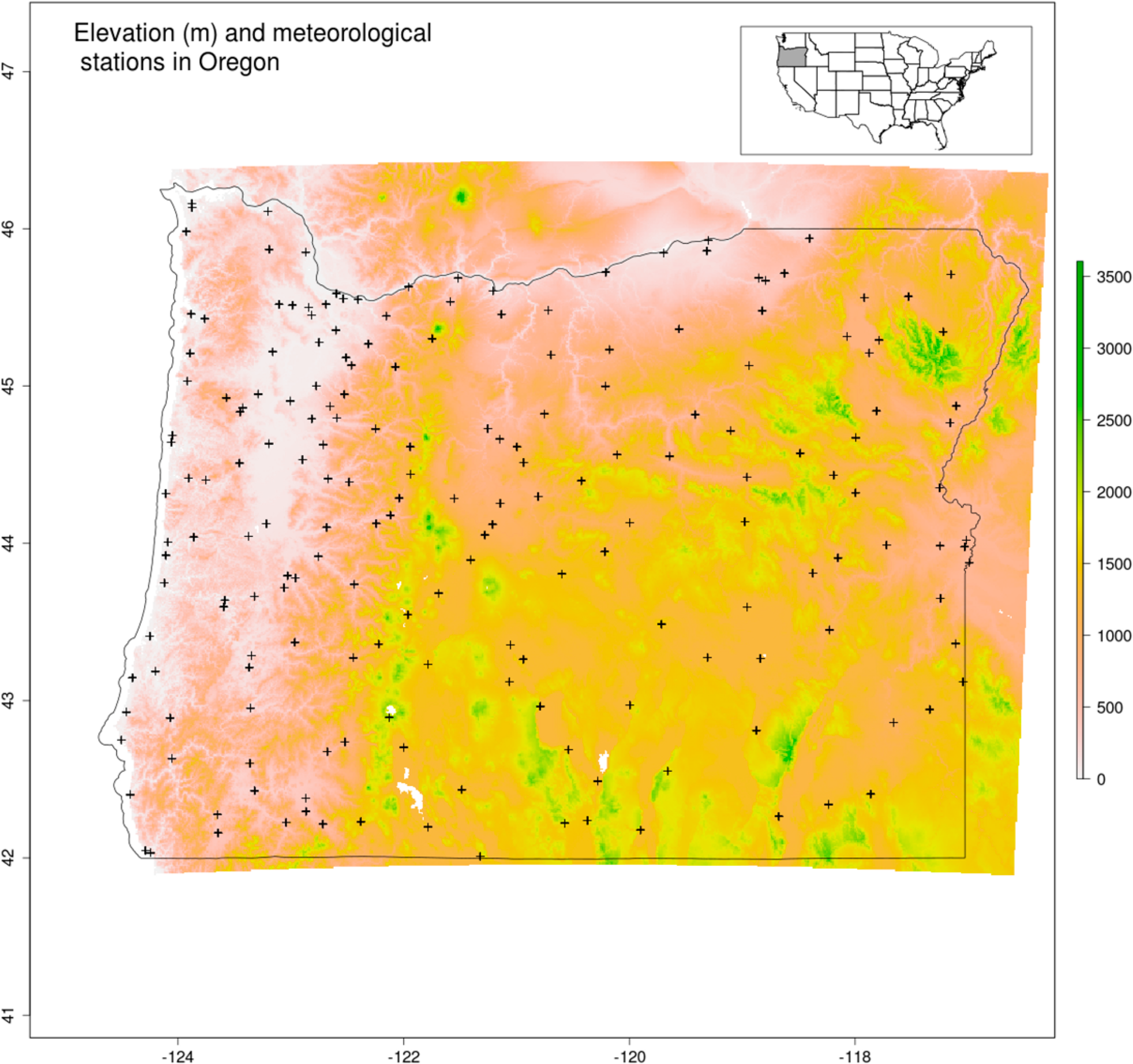
The study region consists of the state of Oregon, USA, and includes 357,000 km2 of land with a complex assemblage of environmental and climatic conditions (Figure 1). Climate and weather are heavily influenced by the Coastal and Cascade mountain ranges, which run parallel to the coast of the Pacific Ocean. More than 50% of the land lies above 1000 m including some high peaks such as Mount Hood (about 3400 m). In the West, a narrow coastal plain stretches from South to North. Inland, to the East and South East lies a large dry basin with arid climate that prolongs the North American Great Basin. The state is also covered by frequent cloud cover which renders the use of remotely sensed data, in particular daily LST a very challenging process (Section 2.3). Oregon’s landscape is dominated by forest, grass and shrubs. Forest cover is the most widespread and often found in high elevation areas. Grass and shrublands are found in the inland basin area in dry environment. Agriculture is concentrated mainly in two valleys; in the Columbia valley in the North near the border with the Washington state and inland in the Willamette valley. The complexity of physical geography and climate on the one hand, along with a relatively good record of historical climate data on the other, makes the region an ideal test case for the model fitting challenges we undertake here.
2.2. Data and Processing
For temperature interpolation, we used ground meteorological stations from the Global Historical Climatology Network assembled by the National Oceanic and Atmospheric Administration (GHCND, [51]). The GHCND database covers the 1763–2013 time period and contains meteorological measurements on minimum and maximum temperature as well as other variables such as precipitation. GHCND contains over 80,000 stations in 180 countries and has undergone a strict quality process to screen errors and record quality information [51,52].
We evaluated nine different covariates (Table 1) including: elevation, Land Surface Temperature (LST, MOD11A1), Forest Land Cover Type, distance to coast, aspect (Eastness and Northness, see below) and canopy height. Elevation was obtained from the Consultative Group on International Agricultural Research which produced a one kilometer surface from SRTM [53]. From elevation, we derived slope (“s”) and aspect (“a”) variables to create weighted aspect variables for Northness (N_w = sin(s) × cos(a)) and Eastness (E_w = sin(s) × sin(a)) [54]. Distance to ocean was generated from the Global Distance from the coast product [55] resampled from 0.01 degree to 1-km resolution (using Nearest Neighbor) to test the maritime effect in Oregon. We also included a canopy height (CANHEIGHT) variable derived from Geoscience Laser Altimeter System on Icesat [56]. The percent forest cover was calculated from the Consensus Land Cover product, which provides prevalence estimations of 12 land cover types at 1-km resolution [57,58]. We used Land Surface Temperature (LST) MOD11A1 product [59] and downloaded tiles h08v04 and h09v04 for the 2001–2010 time period from NASA [60]). LST covariate was used as a long term average climatology to deal with cloud cover, missing values and low quality pixels. Because of its complexity, the processing of LST is described in more detail in the next Section 2.3. All raster datasets of covariates were spatially subset to match the study area and reprojected to the Lambert Conformal Oregon State projection (EPSG 2046).
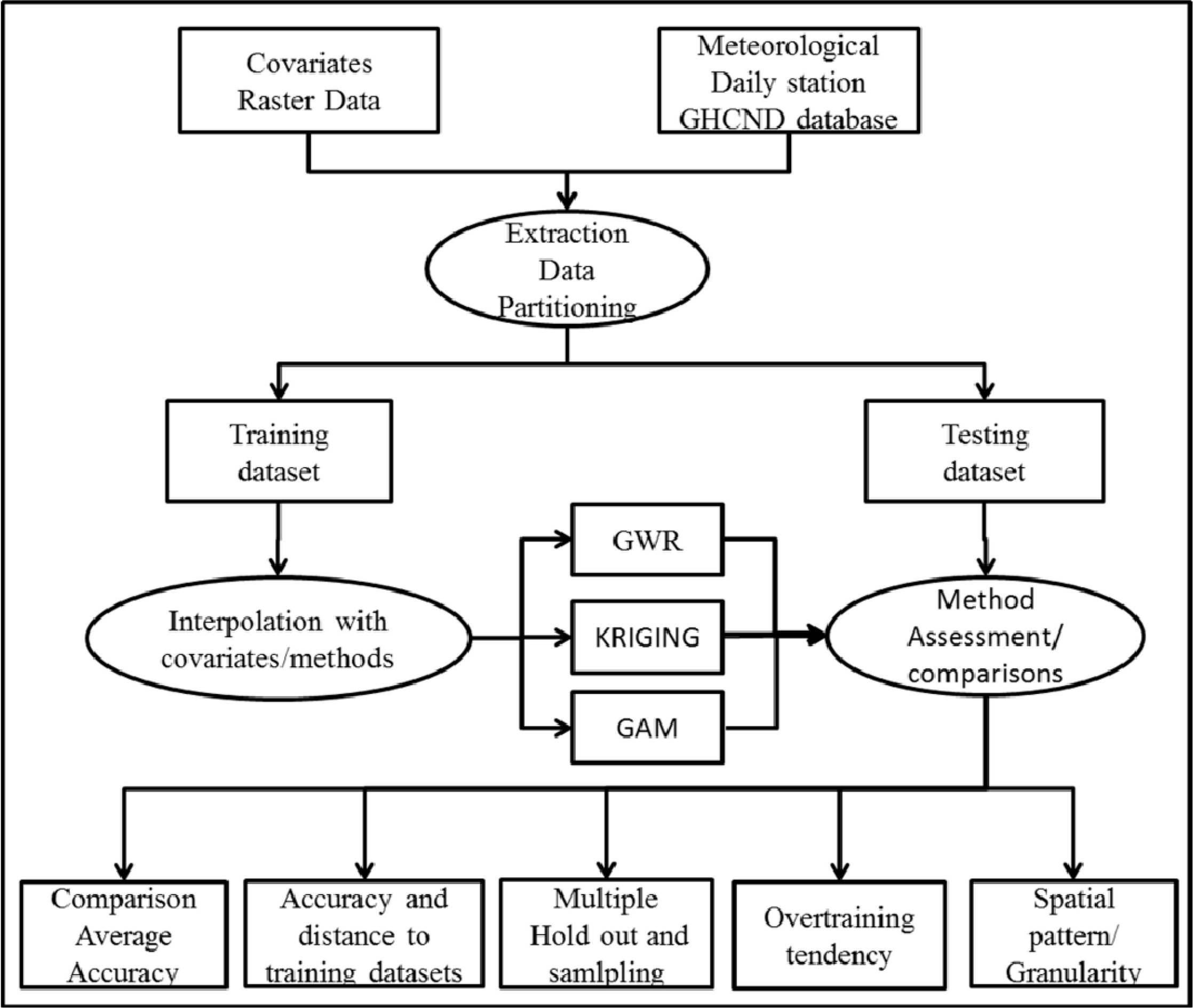
The analysis was conducted in four stages (Figure 2). First, for each GHCND station daily maximum temperatures during 2010 corresponding covariate values were obtained based on the geographic location of the station. Temperature measurements were screened for quality using the GHCND quality flags. The number of stations with high quality data ranged between 134 and 159 with an average of 149 per day. Second, meteorological stations were divided randomly into training and validation/testing datasets using a holdout proportion of 30%. The third stage consisted in fitting the set of interpolation models using the training datasets and predicting daily maximum air temperature for every 1 km pixel in the study area. The process of predictions, models selection and interpolation methods are described in Sections 2.4 and 2.5. In the fourth stage, we assessed results using validation metrics on the withheld data and performed additional analyses (multiple holdouts) to evaluate the predictive performance of the set of models and covariates.
2.3. Production of LST Covariate Surfaces
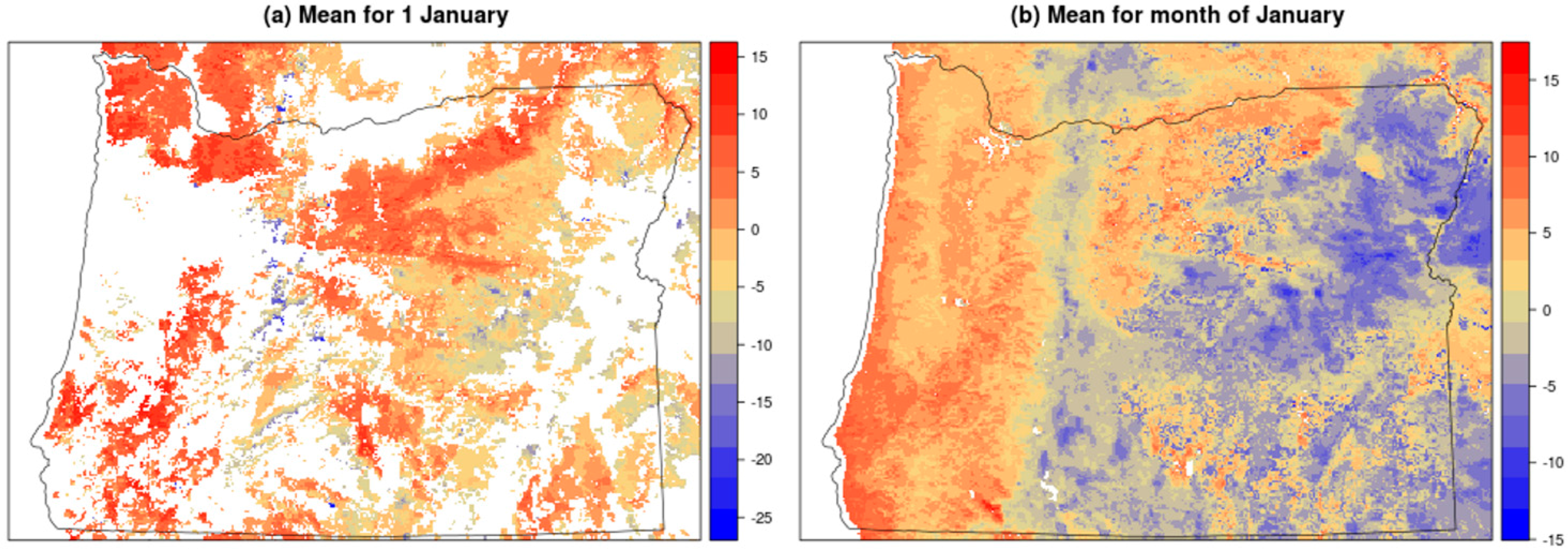
Land Surface Temperature MOD11A1 product required additional processing to prepare covariate surfaces for interpolation. We downloaded and mosaicked the daily images for tiles 09v04 and h08v04 for the 2001–2010 time period. While MODIS collects daily observations at every 1 km location, many measurements may be missing due to the presence of clouds or may need to be screened out due to the low quality values. This was the case for the Oregon study area where the large number of missing daily values prevented the use of daily LST measurements directly in the interpolation process. Given that our goal is to leverage the fine grained content of LST, we dealt with gaps in the LST surfaces by temporally averaging LST values across the time series. Thus, after screening daily values using MODIS quality flags to remove cloud-covered and low quality pixels, we produced long term averages called “climatologies” using observations available over the 2001–2010 time period. We computed daily climatologies for 366 days of the calendar year but found that despite the averaging large spans of Oregon still did not contain any measurements (Figure 3). For instance, for 1 January, 51.3% of the observations in the study area have missing values. We therefore generated 12 monthly long term climatologies by averaging each month over the 2001–2010 time period (after screening for quality). The use of the monthly climatologies reduces the number of missing values and maximizes the number of available observations to capture the LST spatial structure for interpolation.
2.4. Covariate Models and Improvements over Baselines
To evaluate each covariate’s contribution, we used two baseline models that include (1) geographic coordinates only (latitude and longitude); (2) geographic coordinates (latitude, longitude) and elevation. The first baseline is commonly used in the climate literature either in the form of IDW or Universal Kriging while the second baseline includes the well documented lapse rate relationship. For both baselines, we compared the improvement in predictive accuracy by adding each potential covariate to the baseline model (Table 2). We also explored a specified number of interactions of covariates that are hypothesized to be important. For example, LST is known to have different biases depending on land cover type [39] so we explored the improvement in predictive accuracy achieved by adding the main and interaction effects of LST with the percent forest cover (LST*Forest) and canopy height covariates. Each covariate (in combination with the baseline model) was evaluated for the 365 days in 2010.
2.5. Interpolation Methods
Using the optimal model with the set of covariates identified by the methods in Section 2.4, we compared three different interpolation methods: GAM/spline regression, Kriging and geographically weighted regression. GAM provides a statistical framework to bring together and extend many methods found in the literature. For instance, the ANUSPLIN algorithm used in New, Lister, Hulme and Makin [18] and Hijmans, Cameron, Parra, Jonesand Jarvis [22] fits a spline regression [10,11] that essentially falls under the umbrella of GAM [61]. GAMs are regression-based models that use splines to provide more flexibility in the representation of relationships. Splines are piecewise functions built from different bases functions that join at knots. Important parameters to consider when fitting GAM models include the choice of type of bases and knots [62]. Common bases include cubic regression and thin plate spline. After initial exploration of bases and knots, we used the thin plate spline basis with automated selection of knots. Since our goal is to develop and assess methods that can be scaled up easily, we aimed at reducing human inputs in the fitting of the daily models. Thus, we used automated knots selection with estimation of smoothing parameters from generalized cross validation (GCV) as implemented by Wood [61] in the R mgcv package. The GCV procedure, used to select knots and smoothing parameters, was carried using only the “training” dataset mentioned above.
Kriging methods such as Ordinary Kriging and Universal Kriging are frequently used to interpolate surface [63–66]. The general idea is to leverage spatial autocorrelation present in the observations to generate new predictions. Kriging methods have a well-developed body of theory that allows for the calculation of uncertainty [67,68]. Developed first in the geostatistics literature, kriging can be mathematically related to regression and spatial autoregression literatures [69–71]. The statistical motivation for kriging is to account for the common situation in which variables at nearby locations are expected to be similar using a kernel function (also known as covariance function or variogram [72]) that models the spatial relationship among neighboring values. In Kriging, variability is partitioned into a global component and a local component. The global component is modeled through a trend surface that may include covariates in which case the method is often referred to as Universal Kriging [64] or regression Kriging [73]. In this study, we experimented with Universal Kriging with geographic and environmental covariates. Since the choice of the variogram often requires extensive user inputs and since our goal is to assess methods with few human inputs for later scaling up, we used automatic fitting of variograms based on the weighted least square method pioneered by Cressie [74,75]. This method, recently used by Hiemstra et al. [76], provides the flexibility of fitting variograms at a daily time step in an automated fashion by fitting sequentially a series of variogram models and using the SSER (sum of squared errors) criteria to choose the appropriate parameters and models for operational applications. We used the kriging implementation from gstat and automap packages in R [76,77]. There are four common variogram models tested for automatic fitting: “Spherical”, “Exponential”, “Gaussian” and “Stein” [78]. The “Stein” model is a Matern variogram model that uses the parameterization from Stein et al. 1999 [79].
Geographically Weighted Regression performs a multiple linear regression but allows smooth, spatially varying coefficients [80]. GWR is implemented through a local regression using covariates and weighting of observation by a kernel function. This allows GWR to estimate the relationship of the response and the covariates locally rather than globally and is thereby capable of accounting for heterogeneity within a region. As an example, GWR can estimate a spatially varying lapse rate. GWR first estimates a “neighborhood range”, typically using generalized cross-validation (GCV), and second, fits the kernel model function [80]. GWR is very similar in approach to the methods that Daly and colleagues used in the PRISM product [37,81] where regression coefficients vary spatially. In this study, we used the Gaussian exponential model and the range was automatically determined for every daily prediction using GCV of the training set (again with the aim of developing and assessing methods with minimum human inputs for scaling up purposes). Predictions were performed using the spgwr package available in R [82].
2.6. Assessment and Comparison of Models
To assess models, we calculated five accuracy metrics Mean Absolute Error (MAE), Root Mean Square Error (RMSE), Mean Error (ME) and Pearson’s Correlation Coefficient (r)—by comparing the holdout station observations to their corresponding predicted values in the predicted surface. The MAE, RMSE and R were used to evaluate the average error while the ME metrics was used to evaluate the average bias. Although the properties of these metrics are fairly well understood [83], it is not obvious what the best inferential framework to use in evaluating interpolations. The challenge with evaluating interpolations is that the true values are generally unknown at most locations. Machine learning and statistical methods address this problem using the cross-validation approach where a fixed fraction (e.g., 70%) of the data is used for training the model and then the remainder (i.e., 30%) is used to test or validate the prediction accuracy [49,50]. To our knowledge, there are no well-developed best-practices for using a hold-out approach in spatio-temporal autocorrelated data such as weather station data. Here we examine:
The effect of different proportions of holdout (10%, 20%, 30%, 40%, 50%, 60%, 70%) on prediction accuracy and interpolation methods.
Which models are the best at predicting hold-out stations farthest from the training stations (i.e., if/how predictive accuracy decays similarly with distance from training stations for all models).
The “over-training” or overfitting tendency of interpolation methods, which can be quantified by the sensitivity of the validation metrics to the samples used for fitting the models. Overtraining occurs when fit based on the training dataset is very good but there is low accuracy in the testing dataset resulting in large differences between training and test accuracies. This effectively means that the model lacks generality or that noise in the training dataset has been fitted into the model. We examine this phenomenon across the full year and with different holdout and random samples to account for the effect of variation in training and testing datasets.
Whether the scales of spatial variability were realistic. Because detailed ground-station data at very fine grain-sizes were unavailable, we were forced to use indirect and less objective methods. First we examined the granularity of prediction by visual inspection and image differencing. Second, we calculated a plot of spatial lag autocorrelation to illustrate the inflation of spatial autocorrelation in models lacking granularity.
3. Results and Discussion
3.1. Covariate Improvements over Baselines
We summarized results for the two baselines in Table 3 using the GAM method. Each value shows the improvement relative to the baseline when a specific covariate is included. Baseline 1, which includes latitude and longitude covariates, has the following (mean ± standard deviation) accuracy values: MAE = 2.226 ± 0.496, RMSE = 2.919 ± 0.625, ME = −0.018 ± 0.535 and r = 0.6 ± 0.210 (Table 3). For the first baseline, we find substantial improvement only by adding elevation (decreases of 0.437 and 0.296 in RMSE and MAE respectively) and LST (decreases of 0.117 and 0.057 in RMSE and MAE, respectively). Adding the interactions between LST and canopy height and between LST and percent forest cover also slightly improve the baseline 1 model, suggesting that these covariates may be important or useful.
Baseline 2 which includes latitude, longitude and elevation, has an MAE of 1.930 ± 0.519, RMSE of 2.482 ± 0.654, ME of 0.015 ± 0.467 and Pearson r of 0.738 ± 0.148 (Table 3). For the second baseline, results are less differentiated and most models exhibit accuracy values similar to the baseline model. The incorporation of covariates does not improve the accuracy with the exception of DISTOC, for which we see a very slight decrease of MAE and RMSE (Table 3). All other models display increases in MAE ranging between 0.019 (for model including LST) and 0.065 (for model including LST and CANHEIGHT). Based on accuracy metrics, the three top models are the DISTOC and baseline 1 model followed by the LST model. We performed Kruskal-Wallis tests and found that only elevation improved baseline 1 (lat*lon) statistically significantly (at p < 0.05), but that none of the covariates significantly improved baseline 2 models. In summary, adding elevation greatly improved the accuracy but no other covariate greatly improved the model, although DISTOC showed some potential. LST and LST interacting with canopy height improved the model without elevation (baseline 1 models) but not the model with elevation (baseline 2 models). Nonetheless, because LST varies at a finer spatial grain than Latitude, Longitude and Elevation and because there is potential that ground weather stations are a biased sample of canopy height, both covariates might merit additional future evaluation, especially if data on fine-grained temperature sensor networks become available.
3.2. Interpolation Methods
Using the top set of covariates (latitude, longitude and elevation) identified in the previous step, we compared the interpolation methods using averages for the MAE, RMSE, ME and r accuracy metrics (Table 4). We find that the GAM method has the best (smallest) RMSE and MAE, the best (largest) r, and the second best (smallest) mean bias as measured by ME. GAM also has the smallest standard deviation across the 365 days of 2010 for RMSE, MAE and ME metrics (Table 4). Thus, in nearly all metrics, GAM outperforms GWR and Kriging methods although the magnitude of differences is small. This is confirmed by the Kruskal-Wallis test which reports that differences among models are not significant (p > 0.1). This suggests that we must move beyond the comparison of aggregated average metrics, even on held out data, to understand differences in performance among interpolation methods.
3.3. Assessment Methods
3.3.1. Accuracy in Terms of Distance to Closest Training Station
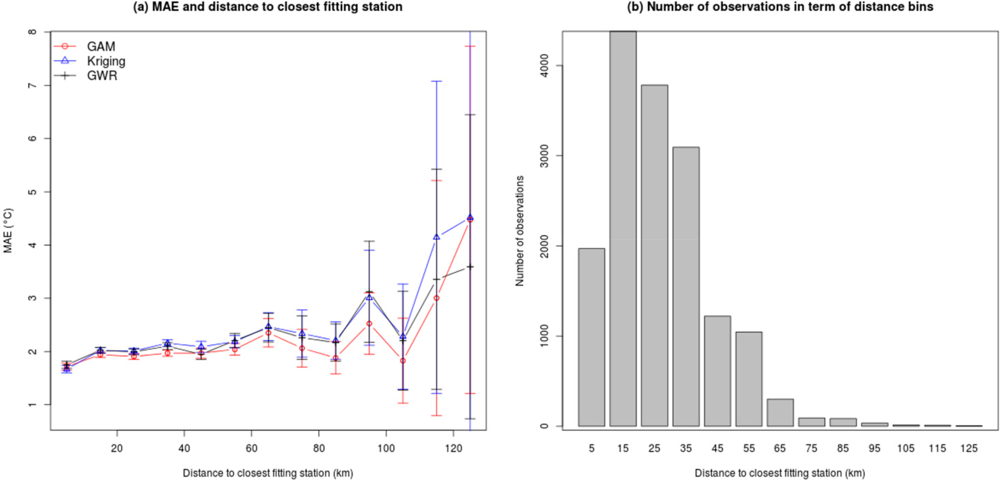
We expect better prediction accuracy in cells that are closer to fitting stations than further away. In order to test this concept, we calculated the variation in MAE in terms of the distance to the closest training station for all three interpolation methods using the optimal model identified earlier, i.e., the model including latitude, longitude and elevation (baseline model 2) with 30% holdout. Figure 4 indicates that there is a modest increase in MAE with distance but it becomes erratic at larger distances due to the high variability for all methods. Average MAE for GAM is the lowest in the first bin, centered at 5 km, with a value of 1.749 °C and increases roughly linearly to reach 2.449 °C at 65 km. Errors in bins beyond 65 km are noisy but display a general positive trend resulting in a MAE of 3.591 °C at 125 km for GAM. Errors bars (95% confidence interval) indicate that variability is high for high distances rendering any strong statement difficult. Uncertainty at farthest distances is due to the low number of observations as illustrated by the histogram of frequency by distance bin.
Figure 4 also reveals that the GAM method has, on average, a lower MAE per distance bins. Thus, results suggest that the GAM method outperforms GWR and Kriging at all distances from the station and is the best at including information from nearby while balancing overall testing accuracy.
3.3.2. Multiple Hold Out Proportions
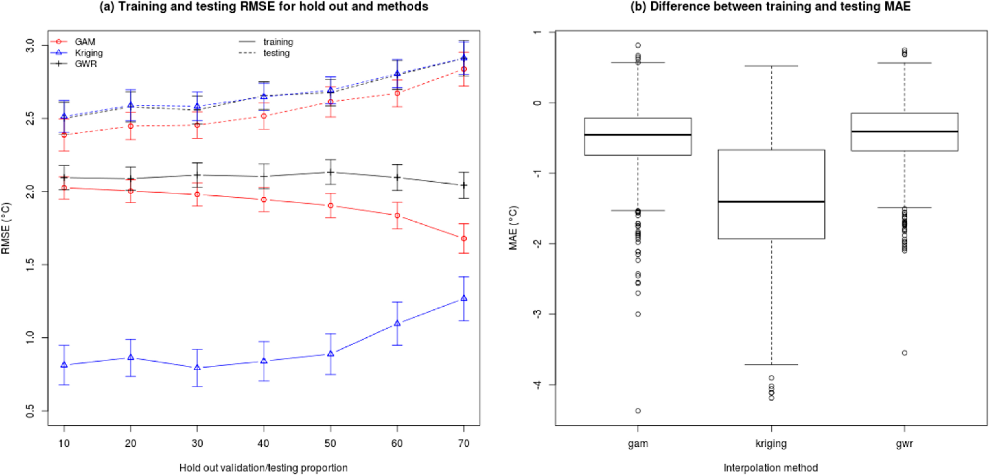
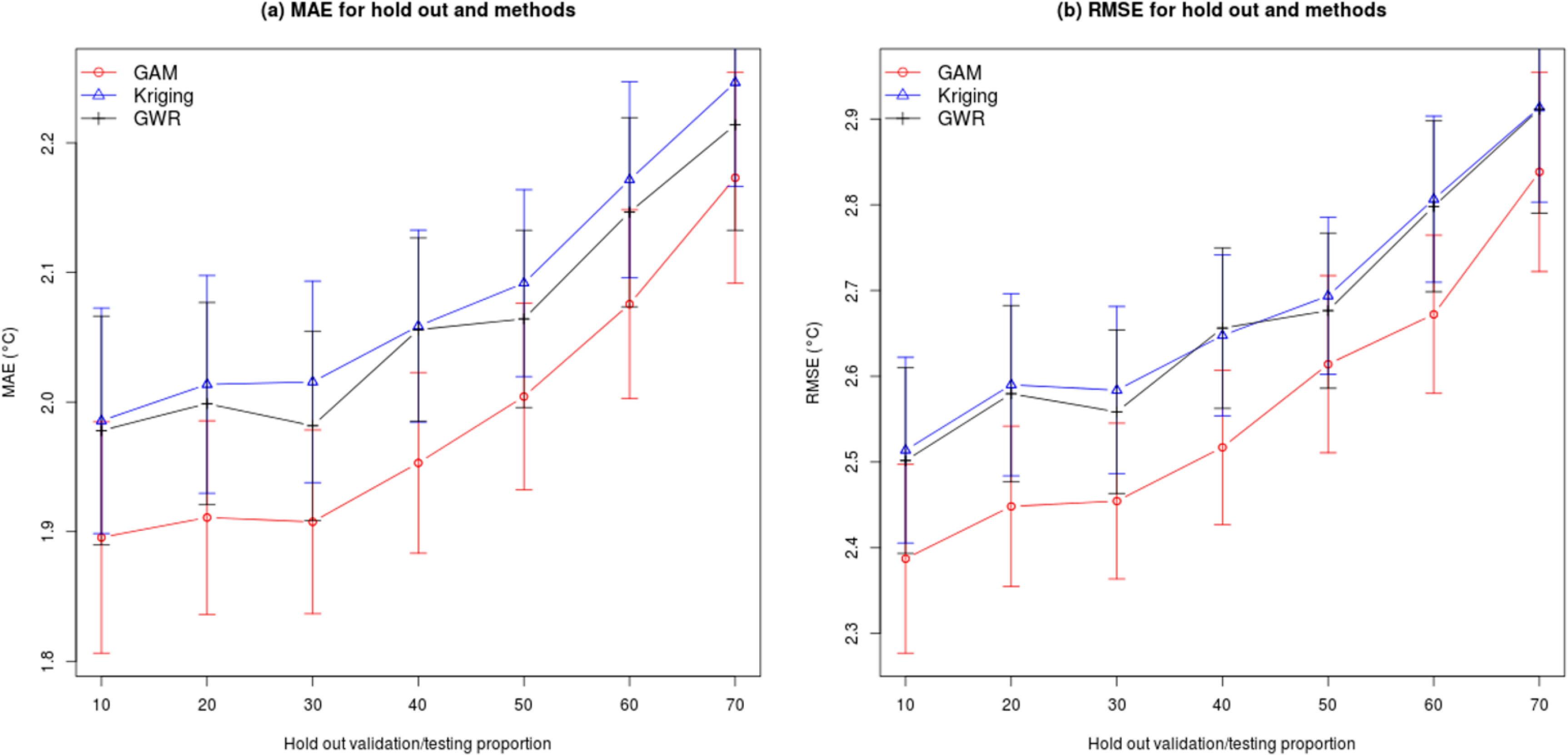
Previous studies also suggest that the choice of the proportion of hold out and random selection affect the accuracy of predictions. To take this issue into account, we assessed models by varying the holdout proportion from 10% to 70% with random samples for each proportion and interpolation method. Due to the high computational load, we used every other day or 183 dates spread evenly over a full year rather than 365 dates. For each hold out proportion, we have 183 outputs which sum up to 1281 predictions in total per interpolation method. We plotted RMSE and MAE for each hold out proportion and interpolation method (Figure 5) to summarize results. As expected, RMSE and MAE increase (i.e., prediction accuracy decreases) when more stations are excluded from the training dataset (i.e., held out) for all three methods (Figure 5). The 95% confidence intervals are about 0.1 °C and 0.2 °C for MAE and RMSE, respectively, and remain constant for all proportions of hold out with the exception of a slight increase at 70%. Results show that GAM method (in red) has on average a lower MAE and RMSE for all proportions of hold out when compared to Kriging (in blue) and GWR (in black) methods. These results suggest that the GAM method is the most resistant to variation in hold-out proportion.
3.3.3. Over-Training: Overfitting Sensitivity to Samples Used for Training
Generality of models is an important property that is sought in predictive models. This means that the relationships that are modeled from the data must meet the sometimes conflicting objectives of fitting the training data but also predicting well to other locations or times [49]. Similarly, training datasets must be large enough to represent the existing pattern while the validation dataset must be large enough to allow correct estimation of accuracy. In the machine learning and statistical fields, the training information is typically split multiple times with various hold out proportions (k fold cross validation) to tackle over fitting issues [49,50]. If the split datasets diverge greatly in accuracy, then it is inferred that the model is not general enough and suffers from a tendency or sensitivity to overfit (“overtrain”) the training information. In the machine learning literature, this is often used to choose the optimal model complexity [84].
Building on previous results, we used testing and training datasets to identify a sensitivity to the size and selection of samples for training. We measure this sensitivity to overfit in predictions using variation in holdout proportion and random samples (Figure 6a) for 183 dates (every other day in a year). To visualize divergences, we plotted average RMSE for training (solid line) and testing (dashed line) datasets for each hold out proportion and methods (Figure 6a). The difference in RMSE between training and testing datasets is a measure of overfitting, with larger differences indicating more serious overfitting. Results reveal that the difference in RMSE is the largest for Kriging compared to GWR and GAM methods (Figure 6a). We also find that Kriging has larger differences in MAE with a median of −1.5 °C compared to −0.3 °C for GAM and GWR (Figure 6b). The spread of value is also smaller in magnitude for GAM and GWR methods which show quartiles of 0.2 °C compared to 0.5 °C for Kriging (Figure 6b). Thus, results indicate that GAM and GWR are less sensitive to overtraining/overfitting and that GAM has the lowest prediction errors. We also find that Kriging has the largest tendency/sensitivity to overtrain and is more strongly affected by the removal of observations.
3.3.4. Differences in Spatial Pattern, Variation and Granularity
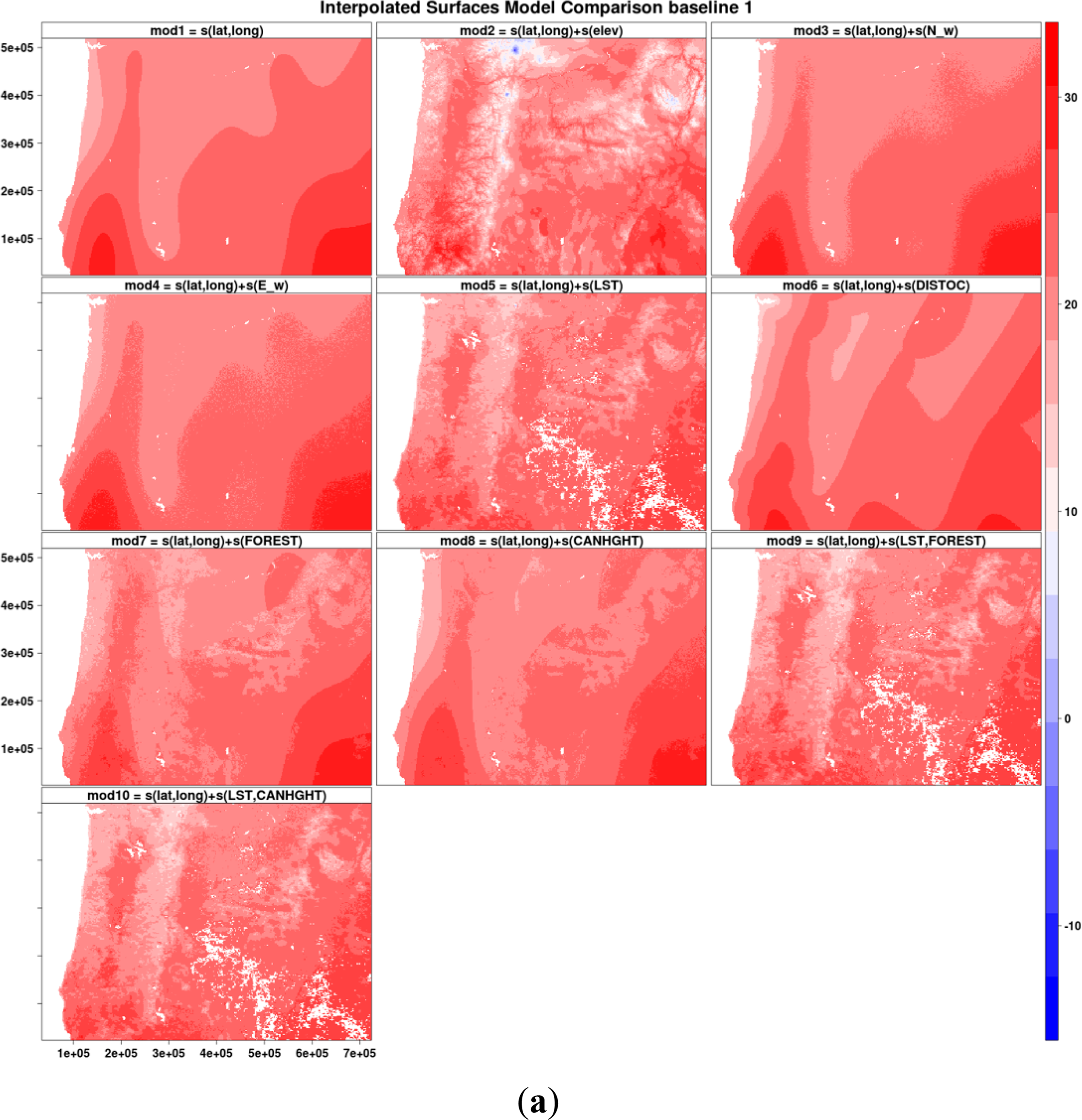
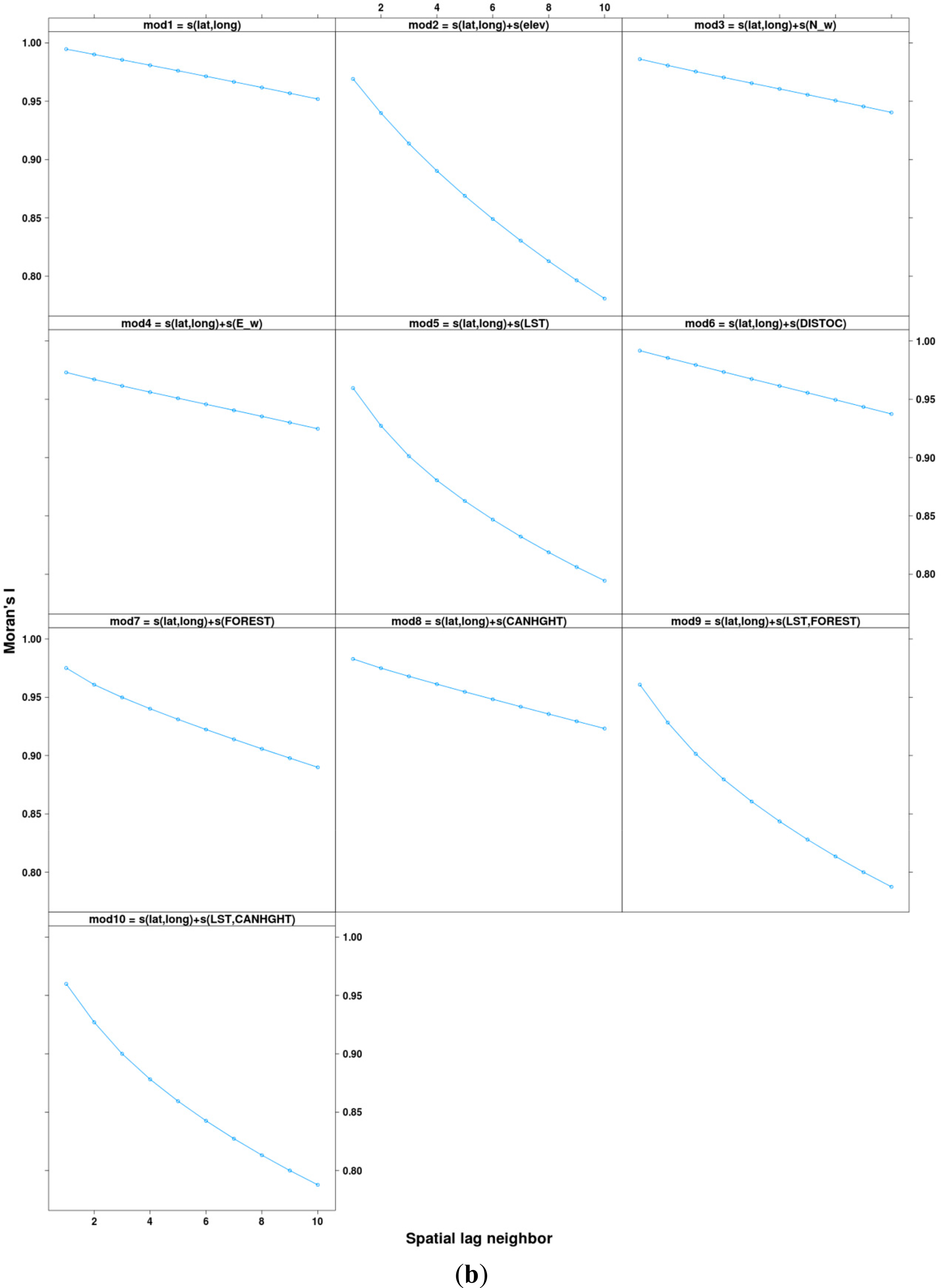
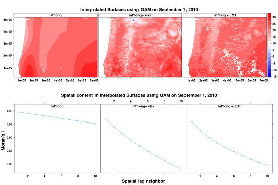
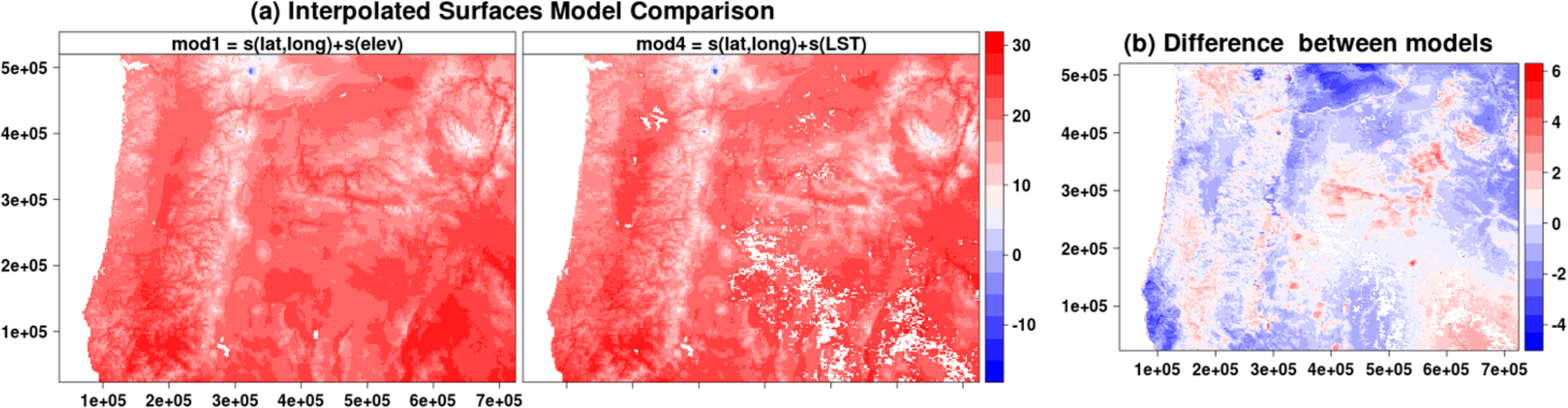
We examined spatial prediction patterns for baseline 1 models (Figure 7a) and found that models without LST or elevation have very smooth interpolated surfaces with little spatial variability. The Moran’s I-index spatial correlograms for distances ranging from 1 to 10 pixels (using Queen’s neighborhood rule) also show that models without elevation or LST have inflated autocorrelation manifested by the slower decreasing autocorrelation trends (Figure 7b).While accuracy metrics alone do not suggest superiority of LST over elevation both LST and elevation provide spatial structure and fine-grain variation that is lacking in other covariates (Figure 6). Additionally, difference in predicted maximum temperature for 1 September 2010 between baseline 2 (lat, lon and elevation) and baseline 2 + LST (lat, lon, elev and LST) models reveals that LST adds fine-grained spatial variability not captured by the elevation layer (Figure 8). Much of the difference in spatial structure relates to land cover effects as visible from the agricultural areas in the Willamette Valley and in the Northern part of the region near the border with the state of Washington State. Unfortunately, at the present time, adequate ground station data at fine grain-sizes do not exist to allow more objective evaluation of the accuracy of this fine-grained variability.
3.4. Discussion
Results from average accuracy metrics over a full year (Section 2.3) suggest that although differences are small, GAM consistently outperforms GWR and Kriging methods and that there is little improvement in accuracy when covariates are added to a model already containing latitude, longitude and elevation. Since these results are obtained by coarsely summarizing the accuracy metrics across 365 days, they may hide important temporal patterns. Thus, we examine and discuss in more details (1) variograms’ model and parameters across the year; (2) residual maps; (3) the monthly temporal variability in accuracy; (4) the contributions of covariates daily and monthly over 2010.
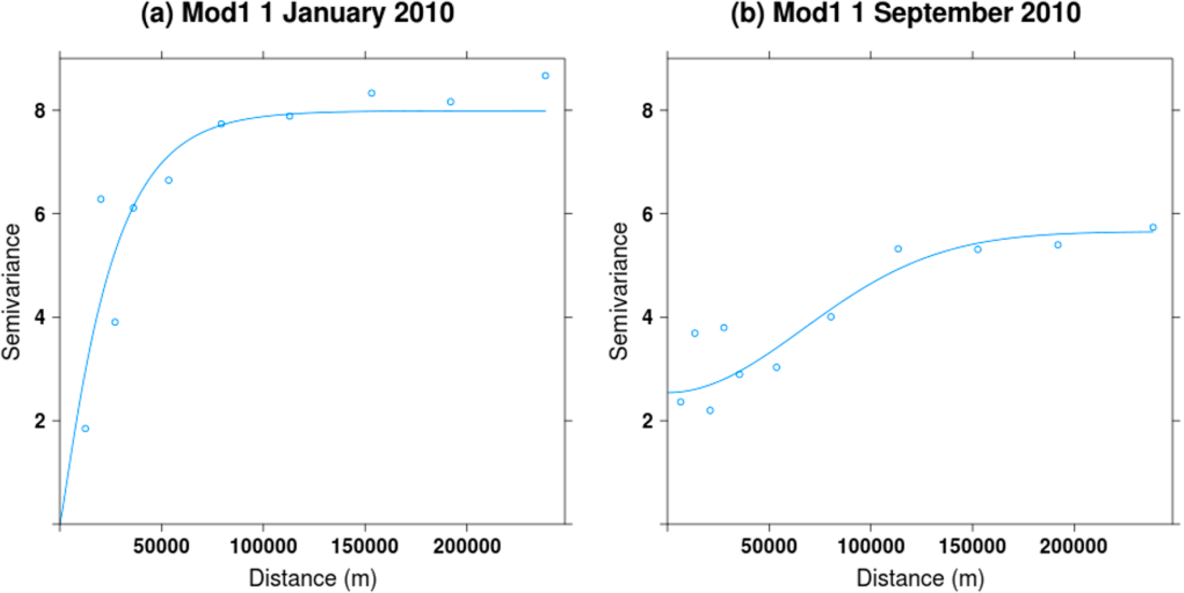
3.4.1. Temporal Variation in Fitted Variograms
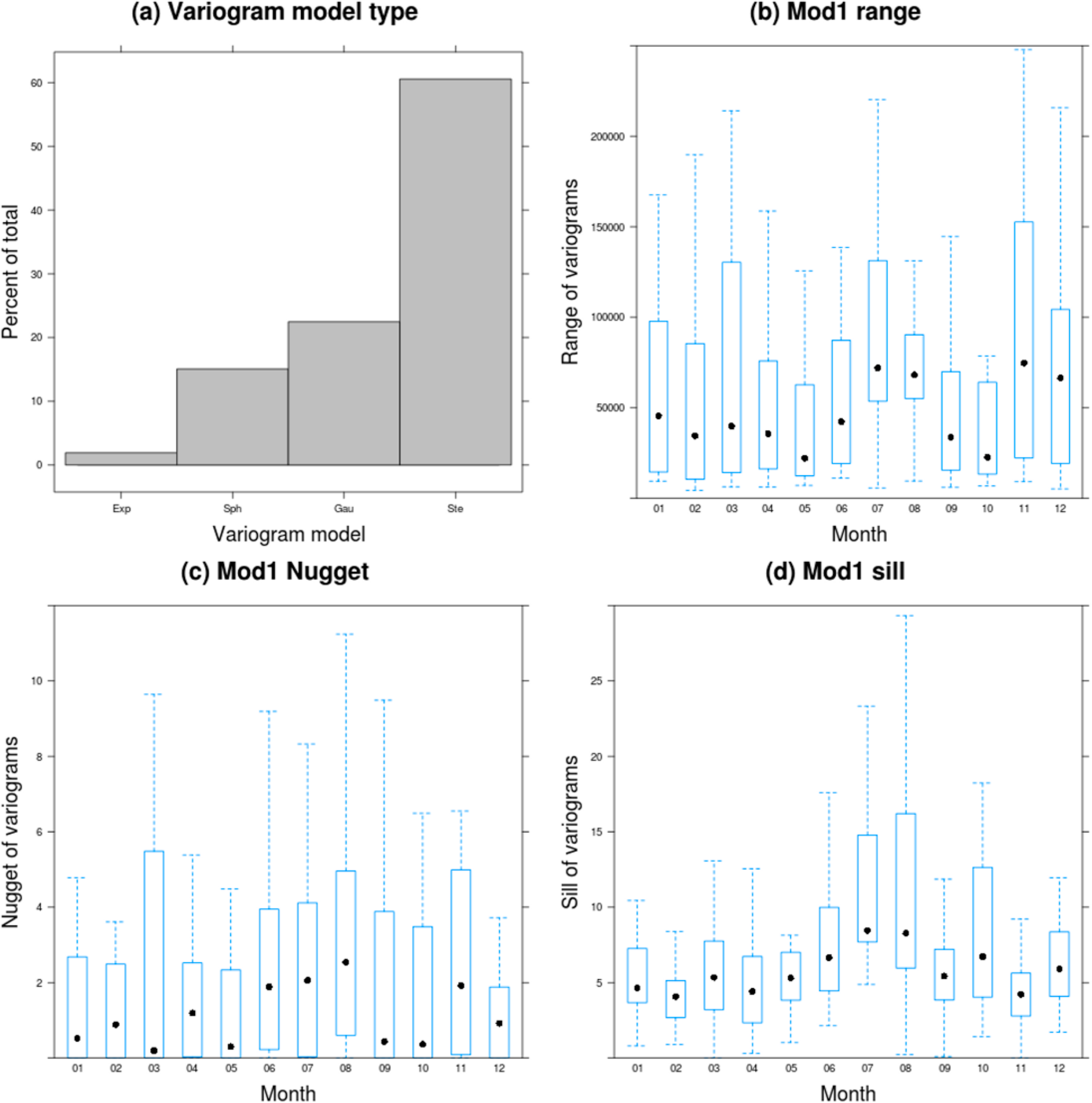
It is not possible to show all variograms for the year 2010 since they are fitted at the daily timescale. We therefore provide a visualization for two dates—1 January and 1 September 2010—(Figure 9) as well as a summary of fitting parameters (Figure 10). Of the four variograms models tested sequentially, we found that the Stein (Matern) variogram [79] was the most commonly selected across the year (60%) (Figure 10). We also found that there is important seasonal variation in the shape of the fitted variograms (Figure 10). In particular, we found that sills and nuggets are greater for June, July and August. The large variation in fitting across the year suggests that it is useful to allow for variograms to vary intra-annually.
3.4.2. Residuals Maps
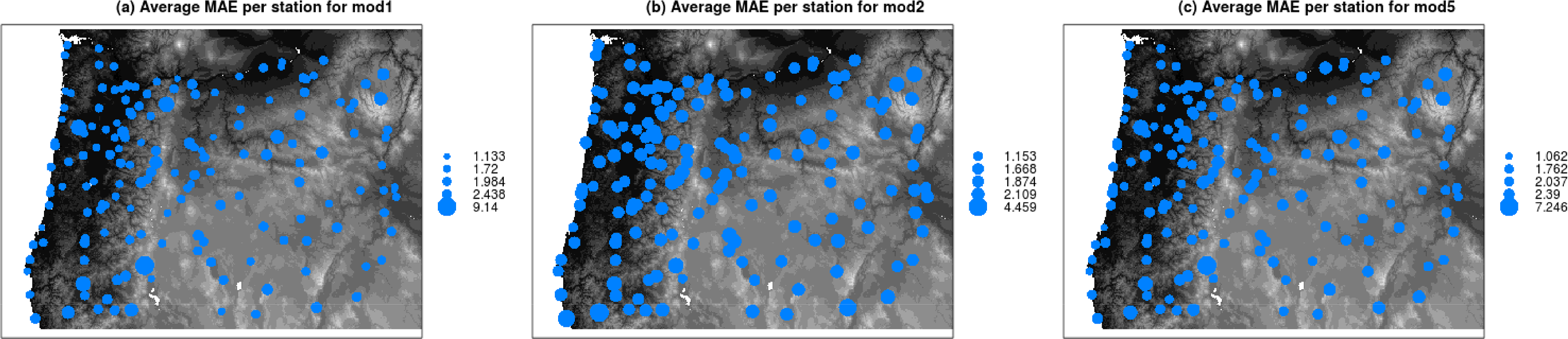
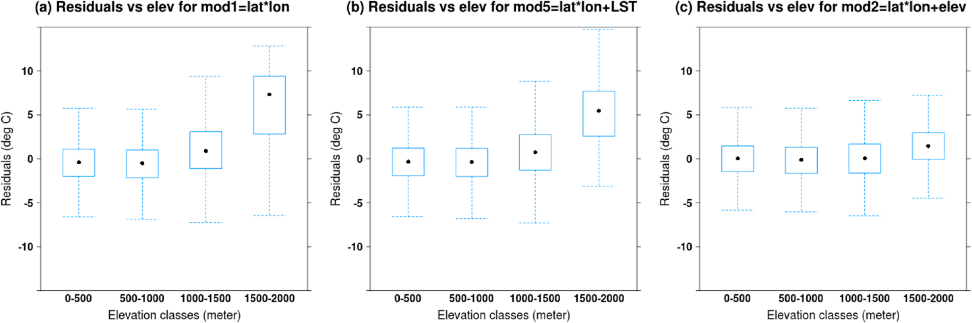
We examined residuals maps for several daily predictions to uncover spatial patterns in errors without success (e.g., Figure 11 for 1 September 2010). In an attempt to gain more insight, we summarized errors at daily stations using average MAE for baseline 1 and baseline 2 and the model including LST (Figures 12 and 13). Figures 12 and 13 suggest that stations with larger errors are typically found at higher elevation, but the inclusion of LST and elevation reduces the MAE (Figure 13). Elevation decreases more RMSE in higher areas than LST. This also confirms that elevation and LST do not contain the same information.
3.4.3. Temporal Variation in Accuracy
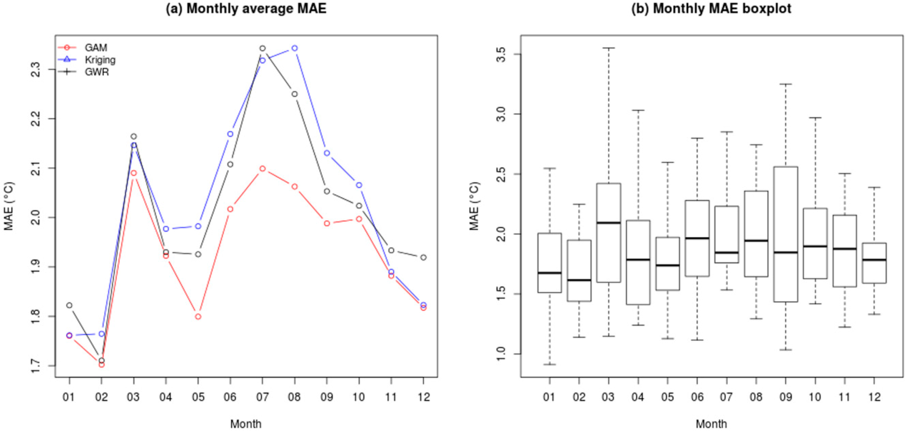
To explore temporal patterns, we summarize accuracy metrics by month for all three interpolation methods. We find that GAM (in red) has lower RMSE than Kriging (in blue) and GWR (in black) over the 12 monthly averages (Figure 14a) but the magnitudes of differences are small. Contrast among interpolation methods is the most important in July and August with differences in mean RMSE reaching 0.3 °C while in winter, methods perform similarly. MAEs for all three methods are larger during summer months with differences between max and min of about 0.5 °C. We also note the presence of a peak at 2.1 C in March. Boxplots reveal that variability is important month by month with quartiles mostly in the 0.3 C–0.5 °C range (Figure 14b). The summary table, which includes standard deviations (Table 5), confirms that models exhibit the largest variances during summer months (July, August, and September) with the exception of March/April. The highest standard deviation occurs in August for Kriging (0.924 °C) and for GWR (0.846 °C) and; in April for GAM (0.850 °C). While the mean RMSE varies greatly over the 12 months, Kruskal-Wallis test indicates that monthly differences are not significant with the exception of summer months for GWR and Kriging methods. Finally, we note that the GAM method has the lowest seasonal signal in the errors suggesting that it outperforms other interpolation methods.
3.4.4. Assessing the Contribution of Covariates and LST
With the advent of Earth observation datasets, much hope has been put in remotely sensed datasets to improve estimation of air temperature and precipitation [46]. Other researchers have used LST to predict air temperature but few previous studies [42] have compared the contribution of LST in relation to other existing covariates for daily predictions with holdout. Our research thus provides a more general assessment of LST products with both evaluation of covariates and interpolation methods. Surprisingly, we found that, when considering patterns over the whole year, LST contributes little to the accuracy as measured by validation metrics when elevation was already included but that LST and elevation do both include spatial fine-grained content that is not found in other covariates. In order to better understand this issue, we examine information from the training dataset and identify the number of times LST and other covariates are flagged as significant over 365 days for p-value thresholds of 1%, 5% and 10%. For baseline 1 models, we find that elevation is flagged the most frequently (348, 356 and 359 times at 1%, 5% and 10% levels) followed by the terms “lat*long”, LST and DISTOC (Table 6). LST is flagged significant 85, 151, 192 times at threshold levels 1%, 5% and 10% for baseline 2 compared to 297, 340, 350 times for baseline 1 models (which do not include elevation in the baseline). All other covariates are less frequently flagged as significant with the exception of DISTOC. We note that MAE calculated on training (calibration) data, MAE calculated on testing (validation) data and GAM AIC show improvements when additional covariates are added in succession to baseline 1 models. This is in contrast to baseline 2 models for which only the MAE on training data shows slight improvements while the validation metric MAE_v show no improvement or even an increase in error (Table 6).
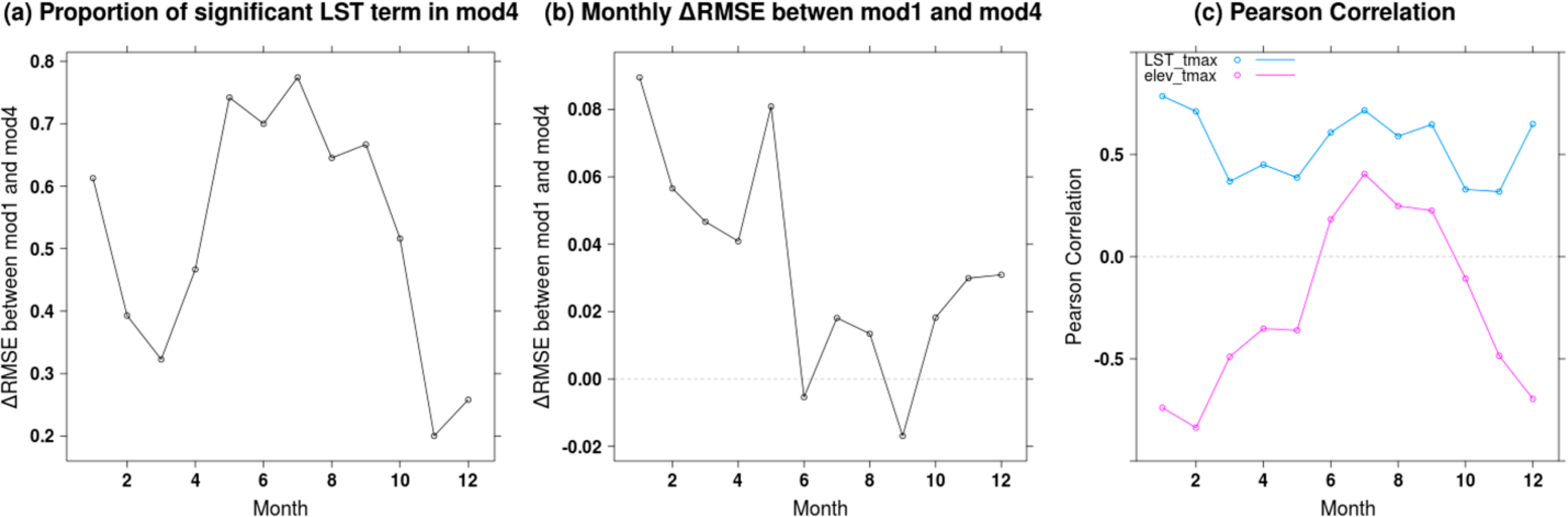
Previous results (Table 6) confirm that LST is an important variable but due to its co-variation with elevation its impact is minor in baseline models that include elevation. We computed the correlations among all raster covariates and found that LST monthly averages and the elevation layer have strong and negative correlation values in winter (with a peak at −0.8) and low positive correlation values in summer (Table 7). By considering significance and correlation monthly, we also found that LST is flagged as significant more often during the summer than during spring and fall (Figure 15). Similarly, during summer, the correlation between LST and air temperature is stronger than the correlation between elevation and air temperature and differences in RMSE between model 1 (lat + lon + elev) and model 4 (lat + lon + elev + LST) are either close to zero or negative. These patterns suggest that there may be a potential for LST to be used during the summer months to improve models. This hypothesis should be explored further across multiple years and in other study areas in future research. Table 7 also highlights that there are large intercorrelations among covariates. For instance, LST shows strong association with Forest and Canopy Height during summer months (typically r = −0.8) which probably relates to the decreased summer surface temperatures in areas with seasonal vegetation. Distance to coast (DISTOC) and longitude also exhibit a very strong relationship (r = 0.97) due to the longitudinal orientation of the state that runs parallel to the South-North coastline.
Our results differ from Kilibarda et al. 2014 [42] findings of improvements in accuracy by using LST for Tmax but not for Tmin and Tmean predictions. Potential explanation for this divergence may include the aggregation of LST at the monthly time scale, the inclusion of elevation, the use of spatio-temporal kriging as a method as well as the use of leave one out cross-validation instead of 30% hold out. Kilibarda et al. 2014 [42] do not evaluate the fine grained spatial content but report the important visual impact of LST and elevation in the temperature predictions which we measured in a quantitative manner using Moran’s I correlogram in this study. We plan to explore these differences in future research by using long term monthly LST averages in multi-time scale methods (Parmentier et al. In Review [85]) such as Climatology Aided Interpolation (CAI [86]) and by using spatio-temporal kriging methods.
4. Conclusions
In this paper, we provided a unique general assessment of remote-sensing derived covariates including LST and interpolation methods using a wide range of assessment procedures. Besides the inclusion of accuracy metrics, we showed that researcher should visualize and quantity the spatial variation in the predicted surfaces.
In quantitative metric terms, results from baseline 1 (lat*lon) indicate that including elevation and LST covariates improve the baseline model the most with decreases in RMSE of 0.437 °C and 0.233 °C, respectively. Models including distance to coast (DISTOC) showed improvements in accuracy and might display stronger improvements in study areas where the coastline is less collinear. We found that there are very few improvements in accuracy among models when the baseline includes geographic variables (latitude and longitude) and elevation (baseline 2). Using average accuracy metrics over 365 days, we compared GAM, GWR and Kriging using the optimal model identified earlier, i.e., the model including latitude, longitude and elevation (baseline model 2). We found that GAM consistently outperformed both Kriging and GWR methods with an RMSE of 2.48 °C compared to 2.59 °C and 2.61 °C, respectively, but that the differences among models are small in magnitude.
We highlight the need for much more rigorous methodology for comparing interpolation methods. Within this study, we were able to incorporate objective assessments of the effects of more station hold outs and of distance to nearest station (effectively studying effects of station sparsity) and to assess a metric of overfitting. These more rigorous evaluations were key to singling out GAM over kriging and GWR. In particular, findings indicate that GAM has the lowest errors in term of the distance to the closest fitting station except when distances are very large. GAM also shows lower errors in function of proportion of hold out. Furthermore, we found that Kriging has a tendency to overfit the data when compared to GWR and GAM methods as indicated by large differences between training and testing accuracies.
Visualization of predictions show that fine grained variation is lacking and that spatial autocorrelation is inflated in models that do not include LST and/or elevation. This point is not surprising because the median and mean distances to nearest station in the study region are 20 km and 22 km (with a 12.5 km standard deviation and maximum of 72.5 km), while LST and elevation are measured and incorporated into our models at the 1 km grain. Image differencing suggests that LST contains spatial variability (related to land cover) which is not found in elevation. The strong summer correlations with air temperature also suggest that LST might improve accuracy during that season. Taken together, this suggests (but we acknowledge does not prove) that LST could improve predictive accuracy given sufficient station density that is not available in this region. As a novel way of assessing fine grained content, the study also introduced the use of spatial lag correlogram to quantitatively measure spatial content in predicted surface. We hope that this practice will be followed in future accuracy assessments of interpolated surfaces.
More succinctly, our case study indicates that:
- (1)
All the interpolation methods give similar results for average accuracy term over a full year. It is necessary to provide additional procedures to differentiate the methods.
- (2)
GAM is the most resistant to hold out variation, less sensitive to overfitting and has the lowest error in term of distance to the closest stations. Kriging is highly sensitive to overtraining.
- (3)
The most important covariates are elevation, LST and DISTOC with the fine-grain spatial variation contained in elevation and LST covariates. Validation on hold-out stations from existing networks does not show improvements from this fine-grained variability but spatial Moran’I correlograms show important differences in spatial content.
- (4)
Based on annual average accuracy metrics, we found that LST does not improve models when elevation is included with latitude and longitude as covariates. During summer however, LST improved models marginally for two months and displayed stronger correlations with tmax than elevation with tmax. When LST is added to models with latitude and longitude, there is a clear improvement in annual average accuracy.
This study highlights an important data gap; there are now several efforts to produce fine-grained weather and climate interpolations but often insufficient data to accurately assess the fine-grained interpolated surfaces. Going forward, it will be important to implement fine-grained ground-station data collections to allow for robust and objective validation of interpolation methods and fine grained products. In summary, this study shows that using GAM (splines) with latitude, longitude and elevation of covariates would represent current best practices for daily temperature interpolation (in the context of Oregon using current station data). We also found suggestive evidence that LST could be to improve accuracy during summer and contribute to the fine grained content of predicted surfaces but that denser station data (in spatial subregions) are needed to assess this. We are currently working on producing high quality LST filled climatology for global use in interpolation. Although beyond the scope of this paper, multiple time-scale methods (e.g., climate aided interpolation see [86]) and spatio-temporal kriging [84] need to be evaluated for their ability to produce daily fine-grained predicted surfaces. Given the current high demands for fine-grained weather and the likelihood that this demand will only increase, it is vital that more attention is paid to whether we have adequate methodologies and data for assessing these products.
Acknowledgments
The National Center for Ecological Analysis and Synthesis (NCEAS) provided assistance and funding through the environmental and organism layer project (NCEAS working group project 12504). The iPlant Collaborative (NSF grant DBI-0735191), NSF grants DBI 0960550 and DEB 1026764, NASA grant NNX11AP72G and the Yale Climate and Energy Institute (Fellowship) also supported this research. The analyses were carried using open source softwares, frameworks and libraries including R, Python, GDAL/OGR and GRASS. The authors wish to thank Martha Narro from the iPlant Collaborative for providing project management support.
Author Contributions
This research is part of a large group effort started at NCEAS and spanning many institutions which aims at developing a global set of climate and environmental layers for use in the scientific community. Benoit Parmentier is the lead author and programmer but all authors listed have been participants in biweekly group meetings over a period of two years and contributed to the present paper through important intellectual contributions including design and conceptualization of the project, development of statistical methods and data processing algorithms and, edits to the manuscript.
Conflicts of Interest
The authors declare no conflict of interest.
References
- Venier, L.; Hopkin, A.; McKenney, D.; Wang, Y. A spatial, climate-determined risk rating for scleroderris disease of pines in Ontario. Can. J. For. Res 1998, 28, 1398–1404. [Google Scholar]
- Parra, J.L.; Graham, C.C.; Freile, J.F. Evaluating alternative data sets for ecological niche models of birds in the Andes. Ecography 2004, 27, 350–360. [Google Scholar]
- Peterson, A.T.; Nakazawa, Y. Environmental data sets matter in ecological niche modelling: An example with Solenopsis invicta and Solenopsis richteri. Glob. Ecol. Biogeogr 2007, 17, 135–144. [Google Scholar]
- Changnon, S.A.; Kunkel, K.E. Rapidly expanding uses of climate data and information in agriculture and water resources: Causes and characteristics of new applications. Bull. Am. Meteorol. Soc 1999, 80, 821–830. [Google Scholar]
- Liu, Q.; Xia, X.H. Contribution of meteorological variables to changes in potential evaporation in Haihe River Basin, China. Proc. Environ. Sci 2012, 13, 1836–1845. [Google Scholar]
- Hulme, M.; Jenkins, G.J. Climate Change Scenarios for the United Kingdom: Summary Report. Prepared by Mike Hulme and Geoff Jenkins; University of East Anglia: Norwich, UK, 1998. [Google Scholar]
- Giorgi, F.; Francisco, R. Evaluating uncertainties in the prediction of regional climate change. Geophys. Res. Lett 2000, 27, 1295–1298. [Google Scholar]
- Caesar, J.; Alexander, L.; Vose, R. Large-scale changes in observed daily maximum and minimum temperatures: Creation and analysis of a new gridded data set. J. Geophys. Res 2006, 111. [Google Scholar] [CrossRef]
- Thiessen, A.H. Precipitation averages for large areas. Mon. Weather Rev 1911, 39, 1082–1089. [Google Scholar]
- Wahba, G. Spline Models for Observational Data; Society for Industrial and Applied Mathematics: Philadelphia, PA, USA, 1990; Volume 59. [Google Scholar]
- Hutchinson, M.; Booth, T.; McMahon, J.; Nix, H. Estimating monthly mean valuesof daily total solar radiation for Australia. Sol. Energy 1984, 32, 277–290. [Google Scholar]
- Hevesi, J.A.; Istok, J.D.; Flint, A.L. Precipitation estimation in mountainous terrain using multivariate geostatistics. Part I: Structural analysis. J. Appl. Meteorol 1992, 31, 661–676. [Google Scholar]
- Phillips, D.L.; Dolph, J.; Marks, D. A comparison of geostatistical procedures for spatial analysis of precipitation in mountainous terrain. Agric. For. Meteorol 1992, 58, 119–141. [Google Scholar]
- Hutchinson, M.F. Interpolating mean rainfall using thin plate smoothing splines. Int. J. Geogr. Inf. Syst 1995, 9, 385–403. [Google Scholar]
- Willmott, C.J.; Matsuura, K. Smart interpolation of annually averaged air temperature in the United States. J. Appl. Meteorol 1995, 34, 2577–2586. [Google Scholar]
- Hartkamp, A.D.; de Beurs, K.; Stein, A.; White, J.W. Interpolation Techniques for Climate Variables, Available online: http://tarwi.lamolina.edu.pe/~echavarri/tecnicas_interpolacion_var_clima.pdf (accessed on 10 September 2014).
- Daly, C. Guidelines for assessing the suitability of spatial climate data sets. Int. J. Climatol 2006, 26, 707–721. [Google Scholar]
- New, M.; Lister, D.; Hulme, M.; Makin, I. A high-resolution data set of surface climate over global land areas. Clim. Res 2002, 21, 1–25. [Google Scholar]
- Thornton, P.; Thornton, M.; Mayer, B.; Wilhelmi, N.; Wei, Y.; Cook, R. Daymet: Daily Surface Weather on a 1 km Grid for North America. 1980–2008; Oak Ridge National Laboratory Distributed Active Archive Center: Oak Ridge, TN, USA, 2012; Volume 10. [Google Scholar]
- Flint, L.E.; Flint, A.L. Downscaling future climate scenarios to fine scales for hydrologic and ecological modeling and analysis. Ecol. Process 2012, 1, 1–15. [Google Scholar]
- Kelly, R.; Leach, K.; Cameron, A.; Maggs, C.A.; Reid, N. Combining global climate and regional landscape models to improve prediction of invasion risk. Divers. Distrib 2014, 20, 884–894. [Google Scholar]
- Hijmans, R.J.; Cameron, S.E.; Parra, J.L.; Jones, P.G.; Jarvis, A. Very high resolution interpolated climate surfaces for global land areas. Int. J. Climatol 2005, 25, 1965–1978. [Google Scholar]
- Soria-Auza, R.W.; Kessler, M. The influence of sampling intensity on the perception of the spatial distribution of tropical diversity and endemism: A case study of ferns from Bolivia. Divers. Distrib 2008, 14, 123–130. [Google Scholar]
- Jackson, S.T.; Betancourt, J.L.; Booth, R.K.; Gray, S.T. Ecology and the ratchet of events: Climate variability, niche dimensions, and species distributions. Proc. Natl. Acad. Sci. USA 2009, 106, 19685–19692. [Google Scholar]
- Jalali, M.A.; Tirry, L.; Arbab, A.; de Clercq, P. Temperature-dependent development of the two-spotted ladybeetle, Adalia bipunctata, on the green peach aphid, Myzus persicae, and a factitious food under constant temperatures. J. Insect Sci 2010, 10. [Google Scholar] [CrossRef]
- Broatch, J.S.; Dosdall, L.M.; Clayton, G.W.; Harker, K.N.; Yang, R.-C. Using degree-day and logistic models to predict emergence patterns and seasonal flights of the cabbage maggot and seed corn maggot (Diptera: Anthomyiidae) in canola. Environ. Entomol 2006, 35, 1166–1177. [Google Scholar]
- Pitcairn, M.J.; Zalomo, F.G.; Rice, E. Degree-day forecasting of generation time of cydia pomonella (lepidoptera: Tortricidae) populations in California. Environ. Entomol 1992, 21, 441–446. [Google Scholar]
- Petitt, F.L.; Allen, J.C.; Barfield, C.S. Degree-day model for vegetable leafminer (Diptera: Agronlyzidae) phenology. Environ. Entomol 1991, 20, 1134–1140. [Google Scholar]
- Suárez-Seoane, S.; Virgós, E.; Terroba, O.; Pardavila, X.; Barea-Azcón, J.M. Scaling of species distribution models across spatial resolutions and extents along a biogeographic gradient. The case of the Iberian mole talpa occidentalis. Ecography 2014, 37, 279–292. [Google Scholar]
- Liang, Y.; He, H.S.; Fraser, J.S.; Wu, Z. Thematic and spatial resolutions affect model-based predictions of tree species distribution. PLoS One 2013, 8, e67889. [Google Scholar]
- Wu, J. Effects of changing scale on landscape pattern analysis: Scaling relations. Landsc. Ecol 2004, 19, 125–138. [Google Scholar]
- Wu, J.; Shen, W.; Sun, W.; Tueller, P.T. Empirical patterns of the effects of changing scale on landscape metrics. Landsc. Ecol 2002, 17, 761–782. [Google Scholar]
- Hannah, L.; Flint, L.; Syphard, A.D.; Moritz, M.A.; Buckley, L.B.; McCullough, I.M. Fine-grain modeling of species’ response to climate change: Holdouts, stepping-stones, and microrefugia. Trends Ecol. Evolut 2014, 29, 390–397. [Google Scholar]
- Tatsumi, K.; Yamashiki, Y.; Takara, K. Effect of uncertainty in temperature and precipitation inputs and spatial resolution on the crop model. Hydrol. Res. Lett 2011, 5, 52–57. [Google Scholar]
- De Wit, A.D.; Boogaard, H.; van Diepen, C. Spatial resolution of precipitation and radiation: The effect on regional crop yield forecasts. Agric. For. Meteorol 2005, 135, 156–168. [Google Scholar]
- Goodale, C.L.; Aber, J.D.; Ollinger, S.V. Mapping monthly precipitation, temperature, and solar radiation for ireland with polynomial regression and a digital elevation model. Clim. Res 1998, 10, 35–49. [Google Scholar]
- Daly, C.; Taylor, G.; Gibson, W. The prism approach to mapping precipitation and temperature. Proceedings of the 10th Conference on Applied Climatology, American Meteorology Society, Reno, NV, USA, 20–23 October 1997; pp. 10–12.
- Jarvis, C.H.; Stuart, N. A comparison among strategies for interpolating maximum and minimum daily air temperatures. Part II: The interaction between number of guiding variables and the type of interpolation method. J. Appl. Meteorol 2001, 40, 1075–1084. [Google Scholar]
- Mildrexler, D.J.; Zhao, M.; Running, S.W. A global comparison between station air temperatures and MODIS land surface temperatures reveals the cooling role of forests. J. Geophys. Res 2011, 116. [Google Scholar] [CrossRef]
- Neteler, M. Estimating daily land surface temperatures in mountainous environments by reconstructed MODIS lst data. Remote Sens 2010, 2, 333–351. [Google Scholar]
- Hengl, T.; Heuvelink, G.B.M.; Perčec Tadić, M.; Pebesma, E.J. Spatio-temporal prediction of daily temperatures using time-series of MODIS lst images. Theor. Appl. Climatol 2011, 107, 265–277. [Google Scholar]
- Kilibarda, M.; Hengl, T.; Heuvelink, G.; Gräler, B.; Pebesma, E.; Perčec Tadić, M.; Bajat, B. Spatio-temporal interpolation of daily temperatures for global land areas at 1 km resolution. J. Geophys. Res 2014, 119, 2294–2313. [Google Scholar]
- Wang, W.; Liang, S.; Meyers, T. Validating modis land surface temperature products using long-term nighttime ground measurements. Remote Sens. Environ 2008, 112, 623–635. [Google Scholar]
- Zakšek, K.; Schroedter-Homscheidt, M. Parameterization of air temperature in high temporal and spatial resolution from a combination of the SEVIRI and MODIS instruments. ISPRS J. Photogramm. Remote Sens 2009, 64, 414–421. [Google Scholar]
- Mostovoy, G.V.; King, R.L.; Reddy, K.R.; Kakani, V.G.; Filippova, M.G. Statistical estimation of daily maximum and minimum air temperatures from MODIS lst data over the state of Mississippi. GISci. Remote Sens 2006, 43, 78–110. [Google Scholar]
- Tomlinson, C.J.; Chapman, L.; Thornes, J.E.; Baker, C. Remote sensing land surface temperature for meteorology and climatology: A review. Meteorol. Appl 2011, 18, 296–306. [Google Scholar]
- Benali, A.; Carvalho, A.C.; Nunes, J.P.; Carvalhais, N.; Santos, A. Estimating air surface temperature in portugal using MODIS lst data. Remote Sens. Environ 2012, 124, 108–121. [Google Scholar]
- Tveito, O.; Wegehenkel, M.; van der Wel, F.; Dobesch, H. Spatialisation of climatological and meteorological information with the support of GIS (working group 2). In The Use of Geographic Information Systems in Climatology and Meteorology, Final Report; European Science Foundation: Brussels, Belgium, 2006; pp. 37–172. [Google Scholar]
- Lek, S.; Guégan, J.-F. Artificial neural networks as a tool in ecological modelling, an introduction. Ecol. Model 1999, 120, 65–73. [Google Scholar]
- Mas, J.; Flores, J. The application of artificial neural networks to the analysis of remotely sensed data. Int. J. Remote Sens 2008, 29, 617–663. [Google Scholar]
- Menne, M.J.; Durre, I.; Vose, R.S.; Gleason, B.E.; Houston, T.G. An overview of the global historical climatology network-daily database. J. Atmos. Ocean. Technol 2012, 29, 897–910. [Google Scholar]
- Durre, I.; Menne, M.J.; Vose, R.S. Strategies for evaluating quality assurance procedures. J. Appl. Meteorol. Climatol 2008, 47, 1785–1791. [Google Scholar]
- Consultative Group on International Agricultural Research (CGIAR). Available online: http://srtm.csi.cgiar.org/ (accessed on 15 December 2011).
- Sherman, R.; Mullen, R.; Li, H.; Fang, Z.; Yi, W. Spatial patterns of plant diversity and communities in Alpine ecosystems of the Hengduan Mountains, northwest Yunnan, China. J. Plant Ecol 2008, 1, 117–136. [Google Scholar]
- NASA-NOOA. Distance to the Nearest Coast. Available online: http://oceancolor.gsfc.nasa.gov/DOCS/DistFromCoast/ (accessed on 15 May 2013).
- Simard, M.; Pinto, N.; Fisher, J.B.; Baccini, A. Mapping forest canopy height globally with spaceborne Lidar. J. Geophys. Res 2011, 116. [Google Scholar] [CrossRef]
- Tuanmu, M.N.; Jetz, W. Global consensus land cover data for spatial biodiversity research. In Association of the International Association for Landscape Ecology; US-IALE: Austin, TX, USA, 2013. [Google Scholar]
- Tuanmu, M.N.; Jetz, W. A global 1-km consensus land-cover product for biodiversity and ecosystem modelling. Glob. Ecol. Biogeogr 2014, 23, 1031–1045. [Google Scholar]
- Wan, Z. MODIS Land-Surface Temperature Algorithm Theoretical Basis Document (lst Atbd); Institute for Computational Earth System Science: Santa Barbara, CA, USA, 1999.
- NASA. Land Processes Distributed Active Archive Center, Data Products. Available online: https://lpdaac.usgs.gov/products/ (accessed on 15 March 2013).
- Wood, S.N. Generalized Additive Models: An Introduction With R; Chapman & Hall/CRC: Boca Raton, FL, USA, 2006. [Google Scholar]
- Wood, S.N.; Augustin, N.H. Gams with integrated model selection using penalized regression splines and applications to environmental modelling. Ecol. Model 2002, 157, 157–177. [Google Scholar]
- Hofstra, N.; Haylock, M.; New, M.; Jones, P.; Frei, C. Comparison of six methods for the interpolation of daily, european climate data. J. Geophys. Res 2008, 113. [Google Scholar] [CrossRef]
- Waller, L.A.; Gotway, C.A. Applied Spatial Statistics for Public Health Data; Wiley-Interscience: Hoboken, NJ, USA, 2004; Volume 368. [Google Scholar]
- Goovaerts, P. Geostatistical approaches for incorporating elevation into the spatial interpolation of rainfall. J. Hydrol 2000, 228, 113–129. [Google Scholar]
- Dingman, S.L.; Seely-Reynolds, D.M.; Reynolds, R.C. Application of kriging to estimating mean annual precipitation in a region of orographic influence. J. Am. Water Resour. Assoc 1988, 24, 329–339. [Google Scholar]
- Krige, D.G. A Statistical Approach to Some Mine Valuation and Allied Problems on the Witwatersrand; University of Witwatersrand: Johannesburg, Gauteng, South Africa, 1951. [Google Scholar]
- Matheron, G. Le Krigeage Universel; École nationale supérieure des mines de Paris: Paris, France, 1969. [Google Scholar]
- Gotway, C.A.; Stroup, W.W. A generalized linear model approach to spatial data analysis and prediction. J. Agric. Biol. Environ. Stat 1997, 2, 157–178. [Google Scholar]
- Griffith, D.A.; Csillag, F. Exploring relationships between semi-variogram and spatial autoregressive models. Pap. Reg. Sci 1993, 72, 283–295. [Google Scholar]
- Myers, D.E. Spatial interpolation: An overview. Geoderma 1994, 62, 17–28. [Google Scholar]
- Myers, D.E. Kriging, cokriging, radial basis functions and the role of positive definiteness. Comput. Math. Appl 1992, 24, 139–148. [Google Scholar]
- Hengl, T.; Heuvelink, G.B.M.; Rossiter, D.G. About regression-kriging: From equations to case studies. Comput. Geosci 2007, 33, 1301–1315. [Google Scholar]
- Cressie, N. Fitting variogram models by weighted least squares. J. Int. Assoc. Math. Geol 1985, 17, 563–586. [Google Scholar]
- Cressie, N. Statistics for Spatial Data: Wiley Series in Probability and Statistics; John Wiley & Sons: New York, NY, USA, 1993. [Google Scholar]
- Hiemstra, P.H.; Pebesma, E.J.; Twenhöfel, C.J.; Heuvelink, G.B. Automatic real-time interpolation of radiation hazards: A prototype and system architecture considerations. Int. J. Spat. Data Infrastruct. Res 2008, 3, 58–72. [Google Scholar]
- Pebesma, E.J. Multivariable geostatistics in S: The gstat package. Comput. Geosci 2004, 30, 683–691. [Google Scholar]
- Bivand, R.S.; Pebesma, E.J.; Gómez-Rubio, V. Applied Spatial Data Analysis with R; Springer: Heidelberg, Germany, 2008. [Google Scholar]
- Stein, M.L. Interpolation of Spatial Data: Some Theory for Kriging; Springer: Heidelberg, Germany, 1999. [Google Scholar]
- Fotheringham, A.S.; Brunsdon, C.; Charlton, M. Geographically Weighted Regression: The Analysis of Spatially Varying Relationships; Wiley: Hoboken, NJ, USA, 2003. [Google Scholar]
- Daly, C.; Johnson, G.L. Prism Spatial Climate Layers: Their Development and Use. Available online: http://www.ocs.orst.edu/prism/prisguid.pdf (accessed on 16 September 2014).
- Bivand, R.; Yu, D.; Nakaya, T.; Garcia-Lopez, M.A. Spgwr: Geographically Weighted Regression. R Package Version 0.6–19. Available online: http://cran.r-project.org/web/packages/spgwr/spgwr.pdf (accessed on 16 September 2014).
- Willmott, C.J.; Matsuura, K. Advantages of the Mean Absolute Error (MAE) over the Root Mean Square Error (RMSE) in assessing average model performance. Clim. Res 2005, 30, 79. [Google Scholar]
- Amari, S.-I.; Murata, N.; Muller, K.-R.; Finke, M.; Yang, H.H. Asymptotic statistical theory of overtraining and cross-validation. IEEE Trans. Neural Netw 1997, 8, 985–996. [Google Scholar]
- Parmentier, B.; McGill, B.J.; Wilson, A.M.; Regetz, J.; Walter, J.; Guralnick, R.; Tuanmu, M.N.; Schilhaeur, M. Using multi-timescale methods and satellite derived land surface temperature for the interpolation of daily maximum air temperature in Oregon. J. Climatol 2014. in review.. [Google Scholar]
- Wilmott, C.J.; Robeson, S.M. Climatology aided interpolation (CAI) of terrestrial air temperature. Int. J. Climatol 1995, 15, 221–229. [Google Scholar]


| Abbreviation | Variable | Source | Explanation |
|---|---|---|---|
| Elev | Elevation | SRTM | NASA Space Shuttle Radar Topography Mission (SRTM) aggregated from 90 m to 1 km by CGIAR [53]. |
| Lat | Geog. Coordinate | GHCND | Stations latitude from the GHCND database (NCDC [51]). |
| Lon | Geog. Coordinate | GHCND | Stations longitude from the GHCND database (NCDC [51]). |
| E_w | Aspect Eastness | SRTM | Transformed aspect variable weighted by the slope derived from Elev [54]. |
| N_w | Aspect Northness | SRTM | Transformed aspect variable weighted by the slope derived from Elev [54]. |
| DISTOC | Maritime effect | LCC | Distance from the coast [55]. |
| FOR | Forest | LCC | Percent Forest from Consensus Land Cover product [57,58]. |
| CANHGHT | canopy height | GLAS | Derived from Geoscience Laser Altimeter System on Icesat [56]. |
| LST | Land surface temperature | MODIS | Monthly average Land Surface temperature layers derived over the 2001–2010 time period using MOD11A1 product [59]. |
| Tmax | Daily maximum air temperature | GHCND | Air temperature measurement from the GHCND database produced by NOAA [51]. |
| Baseline | Model Name | Model Formula |
|---|---|---|
| Baseline 1 | Baseline 1 | s(lat,lon) |
| Elevation | Baseline1 + elevation = s(lat,lon) + s(Elev) | |
| Northness | Baseline1 + northness = s(lat,lon) + s(N_w) | |
| Eastness | Baseline1 + eastness = s(lat,lon) + s(E_W) | |
| LST | Baseline1 + LST = s(lat,lon) + s(LST) | |
| DistCoast | Baseline1 + DistCoast = s(lat,lon) + s(DISTOC) | |
| Forest | Baseline1 + Forest = s(lat,lon) + s(FOR) | |
| CanopyHeight | Baseline1 + CanopyHeight = s(lat,lon) + s(CANHGHT) | |
| LST*Forest | Baseline1 + Forest = s(lat,lon) + s(LST,FOR) | |
| LST*CanopyHeight | Baseline1 + CanopyHeight = s(lat,lon) + s(LST,CANHGT) | |
| Baseline 2 | Baseline 2 | s(lat,lon) + s(elev) |
| Northness | Baseline2 + northness =s(lat,lon) + s(elev) + s(N_w) | |
| Eastness | Baseline2 + eastness = s(lat,lon) + s(elev) + s(E_W) | |
| LST | Baseline2 + LST = s(lat,lon) + s(elev) + s(LST) | |
| DistCoast | Baseline2 + DistCoast = s(lat,lon) + s(elev) + s(DISTOC) | |
| Forest | Baseline2 + FOR = s(lat,lon) + s(elev) + s(FOR) | |
| CanopyHeight | Baseline2 + CanopyHeight = s(lat,lon) + s(elev) + s(CANHGHT) | |
| LST*Forest | Baseline2 + FOR = s(lat,lon) + s(elev) + s(LST,FOR) | |
| LST*CanopyHeight | Baseline2 + CanopyHeight = s(lat,lon) + s(elev) + s(LST,CANHGHT) | |
| Baseline | Model Name | ΔMAE (°C) | ΔRMSE (°C) | ΔME (°C) | Δr (°C) |
|---|---|---|---|---|---|
| Baseline 1 (lat*lon) | Elevation | −0.296 | −0.437 | 0.003 | 0.138 |
| Northness | 0.065 | 0.064 | 0.008 | −0.028 | |
| Eastness | 0.066 | 0.069 | 0.002 | −0.03 | |
| LST | −0.057 | −0.117 | −0.023 | 0.055 | |
| DISTOC | −0.026 | −0.044 | −0.006 | 0.019 | |
| Forest | −0.015 | −0.039 | 0.005 | 0.029 | |
| CANHEIGHT | 0.003 | −0.018 | −0.009 | 0.014 | |
| LST*Forest | −0.02 | −0.055 | −0.002 | 0.044 | |
| LST*CANHEIGHT | −0.029 | −0.078 | −0.015 | 0.051 | |
| Baseline 2 (lat*lon) + Elev | Northness | 0.042 | 0.042 | 0.000 | −0.013 |
| Eastness | 0.047 | 0.041 | −0.004 | −0.012 | |
| LST | 0.019 | 0.034 | −0.012 | −0.003 | |
| DISTOC | −0.002 | −0.007 | −0.010 | 0.001 | |
| Forest | 0.020 | 0.029 | 0.006 | −0.025 | |
| CANHEIGHT | 0.023 | 0.035 | −0.003 | −0.087 | |
| LST*Forest | 0.058 | 0.089 | −0.008 | −0.037 | |
| LST*CANHEIGHT | 0.065 | 0.109 | −0.012 | −0.014 | |
| Method | MAE (°C) | RMSE (°C) | ME (°C) | R |
|---|---|---|---|---|
| GAM | 1.93 ± 0.519 | 2.482 ± 0.654 | −0.015 ± 0.467 | 0.738 ± 0.148 |
| Kriging | 2.033 ± 0.573 | 2.612 ± 0.718 | −0.007 ± 0.483 | 0.705 ± 0.158 |
| GWR | 2.018 ± 0.531 | 2.598 ± 0.686 | −0.103 ± 0.505 | 0.718 ± 0.147 |
| Month | Gam (°C) | Kriging (°C) | Gwr (°C) |
|---|---|---|---|
| January | 2.302 ± 0.618 | 2.257 ± 0.558 | 2.300 ± 0.498 |
| February | 2.128 ± 0.408 | 2.214 ± 0.417 | 2.125 ± 0.397 |
| March | 2.586 ± 0.730 | 2.653 ± 0.793 | 2.720 ± 0.806 |
| April | 2.442 ± 0.850 | 2.519 ± 0.883 | 2.462 ± 0.828 |
| May | 2.327 ± 0.456 | 2.571 ± 0.468 | 2.486 ± 0.446 |
| June | 2.572 ± 0.585 | 2.765 ± 0.691 | 2.699 ± 0.600 |
| July | 2.732 ± 0.659 | 3.032 ± 0.771 | 3.068 ± 0.694 |
| August | 2.702 ± 0.809 | 3.072 ± 0.924 | 3.006 ± 0.846 |
| September | 2.599 ± 0.836 | 2.759 ± 0.859 | 2.662 ± 0.830 |
| October | 2.579 ± 0.589 | 2.651 ± 0.585 | 2.612 ± 0.603 |
| November | 2.434 ± 0.496 | 2.456 ± 0.45 | 2.511 ± 0.472 |
| December | 2.351 ± 0.419 | 2.358 ± 0.438 | 2.480 ± 0.481 |
| Baseline | Model Name | Covariate Term | Freq 0.01 > p | Freq 0.05 > p | Freq 0.1 > p | AIC | TrainingMAE (°C) | TestingMAE (°C) |
|---|---|---|---|---|---|---|---|---|
| Baseline 1 (lat*lon) | Baseline 1 | Lat*lon | 314 | 336 | 348 | 510 | 1.87 | 2.23 |
| Elevation | Elev | 348 | 356 | 359 | 460 | 1.56 | 1.93 | |
| Northness | N_w | 3 | 27 | 60 | 492 | 1.86 | 2.29 | |
| Eastness | E_w | 3 | 14 | 37 | 493 | 1.85 | 2.29 | |
| LST | LST | 297 | 340 | 350 | 482 | 1.77 | 2.17 | |
| DISTOC | DISTOC | 175 | 229 | 259 | 501 | 1.86 | 2.2 | |
| Forest | FOR | 182 | 262 | 284 | 504 | 1.81 | 2.21 | |
| CANHEIGHT | CANHGHT | 72 | 172 | 226 | 506 | 1.81 | 2.23 | |
| LST*Forest | LST | 291 | 328 | 344 | 476 | 1.7 | 2.21 | |
| LST*Forest | LST*FOR | 76 | 149 | 188 | 476 | 1.7 | 2.21 | |
| LST*CANHEIGHT | LST | 302 | 333 | 346 | 475 | 1.71 | 2.2 | |
| LST*CANHEIGHT | LST*CANHGHT | 60 | 120 | 164 | 475 | 1.71 | 2.2 | |
| Baseline 2 (lat*lon)+ Elev | Baseline 2 | Elev | 348 | 356 | 359 | 460 | 1.56 | 1.93 |
| Northness | N_w | 3 | 21 | 45 | 444 | 1.52 | 1.97 | |
| Eastness | E_w | 6 | 31 | 52 | 442 | 1.52 | 1.98 | |
| LST | LST | 85 | 151 | 192 | 444 | 1.52 | 1.95 | |
| DISTOC | DISTOC | 101 | 138 | 164 | 450 | 1.53 | 1.93 | |
| Forest | FOR | 26 | 68 | 105 | 456 | 1.54 | 1.95 | |
| CANHEIGHT | CANHGHT | 16 | 44 | 81 | 456 | 1.53 | 1.95 | |
| LST*Forest | LST | 85 | 162 | 197 | 441 | 1.47 | 1.99 | |
| LST*Forest | LST*FOR | 24 | 69 | 105 | 441 | 1.47 | 1.99 | |
| LST*CANHEIGHT | LST | 101 | 158 | 196 | 442 | 1.47 | 2 | |
| LST*CANHEIGHT | LST*CANHGHT | 18 | 58 | 93 | 442 | 1.47 | 2 |
| Covariates | Lat | Lon | Elev | N_w | E_w | DISTOC | Forest | CANHGHT | LST1 | LST2 | LST3 | LST4 | LST5 | LST6 | LST7 | LST8 | LST9 | LST10 | LST11 | LST12 |
|---|---|---|---|---|---|---|---|---|---|---|---|---|---|---|---|---|---|---|---|---|
| Lat | 1 | 0.06 | −0.5 | 0 | 0 | −0.16 | 0.04 | 0.12 | 0.11 | 0.17 | 0.1 | −0.1 | −0.12 | −0.2 | −0.1 | −0.1 | −0.2 | −0.2 | 0.05 | 0.08 |
| Lon | 0.06 | 1 | 0.49 | 0 | 0 | 0.97 | −0.5 | −0.5 | −0.6 | −0.4 | 0.05 | 0.37 | 0.54 | 0.58 | 0.63 | 0.65 | 0.61 | 0.51 | −0.2 | −0.5 |
| Elev | −0.5 | 0.49 | 1 | 0 | 0 | 0.58 | 0.02 | −0.1 | −0.7 | −0.8 | −0.5 | −0.2 | 0.06 | 0.16 | 0.24 | 0.21 | 0.15 | 0.02 | −0.4 | −0.7 |
| N_w | 0 | 0 | 0 | 1 | 0 | 0 | 0 | 0 | 0 | 0 | 0 | 0 | 0 | 0 | 0 | 0 | 0 | 0 | 0 | 0 |
| E_w | 0 | 0 | 0 | 0 | 1 | 0 | 0 | 0 | 0 | 0 | 0 | 0 | 0 | 0 | 0 | 0 | 0 | 0 | 0 | 0 |
| DISTOC | −0.16 | 0.97 | 0.58 | 0 | 0 | 1 | −0.49 | −0.56 | −0.64 | −0.44 | 0.02 | 0.4 | 0.57 | 0.62 | 0.66 | 0.68 | 0.64 | 0.54 | −0.18 | −0.55 |
| Forest | 0.04 | −0.5 | 0.02 | 0 | 0 | −0.49 | 1 | 0.85 | 0.16 | −0.1 | −0.5 | −0.8 | −0.77 | −0.8 | −0.8 | −0.8 | −0.8 | −0.8 | −0.1 | 0.07 |
| CANHGHT | 0.12 | −0.5 | −0.1 | 0 | 0 | −0.56 | 0.85 | 1 | 0.22 | −0 | −0.4 | −0.7 | −0.79 | −0.8 | −0.8 | −0.8 | −0.8 | −0.8 | −0 | 0.15 |
| LST1 | 0.11 | −0.6 | −0.7 | 0 | 0 | −0.64 | 0.16 | 0.22 | 1 | 0.86 | 0.44 | 0.05 | −0.15 | −0.2 | −0.3 | −0.3 | −0.2 | −0.1 | 0.56 | 0.9 |
| LST2 | 0.17 | −0.4 | −0.8 | 0 | 0 | −0.44 | −0.1 | −0 | 0.86 | 1 | 0.72 | 0.39 | 0.18 | 0.08 | −0 | 0.02 | 0.1 | 0.23 | 0.65 | 0.86 |
| LST3 | 0.1 | 0.05 | −0.5 | 0 | 0 | 0.02 | −0.5 | −0.4 | 0.44 | 0.72 | 1 | 0.78 | 0.62 | 0.55 | 0.47 | 0.51 | 0.56 | 0.64 | 0.64 | 0.53 |
| LST4 | −0.1 | 0.37 | −0.2 | 0 | 0 | 0.4 | −0.8 | −0.7 | 0.05 | 0.39 | 0.78 | 1 | 0.9 | 0.85 | 0.78 | 0.82 | 0.85 | 0.86 | 0.4 | 0.15 |
| LST5 | −0.12 | 0.54 | 0.06 | 0 | 0 | 0.57 | −0.77 | −0.79 | −0.15 | 0.18 | 0.62 | 0.9 | 1 | 0.96 | 0.9 | 0.93 | 0.93 | 0.89 | 0.27 | −0.05 |
| LST6 | −0.2 | 0.58 | 0.16 | 0 | 0 | 0.62 | −0.8 | −0.8 | −0.2 | 0.08 | 0.55 | 0.85 | 0.96 | 1 | 0.94 | 0.97 | 0.96 | 0.89 | 0.21 | −0.1 |
| LST7 | −0.1 | 0.63 | 0.24 | 0 | 0 | 0.66 | −0.8 | −0.8 | −0.3 | −0 | 0.47 | 0.78 | 0.9 | 0.94 | 1 | 0.97 | 0.95 | 0.85 | 0.15 | −0.2 |
| LST8 | −0.1 | 0.65 | 0.21 | 0 | 0 | 0.68 | −0.8 | −0.8 | −0.3 | 0.02 | 0.51 | 0.82 | 0.93 | 0.97 | 0.97 | 1 | 0.98 | 0.9 | 0.19 | −0.2 |
| LST9 | −0.2 | 0.61 | 0.15 | 0 | 0 | 0.64 | −0.8 | −0.8 | −0.2 | 0.1 | 0.56 | 0.85 | 0.93 | 0.96 | 0.95 | 0.98 | 1 | 0.93 | 0.24 | −0.1 |
| LST10 | −0.2 | 0.51 | 0.02 | 0 | 0 | 0.54 | −0.8 | −0.8 | −0.1 | 0.23 | 0.64 | 0.86 | 0.89 | 0.89 | 0.85 | 0.9 | 0.93 | 1 | 0.33 | 0.03 |
| LST11 | 0.05 | −0.2 | −0.4 | 0 | 0 | −0.18 | −0.1 | −0 | 0.56 | 0.65 | 0.64 | 0.4 | 0.27 | 0.21 | 0.15 | 0.19 | 0.24 | 0.33 | 1 | 0.69 |
| LST12 | 0.08 | −0.5 | −0.7 | 0 | 0 | −0.55 | 0.07 | 0.15 | 0.9 | 0.86 | 0.53 | 0.15 | −0.05 | −0.1 | −0.2 | −0.2 | −0.1 | 0.03 | 0.69 | 1 |
© 2014 by the authors; licensee MDPI, Basel, Switzerland This article is an open access article distributed under the terms and conditions of the Creative Commons Attribution license (http://creativecommons.org/licenses/by/3.0/).
Share and Cite
Parmentier, B.; McGill, B.; Wilson, A.M.; Regetz, J.; Jetz, W.; Guralnick, R.P.; Tuanmu, M.-N.; Robinson, N.; Schildhauer, M. An Assessment of Methods and Remote-Sensing Derived Covariates for Regional Predictions of 1 km Daily Maximum Air Temperature. Remote Sens. 2014, 6, 8639-8670. https://doi.org/10.3390/rs6098639
Parmentier B, McGill B, Wilson AM, Regetz J, Jetz W, Guralnick RP, Tuanmu M-N, Robinson N, Schildhauer M. An Assessment of Methods and Remote-Sensing Derived Covariates for Regional Predictions of 1 km Daily Maximum Air Temperature. Remote Sensing. 2014; 6(9):8639-8670. https://doi.org/10.3390/rs6098639
Chicago/Turabian StyleParmentier, Benoit, Brian McGill, Adam M. Wilson, James Regetz, Walter Jetz, Robert P. Guralnick, Mao-Ning Tuanmu, Natalie Robinson, and Mark Schildhauer. 2014. "An Assessment of Methods and Remote-Sensing Derived Covariates for Regional Predictions of 1 km Daily Maximum Air Temperature" Remote Sensing 6, no. 9: 8639-8670. https://doi.org/10.3390/rs6098639