A Hybrid Dual-Source Model of Estimating Evapotranspiration over Different Ecosystems and Implications for Satellite-Based Approaches

Abstract

Accurate estimation of evapotranspiration (ET) and its components is critical to developing a better understanding of climate, hydrology, and vegetation coverage conditions for areas of interest. A hybrid dual-source (H-D) model incorporating the strengths of the two-layer and two-patch schemes was proposed to estimate actual ET processes by considering varying vegetation coverage patterns and soil moisture conditions. The proposed model was tested in four different ecosystems, including deciduous broadleaf forest, woody savannas, grassland, and cropland. Performance of the H-D model was compared with that of the Penman-Monteith (P-M) model, the Shuttleworth-Wallace (S-W) model, as well as the Two-Patch (T-P) model, with ET and/or its components (i.e., transpiration and evaporation) being evaluated against eddy covariance measurements. Overall, ET estimates from the developed H-D model agreed reasonably well with the ground-based measurements at all sites, with mean absolute errors ranging from 16.3 W/m² to 38.6 W/m², indicating good performance of the H-D model in all ecosystems being tested. In addition, the H-D model provides a more reasonable partitioning of evaporation and transpiration than other models in the ecosystems tested.

1. Introduction

Land surface evapotranspiration (ET) is a key component that controls the water and energy balance in terrestrial ecosystems [1], and is also an important boundary condition for understanding atmospheric processes [2–7]. The quantification of actual ET (ET_a) is the linchpin to climatic, hydrologic, agricultural and ecological studies. Because in situ ET_a observations are often made at limited temporal and spatial scales [8,9], mathematical modeling in combination with more or less meteorological and/or remote sensing data becomes a powerful tool to quantify ET_a over larger areas and longer periods [10–15].

Amongst different types of ET_a models, the Penman-Monteith (P-M) model [16] has been widely used over the past decades. The P-M model treats the land surface as a uniform layer, where the vegetation covers the land surface fully and uniformly as a “big leaf”. This simplification of vegetation treatment makes the P-M model unable to distinguish evaporation from soil (E) and transpiration from canopy (T), and therefore may not be appropriate for use in partially vegetated areas [17–19].

Considering contributions of energy fluxes from different components (soil vs. vegetation), dual-source ET_a models have been proposed to more precisely depict water and heat transfers from sparse or heterogeneous canopies. Lhomme and Chehbouni [20] distinguished two approaches that had been used in dual-source models. One is the “layer” (or coupled) approach in which each source of water and heat flux is superimposed and coupled, such as the Shuttleworth-Wallace dual-source model (S-W model) [21]. The other is the “patch” (or uncoupled) approach, where water and heat fluxes from each source interact independently with the above atmosphere, such as the model in Blyth and Harding [22]. Although both approaches are able to partition ET_a into E and T, they have different modeling logics as well as applicability. As indicated by Lhomme and Chehbouni [20], the layer approach has a more complicated model structure and performs better over uniformly vegetated surfaces. However, it may not work properly for clumped or patchy vegetation where each component does not indeed interact between each other. In addition, the layer approach cannot distinguish the difference between evaporation from the soil under and between vegetation canopies, which may lead to significant errors when applied to surfaces with large heterogeneity in soil wetness, such as partially irrigated croplands [23]. In contrast, the patch approach performs better for more clumped vegetation. It assumes that each component receives full radiation loading but neglects evaporation from under-canopy soil surfaces. Nevertheless, as reported by Breshears and Ludwig [24], the assumption of full radiation loading on the substrate soil surface is rarely met under natural conditions, especially when tall vegetation exists.

Both two-layer and two-patch models are limited somehow within a certain range of vegetated surfaces. Use of either to estimate ET_a over larger areas with different characteristics of vegetation distribution may result in considerable errors [25]. To obtain a more detailed representation of vegetation distribution in different ecosystems, efforts have been made to extend the dual-source model into multi-sources [8,26–28]. However, these multi-source models usually have complicated model structures and require more parameters that are often difficult to determine. Thus, it is critical to develop an ET_a model showing the balance between applicability and complexity.

By combining the layer with the patch approaches, Guan and Wilson [29] proposed a hybrid dual-source model (TVET model) to estimate potential evaporation (PE) and potential transpiration (PT). The TVET model adopts the layer approach to allocate available energy between components and to estimate aerodynamic resistances, but uses the patch approach to calculate PE and PT. As a result, both the evaporation from both under- and inter- canopy soil surfaces are considered and distinguished. Guan and Wilson [29] demonstrated that the simple combination of the layer and patch approaches could provide better PE and PT estimates over a wide range of vegetated surfaces.

It should be emphasized that the hybrid dual-source model was intended to partition PE and PT for hydrologic modeling; it does not consider environmental stresses (e.g., soil moisture) on ET_a. Numerous studies have shown that soil moisture is the prominent controlling factor of actual ET processes in arid and semiarid regions; limited soil moisture is responsible largely for the recent decline in global land surface evapotranspiration [30,31]. The TVET model is not able to simulate actual E and T processes. Furthermore, soil moisture conditions could also affect applicability of ET_a models. Existing studies have indicated that the P-M model with variable canopy resistance can be directly applied to estimate ET_a over sparsely vegetated canopies under different soil moisture conditions [32,33]. Massman [34] suggested that the layer and patch approaches can be interchangeably used under the extremely arid environment, as the surface resistance becomes a prominent factor of ET_a whereas the interactions between components are relatively small.

The objectives of this study were therefore to (1) develop a hybrid dual-source (H-D) model to estimate ET_a processes over four different ecosystems, including deciduous broadleaf forest, woody savannas, grassland, and cropland, by combining canopy and soil surface resistances with the original H-D model developed by Guan and Wilson [29]; (2) evaluate ET_a estimates from the developed H-D model with eddy covariance measurements and compare with those from three other ET_a models (the P-M model, the S-W model, and the two-patch (T-P) model); and (3) provide implications for satellite-based ET_a modeling at regional scales. Since surface conditions (both the vegetation and soil moisture) are the primary factors that determine applicability of different ET_a models, it is of great value to compare different ET_a models under varying surface conditions. The comprehensive comparison could also provide important implications for combining satellite data into these modeling approaches for regional analyses and applications.

2. Methods

Four ET_a models are compared in this study, including the one single-source model (Penman-Monteith model) and three dual-source models (Shuttleworth-Wallace model, two-patch model, and the hybrid dual source model).

2.1. Existing Models

2.1.1. Penman-Monteith Model

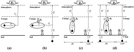
The description of the Penman-Monteith (P-M) model is given in Equation (1), and the model structure is shown in Figure 1a.

$$\lambda {\text{ET}}_{\text{a}}=\frac{\Delta \left(R_n-G\right)+\rho C_{\text{p}}D/r_a}{\Delta +\gamma \left[1+\left(r_c/r_a\right)\right]}$$

(1)

where λ is the latent heat of vaporization; R_n and G are net radiation and soil heat flux, respectively (W/m²); Δ is the slope of saturation vapor pressure—temperature curve (kPa/K), ρ is the air density (kg/m³), C_p is the specific heat of air at constant pressure (J/(kg K)), D is the vapor pressure deficit (kPa), γ is the psychrometric constant (kPa/K), r_a is aerodynamic resistance (s/m), and r_c is bulk surface resistance (s/m).

The aerodynamic resistance determines the transfer of heat and water vapor from evaporation surface into the air above the canopy, which is calculated from [35]

$$r_a=\frac{\text{ln}\left(\frac{z_m-d}{z_{om}}+{\phi }_{\text{M}}\right)\text{ln}\left(\frac{z_h-d}{z_{oh}}+{\phi }_{\text{H}}\right)}{k^{2}u\left(z_{\text{m}}\right)}$$

(2)

where k is von Karman’s constant (=0.41), d is zero plane displacement height (m), z_m and z_h are height of wind measurement and humidity measurement, respectively (m). u(z_m) is wind speed at height z_m (m/s), z_om is the roughness length governing momentum transfer, and z_oh is the roughness length governing heat and vapor transfer. Both roughness lengths (z_om, z_oh) and zero plane displacement height (d) are defined as functions of vegetation height (h), given in Campbell and Norman [36]. φ_M and φ_H represent atmospheric diabatic correction factors for momentum and heat (or vapor) respectively and can be found in [37].

The bulk surface resistance is estimated from [38]:

$$r_c=\frac{1}{2\mathit{LAI}}\frac{r_{\text{ST}\_\text{min}}}{f_1{f}_2{f}_3{f}_4}$$

(3)

where r_{ST_min} is the minimum stomatal resistance (s/m). f₁, f₂ and f₃ are factors accounting for the influence of shortwave radiation, air vapor deficit, and air temperature on stomatal resistance, respectively, and are estimated following Noilhan and Planton [39]. Parameter f₄ accounts for the influence of root zone soil moisture on stomatal resistance, which is calculated from

$$f_4(\theta )=\{\begin{array}{cc}0& \theta \le {\theta }_W\\ \frac{\theta -{\theta }_W}{{\theta }_F-{\theta }_W}& {\theta }_W<\theta <{\theta }_F\\ 1& {\theta }_F\le \theta \end{array}$$

(4)

where θ is the soil water content within the root-zone (cm³/cm³), θ_F and θ_W are the soil water content at the field capacity and wilting point, respectively.

2.1.2. Shuttleworth-Wallace Model

The Shuttleworth-Wallace (S-W) model is a typical two-layer model, which is also the basis of other multi-layer models. The model structure is shown in Figure 1b. In the S-W model, ET_a is calculated from,

$$\lambda {\text{ET}}_{\text{a}}=\lambda E+\lambda T=C_s{\mathit{PM}}_s+C_c{\mathit{PM}}_c$$

(5)

where λE is the latent heat from soil and λT is the latent heat from canopy (W/m²). Subscript s and c represent soil and canopy component, respectively. The expressions of PM and C are given by

$${\mathit{PM}}_s=\frac{\Delta A+\left[\rho C_{\text{p}}\text{D}-\Delta r_a^s\left(A-A_s\right)\right]/\left(r_a^a+r_a^s\right)}{\Delta +\gamma \left[1+(r_s^s/\left(r_a^a+r_a^s\right)\right]}$$

(6)

$${\mathit{PM}}_c=\frac{\Delta A+\left[\rho C_{\text{p}}\text{D}-\Delta r_a^c{A}_s\right]/\left(r_a^a+r_a^c\right)}{\Delta +\gamma \left[1+(r_s^c/\left(r_a^a+r_a^c\right)\right]}$$

(7)

$$C_c=1/\left(1+R_c{R}_a/R_s\left(R_c+R_a\right)\right)$$

(8)

$$C_s=1/\left(1+R_s{R}_a/R_c\left(R_s+R_a\right)\right)$$

(9)

$$R_a=(\Delta +\gamma )r_a^a$$

(10)

$$R_s=(\Delta +\gamma )r_a^s+\gamma r_s^s$$

(11)

$$R_c=(\Delta +\gamma )r_a^c+\gamma r_s^c$$

(12)

where $r_a^a$ is the aerodynamic resistance between mean canopy surface and the reference height (s/m); $r_a^s$ is the aerodynamic resistance between soil surface and mean canopy surface (s/m); $r_a^c$ is the aerodynamic resistance between mean leaf surface and mean canopy surface (s/m); $r_s^c$ is the canopy surface resistance, and $r_s^s$ is the soil surface resistance (s/m). A and A_s are the total available energy and the available energy for the soil component (W/m²), respectively, which can be estimated from

$$A=R_n-G$$

(13)

$$A_s=R_n\text{exp}\left(-k_c\mathit{LAI}\right)-G$$

(14)

where k_c is the extinction coefficient of radiation attenuation, and is set to be 0.7 for deciduous broadleaf forests, 0.5 for evergreen needle-leaf forests, and 0.4 for herbs [20,40].

The aerodynamic resistance $r_a^a$ and $r_a^s$ in the S-W model were assumed to change linearly between those for the surface with full vegetation cover (assumed equal to LAI = 4) and for bare soil, weighted by leaf area index [21]:

when 0 < LAI < 4

$$r_a^a=\frac{1}{4}\mathit{LAI}\times r_a^a(\alpha )+\frac{1}{4}(4-\mathit{LAI})\times r_a^a(0)$$

(15)

$$r_a^s=\frac{1}{4}\mathit{LAI}\times r_a^s(\alpha )+\frac{1}{4}(4-\mathit{LAI})\times r_a^s(0)$$

(16)

when LAI ≥ 4

$$r_a^a=r_a^a(\alpha )$$

(17)

$$r_a^s=r_a^s(\alpha )$$

(18)

where α and 0 in the bracket indicate full vegetation cover and bare soil, respectively.

Above the fully developed canopy, where the wind speed profile is logarithmic, the aerodynamic resistance $r_a^a$(α) is calculated using Equation (2). For aerodynamic resistance within the canopy, $r_a^s$ (α) is obtained by performing an integration of eddy diffusion coefficient (K) over the height from 0 to d + Z_om, i.e.,

$$r_a^s(\alpha )=\underset{0}{\overset{d+z_{om}}{\int }}\frac{dz}{K(z)}=\frac{\text{ln}\frac{z-d}{z_{om}}+{\phi }_{\text{M}}}{k^{2}u(z)}\frac{h}{n(h-d)}\left\{\text{exp}n-\text{exp}\left[n\left(1-\frac{d+z_{\text{m}}}{h}\right)\right]\right\}$$

(19)

where n is the extinction coefficient of the eddy diffusion, which is estimated by linear interpolation between the value for h < 1 m (=2.5) and h > 10 m (=4.25); u(z) is the wind speed at height z. The eddy diffusion coefficient K(z) is determined by

$$K(z)=\frac{k^2(h-d)u(z)}{\left[\text{ln}(z-d)/z_{om}\right]}\text{exp}[-n(1-z/h)]$$

(20)

For surface without canopy, $r_a^a$(0) and $r_a^s$(0) are estimated from the following equations without the consideration of the zero plane displacement height,

$$r_a^s(0)=\frac{\left(\text{ln}\frac{h}{{z_{om}}^{\prime }}+{\phi }_{\text{M}}\right)\left(\text{ln}\frac{h}{{z_{oh}}^{\prime }}{\phi }_{\text{H}}\right)}{k^{2}u(h)}$$

(21)

$$r_a^a(0)=\frac{\left(\text{ln}\frac{z_m}{{z_{om}}^{\prime }}+{\phi }_{\text{M}}\right)\left(\text{ln}\frac{z_h}{{z_{oh}}^{\prime }}{\phi }_{\text{H}}\right)}{k^{2}u(z_{\text{m}})}-r_a^s(0)$$

(22)

where z_om^′ and z_oh^′ are the roughness length of bare surface governing momentum transfer and heat and vapor transfer (=0.01 m) [41], respectively; u(h) is the wind speed at canopy height h

$$u(h)=\frac{\text{ln}\left[(h-d)/z_{om}\right]}{\text{ln}\left[(z_m-d)/z_{om}\right]}u\left(z_{\text{m}}\right)$$

(23)

The intra-canopy aerodynamic resistance $r_a^c$ is calculated from [42]

$$r_a^c=\frac{n}{0.02}\sqrt{\frac{l_w}{u(h)}}\frac{1}{1-e^{-n/2}}$$

(24)

where l_w is the characteristic length of leaf width (m) (

Table 1. General information of sites and selected model parameters used in this study.

Sites	Location a	Climate b	Vegetation	Vegetation c and Soil d Parameters	Study Period	Reference
US_MMS	W86.4131° N39.3232° a.s.l. 275 m	P = 1094 mm T = 10.8 °C	Deciduous Broad-leaf Forest	H = 27m, LAI = 0.84–4.72, Fr = 0.67–0.73, rST_min = 180 s/m, lw = 0.15 m, θF = 0.39, θW = 0.21	8 February 2003 to 13 November 2003	[49]
US_Fmf	W111.7273° N35.1426° a.s.l. 2160 m	P = 613 mm T = 11.4 °C	Woody Savannas	h = 18 m, LAI = 1.5, Fr = 0.3, rST_min = 180 s/m, lw = 0.02 m, θF = 0.41, θW = 0.086	1 February 2006 to 10 September 2006	[50]
US_Var	W120.9507° N38.4067° a.s.l. 129 m	P = 565 mm T = 16.9 °C	Grasslands	h = 0.2–0.55 m, LAI = 0.18–1.4, Fr = 1, rST_min = 130 s/m, lw = 0.03 m, θF = 0.28, θW = 0.07	10 January 2006 to 27 May 2006	[51]
US_Bo1	W88.2904° N40.0062° a.s.l. 219 m	P = 756 mm T = 11.4 °C	Croplands (Maize)	h = 0.22–2.32 m, LAI = 0.18–4.38, Fr = 0.1–0.9, rST_min = 130 s/m, lw = 0.03 m, θF = 0.33, θF = 0.1	24 May 2001 to 10 September 2001	[52]

^aDescription of the location for sites include longitude (W/E), latitude (N/S) and elevation above sea level (a.s.l.);^bDescription of climate condition for sites include annual average precipitation (P) and annual average air temperature (T). For US_MMS, P and T are averaged between 1971 and 2000; for US_Fmf, P and T are averaged between 2006 and 2010; for US_Var, P and T are averaged between 1946 and 2005; for US_Bo1, P is averaged between 1997 and 2006 and T is averaged between 1997 and 2007;^cThe value of Fr in the grassland site was assumed to be 100% during the main growing season (we found that Equation (29) is not applicable in grassland), which accords well with field survey, and the value of Fr for the forest and cropland sites were estimated from Equation (29). For the woody savannas site, the estimated values of Fr from Equation (29) were ranged from 0.26 to 0.29. However, according to the definition in the IGBP vegetation classification, the Fr of woody savannas should be between 0.3 and 0.6. As a result, a lower boundary of 0.3 was chosen for the woody savannas site;^dIn this study, θ_F was assumed to be the water content retained in the soil at −0.02 MPa of suction pressure, which is midway of most reported θ_F values (−0.01 to −0.033 MPa) [53]. θ_W was related to the suction pressure at −1.5 MPa. The VG-M model [54,55] was adopted to describe the soil water retention curve, and the parameters of the VG-M model for each site were estimated from measured soil texture and bulk density using the method given by [56].

).

The canopy surface resistance in the S-W model ( $r_s^c$) is similar with the bulk surface resistance in P-M model (r_c). Thus, $r_s^c$ can be computed from Equations (3) and (4). The soil surface resistance is computed using an empirical equation given by [43]

$$r_s^s=3.5{\left({\theta }_s/{\theta }_1\right)}^{2.3}+33.5$$

(25)

where θ₁ is the soil water content within the surface soil layer.

2.1.3. Two-Patch Model

In the two-patch (T-P) model (Figure 1c), both soil and vegetation components are assumed to receive full radiation loading, and the total flux of latent heat per unit area is calculated as the mean of fluxes from each component (canopy or soil) weighted by their relative areas [20]

$$\lambda {\text{ET}}_{\text{a}}=\mathit{Fr}\times \lambda T+(1-\mathit{Fr})\times \lambda E$$

(26)

$$\lambda T=\frac{\Delta A+\rho C_{p}D/\left(r_a^a+r_a^c\right)}{\Delta +\gamma \left[1+r_s^c/\left(r_a^a+r_a^c\right)\right]}$$

(27)

$$\lambda E=\frac{\Delta A+\rho C_{p}D/\left(r_a^a+r_a^s\right)}{\Delta +\gamma \left[1+r_s^s/\left(r_a^a+r_a^s\right)\right]}$$

(28)

where Fr is the fractional vegetation coverage. The value of Fr can be either determined by in situ measurements or estimated from remote sensing images (Table 1), in which Fr is calculated from [44]

$$F\text{r}=\left(\text{EVI}-{\text{EVI}}_{\text{min}}\right)/\left({\text{EVI}}_{\text{max}}-{\text{EVI}}_{\text{min}}\right)$$

(29)

where EVI is the enhanced vegetation index [45]; EVI_max and EVI_min are the maximum and minimum EVI values, respectively [46].

Aerodynamic resistances in the T-P model are similar with those in the S-W model. However, when calculating λE and λT, the T-P model assumes that transpiration occurs from a closed canopy surface while evaporation happens over bare soil. As a result, aerodynamic resistances $r_a^a$ and $r_a^c$ in Equation (27) are estimated by Equations (2) and (23), while those in Equation (28) are computed from Equations (21) and (22), respectively.

Lhomme and Chehbouni [20] suggested that for patchy or clumped vegetation, it is better to use the clumped leaf area index (L_c), which is defined as the LAI per unit vegetated area (L_c = LAI/F_r). Therefore, the bulk canopy surface resistance $r_s^c$is estimated from

$$r_s^c=\frac{1}{2L_{\text{c}}}\frac{r_{\mathit{ST}\_\text{min}}}{f_1{f}_2{f}_3{f}_4}$$

(30)

where r_{ST_min}, f₁, f₂, f₃, and f₄ keep the same meanings as those in P-M and S-W model.

Soil surface resistance of the T-P model is calculated from Equation (25).

2.2. Development of a Hybrid-Dual Source Model

The H-D model is a mixture of the layer approach and the patch approach (Figure 1d). It adopts the layer approach to allocate available energy between canopy and soil (Equation (14)) and to calculate aerodynamic resistances, and uses the patch approach to partition energy into latent heat (E or T), sensible heat (H), and ground heat flux (G). The energy balance equations are,

$$A_c=\mathit{Fr}\times \left(\lambda T+H_c\right)$$

(31)

$$A_s=(1-\mathit{Fr})\times \left(\lambda E+H_s\right)$$

(32)

For each component, fluxes of sensible and latent heat are calculated following the classical Ohm’s law type formulations. To account for environmental stresses on ET, the canopy and soil surface resistances were incorporated into the original hybrid dual-source potential ET model of Guan and Wilson [29],

$$H_c=\rho C_p\frac{\left(t_v-t_{zh}\right)}{r_a^c+r_a^a}$$

(33)

$$H_s=\rho C_p\frac{\left(t_s-t_{zh}\right)}{r_a^s+r_a^a}$$

(34)

$$\lambda T=\frac{\rho C_p}{\gamma }\frac{e_v-e_{zh}}{r_a^c+r_a^a+r_s^c}$$

(35)

$$\lambda E=\frac{\rho C_p}{\gamma }\frac{e_s-e_{zh}}{r_a^s+r_a^a+r_s^s}$$

(36)

where t and e are the air temperature and humidity, respectively. Subscript v represents the bulk leaf stomata and zh is the reference height where temperature and humidity are measured.

Assuming that vapor within the leaf stomata is always saturated under t_v, Equation (35) can be rewritten as

$$\lambda T=\frac{\rho C_p}{\gamma }\frac{e_{\mathit{sat}}\left(t_v\right)-e_{zh}}{r_a^c+r_a^a+r_s^c}$$

(37)

The term e_s in Equation (36) represents the equilibrium vapor pressure within the surface layer of soil, and can be calculated by the thermal equilibrium equation [47]. As a result, Equation (36) is rewritten as

$$\lambda E=\frac{\rho C_p}{\gamma }\frac{h_{\text{u}}{e}_{\mathit{sat}}\left(t_s\right)-e_{zh}}{r_a^s+r_a^a+r_s^s}$$

(38)

where parameter h_u is the relative humidity within the surface soil, and is estimated based on the assumption that water in the liquid and vapor phases are in local thermodynamic equilibrium [47]:

$$h_u=\text{exp}\left(\frac{g{h}_s}{R{t}_s}\right)$$

(39)

where R is the gas constant for water vapor (=461.5 J/(kg·K)); g is the gravitational acceleration (=9.8 m/s²); h_s and t_s are the water potential (m) and temperature (K) of the surface soil, respectively.

The Penman linear relationship [48] is employed to convert saturated vapor pressure at the reference height to that on the surface:

$$e_{\mathit{sat}}\left(t_v\right)=e_{\mathit{sat}}\left(t_{zh}\right)+\Delta \left(t_v-t_{zh}\right)$$

(40)

$$e_{\mathit{sat}}\left(t_s\right)=e_{\mathit{sat}}\left(t_{zh}\right)+\Delta \left(t_s-t_{zh}\right)$$

(41)

Substituting Equations (31), (33), (37) and (40), and convert fluxes into the total surface area, the canopy transpiration is calculated as:

$$\lambda T=\frac{\Delta A_c+\mathit{Fr}\frac{\rho C_p\left[e_{\mathit{sat}}\left(t_{zh}\right)-e_{zh}\right]}{r_a^a+r_a^c}}{\Delta +\gamma \left(1+\frac{r_s^c}{r_a^a+r_a^c}\right)}$$

(42)

Similarly, substituting Equations (32), (34), (38) and (41), one can get the expression for estimating soil evaporation,

$$\lambda E=\frac{h_u\Delta A_s+(1-\mathit{Fr})\frac{\rho C_p\left[h_u{e}_{\mathit{sat}}\left(t_{zh}\right)-e_{zh}\right]}{r_a^a+r_a^c}}{\Delta h_u+\gamma \left(1+\frac{r_s^s}{r_a^a+r_a^s}\right)}$$

(43)

Aerodynamic resistances ( $r_a^a$, $r_a^c$ and $r_a^s$) and soil surface resistance of the H-D model are calculated using the same equations as those of the S-W model. However, since the H-D model was originally proposed to estimate latent heat flux from non-uniform vegetation, the clumped leaf area index is used in the H-D model to upscale stomatal resistance into bulk canopy surface resistance ( $r_s^c$), as given in Equation (30).

3. Data and Evaluation Statistics for Models Being Examined

3.1. Study Site and Data

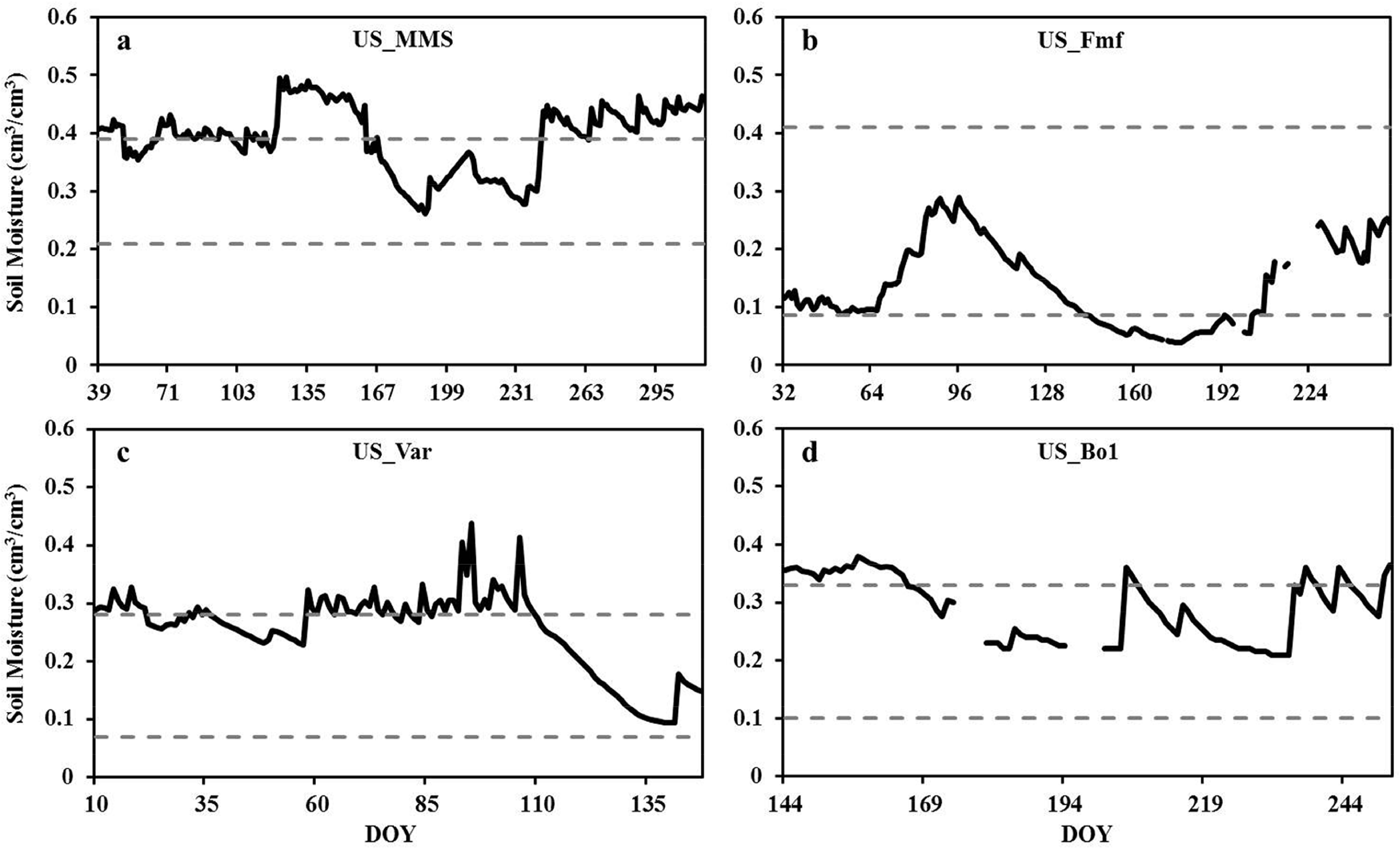
Four sites within the AmeriFlux network were used in this study to validate the model performance, including one deciduous broadleaf forest site (Morgan Monroe State Forest, US_MMS) [49], one woody savannas site (Flagstaff Managed Forest, US_Fmf) [50], one grassland site (Vaira Ranch, US_Var) [51], and one cropland site (Bondville, US_Bo1) [52]. For each site, continuous records of half-hourly meteorological and latent heat flux measurements from eddy covariance (EC) towers were obtained from the AmeriFlux Web site [53]. Ancillary and biological data include soil moisture and temperature, leaf area index (LAI) and vegetation height (h) were also acquired. A summary of the sites including locations, climate conditions, vegetation types, vegetation and soil parameters as well as study periods is listed in Table 1 [49–52,54–57], and soil moisture conditions during the study period for each site are shown in Figure 2.

Moderate Resolution Imaging Spectroradiometer (MODIS) images were used to estimate the EVI and then to calculate Fr (Equation (29)) for each site due to the lack of in situ Fr observations. EVI was calculated following the method given by [45] using MODIS surface reflectance dataset (MOD09GA) downloaded from the NASA Data Center [58]. The original MODIS images in the sinusoidal projection were re-projected into the UTM projection and resampled into 1 km spatial resolution. For days without measurements, the values of LAI, h and Fr were estimated by linearly interpolating those parameters between the two bounding observations.

It is worthwhile to mention that although EC measurements have been widely considered as the ground truth of energy and water exchanges between the land surface and the atmosphere, studies have shown that ET_a from EC system suffers from uncertainties to a certain degree, i.e., the energy balance closure of EC system generally lies between 80% and 95% [59]. In addition, linear interpolation of vegetation parameters during days without in situ measurements would also result in uncertainties. In this study, the EC-observed ET_a at the four sites was obtained from the level-4 AmeriFlux dataset, in which rigorous quality control procedures were made to guaranty the accuracy of EC observations [53]. Thus, ET_a from the EC system was regarded as ground truth of actual evapotranspiration to validate the four models in the following analysis.

3.2. Evaluation of Model Performance

Three statistic metrics recommend by Legates and McCabe [60] were used to evaluate the model performance, including the mean absolute error (MAE), the modified coefficient of efficiency (E₁), and the modified index of agreement (d₁):

$$\text{MAE}=N^{-1}\sum _{i=1}^N\left|O_i-S_{\text{i}}\right|$$

(44)

$$E_1=1.0-\frac{\sum _{i=1}^N\left|O_i-S_i\right|}{\sum _{i=1}^N\left|O_i-\overline{O}\right|}$$

(45)

$$d_1=1.0-\frac{\sum _{i=1}^N\left|O_i-S_i\right|}{\sum _{i=1}^N\left(\left|O_i-\overline{O}\right|+\left|S_i-\overline{O}\right|\right)}$$

(46)

where O_i is the observed value, S_i is the modeled value, and ō is the mean observed value. For a perfect model, MAE should be 0, and both E₁ and d₁ should be 1. A model performs better if MAE is smaller and E₁ and d₁ are lager.

In addition, the regressions of model estimated and observed ET with zero interception were also used to evaluate the model performance, i.e.,

$$\lambda {\text{ET}}_{\text{a}\_}\text{estimated}=a\lambda {\text{ET}}_{\text{a}\_\text{observed}}$$

(47)

where λET_a_model and λET_{a_}observed are model-estimated and observed ET_a, respectively, and a is the slope of regression. If a model performs well, the a value should be close to 1.

4. Results and Discussion

4.1. Validating the Performance of the Hybrid-Dual Source Model

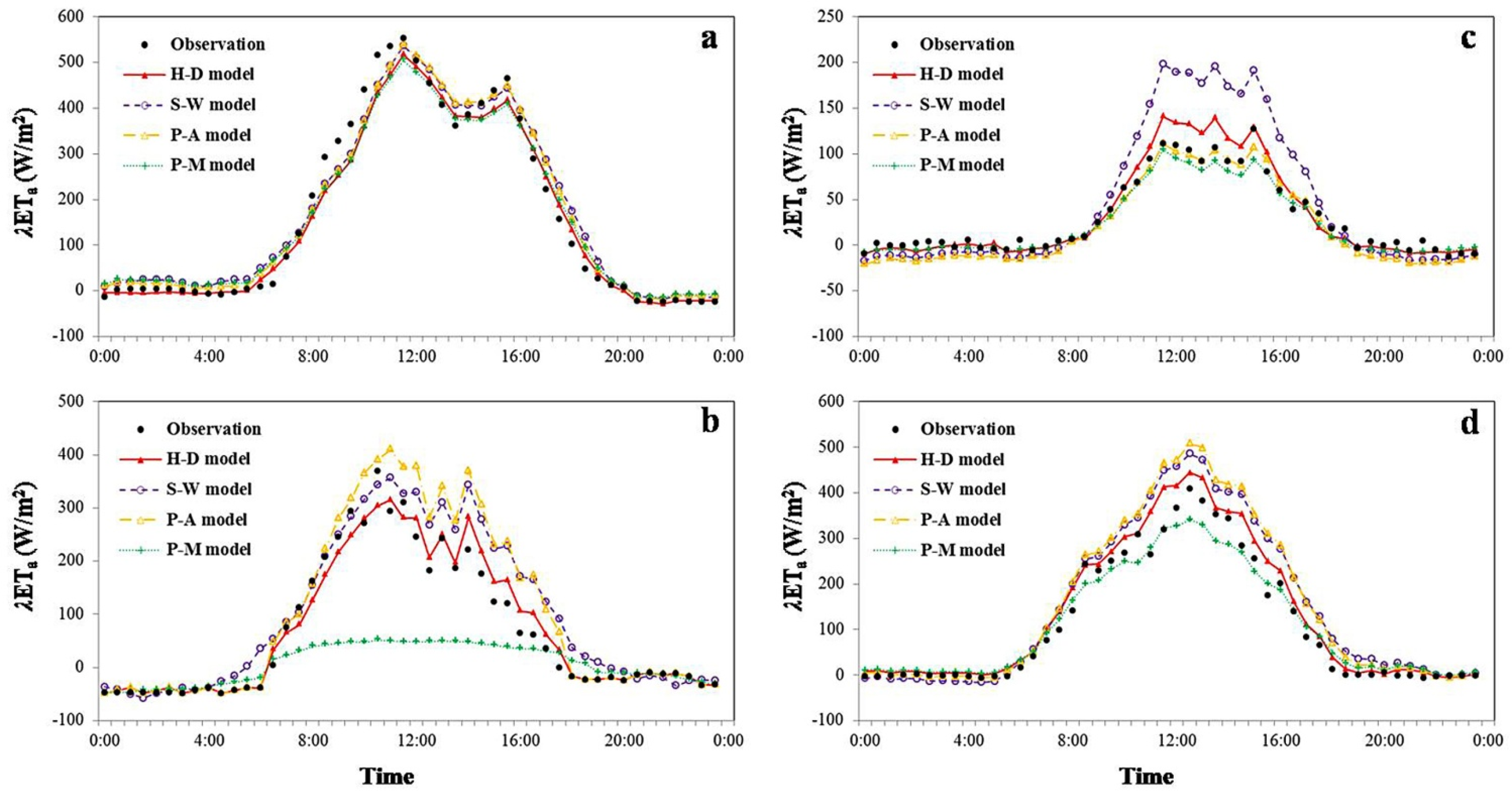
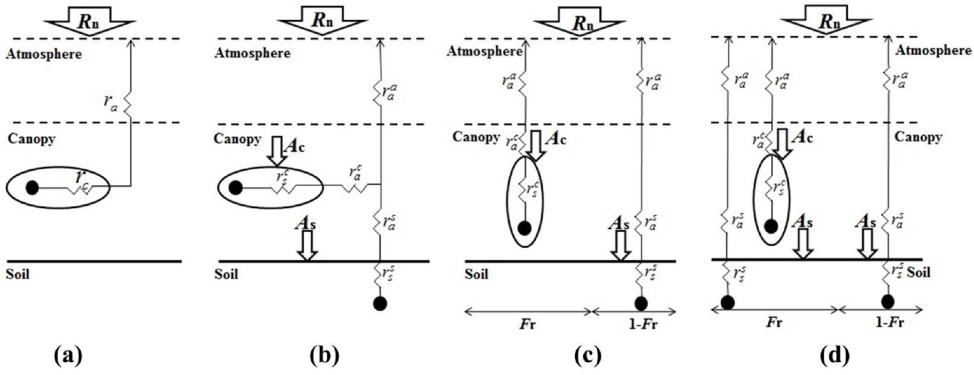
Performance of the H-D model in simulating ET_a at a 30-min interval was firstly validated with observations from the eddy covariance system (Figure 3a–d). Overall, the estimated ET_a agreed reasonably well with the ground-based measurements at all sites, with all fitted lines close to the 1:1 line. The MAE ranged from 16.3 to 38.6 W/m² (

Table 2. Statistic summary of the four models in estimating actual evapotranspiration over 30-min period at four sites. s̄ is the mean estimated value.

Sites	Models	ō (W/m2)	s̄ (W/m2)	MAE (W/m2)	E1	d1	α
US_MMS	H-D	115.7	113.5	37.6	0.72	0.87	0.95
	S-W	115.7	134.7	48.4	0.62	0.81	0.99
	T-P	115.7	126.3	42.9	0.64	0.82	0.98
	P-M	115.7	119.2	45.7	0.63	0.82	0.90
US_Fmf	H-D	131.5	125.7	38.6	0.56	0.77	0.89
	S-W	131.5	142.2	51.4	0.41	0.71	0.99
	T-P	131.5	163.1	53.2	0.38	0.72	1.15
	P-M	131.5	37.4	99.5	−0.20	0.43	0.20
US_Var	H-D	53.6	50.9	16.3	0.72	0.87	0.98
	S-W	53.6	76.7	33.8	0.37	0.75	1.40
	T-P	53.6	44.7	24.4	0.58	0.81	0.92
	P-M	53.6	43.4	15.7	0.73	0.86	0.93
US_Bo1	H-D	117.5	123.6	30.0	0.79	0.89	1.02
	S-W	117.5	137.2	34.9	0.71	0.86	1.12
	T-P	117.5	137.4	34.8	0.74	0.87	1.13
	P-M	117.5	105.9	34.4	0.74	0.86	0.87

), indicating good performance of the H-D model in all ecosystems being tested. The highest MAE occurred at the woody savannas site (Flagstaff Managed Forest, US_Fmf), with E₁ and d₁ for this site being 0.56 and 0.77, respectively. The lowest MAE appeared at the grassland site (Vaira Ranch, US_Var), with E₁ of 0.72 and d₁ of 0.87. For the deciduous broadleaf forest site (Morgan Monroe State Forest, US_MMS), the MAE was 37.6 W/m², E₁ 0.72, and d₁ 0.87. The cropland site (Bondville, US_Bo1) had the highest agreement between the estimated and observed ET, with d₁ of 0.89 and E₁ of 0.79.

ET_a has evident diurnal patterns as a result of combined physical (e.g., temperature and radiation diurnal variations) and biological (e.g., stomatal closure) factors. Generally, the H-D model successfully reproduced these diurnal patterns of ET_a at all sites (Figure 4). However, at the US_MMS and US_Fmf sites, the H-D model slightly underestimated ET in the morning and overestimated ET_a in the afternoon (Figure 4a,b). This discrepancy is likely due to a simple canopy interception algorithm for net radiation used in the model (see Equation (14)), which is not able to reflect the diurnal variation in the sunlight incident direction. In the H-D model, LAI was used to partition net radiation between soil and canopy (Equation (14)). However, the LAI value used here only corresponds to that when the sun was directly overhead. As the solar incident angle varies with time, the shadow area and therefore the “effective” LAI values can vary during the daytime. As a result, the use of Equation (14) would result in improper radiation partitioning especially when vegetation is tall (the mean vegetation height in US_MMS and US_Fmf are 27 m and 18 m, respectively (Table 1)) and the canopy structure is non-uniform. For the remaining two sites, the H-D model slightly overestimated ET_a during the daytime (Figure 4c,d). The overall good agreement between estimated and observed ET in different ecosystems indicates the potential of the H-D model to be applicable to a wide range of vegetated surfaces.

4.2. Comparison of Estimated Evapotranspiration by Four Models

To further demonstrate the advantages of the H-D model, four models with distinct treatments on vegetation characterization were compared in Figures 3 and 4 and Table 2. It is worthwhile to mention that the same set of parameters (as described in Section 2) was employed by the four models for each site; hence, disagreement among model performance is mainly caused by differences in model structures instead of different parameters. Interestingly, all statistics show that ET_a estimates from the H-D model show closer agreement with the measurements than those from three other models at all sites except for the P-M model at the US_Var site, where the value of E₁ of the P-M model was slightly higher than that of the H-D model (0.73 vs. 0.72) and the MAE of the P-M model was slightly lower than that of the H-D model (15.7 vs. 16.3 W/m²) (Table 2). The S-W and T-P models had similar performance at the US_MMS, US_Fmf and US_Bo1 sites, but the S-W model significantly overestimated ET_a at the US_Var site (Figure 3g). The P-M model showed the worst performance in estimating ET among the four models at the US_MMS and US_Fmf sites. However, it performed best at the US_Var site and better than the S-W model at the US_Bo1 site.

At the US_MMS site, the four models showed similar performance and corresponded well with measurements (Figure 3a,e,i,m and Figure 4a). The MAE ranged from 37.6 to 48.4 W/m² and the values of E₁ were all larger than 0.6 and d₁ were all larger than 0.8 (Table 2), indicating that all models appear to perform well at this site.

At the US_Fmf site, the P-M model severely underestimated ET_a with a slope of 0.20 and E₁ of −0.20, suggesting that the use of the P-M model to predict ET_a was even worse than using the mean value of the measurements (Figure 3n and Table 2). This marked underestimation was mainly because of the low Fr value at the site (around 0.3 during the study period), which failed to meet the assumption of “big leaf” in the P-M model. In addition, Stannard (1993) reported that the P-M model would underestimate ET when canopy surface resistance was much greater than soil surface resistance. During the study period, the average canopy surface resistance ( $r_s^c$) was about 560 s/m, while the average soil surface resistance ( $r_s^s$) was only 200 s/m at the US_Fmf site. Similar results can also be drawn from Figure 4b, where the P-M model greatly underestimated ET_a during the daytime. The performance of the three dual-source models is much better than that of the P-M model (Figure 3b,f,j,n, Figure 4b and Table 2), which can be ascribed mostly to their ability to discriminate plant transpiration from soil evaporation. However, the T-P model overestimated ET_a by about 24%, with E₁ of 0.38 and d₁ of 0.72, and the S-W model overestimated ET_a by 8%, with E₁of 0.41 and d₁ of 0.71 (Table 2). The low E₁ values of the T-P and S-W models suggest that both models do not seem to work at the woody savannas site.

For the grassland site (US_Var), where Fr was high and the vegetation distribution was relatively uniform, the performance of the P-M model was largely improved compared with that at the US_Fmf site (Figure 3c,g,k,o, Figure 4c and Table 2). The statistics show that the P-M model performed even better than the three dual-source models at this site (Table 2). The S-W overestimated ET_a by about 43% (the slope was 1.40), which is larger than results in published studies. Hu et al. [61] reported that the S-W model generally overestimated ET_a by 8%–15% at four grassland sites of similar latitude as the US_Var site. The T-P model also provided acceptable results, with a MAE of 24.4 W/m², E₁ of 0.58, and d₁ of 0.81.

The cropland site (US_Bo1) showed the best correlations between estimates and observations (Table 2) for all four models. In the farmland ecosystem where the soil moisture remains at high levels (e.g., due to irrigation), the P-M model with various bulk surface resistances was found to be a good predictor for evapotranspiration (Figures 3p and 4d and Table 2). This phenomenon has also been reported by other studies [32,33,62,63]. Figure 4d shows that the P-M model slightly underestimates ET_a during 10:00–14:00, with a MAE of 34.4 W/m², E₁ of 0.74, and d₁ of 0.86 for the study period (Table 2). Amongst the dual-source models being tested, the ET_a estimates from the S-W and T-P models have almost the same diurnal patterns (Figure 4d) and similar statistic values (Table 2), suggesting that these two models can be interchangeably used to estimate ET_a at the cropland site.

4.3. Evapotranspiration Components (E and T) and its Vegetation Controls

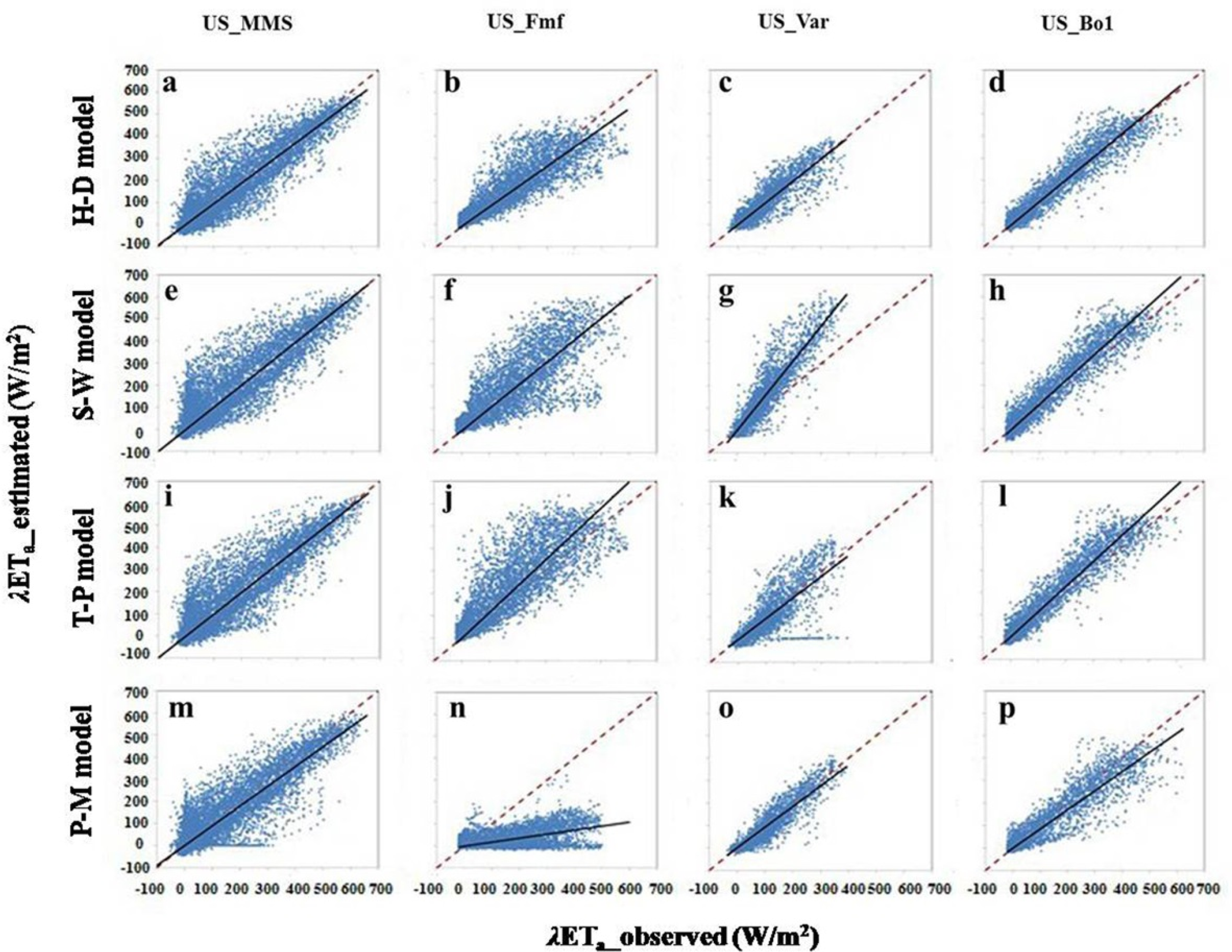
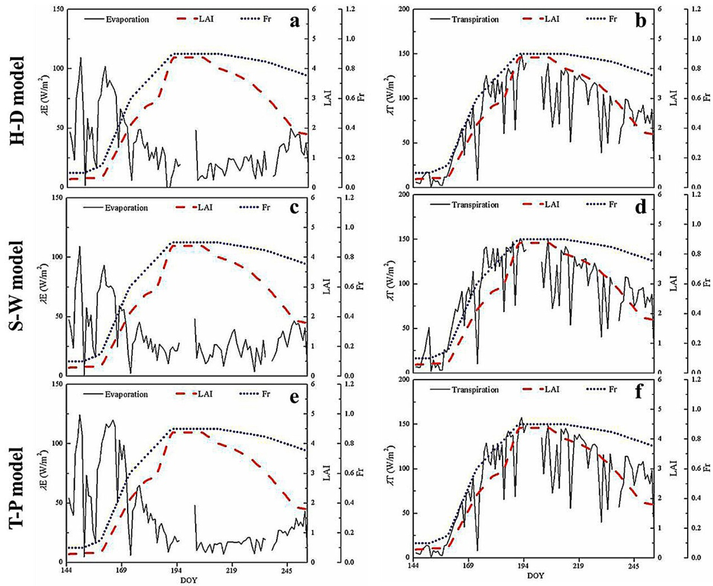
Differing descriptions of vegetation coverage characteristics are the largest difference among the four ET_a models. In order to trace the error of ET_a estimates and explore the underlying reasons, variations in daily LAI, Fr, and estimated daily evaporation (E) and transpiration (T) from the three dual-source models at four sites are shown in Figures 5 and 8. A summary of mean evaporation, mean transpiration, and the ratio of E/ET_a during study periods from each model is given in

Table 3. Summary of mean evaporation (E, W/m²), mean transpiration (T, W/m²), and the ratio of E/ET (%) at four sites during study periods.

Model	US_MMS			US_Fmf			US_Var			US_Bo1
	E	T	E/ETa	E	T	E/ETa	E	T	E/ETa	E	T	E/ETa
H-D	26.1	87.4	23.0	104.1	21.6	82.8	29.7	21.9	57.6	37.3	86.3	30.2
S-W	32.4	102.3	24.1	110.7	31.5	77.8	34.5	42.2	45.0	39.5	97.7	28.8
T-P	53.1	73.2	42.0	132.7	30.4	81.3	0	44.7	0	43.8	93.6	31.9

. Due to the inability to distinguish E and T, the P-M model was precluded from the following analysis.

At the US_MMS site where LAI varied markedly and soil moisture remains relatively constant at a high level (favorable water conditions, Figure 2a) during the study period, variations in transpiration from the H-D model show an obvious positive relationship with those in LAI, whereas evaporation is negatively correlated with LAI (Figure 5a,b). Similar relationships were also found for the S-W model (Figure 5c,d). However, both E and T from the T-P model did not show obvious variation with changes in LAI. This is because LAI is not used in the T-P model, while Fr is the only variable used to account for the vegetation controls on E and T partitioning. During the study period, Fr remained nearly invariant. As a result, both E and T from the T-P model show dampened variations compared with those from the H-D and S-W models (Figure 5e,f).

The ratio of E/ET_a was similar between the H-D and the S-W models (Table 3). However, the S-W model predicted higher values of both E and T compared with the H-D model. Given the fact that the H-D model accurately estimated the total ET_a while the S-W model overestimated it (Figure 3a,e, Figure 4a and Table 2), it is plausible that both E and T were overestimated in the S-W model. Similarly, the E/ET_a ratio from the T-P model was much higher than that from the H-D model, suggesting that the T-P model overestimated E and underestimated T at this site (Table 3).

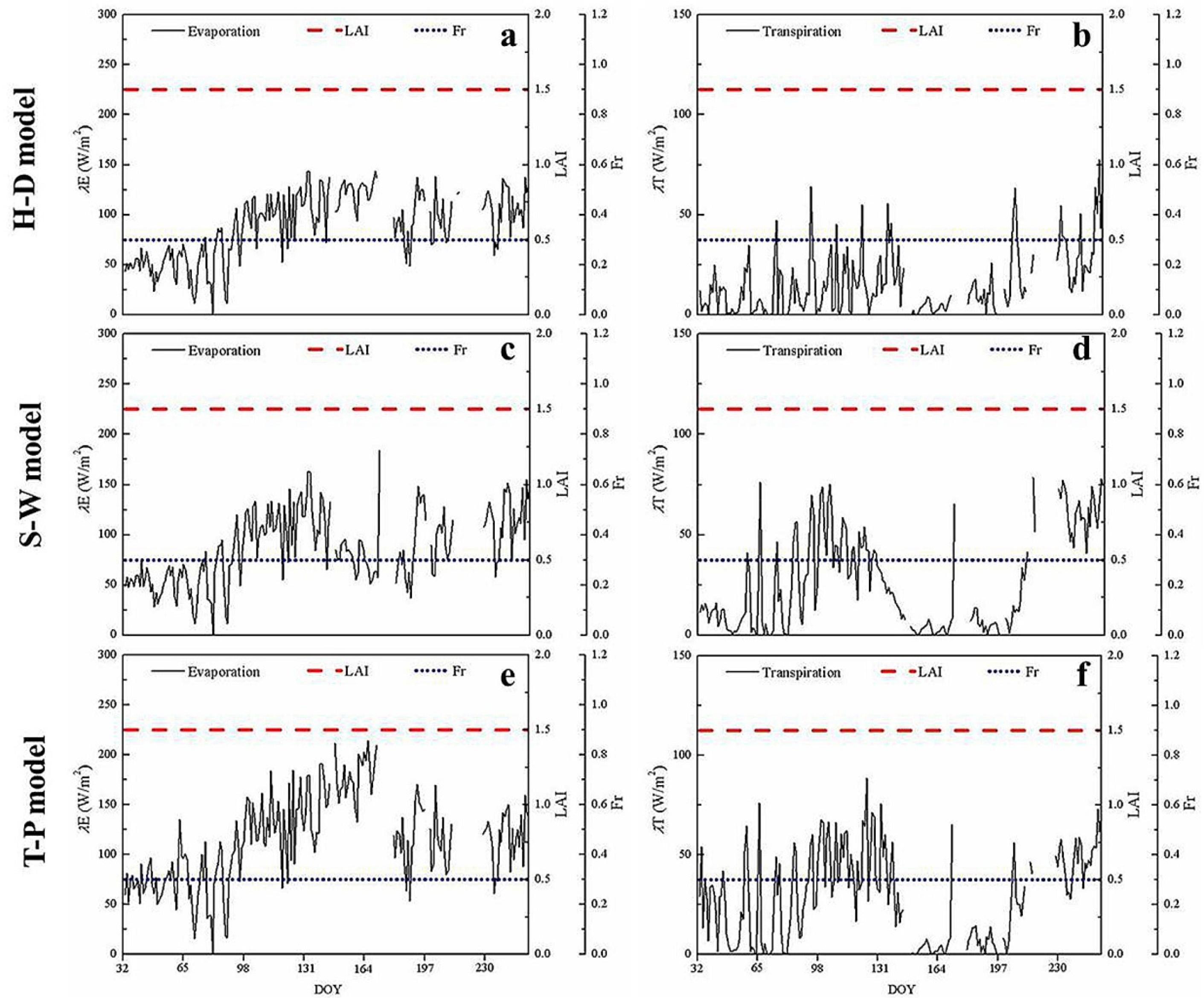
At the US_Fmf site, both LAI and Fr remained generally invariant during the simulation period. Variations in E and T were therefore controlled primarily by atmospheric and soil moisture conditions. It is observed that T from the three models showed similar trends that appear to increase before ∼DOY 130 and then to decrease to a low level between ∼DOY 140 and ∼DOY 210. Afterwards, T started to increase again. This trend corresponds well with that of soil moisture shown in Figure 2b, suggesting a strong moisture control on plant transpiration at this site. Although the surface vegetation condition was not the influential factor controlling seasonal variations in E and T, it does play a key role in partitioning ET_a into E and T. Because both the LAI and Fr were small at this site, E accounted for a larger proportion of total ET (Table 3). The ratio of E/ET_a was the highest from the H-D model (82.8%) and lowest from the S-W model (77.8%). For the T-P model, the E/ET_a ratio was 81.3%. Combining the results listed in Tables 2 and 3, it was found that the S-W model overestimated T but the proposed H-D model underestimated T. In addition, both E and T were significantly overestimated by the T-P model.

At the US_Var site, LAI showed obvious seasonal variations while Fr remained invariant. Evaporation from both the H-D and S-W models had similar values (Table 3) and remained relatively constant despite changes in LAI. This is possibly because that the actual evaporation process at this site was controlled mostly by the variability in meteorological and soil moisture conditions. During the study period, atmospheric demand was expected to increase with time, and soil moisture remained at a high level before ∼DOY 100 but showed an abrupt decrease afterwards (Figure 2c), which may somehow offset the increase in atmospheric demand and result in a relatively unchanged evaporation rate. Such an effect could also affect the process of transpiration. However, T from the S-W model exhibited a sharp increase after ∼DOY 100 despite the reduction in soil moisture (Figure 7d), resulting in a higher/lower T/E ratio in the S-W model (i.e., E/ET_a = 45%). In contrast, T from the H-D model that shows a more gradual increase with LAI after ∼DOY 100 seems to be more reasonable (Figure 7b). The above phenomenon suggests that the S-W model may respond to changes in LAI/soil moisture more/less sensitively than the H-D model does. Considering that the H-D model estimated total ET_a more precisely while the S-W model considerably overestimated the total ET_a (Table 2), and both models predicted similar E (Table 3), it could be derived that the S-W model overestimated the T at this site. Studies also reported that the ratio of E/ET_a for the grassland with mean growing season LAI of 0.50 (close to 0.52 of the US_Var site) were between 56% and 60% [61], which lends credibility to our findings at the US_Var site.

As for the T-P model, because the site was completely covered by vegetation, there was no evaporation occurred during the simulation period (Figure 7e). It is interesting to note that the negligible E was well compensated by the overestimation of T due to higher canopy available energy, thereby resulting in comparable total ET_a estimates (Table 2). However, because of the obviously erroneous E and T partitioning, it is not recommended using the T-P model at the site.

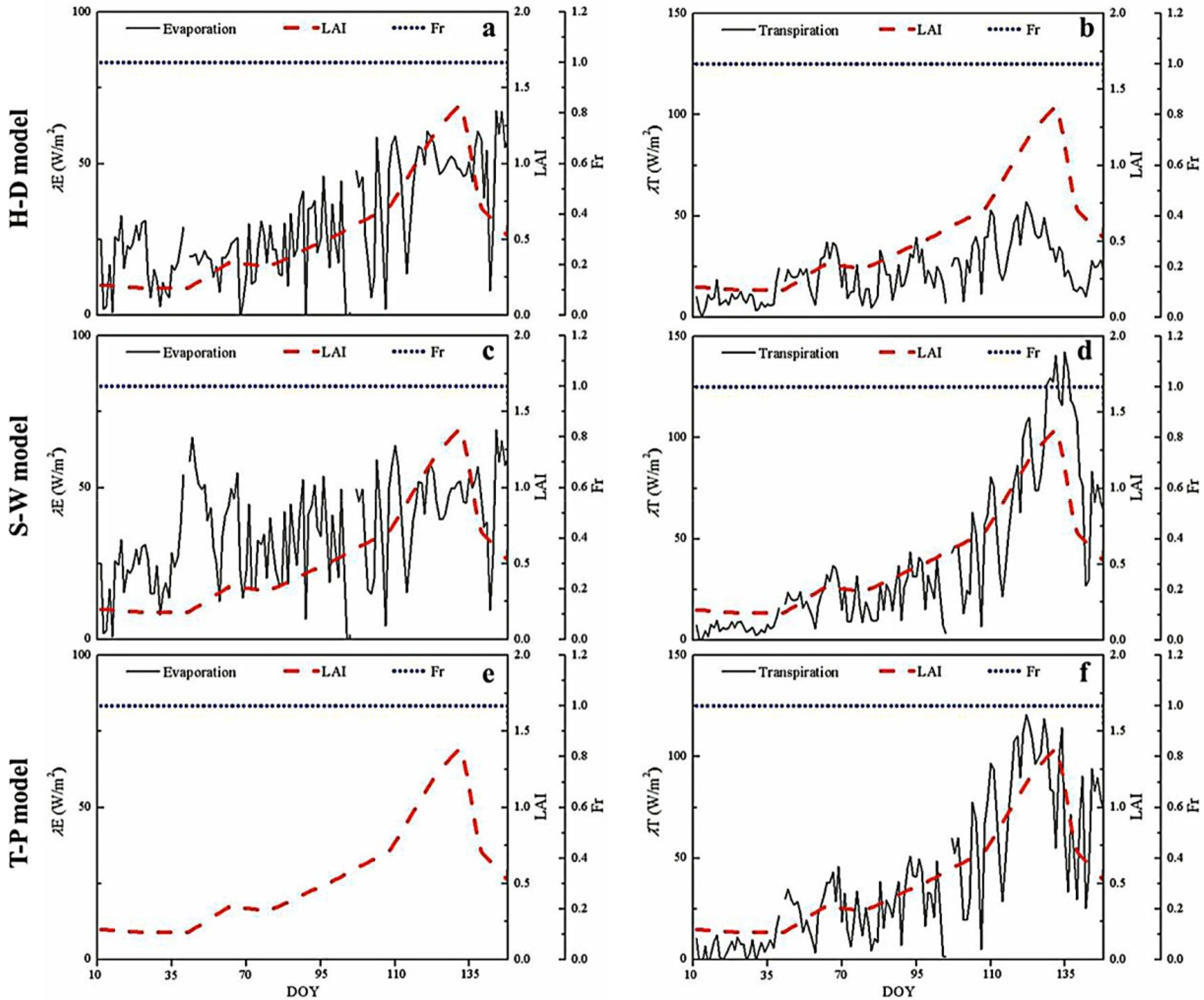
At the US_Bo1 site, soil moisture remained at a high level (Figure 2c) and both LAI and Fr changed synchronously during most of the simulation period (Figure 8). As a result, both E and T estimated by all three models showed similar temporal patterns. The estimated transpiration was positively correlated with changes in LAI and Fr, while the evaporation was negatively related with these two variables. In addition, the three models had similar E/ET_a ratios, with values ranging from 28.8% to 31.9% (Table 3). However, the S-W and T-P models slightly overestimated T compared to the H-D model (Table 3). This overestimation of transpiration would likely be as a result of the overestimation in total ET by these two models (Table 2). Nevertheless, the overestimation of the S-W model happened mostly during the beginning and the end of the simulation period when LAI was generally low (Figure 8b,d), whereas the overestimation of the T-P model mainly occurred in the end of the simulation period with low LAI but high Fr values.

Similar results can also be found at three other sites that the S-W model tended to overestimate T when LAI was low, and therefore overestimated the total ET_a. Conceptually, this is because the S-W model assumes fluxes from different components to be firstly fully coupled and then interact with the above atmosphere. However, when LAI is low, the interactions between fluxes from different components become less intense, which may contradict the assumption of the S-W model. This discrepancy would be even larger if Fr is also small. Other similar studies also reported that the S-W model overestimated T under low LAI conditions [26,29,61].

In contrast, the T-P model does not consider LAI. Instead, it uses Fr to partition available energy and to rescale latent fluxes between components. As a result, the T-P model provided a relatively high transpiration rate under high Fr conditions regardless of low LAI values. This phenomenon was not only found at the US_Bo1 site but also at the US_MMS and US_Var sites (Figures 5 and 6).

4.4. Advantages of the Hybrid Dual-Source Model

Compared with the S-W and T-P models, the estimated E and T from the H-D model seem more reasonable. Not surprisingly, the H-D model performed best in estimating total ET_a (Table 2). The H-D model deviates from a layer model in distinguishing the difference in evaporation from inter-canopy soil and that from under-canopy soil, and restricting convective transfer contributions to transpiration only from vegetated fractions. The H-D model is also different from a patch model in that it allows E from under-canopy soil, and the effect of vegetation on both E and T is somehow considered. More importantly, both LAI and Fr are adopted in the H-D model, while the S-W model only uses the LAI and the T-P model only uses the Fr. It should be emphasized that LAI and Fr are two variables representing different characteristics of surface vegetation distribution. LAI focuses on the vertical density and distribution of leaves, whereas Fr explains more on the horizontal development of vegetation canopies. Therefore, both variables showed strong, but different controls on E and T processes (Figures 5 and 8, see also Yang and Shang [13,64]). Although the value of both variables would change synchronously in some situations (i.e., in the farmland ecosystem, and thus resulted in similar E and T estimation among three dual-source models (Figure 8)), they function differently in determining ET_a processes. Moreover, synchronized changes in LAI and Fr rarely happen in natural ecosystems.

5. Implications for Satellite-Based ET Modeling Approaches

Since the late 1970s, satellite remote sensing has been widely used in ET_a modeling by providing critical variables depicting characteristics and the state of the land surface, e.g., land surface temperature and Fr. The basis of satellite-based ET_a modeling approaches is reliant on physical and mathematical description and/or simplification of the interactions of water and heat fluxes between vegetation and soil components. Overall, there are two ways to make use of satellite-based retrievals of surface and/or atmospheric variables to simulate ET_a from field to continental scales based on approaches entailing different assumptions, configurations, and coupling between vegetation and soil.

The first way is to mainly use remotely sensed Fr to describe composite components of the land surface and parameterize E and T separately based on the Penman-Monteith equation and T-P approach [44,46,65–67]. Furthermore, remotely sensed vegetation indices (e.g., EVI or the Normalized Difference Vegetation Index, NDVI) are physically and mathematically related to parameters associated with soil moisture stress on ET_a and surface resistance. Based on this framework, there are two valuable global ET_a products developed based on the Moderate Resolution Imaging Spectroradiometer (MODIS) [44] or NOAA-Advanced Very High Resolution Radiometer (AVHRR) [68]. These products take advantages of multispectral reflectance that shows relatively slow variations compared with land surface temperature and are therefore less compromised by cloud contamination. However, as indicated by more recent studies by Long et al. [4,69], Ruhoff et al. [70], and Yang et al. [71], these global satellite ET_a products or vegetation indices-based ET_a output show a slower response to precipitation and soil moisture in some cases compared with hydrological models, especially during extremely dry or wet conditions. This could be related to an indirect relationship between remotely sensed vegetation index and soil moisture but a more dynamic response of ET_a to soil moisture is explicitly depicted and simulated in hydrological models [72]. One of the most important strengths of satellite ET_a products is its relatively high spatial resolution (∼1–8 km) compared with the coarse resolution of hydrological models (e.g., 1/8 degree, ∼14 km at the equator). The global ET_a products could be valuable in interpreting ET_a patterns on a global scale and large river basin scales.

The second way is to use remotely sensed land surface temperature as a primary forcing of models to integrally or separately simulate sensible heat fluxes of vegetation and soil. Latent heat fluxes are subsequently calculated as the residual of the energy balance. Examples of single-source models of this approach include the Surface Energy Balance Algorithm for Land (SEBAL) [73], the modified-SEBAL [3], and the Surface Energy Balance System [74]. In addition, some of these single-source models suffer somewhat from subjectivity and uncertainty due to manual selection of end-members that reflect ET_a under extreme conditions from satellite images. These issues have been systematically investigated recently [6,75,76]. The dual-source models seem to be able to more realistically depict the interactions of turbulent fluxes between vegetation and soil components. Examples of dual-source models include the series Two Source Energy Balance (S-TSEB) and patch TSEB (P-TSEB) [11,12,77]. Based on the H-D scheme developed in the presented study, decomposition of composite remotely sensed radiative temperature into temperature components based on a trapezoid framework [78,79], soil moisture isoplethes [80–83], and interpolating slopes of dry and wet edges for inferring slopes of soil moisture isoplethes [84], a Hybrid dual-source scheme and Trapezoid framework based ET Model (HTEM) has been developed and showed a favorable accuracy in central Iowa in the US and the North China Plains [13]. In this way, the requirement for air temperature and vapor pressure involved in the H-D model that are not readily available through satellite remote sensing is circumvented but the advantages of the two-layer and two-source schemes are retained.

There is always a tradeoff between data requirement, model complexities and uncertainties, as well as purposes of studies and applications. Many satellite-based models were developed with the intention to reduce parameters and forcing data so as to be applicable over large heterogeneous areas [85,86]. We propose that for global change studies, use of ET_a models/products with the law of parsimony and simplicity is necessary. Therefore, incorporating remotely sensed vegetation indices as was done by MODIS and AVHRR ET_a products is feasible and should be very useful on global and continental scales. However, for regional, watershed, and field scales, use of H-D scheme-based approaches by incorporating more or less a priori knowledge and information on soil (e.g., soil surface albedo and emissivity) and vegetation (e.g., vegetation height) is necessary and should be able to provide more realistic partitioning between E and T as shown in this study and others [62].

Furthermore, satellite remote sensing can also provide surface albedo that is extremely critical to determining energy budgets of the land surface and therefore ET_a [5,87]. Parameterization schemes of net radiation and its components (e.g., shortwave and longwave radiation) and land cover classification keep evolving and should greatly benefit satellite-based ET_a modeling in the future [88–91]. It should be further emphasized that the four models we examined in this study are not the only models of their type in existence, and adding complexity to a model of this type does not necessarily improve it, although in this case the additional components such as the inclusion of LAI did add benefit.

6. Conclusions

In this study, a hybrid dual source (H-D) model is developed and applied in four different ecosystems to estimate actual ET processes. Outputs of the H-D model were tested against eddy covariance measurements and compared with three other ET models. The results indicate that: (1) the H-D model could generate accurate ET estimates in different ecosystems, with mean absolute errors ranging from 16.3 W/m² to 38.6 W/m², modified coefficient of efficiency ranging from 0.56 to 0.79, and modified index of agreement ranging from 0.48 to 0.87; (2) the H-D model generally gives better ET estimates and E and T partitioning than the three other models (i.e., MAE = 33.8∼51.4 W/m² for the S-W model, MAE = 24.4∼53.2 W/m² for the T-P model and MAE = 15.7∼99.5 W/m² for the P-M model), suggesting that the H-D model appear to be more suited for ET_a estimation over surfaces with different vegetation patterns; (3) the P-M model significantly underestimates ET_a in the savannas ecosystem (i.e., MAE = 99.5 W/m²), but generally performs well in other three ecosystems; and (4) the S-W model tends to overestimate plant transpiration when LAI is low, and the T-P model tends to overestimate plant transpiration under low LAI but high Fr conditions. This study could provide guidance on the use of satellite-based retrievals in different ET_a modeling approaches in the future.

References

- Oki, T.; Kanae, S. Global hydrological cycles and world water resources. Science 2006, 313, 1068–1072. [Google Scholar]
- Betts, A.K.; Ball, J.H.; Beljaars, A.C.M.; Miller, M.J.; Viterbo, P.A. The land surface-atmosphere interaction: A review based on observational and global modeling perspectives. J. Geophys. Res.: Atmos 1996, 101, 7209–7225. [Google Scholar]
- Xia, Y.L.; Mitchell, K.; Ek, M.; Cosgrove, B.; Sheffield, J.; Luo, L.F.; Alonge, C.; Wei, H.L.; Meng, J.; Livneh, B.; et al. Continental-scale water and energy flux analysis and validation for north American land data assimilation system project phase 2 (NLDAS-2): 2. Validation of model-simulated streamflow. J.Geophys. Res.: Atmos 2012, 117. [Google Scholar] [CrossRef]
- Long, D.; Longuevergne, L.; Scanlon, B.R. Uncertainty in evapotranspiration from land surface modeling, remote sensing, and GRACE satellites. Water Resour. Res 2014, 50, 1131–1151. [Google Scholar]
- Long, D.; Singh, V.P. Integration of the GG model with SEBAL to produce time series of evapotranspiration of high spatial resolution at watershed scales. J. Geophys. Res.: Atmos 2010, 115, D21128. [Google Scholar]
- Long, D.; Singh, V.P. Assessing the impact of end-member selection on the accuracy of satellite-based spatial variability models for actual evapotranspiration estimation. Water Resour. Res 2013, 49, 2601–2618. [Google Scholar]
- Yang, Y.T.; Shang, S.H.; Jiang, L. Remote sensing temporal and spatial patterns of evapotranspiration and the responses to water management in a large irrigation district of north China. Agric. Forest Meteorol 2012, 164, 112–122. [Google Scholar]
- Domingo, F.; Villagarcia, L.; Brenner, A.J.; Puigdefabregas, J. Evapotranspiration model for semi-arid shrub-lands tested against data from SE Spain. Agric. For. Meteorol 1999, 95, 67–84. [Google Scholar]
- McCabe, M.F.; Wood, E.F. Scale influences on the remote estimation of evapotranspiration using multiple satellite sensors. Remote Sens. Environ 2006, 105, 271–285. [Google Scholar]
- Anderson, M.C.; Norman, J.M.; Mecikalski, J.R.; Otkin, J.A.; Kustas, W.P. A climatological study of evapotranspiration and moisture stress across the continental united states based on thermal remote sensing: 1. Model formulation. J. Geophys. Res.: Atmos 2007, 112, D10117. [Google Scholar]
- Norman, J.M.; Anderson, M.C.; Kustas, W.P.; French, A.N.; Mecikalski, J.; Torn, R.; Diak, G.R.; Schmugge, T.J.; Tanner, B.C.W. Remote sensing of surface energy fluxes at 101-m pixel resolutions. Water Resour. Res 2003, 39. doi: 10.1029.2002WR001775. [Google Scholar]
- Norman, J.M.; Kustas, W.P.; Humes, K.S. A two-source approach for estimating soil and vegetation energy fluxes in observations of directional radiometric surface-temperature. Agric. For. Meteorol 1995, 77, 263–293. [Google Scholar]
- Yang, Y.; Shang, S. A hybrid dual-source scheme and trapezoid framework-based evapotranspiration model (HTEM) using satellite images: Algorithm and model test. J. Geophys. Res 2013, 118, 2284–2300. [Google Scholar]
- Zhao, L.; Xia, J.; Sobkowiak, L.; Li, Z. Climatic characteristics of reference evapotranspiration in the Hai River basin and their attribution. Water 2014, 6, 1482–1499. [Google Scholar]
- Francone, C.; Cassardo, C.; Spanna, F.; Alemanno, L.; Bertoni, D.; Richiardone, R.; Vercellino, I. Preliminary results on the evaluation of factors influencing evapotranspiration processes in vineyards. Water 2010, 2, 916–937. [Google Scholar]
- Monteith, J.L. Evaporation and environment. Symp. Soc. Exp. Biol 1965, 19, 205–234. [Google Scholar]
- Verhoef, A.; DeBruin, H.A.R.; VandenHurk, B.J.J.M. Some practical notes on the parameter kB−1 for sparse vegetation. J. Appl. Meteorol 1997, 36, 560–572. [Google Scholar]
- Yang, Y.T.; Shang, S.H.; Guan, H.D. Development of a soil-plant-atmosphere continuum model (HDS-SPAC) based on hybrid dual-source approach and its verification in wheat field. Sci. China Technol. Sci 2012, 55, 2671–2685. [Google Scholar]
- Lynn, B.H.; Carlson, T.N. A stomatal-resistance model illustrating plant vs. external control of transpiration. Agric. For. Meteorol 1990, 52, 5–43. [Google Scholar]
- Lhomme, J.P.; Chehbouni, A. Comments on dual-source vegetation-atmosphere transfer models. Agric. For. Meteorol 1999, 94, 269–273. [Google Scholar]
- Shuttleworth, W.J.; Wallace, J.S. Evaporation from sparse crops—An energy combination theory. Q. J. R. Meteor. Soc 1985, 111, 839–855. [Google Scholar]
- Blyth, E.M.; Harding, R.J. Application of aggregation models to surface heat-flux from the sahelian tiger bush. Agric. For. Meteorol 1995, 72, 213–235. [Google Scholar]
- Zhang, B.Z.; Kang, S.Z.; Li, F.S.; Zhang, L. Comparison of three evapotranspiration models to bowen ratio-energy balance method for a vineyard in an and desert region of northwest China. Agric. For. Meteorol 2008, 148, 1629–1640. [Google Scholar]
- Breshears, D.D.; Ludwig, J.A. Near-ground solar radiation along the grassland-forest continuum: Tall-tree canopy architecture imposes only muted trends and heterogeneity. Austral. Ecol 2010, 35, 31–40. [Google Scholar]
- Lhomme, J.P.; Montes, C.; Jacob, F.; Prevot, L. Evaporation from heterogeneous and sparse canopies: On the formulations related to multi-source representations. Bound. Lay. Meteorol 2012, 144, 243–262. [Google Scholar]
- Brenner, A.J.; Incoll, L.D. The effect of clumping and stomatal response on evaporation from sparsely vegetated shrublands. Agric. For. Meteorol 1997, 84, 187–205. [Google Scholar]
- Gu, L.H.; Shugart, H.H.; Fuentes, J.D.; Black, T.A.; Shewchuk, S.R. Micrometeorology, biophysical exchanges and nee decomposition in a two-story boreal forest—Development and test of an integrated model. Agric. For. Meteorol 1999, 94, 123–148. [Google Scholar]
- Lhomme, J.P.; Montes, C.; Jacob, F.; Prevot, L. Evaporation from multi-component canopies: Generalized formulations. J. Hydrol 2013, 486, 315–320. [Google Scholar]
- Guan, H.; Wilson, J.L. A hybrid dual-source model for potential evaporation and transpiration partitioning. J. Hydrol 2009, 377, 405–416. [Google Scholar]
- Seneviratne, S.I.; Corti, T.; Davin, E.L.; Hirschi, M.; Jaeger, E.B.; Lehner, I.; Orlowsky, B.; Teuling, A.J. Investigating soil moisture-climate interactions in a changing climate: A review. Earth Sci. Rev 2010, 99, 125–161. [Google Scholar]
- Jung, M.; Reichstein, M.; Ciais, P.; Seneviratne, S.I.; Sheffield, J.; Goulden, M.L.; Bonan, G.; Cescatti, A.; Chen, J.Q.; de Jeu, R.; et al. Recent decline in the global land evapotranspiration trend due to limited moisture supply. Nature 2010, 467, 951–954. [Google Scholar]
- Ortega-Farias, S.; Olioso, A.; Antonioletti, R.; Brisson, N. Evaluation of the penman-monteith model for estimating soybean evapotranspiration. Irrig. Sci 2004, 23, 1–9. [Google Scholar]
- Ortega-Farias, S.O.; Olioso, A.; Fuentes, S.; Valdes, H. Latent heat flux over a furrow-irrigated tomato crop using penman-monteith equation with a variable surface canopy resistance. Agric. Water Manag 2006, 82, 421–432. [Google Scholar]
- Massman, W.J. A surface-energy balance method for partitioning evapotranspiration data into plant and soil components for a surface with partial canopy cover. Water Resour. Res 1992, 28, 1723–1732. [Google Scholar]
- Allen, R.G.; Pereira, L.S.; Raes, D.; Smith, M. Crop Evapotranspiration-Guidelines for Computing Crop Water Requirements; FAO Irrigation and Drainage Paper 56; United Nations Food and Agriculture Organization: Rome, Italy, 1998. [Google Scholar]
- Campbell, G.S.; Norman, J.M. An Introduction to Environmental Biophysics; Springer: New York, NY, USA, 1998. [Google Scholar]
- Brutsaert, W. Evaporation into the Atmosphere: Theory, History and Applications; Reidel, D., Ed.; Springer: Dordrecht, The Netherlands, 1982. [Google Scholar]
- Jarvis, P.G. Interpretation of variations in leaf water potential and stomatal conductance found in canopies in field. Phil. Trans. R. Soc. B 1976, 273, 593–610. [Google Scholar]
- Noilhan, J.; Planton, S. A simple parameterization of land surface processes for meteorological models. Mon. Weather Rev 1989, 117, 536–549. [Google Scholar]
- Monsi, M.; Saeki, T. Uber den lichtfaktor in den pflanzengesellschaften und seine bedeutung fur die stoffproduktion. Jpn. J. Bot 1953, 14, 22–52. [Google Scholar]
- Van Bavel, C.H.M.; Hillel, D.I. Calculating potential and actual evaporation from a bare soil surface by simulation of concurrent flow of water and heat. Agric. Meteorol 1976, 17, 453–476. [Google Scholar]
- Choudhury, B.J.; Monteith, J.L. A 4-layer model for the heat-budget of homogeneous land surfaces. Q. J. Roy. Meteor. Soc 1988, 114, 373–398. [Google Scholar]
- Lin, J.D.; Sun, S.F. A study of moisture and heat transport in soil and the effect of resistance to evaporation. J. Hydrol. Eng 1983, 14, 1–8. [Google Scholar]
- Mu, Q.Z.; Zhao, M.S.; Running, S.W. Improvements to a MODIS global terrestrial evapotranspiration algorithm. Remote Sens. Environ 2011, 115, 1781–1800. [Google Scholar]
- Huete, A.; Didan, K.; Miura, T.; Rodriguez, E.P.; Gao, X.; Ferreira, L.G. Overview of the radiometric and biophysical performance of the MODIS vegetation indices. Remote Sens. Environ 2002, 83, 195–213. [Google Scholar]
- Mu, Q.; Heinsch, F.A.; Zhao, M.; Running, S.W. Development of a global evapotranspiration algorithm based on MODIS and global meteorology data. Remote Sens. Environ 2007, 111, 519–536. [Google Scholar]
- Edlefson, N.E.; Anderson, A.B.C. Thermodynamics of soil moisture. Hilgardia 1943, 15, 31–298. [Google Scholar]
- Penman, H.L. Natural evaporation from open water, bare soil and grass. Proc. R. Soc. Lond. Ser. Math. Phys. Sci 1948, 193, 120–145. [Google Scholar]
- Oliphant, A.J.; Dragoni, D.; Deng, B.; Grimmond, C.S.B.; Schmid, H.P.; Scott, S.L. The role of sky conditions on gross primary production in a mixed deciduous forest. Agric. For. Meteorol 2011, 151, 781–791. [Google Scholar]
- Sullivan, B.W.; Kolb, T.E.; Hart, S.C.; Kaye, J.P.; Dore, S.; Montes-Helu, M. Thinning reduces soil carbon dioxide but not methane flux from southwestern USA ponderosa pine forests. For. Ecol. Manag 2008, 255, 4047–4055. [Google Scholar]
- Ryu, Y.; Baldocchi, D.D.; Ma, S.; Hehn, T. Interannual variability of evapotranspiration and energy exchange over an annual grassland in California. J. Geophys. Res.: Atmos 2008, 113. [Google Scholar] [CrossRef]
- Meyers, T.P.; Hollinger, S.E. An assessment of storage terms in the surface energy balance of maize and soybean. Agric. For. Meteorol 2004, 125, 105–115. [Google Scholar]
- AmeriFlux Site and Data Exploration System. Available online: http://ameriflux.ornl.gov/ (accessed on 3 March 2011).
- Haise, H.R.; Haas, H.J.; Jensen, L.R. Soil moisture studies of some great plains soils: II. Field capacity as related to 1/3-atmosphere percentage, and “minimum point” as related to 15- and 26-atmosphere percentages1. Soil Sci. Soc. Am. J 1955, 19, 20–25. [Google Scholar]
- Van genuchten, M.T. A closed-form equation for predicting the hydraulic conductivity of unsaturated soils. Soil Sci. Soc. Am. J 1980, 44, 892–898. [Google Scholar]
- Mualem, Y. A new model for predicting the hydraulic conductivity of unsaturated porous media. Water Resour. Res 1976, 12, 513–522. [Google Scholar]
- Schaap, M.G.; Leij, F.J.; van Genuchten, M.T. Neural network analysis for hierarchical prediction of soil hydraulic properties. Soil Sci. Soc. Am. J 1998, 62, 847–855. [Google Scholar]
- NASA ’s Data and Information System. Available online: http://reverb.echo.nasa.gov/ (accessed on 5 June 2013).
- Wilson, K.; Goldstein, A.; Falge, E.; Aubinet, M.; Baldocchi, D.; Berbigier, P.; Bernhofer, C.; Ceulemans, R.; Dolman, H.; Field, C.; et al. Energy balance closure at fluxnet sites. Agric. For. Meteorol 2002, 113, 223–243. [Google Scholar]
- Legates, D.R.; McCabe, G.J. Evaluating the use of “goodness-of-fit” measures in hydrologic and hydroclimatic model validation. Water Resour. Res 1999, 35, 233–241. [Google Scholar]
- Hu, Z.M.; Yu, G.R.; Zhou, Y.L.; Sun, X.M.; Li, Y.N.; Shi, P.L.; Wang, Y.F.; Song, X.; Zheng, Z.M.; Zhang, L.; et al. Partitioning of evapotranspiration and its controls in four grassland ecosystems: Application of a two-source model. Agric. For. Meteorol 2009, 149, 1410–1420. [Google Scholar]
- Rana, G.; Katerji, N.; Mastrorilli, M.; ElMoujabber, M. A model for predicting actual evapotranspiration under soil water stress in a mediterranean region. Theor. Appl. Climatol 1997, 56, 45–55. [Google Scholar]
- Rana, G.; Katerji, N.; Mastrorilli, M.; ElMoujabber, M.; Brisson, N. Validation of a model of actual evapotranspiration for water stressed soybeans. Agric. For. Meteorol 1997, 86, 215–224. [Google Scholar]
- Yang, Y.; Scott, R.L.; Shang, S. Modeling evapotranspiration and its partitioning over a semiarid shrub ecosystem from satellite imagery: A multiple validation. J. Appl. Remote Sens 2013, 7, 073495–073495. [Google Scholar]
- Cleugh, H.A.; Leuning, R.; Mu, Q.Z.; Running, S.W. Regional evaporation estimates from flux tower and MODIS satellite data. Remote Sens. Environ 2007, 106, 285–304. [Google Scholar]
- Yuan, W.P.; Liu, S.G.; Yu, G.R.; Bonnefond, J.M.; Chen, J.Q.; Davis, K.; Desai, A.R.; Goldstein, A.H.; Gianelle, D.; Rossi, F.; et al. Global estimates of evapotranspiration and gross primary production based on MODIS and global meteorology data. Remote Sens. Environ 2010, 114, 1416–1431. [Google Scholar]
- Sun, L.; Liang, S.L.; Yuan, W.P.; Chen, Z.X. Improving a penman-monteith evapotranspiration model by incorporating soil moisture control on soil evaporation in semiarid areas. Int. J. Digit. Earth 2013, 6, 134–156. [Google Scholar]
- Zhang, K.; Kimball, J.S.; Nemani, R.R.; Running, S.W. A continuous satellite-derived global record of land surface evapotranspiration from 1983 to 2006. Water Resour. Res 2010, 46. [Google Scholar] [CrossRef]
- Long, D.; Scanlon, B.R.; Longuevergne, L.; Sun, A.-Y.; Fernando, D.N.; Save, H. Grace satellite monitoring of large depletion in water storage in response to the 2011 drought in Texas. Geophys. Res. Lett 2013, 40, 3395–3401. [Google Scholar]
- Ruhoff, A.L.; Paz, A.R.; Collischonn, W.; Aragao, L.E.O.C.; Rocha, H.R.; Malhi, Y.S. A MODIS-based energy balance to estimate evapotranspiration for clear-sky days in Brazilian tropical savannas. Remote Sens 2012, 4, 703–725. [Google Scholar]
- Yang, Y.T.; Long, D.; Shang, S.H. Remote estimation of terrestrial evapotranspiration without using meteorological data. Geophys. Res. Lett 2013, 40, 3026–3030. [Google Scholar]
- Gao, Y.C.; Long, D. Intercomparison of remote sensing-based models for estimation of evapotranspiration and accuracy assessment based on swat. Hydrol. Process 2008, 22, 4850–4869. [Google Scholar]
- Bastiaanssen, W.G.M.; Menenti, M.; Feddes, R.A.; Holtslag, A.A.M. A remote sensing surface energy balance algorithm for land (SEBAL)-1. Formulation. J. Hydrol 1998, 213, 198–212. [Google Scholar]
- Su, Z. The surface energy balance system (SEBS) for estimation of turbulent heat fluxes. Hydrol. Earth Syst. Sci 2002, 6, 85–99. [Google Scholar]
- Long, D.; Singh, V.P.; Li, Z.L. How sensitive is sebal to changes in input variables, domain size and satellite sensor? J. Geophys. Res.: Atmos 2011, 116, D21107. [Google Scholar]
- Long, D.; Singh, V.P.; Scanlon, B.R. Deriving theoretical boundaries to address scale dependencies of triangle models for evapotranspiration estimation. J. Geophys. Res.: Atmos 2012, 117, D05113. [Google Scholar]
- Li, F.Q.; Kustas, W.P.; Prueger, J.H.; Neale, C.M.U.; Jackson, T.J. Utility of remote sensing-based two-source energy balance model under low- and high-vegetation cover conditions. J. Hydrometeorol 2005, 6, 878–891. [Google Scholar]
- Moran, M.S.; Clarke, T.R.; Inoue, Y.; Vidal, A. Estimating crop water-deficit using the relation between surface-air temperature and spectral vegetation index. Remote Sens. Environ 1994, 49, 246–263. [Google Scholar]
- Long, D.; Singh, V.P. A two-source trapezoid model for evapotranspiration (TTME) from satellite imagery. Remote Sens. Environ 2012, 121, 370–388. [Google Scholar]
- Carlson, T. An overview of the “triangle method” for estimating surface evapotranspiration and soil moisture from satellite imagery. Sensors 2007, 7, 1612–1629. [Google Scholar]
- Carlson, T.N.; Capehart, W.J.; Gillies, R.R. A new look at the simplified method for remote-sensing of daily evapotranspiration. Remote Sens. Environ 1995, 54, 161–167. [Google Scholar]
- Carlson, T.N.; Gillies, R.R.; Perry, E.M. A method to make use of thermal infrared temperature and NDVI measurements to infer surface soil water content and fractional vegetation cover. Remote Sens. Rev 1994, 9, 161–173. [Google Scholar]
- Carlson, T.N.; Gillies, R.R.; Schmugge, T.J. An interpretation of methodologies for indirect measurement of soil-water content. Agric. For. Meteorol 1995, 77, 191–205. [Google Scholar]
- Zhang, R.H.; Sun, X.M.; Wang, W.M.; Xu, J.P.; Zhu, Z.L.; Tian, J. An operational two-layer remote sensing model to estimate surface flux in regional scale: Physical background. Sci. China Ser. D Earth Sci 2005, 48, 225–244. [Google Scholar]
- Lu, J.; Tang, R.; Tang, H.; Li, Z.-L.; Zhou, G.; Shao, K.; Bi, Y.; Labed, J. Daily evaporative fraction parameterization scheme driven by day–night differences in surface parameters: Improvement and validation. Remote Sens 2014, 6, 4369–4390. [Google Scholar]
- Lu, J.; Tang, R.; Tang, H.; Li, Z.-L. Derivation of daily evaporative fraction based on temporal variations in surface temperature, air temperature, and net radiation. Remote Sens 2013, 5, 5369–5396. [Google Scholar]
- Long, D.; Gao, Y.C.; Singh, V.P. Estimation of daily average net radiation from MODIS data and DEM over the Baiyangdian watershed in North China for clear sky days. J. Hydrol 2010, 388, 217–233. [Google Scholar]
- Sun, Z.; Gebremichael, M.; Wang, Q.; Wang, J.; Sammis, T.; Nickless, A. Evaluation of clear-sky incoming radiation estimating equations typically used in remote sensing evapotranspiration algorithms. Remote Sens 2013, 5, 4735–4752. [Google Scholar]
- Cuenca, R.; Ciotti, S.; Hagimoto, Y. Application of landsat to evaluate effects of irrigation forbearance. Remote Sens 2013, 5, 3776–3802. [Google Scholar]
- Long, D.; Singh, V.P. An entropy-based multispectral image classification algorithm. IEEE Trans. Geosci. Remote Sens 2013, 51, 5225–5238. [Google Scholar]
- Gao, Y.C.; Long, D.; Li, Z.L. Estimation of daily actual evapotranspiration from remotely sensed data under complex terrain over the upper Chao river basin in north China. Int. J. Remote Sens 2008, 29, 3295–3315. [Google Scholar]