3D Building Roof Modeling by Optimizing Primitive’s Parameters Using Constraints from LiDAR Data and Aerial Imagery

Abstract
: In this paper, a primitive-based 3D building roof modeling method, by integrating LiDAR data and aerial imagery, is proposed. The novelty of the proposed modeling method is to represent building roofs by geometric primitives and to construct a cost function by using constraints from both LiDAR data and aerial imagery simultaneously, so that the accuracy potential of the different sensors can be tightly integrated for the building model generation by an integrated primitive’s parameter optimization procedure. To verify the proposed modeling method, both simulated data and real data with simple buildings provided by ISPRS (International Society for Photogrammetry and Remote Sensing), were used in this study. The experimental results were evaluated by the ISPRS, which demonstrate the proposed modeling method can integrate LiDAR data and aerial imagery to generate 3D building models with high accuracy in both the horizontal and vertical directions. The experimental results also show that by adding a component, such as a dormer, to the primitive, a variant of the simple primitive is constructed, and the proposed method can generate a building model with some details.
1. Introduction
3D building modeling is an important approach to obtain the 3D structure information of the buildings and has been widely applied in the fields of telecommunication, urban planning, environmental simulation, cartography, tourism, and mobile navigation systems. It is also a very active research topic in photogrammetry, remote sensing, computer vision, pattern recognition, surveying, and mapping. However, developing a full automatic algorithm that can generate highly accurate building models is still a challenging task [1].
Traditionally, photogrammetry is the primary approach for deriving geo-spatial information through the use of single or multiple optical images. Many studies have been conducted for 3D building model reconstruction by using aerial imagery or LiDAR (Light Detection and Ranging) data. Some detailed reviews of the techniques for the building reconstruction from aerial imagery were made by Mayer and Remondino [2,3]. The types of input imagery for 3D building reconstruction include single imagery [4,5] and multiple images [6–8]. When aerial imagery were used only for the building reconstruction, the low degree of automation during the matching process is the main limitation, especially when occlusions are present [9]. In recent years, some new dense matching algorithm, such as semi-global matching and patched based matching were developed to generate dense point cloud of buildings, but the representation of these buildings is based on a TIN (Triangulated Irregular Network), which cannot deliver the semantic information of each building.
In the past few decades, Light Detection and Ranging (LiDAR) technology has been widely used in the application of 3D building modeling, and relevant approaches were reviewed by Haala and Kada [10]. For building modeling from LiDAR data, most of these approaches fall into two categories: data driven and model driven. In the data driven case, roof planes are first extracted from LiDAR data. Then, several plane segmentation algorithms are adopted to separate different building rooftops; some examples of these are RANSAC (RANdom SAmple Consensus) [11], the 3D Hough Transform [12], and the region growing algorithm [13–15]. Next, the topological relationships of roof features are established; the ridges can be obtained by plane-plane intersection, and the boundaries are determined by regularization with parallel and perpendicular constraints [16,17]. Finally, a building model is formed using planes, ridges and boundaries. To integrate the prior knowledge into the building modeling, Zhou and Neumann developed a 2.5D building modeling approach by discovering Global Regularities, which improved the quality of roof models and reduced the scene complexity by using the intrinsic building structures and symmetries [18]. In contrast to data-driven methods, model-driven approaches consider parameterized models that must be evaluated by a given point cloud. To this end, simple and complex roofs have to be distinguished. For simple roofs, e.g., flat roofs, gabled roofs, or hipped roofs, the most appropriate model is determined by fitting the point cloud [19]. For complex roof models, the corresponding building footprints are often used to decompose the building into simple primitives. Then, parametric building models in a predefined library are used as hypotheses and are subsequently verified using information derived from the images or point cloud [20–22]. Recently, a statistical model-driven approach was proposed for roof reconstruction using a reversible jump Markov Chain Monte Carlo (rjMCMC) method [23]. Though rjMCMC method is a very interesting model driven method, being computation intensive is its main limitation.
Although LiDAR data provides high density of 3D points that is beneficial to the 3D planar patches detection and automatic building reconstruction, the discrete and irregular distribution of these points can lead to the low geometrical accuracy-building model, especially on the building boundary. Obviously, to generate a more accurate 3D building model using a LiDAR point cloud, the help of other datasets with accurate boundaries, is necessary. Both ground plan and optical imagery satisfy this requirement. However, the ground plan is often outdated and misaligned with the LiDAR data. By contrast, optical imagery has the advantages of being both easily available and up-to-date, so a variety of research has been conducted using LiDAR point cloud and optical imagery. The integration of these two data sources is started by extracting line segments as basic primitives for the generation of the building models. In these approaches, rectilinear lines around buildings are often extracted from LiDAR data and aerial images, then these 3D lines are used to reconstruct the building models by employing the Split-Merge-Shape method [24,25], 3D line matching [26], or BSP (Binary Space Partitioning) method [27]. However, these methods usually focus on flat building models and complex rooftop reconstruction is usually not involved in the model reconstruction procedure. For complex rooftop reconstruction, some researchers adopt a coarse to fine approach on building reconstruction using LiDAR data and aerial imagery. In this approach, planar segments are extracted by segmentation of the LiDAR point cloud, and then the topological relationships between planar segments are established to generate an approximate building model. Finally, the approximate building model is refined by using the optical images [28–30]. In this case, LiDAR data and aerial imagery are often not used simultaneously, that is, LiDAR data is used for initial model generation and aerial imagery is used for model refinement.
Recently, Arefi and Reinartz [31] proposed a method for extraction of 3D building models from Digital Surface Model (DSM) and orthorectified images produced by the Worldview-2 stereo satellite imagery. In this approach, a building block is divided into smaller parts based on the ridge lines extracted from DSM for parametric building reconstruction, the edge information extracted from the orthorectified image are used to refine the ridge lines, then a complete model is derived by merging all of the individual building parts. Using orthorectified images on the building reconstruction will introduce the relief displacement, which will affect the geometric accuracy of the generated building models. Kwak [32] developed a hybrid building reconstruction method by integrating LiDAR data and aerial images. The RMBR (Recursive Minimum Bounding Rectangle) algorithm was proposed to decompose a complex building into rectangular primitives and the parameters of the rectangular primitives were approximately determined from the LiDAR data, then the initial parameters were optimized by the least squares adjustment using the detected edges in the images. However, the hipped roofs cannot be reconstructed, because the rectangular primitive is used in this method. Some other approaches for 3D building model generation by integration of LiDAR data and aerial imagery are based on the model driven method. In the approach proposed by Seo [33], the building model hypotheses are generated from LiDAR data as a combination of wing models, then these building models hypotheses are verified by assessing the consistency between the model and the aerial imagery. Nevertheless, the detailed parameters optimization procedure is still not mentioned in the proposed method. Wang et al. [34] established a semi-automatic approach for building model generation from LiDAR data and aerial images by introducing the floating models. In this research, the model selection and approximate alignment to the aerial image were conducted by the operator, then, the model’s horizontal parameters were determined by model-image fitting and the model’s vertical parameters were determined by LiDAR point cloud. It was a good idea to use LiDAR data and aerial imagery for the optimization of the building model’s parameters. However, the two data sources were used in a sequential process and the optimization was still a two-step procedure.
As we can see, some studies have been conducted using LiDAR point cloud and optical images in model driven method. However, LiDAR data and optical imagery are not processed in one action in the reviewed literatures, i.e., they are often used in a sequential process. To find a way to tightly integrate LiDAR data and the aerial imagery for 3D building reconstruction, we proposed a primitive-based 3D building modeling method, where the constraints from LiDAR data and aerial imagery are tightly integrated into an optimization process for building reconstruction [35]. That means that, when optimizing the parameters of a building model, constraints from both LiDAR data and aerial imagery are working simultaneously, and both of these constraints will affect the model parameters during the optimization procedure. In this paper, more details of the proposed modeling method are described, such as the construction of the cost function, and more roof primitives are introduced, such as the gabled roof and the complex flat roof. The proposed building modeling method is also integrated into an automated building reconstruction procedure and tested by both simulated data and real data.
The remainder of this paper is organized as follows. The proposed primitive-based method is explained in Section 2, including motivation, primitives defined in the library, workflow, and some crucial steps. To verify the proposed modeling idea, both simulated data and real data with simple buildings were processed, and then experimental results are given in Section 3. Some discussions about the proposed method are given in Section 4. Finally, we draw conclusions and identify the direction of future work in Section 5.
2. Methodology
2.1. Motivation
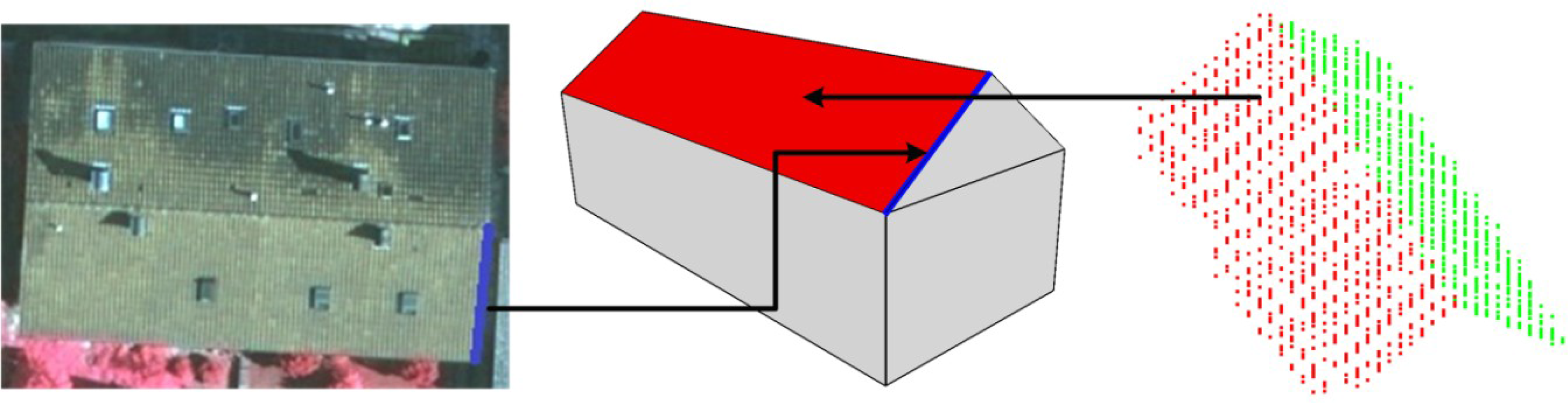
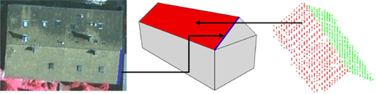
We analyzed how LiDAR data and aerial imagery complement each other. A LiDAR point cloud has dense 3D points, but these points are irregularly distributed and do not have accurate information regarding the break-lines, such as building boundaries. On the contrary, buildings exhibit sharp and clear edges in the optical imagery, but it is difficult to obtain the dense 3D points on the building’s surface. To find a way to tightly integrate LiDAR data and the aerial imagery for 3D building reconstruction, the selected object must have both sharp edges and explicit surfaces. For example, primitives such as flat roofs, gable roofs, and hipped roofs can satisfy this requirement. Suitable primitives will “glue” LiDAR point cloud data and optical imagery, as shown in Figure 1. In a primitive, the boundary information from the image (shown as the blue line) and the surface information from the point cloud (shown as the red plane) can be obtained. Thus far, the 3D building reconstruction problem can be solved as a primitive’s parameter estimation problem by optimizing a cost function formed by constraints from both LiDAR data and aerial imagery.
Additionally, from the computation point of view, primitive-based representation of a 3D building model has fewer parameters. For instance, to represent a flat roof, three parameters (width, length, and height) are used to represent the shape. Together with three parameters for position and three parameters for orientation, a total of nine parameters are sufficient to determine the shape and to locate the flat roof in 3D space. Thus, the solution can be computed easily and robustly.
2.2. Representation of Primitives
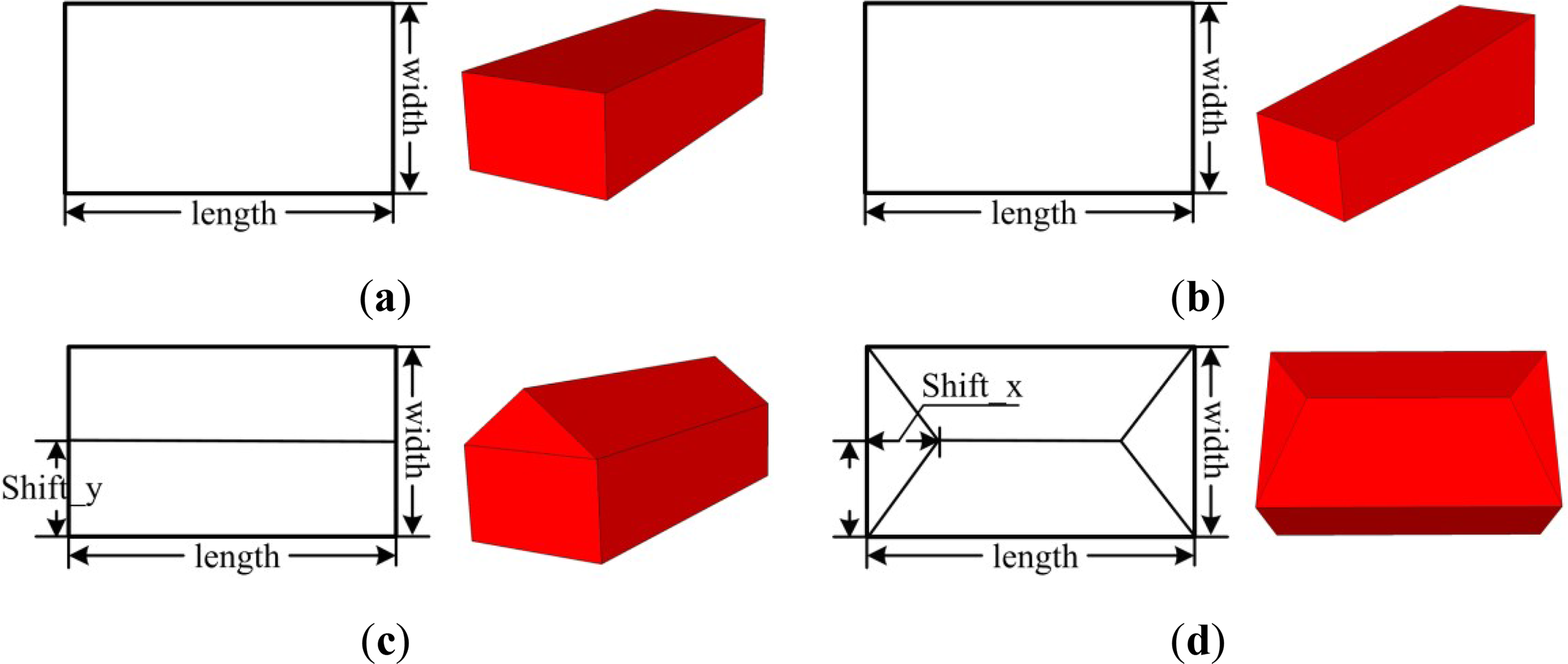
In theory, any primitive that has corresponding features in both a LiDAR point cloud (plane, curved surface, etc.) and an aerial imagery (corner, edge, etc.) can be used by the proposed modeling method. Non-symmetric and non-rectangular buildings can be represented by appending additional parameters to a simple symmetric primitive or constructing a new suitable primitive. Complex aggregated buildings can be decomposed and represented by a combination of single primitives. Some simple primitives are studied in this research and presented in Figure 2.
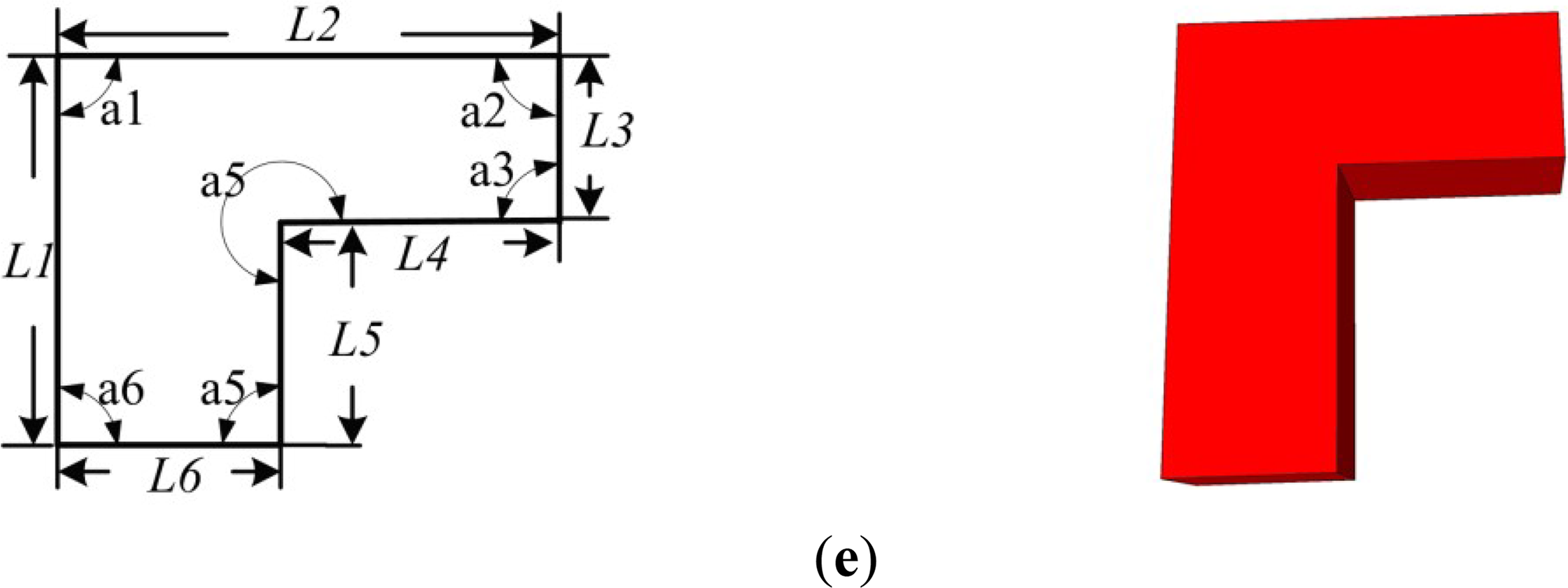
For each primitive in the library, it is sufficient to use three translation parameters (x, y, z) to represent the position and three rotation parameters (φ, ω, κ) to represent the rotation of the primitive relative to the global coordinate system, these parameters are defined as pose parameters. Moreover, the shape and size of the primitive can be described by the shape parameters, which can be seen in Figure 2. For example, a flat roof primitive has three shape parameters: width, length, and height. For a gabled roof, there will be an additional parameter—height of the roof ridge. Figure 3 illustrates the shape parameters that define a hipped roof primitive. In this research, we also define a variant of the flat roof as a complex roof primitive, which has a polygonal shape. An example of this complex flat roof primitive can be seen from Figure 2e. In this case, we use lengths (L1,L2,⋯⋯) and interior angles of the polygon (α1,α2,⋯⋯) to define the shape parameters of the complex roof with one planar surface having more than four edges.
2.3. Construction of Constraint Function
The main idea of this modeling method is to represent buildings by geometric primitives and construct a cost function using information from both LiDAR data and the aerial imagery, and then the pose parameters and shape parameters can be derived by minimizing the cost function.
This study uses a simple case to describe the construction of the cost function. A plane is chosen as a feature from LiDAR data, and a corner is selected as a feature from the aerial imagery. When a 3D building model has the correct shape and is located in the correct place in 3D space, two constraints must be satisfied. First, the back-projections of the primitive’s vertices onto the aerial image should be perfectly located on the corresponding corners; this constraint can be expressed by the co-linearity equation. Second, the primitive’s vertices should be exactly on the planes extracted from the LiDAR points; this constraint can be expressed by the point-to-plane distance. According to the two aforementioned constraints, three constraint functions can be established as Equation (1):
xi, yi: Projected image coordinates of the primitive’s vertex i;
xp, yp, f: Image coordinates of principle point and principle distance;
di: The distance of a primitive’s vertex i to the corresponding 3D roof plane;
: The elements of the rotation matrix that depend on the rotation angles;
X_i = [Xi Yi Zi]T: Coordinates of primitive’s vertex i in the object coordinate system;
X_S = [XS YS ZS]T: The object coordinates of the perspective center;
A, B, C, D: 3D Plane parameters that can be estimated from the 3D points located on the roof surface, and n = [A B C].
For example, the unknown parameters of a symmetrical gabled roof primitive are pose parameters (Xm, Ym, Zm, ωm, φm, κm) and shape parameters (l, w, h). l and w refer to the length and width of the gabled roof, h refers to the height of the roof ridge relative to Zm. Using shape parameters, we can derive vertex’s coordinate (Ui, Vi, Wi) of each primitive in the building model coordinate system. When transforming the primitive to the object coordinate system, three translate parameters (Xm, Ym, Zm) and three rotation parameters (ωm, φm, κm) are used, which can be expressed as Equation (2).
(Xi, Yi, Zi) can be transformed to the image coordinate using the co-linearity equation with the EOP (Exterior Orientation Parameters) and IOP (Interior Orientation Parameters) of the aerial image, the aforementioned transform process can be expressed as Equation (3):
In summary, the constraints for a symmetrical gabled roof primitive can be formulated as:
Using these constraints equations, the cost function can be constructed, which will be described in the following section.
2.4. Formulation of the Optimization Problem
In this study, 3D building reconstruction is considered as a primitive’s parameter optimization problem that includes variables and constraint functions, which can be seen from Equation (5). The variables considered in this research can be categorized into two groups: pose parameters (Xm, Ym, Zm, ωm, φm, κm) and shape parameters (l, w, h), which were defined in the previous section. The cost function is a quantified performance criterion, which evaluates the closeness of not only the LiDAR data but also the imagery data to the corresponding model. The cost function to be minimized can be formulated as Equation (6).
In Equation (6), F(sp, pp) is the cost function to be minimized, where sp represents the shape parameters of the primitive and pp represents the pose parameters relative to the global coordinate system; (xi, yi) is the image coordinates of primitive’s vertex i, which can be derived by corner extraction from aerial imagery; (x′i, y′i) is the back projected image coordinates of primitive’s vertex i, which can be calculated by the co-linearity equation; di is the distance of a primitive’s vertex i to the corresponding roof surface; wxi, wyi, and wdi are the weight values, which are determined by the estimated errors of the observations. In this study, wxi and wyi are set to one pixel and wdi is set to 0.005 m according to the estimated errors, which will be discussed in Section 4.2.
The Equation (6) is a non-linear function between the unknown parameters and observations. To minimize the cost function, it should be transformed to a linear form using Taylor series expansion, which can be written as Equation (7):
In Equation (7), xi, yi are the projected image coordinates of the primitive’s vertex i ; (Xm0, Ym0, Zm0, ωm0, φm0, κm0, l0, w0, h0) are the initial values of the unknown parameters; A is the Jacobian matrix about the unknown parameters; exi, eyi, edi are the errors introduced by omitting items with high order derivatives. Applying the least square method together with the Newton’s iterative approach, the increments of unknown parameters ξ can be solved as in Equation (8).
where,
P: The weight matrix;
ξ: The increments of Xm, Ym, Zm, ωm, φm, κm, l, w, h.
The iterative process is stopped when the increments of unknown parameters are smaller than predefined limits, and then the optimal model parameters are derived. Finally, the 3D building roof can be represented by these primitives with the optimized parameters.
2.5. Workflow to Integrate the Proposed Modeling Method into a Building Reconstruction Framework
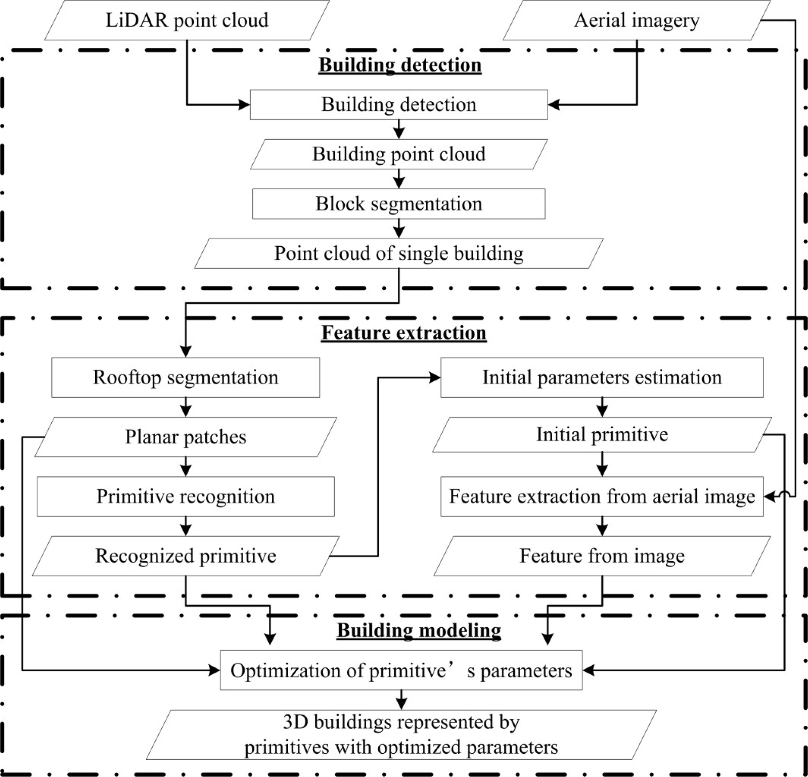
In this paper, we are focusing on the proposed building modeling method, by integrating LiDAR data and aerial imagery. To integrate the proposed modeling method into a complete building reconstruction framework, we applied some automatic building detection and feature extraction algorithm to derive the necessary input for the building modeling. The detailed data processing procedure is described in Section 3.2.2. Figure 4 shows the flowchart of this primitive-based building reconstruction framework. It consists of three stages: (1) Building detection. This step combines the LiDAR point cloud and aerial imagery for building detection and individual building segmentation. The 3D points of each single building can be extracted at this stage. (2) Feature extraction. In this process, rooftop planar patches are extracted from LiDAR point cloud and the building corners are extracted from the aerial imagery. These features are the key inputs of the primitive optimization. (3) Building roof modeling. This is a primitive parameters optimization step. All of the features extracted in step 2 are utilized for the optimization process. Using a non-linear least square optimization method, the optimized primitives’ parameters are computed. Finally, the 3D building roof models are represented with the optimized parameters.
3. Experimental Results
To evaluate the reconstruction accuracy of the proposed method, a simulation experiment and a real data experiment utilizing a data set provided by ISPRS (International Society for Photogrammetry and Remote Sensing) were conducted, which will be described in detail in the following sections.
3.1. Simulation Experiment
The aim of the controlled simulation experiment is to study the building modeling accuracy of the proposed modeling method by comparing to the photogrammetric means. And the result of the simulation experiment will also provide the basis of selecting images. How many images should be used, and what the accuracy will reach? If one image is used, which one is better (nadir image or oblique image)?
In the simulation experiment, one gabled roof was adopted as the test primitive. And then the building roof’s point cloud and two images were generated. The point density of the simulated point cloud was 4 points/m2, and the ground resolution of the digital aerial images was approximately 8 cm. Different methods were utilized to reconstruct the building’s model, and 3D coordinates of the building’s corners (a gabled roof has 6 corners) were calculated. The calculated corners were compared with the true values (because the building is simulated, the correct 3D coordinates of corners are known), and then the horizontal accuracy and the vertical accuracy were evaluated. The simulation experiments were conducted using three separate schemes which will be described as following.
3.1.1. Space Intersection Method vs. the Proposed Modeling Method
In the first simulation experiment, a building roof's point cloud and two images were generated. Using the stereo image pair, 3D coordinates of the roof's corners can be calculated by the space intersection method. Using the proposed modeling method, 3D coordinates of the roof's corners can also be calculated. These two types of calculated corners will be compared with the true values, and then the horizontal and vertical accuracy can be evaluated. All simulated data were error free except for the 2D corner image coordinates. Different levels of errors (from 0 to 5 pixels) were added to generate 2D corner image coordinates with errors. Thus, we can observe how the space intersection method and the proposed method were influenced by these errors.
For each level of error, the test primitive was repeatedly processed 100 times (it equaled to compute a statistical result of 6 × 100 = 600 corners). The root mean square error (RMSE) of the gabled roof was calculated (comparing the calculated value with the true value). The result is presented in Figure 5.
It can be seen that:
The vertical accuracy of the proposed modeling method is much better than the space intersection method. This is anticipated because our method utilized the information from LiDAR data, and as we know, LiDAR often has better vertical accuracy than space intersection of images.
The horizontal accuracy of the proposed method is also slightly better than space intersection method. The possible explanation is that our method constrains the reconstructed object point in the extracted features (e.g., plane) from the LiDAR point cloud, whereas the object point calculated by space intersection method does not have this constraint.
The difference of accuracy becomes more and more notable with increasing level of error in the 2D corner image coordinates. The proposed method is more robust against this type of error.
3.1.2. Nadir Aerial Image vs. Oblique Aerial Image
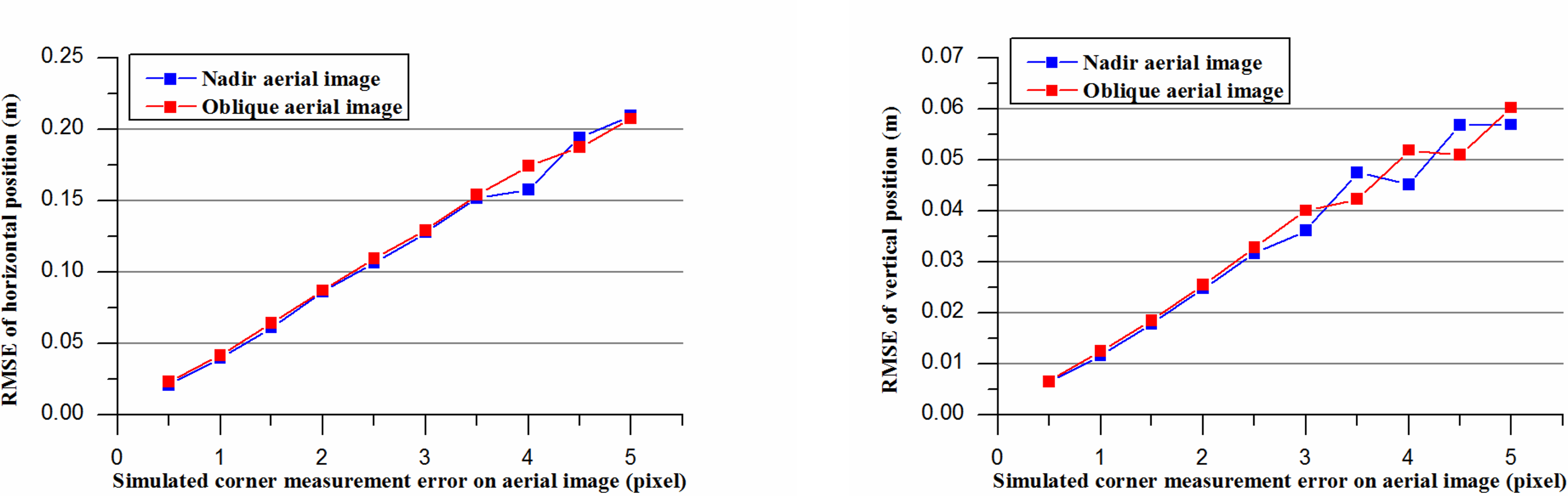
In the second simulation experiment, the nadir aerial image and the oblique aerial image were utilized to find which one can derive the better reconstruction result together with the LiDAR point cloud using the proposed modeling method. In the simulation process, different levels of errors (from 0 to 5 pixels) were also added to generate 2D corner image coordinates with errors. The results were presented in Figure 6. It can be seen that almost the same reconstruction results were derived whether using nadir aerial image or oblique aerial image, so the shooting angle of the aerial image was not important to the reconstruction result. This simulation experiment is meaningful because most of the current LiDAR systems are equipped with aerial camera, which can easily derive the nadir aerial image.
3.1.3. One Aerial Image vs. Two Aerial Images
In the third simulation experiment, one aerial image and two aerial images were used respectively in the proposed optimization procedure, and the results were compared.
From Figure 7, it can be seen that the horizontal accuracy and the vertical accuracy were slightly better when using two aerial images. This can be explained that more constraints were added in the optimization procedure. It is noted that one aerial image is sufficient for the proposed modeling method to generate accurate building models. When two or more overlapping images are available, the accuracy can be further improved.
3.2. Real Data Experiment
In addition to the simulation experiment, a practical experiment using the data set provided by ISPRS was also performed to verify the geometric accuracy of the proposed method.
3.2.1. Description of the Data Set
Using the data set provided by ISPRS (International Society for Photogrammetry and Remote Sensing), a real data experiment was carried out to verify the applicability and the geometric accuracy of the proposed method. The test data set contains Airborne Laser Scanner (ALS) data and digital CIR images that were available at the ISPRS web site. The ALS data was acquired on 21 August, 2008, via a Leica ALS50 system, where the average flying height is 500 m that is approximately a point density of 4 points/m2. The digital CIR aerial images were acquired from an Intergraph/ZI DMC (Digital Mapping Camera) on 24 July 2008, with an 8 cm ground resolution, where the orientation parameters are distributed together with the images in the level of pixel geo-referencing accuracy [36].
The test data was captured over Vaihingen in Germany, where they came from three test areas. For each test area, the reference data of various object classes are available to this project. In this study, the test area 3 “Residential Area” was selected for the experiments to validate the geometric accuracy of the proposed method. It is a residential area with small, detached houses. Most of the buildings in this area can be represented by the gabled roof primitive. Figure 8 shows the digital imagery and the corresponding LiDAR point cloud of the test area.
3.2.2. Description of Data Processing
As can be seen from Figure 4, there are three steps to incorporate the modeling method into a building reconstruction framework, these are: building detection, feature extraction, and building modeling (primitive parameters optimization). The test area was processed by this building reconstruction procedure.
Building Detection and Segmentation
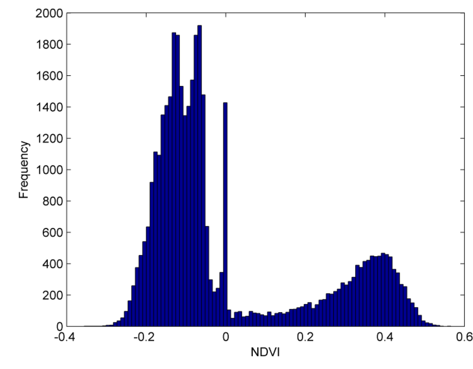
In order to derive 3D building models, building regions must be detected and extracted from the LiDAR data first. The original point cloud is used in this study instead of the re-sampled grid data. The building detection procedure consists of three main steps. First, ground points are separated from non-ground points by a filter method proposed by Axelsson [37], then the high rise points can be identified using a specified height threshold above the ground. In this study, a threshold of 2 m is adopted because most of buildings in the test area are taller than 2 m. The high-rise points derived in this step mainly contain building points and tree points. In the second step, buildings points are separated from tree points by using NDVI (Normalized Difference Vegetation Index) derived from the aerial CIR imagery. Every high-rise point is projected back on the aerial imagery to derive the corresponding pixel location, and then NDVI of each high-rise point is calculated using near IR (Infrared) and R (Red) values by Equation (9):
When NDVI of each high rise point is calculated, most of the tree points can be removed based on a NDVI threshold (0.1 in this area) that is determined by histogram analysis, as can be seen from Figure 9. In the final step, the remaining points are segmented into clusters using Euclidean clustering method introduced by Rusu [38], and then two rules will be used to identify the tree clusters that could not be removed by using NDVI. One is that tree clusters often have smaller area; the other is that points in the tree clusters often have multiple echoes, so the ratio of multiple echo points will help to remove the tree clusters. Figure 10a shows the final result of building detection. It can be seen that the ground points and tree points are removed, and the blue points superimposed on the aerial image are the points belong to buildings. The results of building blocks segmentation are presented in Figure 10b, where different colors indicate different buildings. As can be seen, most buildings are segmented correctly. If the buildings are very close to each other and have similar height, the automatic segmentation cannot work. In that case, the human-interactive operation is needed to obtain the correct results.
After the building detection, each building’s point cloud is clustered as an individual point set, then the building models can be reconstructed one by one using these point sets. Before the proposed optimization method is used to reconstruct the building models, relevant features should be extracted from LiDAR data and aerial imagery. The extraction process is described as follows.
Rooftop Planar Patches Extraction and Primitive Recognition
Rooftop planar patches are essential input of the proposed modeling method. The planar patches of each individual building point cloud must be extracted. This is a segmentation procedure. According to Tarsha-kurdi et al. [11], RANSAC algorithm is an efficient segmentation algorithm in terms of processing time and sensitivity to point cloud characteristics. So, a robust plane fitting algorithm based on RANSAC [39] is adopted to extract planar patches of each individual rooftops in this study. As a result of RANSAC plane extraction, each individual building point set can be segmented into different clusters and each cluster actually describes a 3D plane. Figure 10c shows the result of building rooftops segmentation, different colors indicate different roof planar patches of each building.
When the rooftop planar patches are segmented, the type of the roof primitive can be recognized according to the number of planes and the relationship between them. In the test area, there are some simple building primitives, which are illustrated in the Section 2.2, thus, we use the number of 3D planes extracted from the LiDAR point cloud for the primitive selection. If one plane is extracted from the point cloud, then it will be a flat roof or a shed roof; if there are two planes, it is a gabled roof. In the presence of three and four planes that correspond to a gabled roof with one dormer and a gabled roof with two dormers, respectively. When the type of the building primitive has been determined, the initial primitive parameters can be estimated from the 3D planes extracted from the LiDAR points that can be used for the optimization procedure.
Corner Extraction from the Aerial Image
After rooftop segmentation, the LiDAR points located on the same plane can be extracted and the edge pixels and corners of each building can be detected with the help of each planar patch using the following steps. First, the 3D boundary points of each planar patch were obtained by using the modified convex hull method [40], and then these 3D boundary points were grouped into different groups by using sleeve algorithm [29]. They are presented in Figure 11a,b. Second, the grouped 3D boundary points were projected back to the aerial imagery and the canny detector [41] was applied to the aerial imagery to derive the 2D edge points. A buffer (15 pixels, indicates approximately two times of the point spacing in LiDAR point cloud) surrounding these projected boundary points was defined to find the corresponding 2D edge points on the image. These are demonstrated in Figure 11c and Figure 11d. Finally, the RANSAC algorithm [42] was applied in each 2D edge pixels group to filter the non-edge pixels and derive straight lines (Figure 11e). The 2D corners can be extracted by the intersection of the neighbor straight lines and they are shown Figure 11f. In practice, some real corners in aerial imagery cannot be extracted automatically due to the occlusions or poor contrast, especially in smaller buildings. In this case, the corners on the image will be extracted manually.
Optimization of the Primitive’s Parameters
When planar patches from the LiDAR data and corners from the aerial images have been extracted, as mentioned in Section 2.4, a cost function can be constructed and a non-linear least squares optimization is performed to obtain the optimal primitive parameters. Therefore, the 3D rooftop can be represented by primitives with optimized parameters. After modeling the roofs, the terrain elevations are used to determine the building base height and the final 3D building model can be derived by extruding the roof models to the building base height.
3.2.3. Real Data Experimental Result
To validate the geometric accuracy of the proposed method, the reconstruction results are evaluated by ISPRS reference data. The requirement of the submitted data to the ISPRS Test Project is DXF (Drawing Exchange Format) files, which contain closed 3D polygons that correspond to the outlines of the reconstructed roof planes in the object coordinate system. The examples presented in Figure 12 are the building roofs in DXF files.
The organizer of this ISPRS Test Project maintains the web page that show the continuous comparison result of different methods [43], and the detailed results of this ISPRS benchmark on urban object detection and 3D reconstruction can be referred to Rottensteiner et al. [44]. The geometric accuracy comparison result of the 3D building reconstruction of test Area 3 is presented in Table 1. The result of the proposed method is highlighted in green. In this table, different research institutions who submit their reconstruction result in this test area are listed, and the horizontal accuracy (RMS) and vertical accuracy (RMSZ) of the geometrical errors of the reconstruction are also listed. RMS refers to average root mean square error in XY plane and RMSZ refers to average root mean square error in Z direction.
In Table 1, it can be noted that the proposed method achieves a higher geometric accuracy on both of the plane and elevation accuracy. It is because the corner points of an optimized primitive must satisfy the constraints of a 3D plane in LiDAR data and the pixel coordinates in the aerial image at the same time. As a result, the advantages of the two complementary data sets are effectively integrated for building reconstruction purpose.
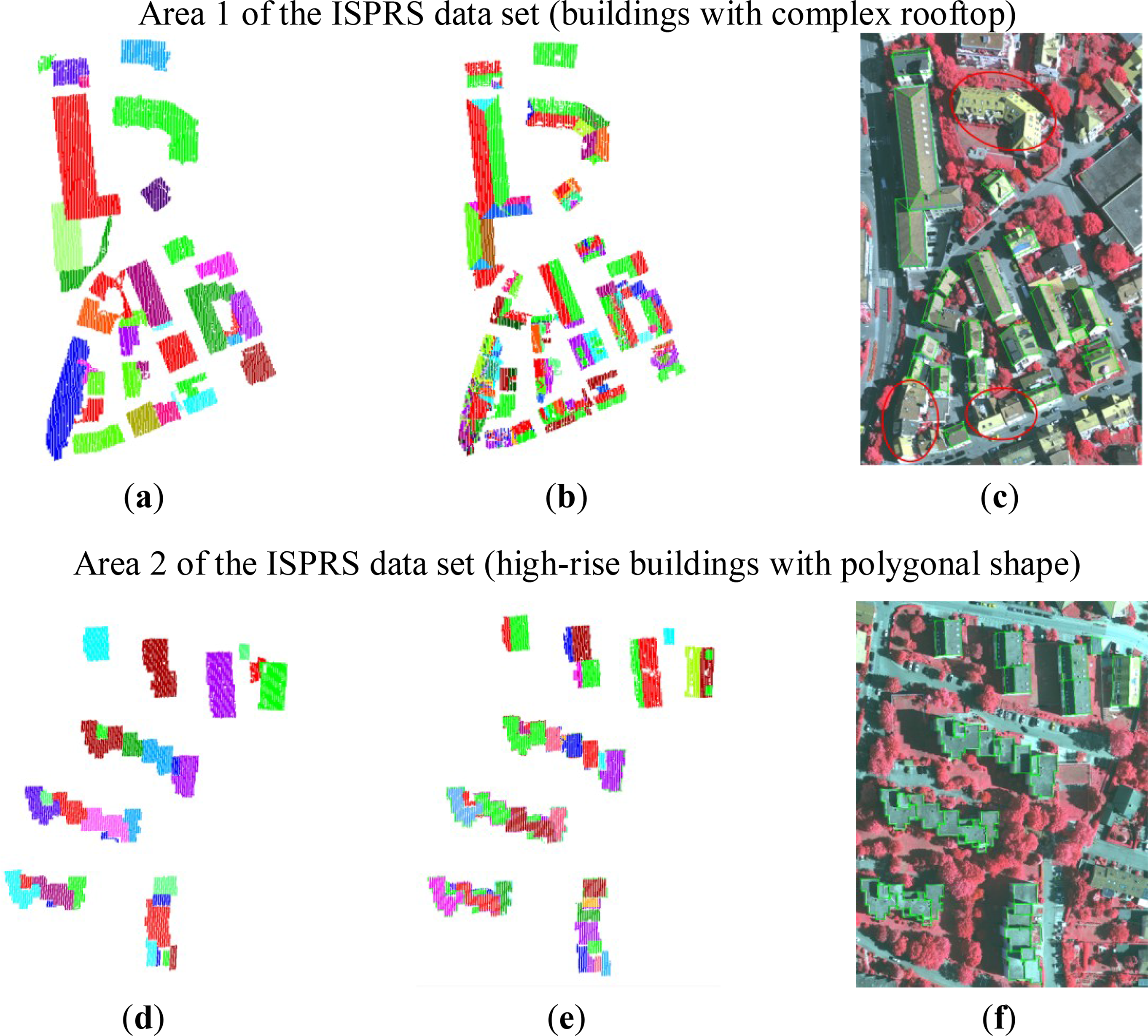
In order to further validate the feasibility of the proposed method, we have applied our modeling method to the other data sets of the ISPRS benchmark (Area 1 and Area 2). The results can be seen from Figure 13. Area 1 is characterized by complex rooftops, and Area 2 is characterized by asymmetrical gabled roofs and complex flat roofs. The asymmetrical gabled roof primitive is defined for the asymmetrical gabled roof’s generation and complex flat roof primitive (Figure 2e) is defined for the generation of the flat roof with a polygonal shape. As can be seen from Figure 13, some complex buildings with many dormers or having the shape of the combination of basic primitives cannot be properly reconstructed in Area1 (in red circle) at current stage.
4. Discussions
4.1. The Variant Primitive and Primitive Recognition
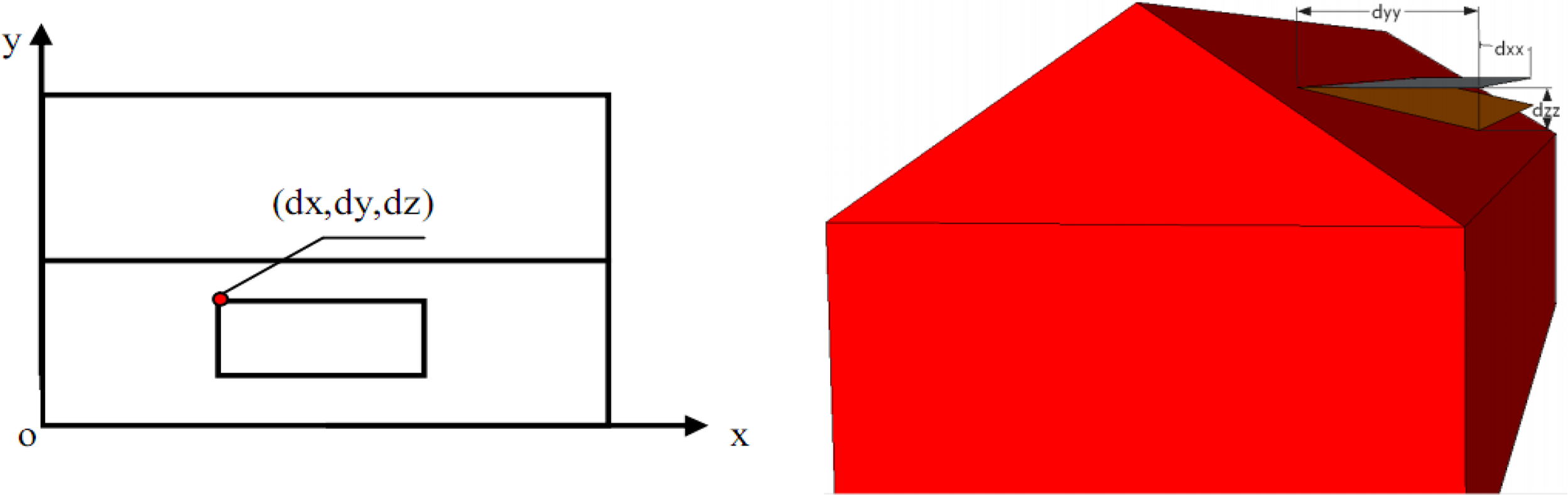
As presented in Figure 8a, there are some gabled roofs with dormers in the test area. In order to reconstruct these buildings, the variant primitives were introduced with gabled roofs attached in one or two dormers. Figure 14 shows a gabled roof with one dormer, in this case, additional six parameters are used to append a dormer to the gabled roof primitive, where three parameters (dx, dy, dz) for the relative position to the original point of the gabled roof and the other three parameters (dxx, dyy, dzz) for the shape of the dormer. Using the variant primitive, the proposed method can generate a building model with details.
In this study, only primitives with rectangular shape are used and the type of roof primitive was determined by the number of planes extracted from LiDAR. Apparently, neither non-rectangular buildings nor complex aggregated buildings can be recognized by this simple strategy. Thus, the suggested future work can focus on automatic recognition and selection of the most optimal primitive in a library or complex building decomposition.
4.2. Weight Values of the Cost Function
In the proposed method, there are two different kinds of constraints in the cost function. Two different weight values are assigned to those two constraints. The first constraint is the back-projections of the primitive’s vertices to the aerial image (x′i, y′i). It should be perfectly located on the corresponding extracted corners (xi, yi). wxi is the weight value of (x′i − x′i) and wyi is the weight value of (y′i − y′i), which are determined by the estimated errors. When the first constraint is satisfied, (x′i − x′i) and (y′i − y′i) should be very small, thus, wxi and wyi should be small too. In this research, wxi and wyi are set to one pixel.
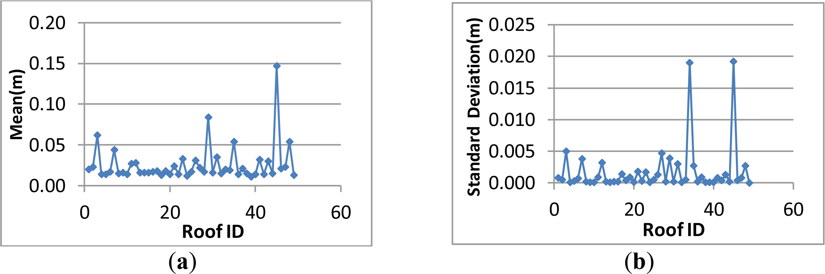
The second constraint is that the primitive’s vertices should be exactly on the planes extracted from the LiDAR points. In this research, each 3D plane is derived from LiDAR points that belong to the same roof surface and di is the distance of a primitive vertex i to the corresponding 3D plane. The weight of di(wdi) can be determined by the plane fitting result. wdi is set to 0.005 m in this paper based on histogram analysis [50]. They are presented in Figure 15.
4.3. Sensitivity to the Initial Parameters Using the Proposed Method
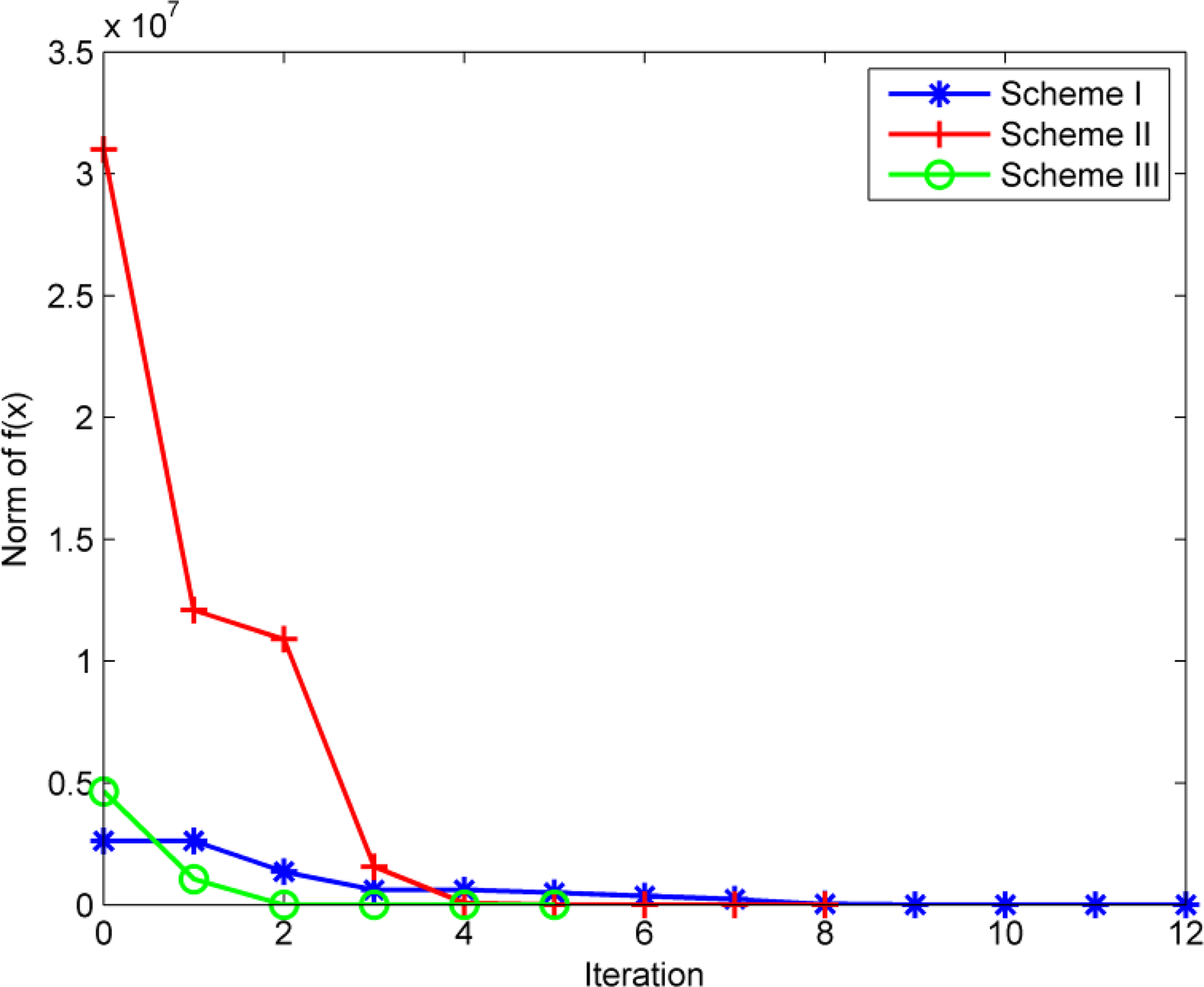
One advantage of the proposed method is that the optimization processes is not sensitive to the initial shape and pose parameters. A gabled roof in the test area is used to show this fact: three groups of initial shape and pose parameters are used for the optimization of the gabled roof parameters which can be seen in Table 2. As mentioned in Section 2.3, there are six pose parameters (Xm, Ym, Zm, ωm, φm, κm) and three shape parameters (l, w, h) to be optimized for a gabled roof. In this experiment, the initial values of (Xm, Ym, Zm) are set to the center of the LiDAR point cloud belong to the experimental gabled roof, and the initial values of (ωm, φm) are set to zero. So, only κm (the orientation of the building) and (l, w, h) are listed in Table 2. The optimization is performed by using different initial values in Table 2. The wireframes of both initial models and optimized models are back-projected to the image, which are shown in Figure 16 (blue wireframes are back-projections of initial models and green wireframes are back-projections of optimized models). It can be seen that the initial models obviously deviate from the true shape and place, and they can be corrected to fit in a real building well after the optimization process. This can also be verified by Figure 17. The optimization can quickly converge to a stable solution in three schemes. The efficiency of the proposed method is also can be seen from Figure 17. For the test gabled roof, the minimum number of iterations is five and the maximum number of iterations is twelve according to different initial model values. Thus, the proposed algorithm has a high efficiency in the optimization procedure. The final optimization results can also be seen in Table 2, the optimization values of the model parameters are almost the same as those in three schemes. It can be concluded that in the proposed method, the cost function constructed by the constraints from both LiDAR and images has a wide region of convergence.
4.4. Accuracy Assessment
As shown in Table 1, among methods that were evaluated by the ISPRS Test Project for the building roof reconstruction [44], our building modeling method is the only method that uses both aerial image and LiDAR point cloud, and the only method that is primitive-based. The average root mean square error in XY plane is 0.6 m, and the error in Z direction is 0.1 m in our modeling result, which indicates that the proposed building modeling method achieves a higher geometric accuracy on both of the plane and elevation accuracy. The organizer of this ISPRS Test Project also provided some images that visualize the evaluation results, which can be seen from Figure 18. Figure 18a shows the difference between two DSMs (Digital Surface Model) that were derived from the roof planes of the result and the reference. The difference is evaluated on pixels where a plane was found in both data sets; all other pixels are displayed in white. Figure 18b shows the evaluation of building reconstruction on a per-pixel level. In this figure, yellow means correct roofs, blue means missed roofs, and red areas are part of the background but were reconstructed as roofs by mistake.
There are some factors that will lead to the errors in the reconstructed building model. For example, the density of the point cloud and the quality of the building roof point cloud detection and segmentation. Aerial image is used in the proposed building modeling method, so the accuracy of the interior and exterior orientation parameters and the accuracy of feature detection will also influence the building reconstruction result. Furthermore, the proposed building modeling method is a model driven method; additional building reconstruction errors will be introduced because of the difference between real building and the model. For example, some detailed features of buildings cannot be reconstructed when buildings do not strictly coincide with primitives. In Figure 18a, there are some small blue dots on the roofs, these are chimneys on the rooftops. They are missed due to their small areas. In addition, some missed parts of roofs (in blue) and some false parts of roofs (in red) can be observed in Figure 18b. The difference between real buildings and primitives may lead to a decrease in geometrical accuracy. In Figure 18b, the building in the red rectangle and its corresponding image illustrates this situation.
5. Conclusions and Future Work
LiDAR data and aerial imagery has unique advantages and disadvantages for building reconstruction. To combine the strengths of these two data sources for the generation of building roof models, a primitive-based 3D building roof modeling method is proposed in this study. The main idea is to represent building roofs by parametric primitives and construct cost functions using information from both LiDAR data and the aerial imagery, thus that the 3D building reconstruction problem is converted to a primitive’s parameter optimization problem. From the controlled simulation experiments, it can be seen that the proposed modeling method has a higher vertical accuracy comparing to the traditional photogrammetry method. The real data experimental results demonstrate that the proposed reconstruction method can tightly integrate LiDAR data and the aerial imagery, and it can generate 3D building models with the average root mean square error of 0.6 m in XY plane and 0.1 m in Z direction in the study case.
In general, experimental results show that the proposed method can tightly integrate LiDAR data and the aerial imagery to generate more accurate building roof models. Another strength of the proposed modeling method is that it can reconstruct building roof models using LiDAR data and single nadir aerial imagery, which makes it is more applicable to the current LiDAR systems equipped with an aerial camera. Furthermore, the experimental results also show that by adding a component, such as dormer, a variant of the simple primitive is constructed and the proposed modeling method can generate a building model with some details. Comparing to the existing two-step method, where LiDAR data and optical imagery are used in a sequential process, the proposed modeling method is a one-step method. It means when optimizing the parameters of a building model, constraints from both LiDAR data and imagery are working simultaneously, and both of these constraints affect the model parameters during the optimization procedure.
The limitation of the proposed method is that it is a model driven method, so the differences between the real buildings and the primitives will lead to a decrease in geometrical accuracy. Therefore, the future research will focus on more building primitives and the complex building decomposition, so that the improved building models can more closely represent the real buildings. In addition, the proposed modeling method is based on 3D primitives and parameters optimization; it offers the possibility of simultaneously processing both the aerial data and the ground data, such as mobile LiDAR point cloud. Thus, future work will fuse more data sets to generate more complete models of complex buildings.
Acknowledgments
This work is supported by National Natural Science Foundation of China Grant No. 41171265 and 40801131, and the National Basic Research Program of China (973 Program) Grant No. 2013CB733402. This work is also funded by the project for free exploration of State Key Laboratory of Remote Sensing Science Grant No. 14ZY-04 and open foundation of Guangxi Key Laboratory of Spatial Information and Geomatics Grant No. 1103108-04.
The author would like to acknowledge the provision of the Vaihingen data set by the German Society for Photogrammetry, Remote Sensing and Geoinformation [51].
Author Contributions
Wuming Zhang proposed this primitive-based modeling method and guided the research work related to this method. Hongtao Wang did research on the building detection from LiDAR point cloud and the aerial imagery and modeling experiment. Yiming Chen did research on the segmentation of buildings and roofs. Kai Yan did research on features extraction from LiDAR point cloud and the aerial imagery. Mei Chen evaluated the proposed modeling method using real data set.
Conflicts of Interest
The authors declare no conflict of interest.
References
- Sohn, G.; Jung, J.; Jwa, Y.; Armenakis, C. Sequential modeling of building rooftops by integrating airborne LiDAR data and optical imagery: Preliminary results. Proceedings of VCM 2013—The ISPRS Workshop on 3D Virtual City Modeling, Regina, Cannada, 28 May 2013; pp. 27–33.
- Mayer, H. Automatic object extraction from aerial imagery—A survey focusing on buildings. Comput. Vis. Image Underst 1999, 74, 138–149. [Google Scholar]
- Remondino, F.; El-Hakim, S. Image-based 3D modelling: A review. Photogramm. Rec 2006, 21, 269–291. [Google Scholar]
- Debevec, P.E.; Taylor, C.J.; Malik, J. Modeling and rendering architecture from photographs: A hybrid geometry-and image-based approach. Proceedings of the 23rd Annual Conference on Computer Graphics and Interactive Techniques, New Orleans, LA, USA, 4–9 August 1996; pp. 11–20.
- Wang, R.; Ferrie, F.P. Camera localization and building reconstruction from single monocular images. In Proceedings of the 2008. IEEE Computer Society Conference on Computer Vision and Pattern Recognition Workshops, Anchorage, AK, USA, 23–28 June 2008; pp. 1–8.
- Hammoudi, K.; Dornaika, F. A featureless approach to 3D polyhedral building modeling from aerial images. Sensors 2011, 11, 228–259. [Google Scholar]
- Zebedin, L.; Klaus, A.; Gruber-Geymayer, B.; Karner, K. Towards 3D map generation from digital aerial images. ISPRS J. Photogramm. Remote Sens 2006, 60, 413–427. [Google Scholar]
- Bulatov, D.; Rottensteiner, F.; Schulz, K. Context-based urban terrain reconstruction from images and videos. Proceedings of the XXII ISPRS Congress of the International Society for Photogrammetry and Remote Sensing ISPRS Annals, Melbourne, Australia, 25 August–1 September 2012; p. 3.
- Brenner, C. Building reconstruction from images and laser scanning. Int. J. Appl. Earth Obs. Geoinf 2005, 6, 187–198. [Google Scholar]
- Haala, N.; Kada, M. An update on automatic 3D building reconstruction. ISPRS J. Photogramm. Remote Sens 2010, 65, 570–580. [Google Scholar]
- Tarsha-Kurdi, F.; Landes, T.; Grussenmeyer, P. Extended RANSAC algorithm for automatic detection of building roof planes from LiDAR data. Photogramm. J. Finl 2008, 21, 97–109. [Google Scholar]
- Vosselman, G. Building reconstruction using planar faces in very high density height data. Int. Arch. Photogramm. Remote Sens 1999, 32, 87–94. [Google Scholar]
- Awrangjeb, M.; Fraser, C.S. Automatic segmentation of raw LiDAR data for extraction of building roofs. Remote Sens 2014, 6, 3716–3751. [Google Scholar]
- Awrangjeb, M.; Zhang, C.S.; Fraser, C.S. Automatic extraction of building roofs using LiDAR data and multispectral imagery. ISPRS J. Photogramm. Remote Sens 2013, 83, 1–18. [Google Scholar]
- Rottensteiner, F. Roof plane segmentation by combining multiple images and point clouds. Proceedings of the Photogrammetric Computer Vision and Image Analysis Conference, Saint-Mandé, France, 1–3 September 2010; pp. 245–250.
- Dorninger, P.; Pfeifer, N. A comprehensive automated 3D approach for building extraction, reconstruction, and regularization from airborne laser scanning point clouds. Sensors 2008, 8, 7323–7343. [Google Scholar]
- Sampath, A.; Shan, J. Segmentation and reconstruction of polyhedral building roofs from aerial lidar point clouds. IEEE Trans. Geosci. Remote Sens 2010, 48, 1554–1567. [Google Scholar]
- Zhou, Q.-Y.; Neumann, U. 2.5D building modeling by discovering global regularities. Proceedings of the 2012 IEEE Conference on Computer Vision and Pattern Recognition (CVPR), Providence, RI, USA, 16–21 June 2012; pp. 326–333.
- Haala, N.; Brenner, C.; Anders, K.-H. 3D urban GIS from laser altimeter and 2D map data. Int. Arch. Photogramm. Remote Sens 1998, 32, 339–346. [Google Scholar]
- Henn, A.; Groger, G.; Stroh, V.; Plumer, L. Model driven reconstruction of roofs from sparse LiDAR point clouds. ISPRS J. Photogramm. Remote Sens 2013, 76, 17–29. [Google Scholar]
- Kada, M.; McKinley, L. 3D building reconstruction from LiDAR based on a cell decomposition approach. Int. Arch. Photogramm. Remote Sens. Spat. Inf. Sci 2009, 38, W4. [Google Scholar]
- Suveg, D.; Vosselman, G. Reconstruction of 3D building models from aerial images and maps. ISPRS J. Photogramm. Remote Sens 2004, 58, 202–224. [Google Scholar]
- Lafarge, F.; Descombes, X.; Zerubia, J.; Pierrot-Deseilligny, M. Structural approach for building reconstruction from a single DSM. IEEE Trans. Pattern Anal. Mach. Intell 2008, 32, 135–147. [Google Scholar]
- Chen, L.C.; Teo, T.A.; Hsieh, C.H.; Rau, J.Y. Reconstruction of building models with curvilinear boundaries from laser scanner and aerial imagery. Proceedings of the Advances in Image and Video Technology, Taiwan, China, 10–13 December 2006; Chang, L.W., Lie, W.N., Eds.; 4319, pp. 24–33.
- Cheng, L.A.; Gong, J.Y.; Li, M.C.; Liu, Y.X. 3D building model reconstruction from multi-view aerial imagery and LiDAR data. Photogramm. Eng. Remote Sens 2011, 77, 125–139. [Google Scholar]
- Kim, C.J.; Habib, A. Object-based integration of photogrammetric and lidar data for automated generation of complex polyhedral building models. Sensors 2009, 9, 5679–5701. [Google Scholar]
- Sohn, G.; Dowman, I. Data fusion of high-resolution satellite imagery and LiDAR data for automatic building extraction. ISPRS J. Photogramm. Remote Sens 2007, 62, 43–63. [Google Scholar]
- Demir, N.; Baltsavias, E. Automated modeling of 3D building roofs using image and LiDAR data. Proceedings of the XXII Congress of the International Society for Photogrammetry, Remote Sensing, Melbourne, Australia, 25 August–1 September 2012.
- Ma, R. Building Model Reconstruction from LiDAR Data and Aerial Photographs., Ph.D. Thesis. The Ohio State University, Columbus, OH, USA, 2004.
- Rottensteiner, F.; Trinder, J.; Clode, S.; Kubik, K. Fusing airborne laser scanner data and aerial imagery for the automatic extraction of buildings in densely built-up areas. Int. Arch. Photogramm. Remote Sens. Spat. Inf. Sci 2004, 35, 512–517. [Google Scholar]
- Arefi, H.; Reinartz, P. Building reconstruction using DSM and orthorectified images. Remote Sens 2013, 5, 1681–1703. [Google Scholar]
- Kwak, E. Automatic 3D Building Model Generation by Integrating LiDAR and Aerial Images Using a Hybrid Approach. Ph.D. Thesis. University of Calgary, Calgary, AB, Canada, 2013. [Google Scholar]
- Seo, S. Model-Based Automatic Building Extraction from Lidar and Aerial Imagery., Ph.D. Thesis. The Ohio State University, Columbus, OH, USA, 2003.
- Wang, S.; Tseng, Y.-H.; Habib, A.F. Least-squares building model fitting using aerial photos and LiDAR data. Proceedings of the ASPRS 2010 Annual Conference, San Diego, CA, USA, 26–30 April 2010.
- Zhang, W.; Grussenmeyer, P.; Yan, G.; Mohamed, M. Primitive-based building reconstruction by integration of LiDAR data and optical imagery. Int. Arch. Photogramm. Remote Sens. Spat. Inf. Sci 2011, 38, 7–12. [Google Scholar]
- Rottensteiner, F.; Sohn, G.; Gerke, M.; Wegner, J.D. ISPRS Test Project on Urban Classification and 3D Building Reconstruction. Available online: http://www.itc.nl/ISPRS_WGIII4/docs/ComplexScenes.pdf (accessed on 7 Juanuary 2013).
- Axelsson, P. DEM generation from laser scanner data using adaptive TIN models. Int. Arch. Photogramm. Remote Sens 2000, 33, 111–118. [Google Scholar]
- Rusu, R.B. Semantic 3D object maps for everyday manipulation in human living environments. Künstl. Intell 2010, 24, 345–348. [Google Scholar]
- Schnabel, R.; Wahl, R.; Klein, R. Efficient ransac for point-cloud shape detection. In Computer Graphics Forum; Wiley Online Library: Hoboken, NJ, USA, 2007; Volume 26, pp. 214–226. [Google Scholar]
- Sampath, A.; Shan, J. Building boundary tracing and regularization from airborne LiDAR point clouds. Photogramm. Eng. Remote Sens 2007, 73, 805–812. [Google Scholar]
- Canny, J. A computational approach to edge detection. IEEE Trans. Pattern Anal. Mach. Intell 1986, 8, 679–698. [Google Scholar]
- Fischler, M.A.; Bolles, R.C. Random sample consensus: A paradigm for model fitting with applications to image analysis and automated cartography. Commun. ACM 1981, 24, 381–395. [Google Scholar]
- ISPRS Test Project on Urban Classification and 3D Building Reconstruction: Results. Available online: http://brian94.de/isprsIII_4_test_results/test_results_a3_recon.html (accessed on 7 August 2014).
- Rottensteiner, F.; Sohn, G.; Gerke, M.; Wegner, J.D.; Breitkopf, U.; Jung, J. Results of the ISPRS benchmark on urban object detection and 3D building reconstruction. ISPRS J. Photogramm. Remote Sens 2013, 93, 256–271. [Google Scholar]
- Rau, J.-Y. A line-based 3D roof modell reconstruction algorithm: TIN-merging and reshaping (TMR). Proceedings of the ISPRS Annals of the Photogrammetry, Remote Sensing and Spatial Information Sciences Conference, Melbourne, Australia, 25 August–1 September 2012; pp. 287–292.
- Elberink, S.O.; Vosselman, G. Building reconstruction by target based graph matching on incomplete laser data: Analysis and limitations. Sensors 2009, 9, 6101–6118. [Google Scholar]
- Xiong, B.; Oude Elberink, S.; Vosselman, G. A graph edit dictionary for correcting errors in roof topology graphs reconstructed from point clouds. ISPRS J. Photogramm. Remote Sens 2014, 93, 227–242. [Google Scholar]
- Perera, G.S.N.; Maas, H.-G. Cycle graph analysis for 3D roof structure modelling: Concepts and performance. ISPRS J. Photogramm. Remote Sens 2014, 93, 213–216. [Google Scholar]
- Sohn, G.; Huang, X.F.; Tao, V. Using a binary space partitioning tree for reconstructing polyhedral building models from airborne LiDAR data. Photogramm. Eng. Remote Sens 2008, 74, 1425–1438. [Google Scholar]
- Xiao, Y.; Wang, C.; Li, J.; Zhang, W.; Xi, X.; Wang, C.; Dong, P. Building segmentation and modeling from airborne LiDAR data. Int. J. Digit. Earth 2014, 5, 1–16. [Google Scholar]
- Crammer, M. The DGPF test on digital aerial camera evaluation-overview and test design. Photogramm. Fernerkundung Geoinf 2010, 2, 73–82. [Google Scholar]


| Researchers and References | Data Sources | RMS (m) | RMSZ (m) |
|---|---|---|---|
| J.Y. Rau [45] | Images | 0.8 | 0.6 |
| Bulatov et al. [8] | Images | 1.1 | 0.4 |
| Oude Elbrink and Vosselman [46] | LiDAR | 0.8 | 0.1 |
| Xiong et al. [47] | LiDAR | 0.7 | 0.1 |
| Perera et al. [48] | LiDAR | 0.7 | 0.1 |
| Dorninger and Pfeifer [16] | LiDAR | 0.8 | 0.1 |
| Sohn et al. [49] | LiDAR | 0.6 | 0.2 |
| Xiao et al. [50] | LiDAR | 0.8 | 0.1 |
| Awrangjeb et al. [14] | LiDAR | 0.8 | 0.1 |
| Zarea et al. [43] | LiDAR | 0.9 | 0.4 |
| Our approach | LiDAR + Image | 0.6 | 0.1 |
| Schemes | Initial and Optimization Values | κm(Radian) | l (Meters) | w (Meters) | h (Meters) |
|---|---|---|---|---|---|
| I | Initial values | 0 | 5.0 | 5.0 | 1.0 |
| Optimization values | 1.54972922 | 47.25600 | 13.27133 | 3.39413 | |
| II | Initial values | 3.0 | 30.0 | 8.0 | 2.0 |
| Optimization values | 1.54972913 | 47.25599 | 13.27123 | 3.39410 | |
| III | Initial values | 1.5 | 45.0 | 12.0 | 3.0 |
| Optimization values | 1.54972916 | 47.25596 | 13.27105 | 3.39406 | |
© 2014 by the authors; licensee MDPI, Basel, Switzerland This article is an open access article distributed under the terms and conditions of the Creative Commons Attribution license (http://creativecommons.org/licenses/by/3.0/).
Share and Cite
Zhang, W.; Wang, H.; Chen, Y.; Yan, K.; Chen, M. 3D Building Roof Modeling by Optimizing Primitive’s Parameters Using Constraints from LiDAR Data and Aerial Imagery. Remote Sens. 2014, 6, 8107-8133. https://doi.org/10.3390/rs6098107
Zhang W, Wang H, Chen Y, Yan K, Chen M. 3D Building Roof Modeling by Optimizing Primitive’s Parameters Using Constraints from LiDAR Data and Aerial Imagery. Remote Sensing. 2014; 6(9):8107-8133. https://doi.org/10.3390/rs6098107
Chicago/Turabian StyleZhang, Wuming, Hongtao Wang, Yiming Chen, Kai Yan, and Mei Chen. 2014. "3D Building Roof Modeling by Optimizing Primitive’s Parameters Using Constraints from LiDAR Data and Aerial Imagery" Remote Sensing 6, no. 9: 8107-8133. https://doi.org/10.3390/rs6098107