Continuity of Reflectance Data between Landsat-7 ETM+ and Landsat-8 OLI, for Both Top-of-Atmosphere and Surface Reflectance: A Study in the Australian Landscape

Abstract
: The new Landsat-8 Operational Land Imager (OLI) is intended to be broadly compatible with the previous Landsat-7 Enhanced Thematic Mapper Plus (ETM+). The spectral response of the OLI is slightly different to the ETM+, and so there may be slight differences in the reflectance measurements. Since the differences are a function not just of spectral responses, but also of the target pixels, there is a need to assess these differences in practice, using imagery from the area of interest. This paper presents a large scale study of the differences between ETM+ and OLI in the Australian landscape. The analysis is carried out in terms of both top-of-atmosphere and surface reflectance, and also in terms of biophysical parameters modelled from those respective reflectance spectra. The results show small differences between the sensors, which can be magnified by modelling to a biophysical parameter. It is also shown that a part of this difference appears to be systematic, and can be reliably removed by regression equations to predict ETM+ reflectance from OLI reflectance, before applying biophysical models. This is important when models have been fitted to historical field data coincident with ETM+ imagery. However, there will remain a small per-pixel difference which could be an unwanted source of variability.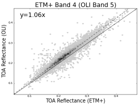
1. Introduction
The Landsat Thematic Mapper (TM) and Enhanced Thematic Mapper (ETM+) instruments, aboard the Landsat series of satellites, have been observing the land surface since the launch of Landsat-4 in 1982. Landsat-5 was launched in 1984, carrying an identical TM instrument, and Landsat-7 was launched in 1999, carrying the successor ETM+ instrument. These provide a broadly continuous record of satellite images of the land surface in six reflective wavelength bands, at a ground resolution of 30 m. The TM and ETM+ instruments sample the same regions of the spectrum, and while they have slightly different relative spectral response functions, they are often considered to be equivalent. Teillet et al. [1] provide a review of the continuity issues between these two instruments. More generally, Markham and Helder [2] provide a comprehensive review of efforts to create a radiometrically consistent calibration of all the Landsat instruments.
On 11 February 2013, the next in the Landsat series was launched. Initially known as the Landsat Data Continuity Mission (LDCM), it took the name Landsat-8 when handed over to the U.S. Geological Survey (USGS) for operational work on 30 May 2013. It was placed in its operational orbit on 12 April 2013, and all imagery collected from that date is considered operational, and made available as such by the USGS.
Landsat-8 carries a new instrument called the Operational Land Imager (OLI), which, while designed to be continuous with ETM+ and TM, also attempts to improve the instrument slightly [3]. In particular, the equivalent bands in the near infrared wavelengths have been narrowed significantly, to avoid some atmospheric attenuation features, which should provide for measurements which are much less affected by atmospheric variation, notably water vapour.
Due to the addition on the OLI instrument of an extra band at the blue end of the spectrum, the band numberings have changed between the instruments, and so care is taken in what follows to clearly distinguish band numbering. TM and ETM+ bands numbered 1, 2, 3, 4, 5, 7 are the reflective bands, and these correspond to OLI bands 2, 3, 4, 5, 6, 7 respectively.
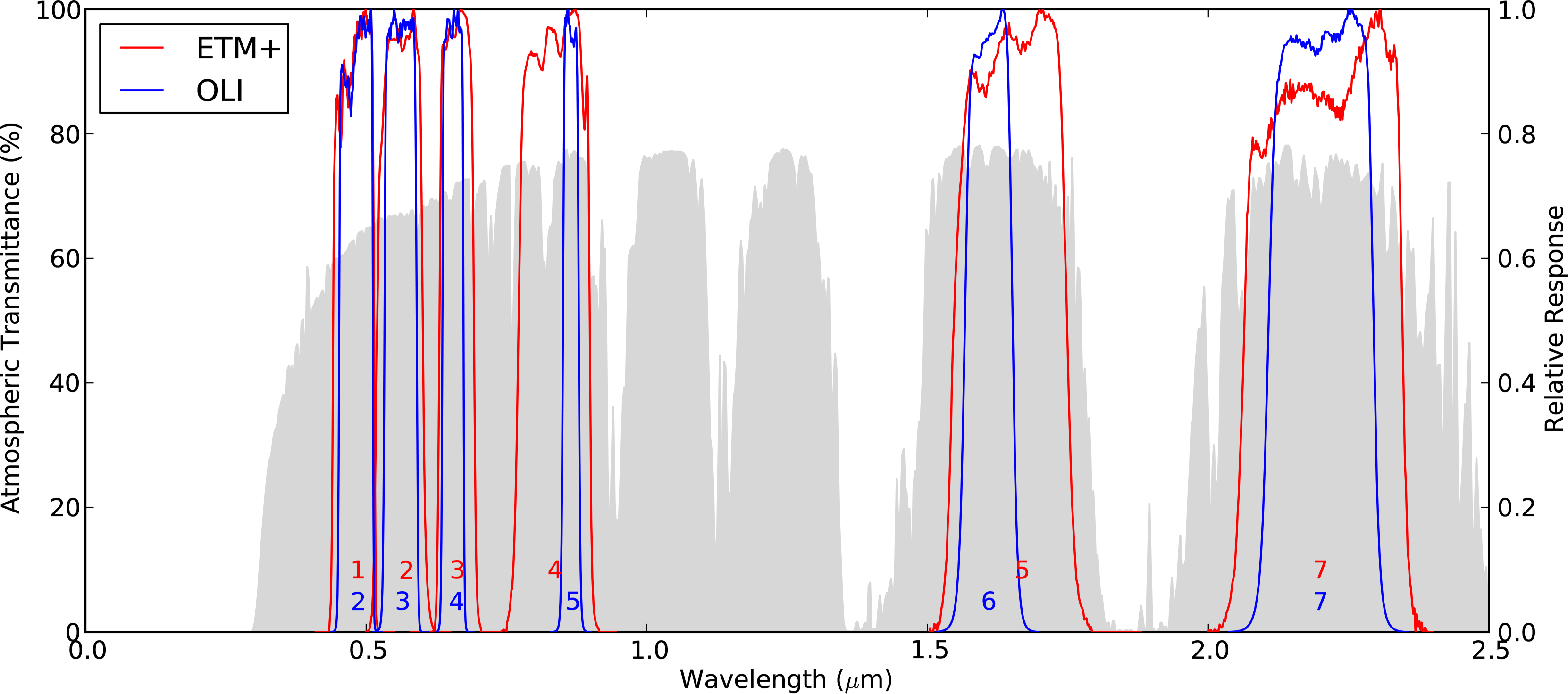
Figure 1 shows the relative spectral response functions for the equivalent reflective bands of the ETM+ and OLI instruments [4–6]. Also included is a generic representation of the atmospheric transmittance as a function of wavelength, modelled using the Second Simulation of the Satellite Signal in the Solar Spectrum (widely known as 6S) [7]. Atmospheric parameters were selected as fairly typical for Australian skies.
The spectral response of the OLI bands 5 and 6 is markedly narrower than for the corresponding ETM+ bands (4 and 5), and shows the avoidance of the atmospheric features within the ETM+ band windows.
The long timeseries of Landsat TM/ETM+ imagery has been of great use in monitoring the land surface [8–10]. Many workers have fitted models of biophysical parameters to the reflectance values, to transform reflectance into quantities of more physical significance. For example, Armston et al. [11]have fitted a model of overstorey foliage projective cover to top-of-atmosphere reflectance from Landsat-5 and Landsat-7. Scarth et al. [12] modelled fractional vegetation cover as a function of top-of-atmosphere reflectance from Landsat-5 and Landsat-7, and later re-fitted to surface reflectance (using the methods outlined by Guerschman et al. [13]). Other biophysical models based on reflectance data include the Tasselled Cap [14] and the forest disturbance index [15]. Other vegetation indices such as the Normalized Difference Vegetation Index (NDVI) are also used to model vegetation [16].
The changes in the spectral response in the OLI instrument could conceivably be sufficiently large to require that such models be re-fitted to the new imagery. Even for models not directly fitted to imagery, the change in sensor could cause a discontinuity in the time series which may be large enough to be a source of unwanted variability. For models which were fitted directly to image data, such re-fitting will require the collection of new field data, since any field data collected before the launch of Landsat-8 cannot be used directly for this purpose. Given the investment in existing models, it is worth assessing whether OLI reflectance data can be used as input to these models, and how important the differences may be.
The changes in reflectance values with the new instrument are not solely a function of the change in spectral response, because they also depend on the nature of the target. For example, a target which reflects only in the upper part of the ETM+ band 4 window, and not in the lower part, may be unaffected by the change to the OLI band 5, which does not sample that part of the spectrum at all. Naturally such a clear cut case will be unlikely, but more subtle cases may be quite common.
Li et al. [17] present a small study of several small plots in south-east Asia, comparing surface reflectance and a number of vegetation indices between the ETM+ and OLI sensors, and show that there are some subtle but notable differences in both reflectance and in vegetation indices, depending not only on the land type but also on the date pair on the same land type.
Thus, in order to test whether the changes are important, in terms of biophysical models, we must test on real imagery collected from the land surfaces of interest. The work which follows has focused on imagery for Australia, and tested two models of biophysical variables which are commonly used in the Australian context, one based on top-of-atmosphere reflectance and the other based on surface reflectance. These two cases show rather different characteristics in the differences between instruments.
2. Methods
2.1. A Comparison Dataset
The orbits of Landsat-7 and Landsat-8 are such that they alternately revisit each path 8 days apart. We make the assumption that 8 days is a sufficiently small interval that during this period only minor changes will occur on the ground, and they will not be consistently in one direction or the other. Pairs of dates were selected, per path/row, separated by 8 days, such that both images were cloud free. These pairs are thus assumed to be observations of the same target surface, one from Landsat-7 and one from Landsat-8, and so any differences between these two images are assumed to be due to the difference in sensor.
Two other possible schemes were considered. One was to use the data from the tandem overflight period, when Landsat-8 was flown in an orbit very close to that of Landsat-7 (29 and 30 March 2013), so that they viewed the same areas simultaneously, however the only data available in Australia from this period was severely cloud affected. The other possible scheme was to use the overlap area of two adjacent paths, which are flown on consecutive days. This would mean they were acquired much closer together in time, but they would be viewed under different angular conditions, and so may be subject to differences due to effects of the Bi-directional Reflectance Distribution Function (BRDF). While the imagery to be used has been corrected for BRDF effects, this correction was done using an average parameterization, constant over all pixels, and it was feared that the overlap areas could still be affected by per-pixel variation which may confound the analysis of sensor differences.
The cloud amount on each image was assessed using the Fmask algorithm of Zhu and Woodcock [18]. Complete absence of cloud was required, rather than just using the cloud mask to remove cloud affected pixels, in order to reduce the likelihood of contamination by undetected cloud or cloud shadow. Cloud edges can be difficult to detect precisely, and cloud shadow is more difficult to detect reliably, particular in the case of Landsat-7, with its gaps due to the failed scan-line corrector.
The radiometric processing methods used are exactly the same as were used historically to create the reflectance values which were originally used to fit the biophysical models which are included in the analysis. It is not known whether the biophysical models would be sensitive to a change in reflectance calculation, but this is not a factor in the current analysis. Most importantly, the same methods are used for both Landsat-7 and Landsat-8, so that the between-sensor differences being discussed here are not artifacts of different processing.
Two separate analyses were performed: one for top-of-atmosphere (TOA) reflectance (also known as at-sensor reflectance); and one for surface reflectance, after performing an atmospheric correction. For reasons which will become clear, these two cases have quite different characteristics.
Both Landsat-7 and Landsat-8 imagery are first converted to radiance values, using the coefficients supplied by the USGS (see Section 3 on data source). The radiance values are then converted to top-of-atmosphere or surface reflectance respectively (further details below). In all cases (Landsat-7/Landsat-8 and TOA reflectance/surface reflectance), the reference solar irradiance spectrum used is the Chance-Kurucz spectrum, as supplied with MODTRAN4 [19] (note that MODTRAN4 was not used for any other purpose in the current study). This spectrum was originally chosen because it had been used by the Landsat Science Team for testing of ETM+ [20]. For the current study, it is important that a consistent solar spectrum be used, as a change in reference solar irradiance spectrum can be responsible for substantial differences in reflectance values, depending on the band in question [20,21].
In both cases the imagery was corrected (by different methods) for the effects of the angular configuration of sun, surface and satellite, however, because each pair was acquired under roughly the same angular configuration, it is believed that this is of minimal importance in the current study, as each image of the pair would be subject to the same angle correction factor.
In the case of the TOA reflectance, the correction used the methods described by Danaher et al. [22]. This approach uses a single model of the variation of TOA reflectance with sun and satellite position to adjust to a standard angular configuration. This model implicitly assumes a constant atmosphere, and rolls the correction of atmospheric effects and BRDF effects into a single function of angular configuration. A simple topographic correction is also applied to the resulting standardised TOA reflectance, using the methods of Dymond and Shepherd [23].
The surface reflectance imagery was corrected for atmospheric effects and angular configuration using the methods of Flood et al. [24]. Briefly, this method uses 6S [7] to correct for atmospheric effects, and a BRDF model (with constant parameters) to adjust surface reflectance to a standard angular configuration. The spectral response functions shown in Figure 1 were added to the 6S sensor library for the conversion to surface reflectance. The atmospheric parameterization includes estimates of ozone from seasonal climatology, estimates of total column water vapour from daily ground humidity measurements, and a small, fixed value for aerosol optical depth. The latter is believed to be sufficient under Australian skies due to their commonly low aerosol loading, as analysed in detail by Gillingham et al. [25]. Other aerosol estimation methods have been found to be less accurate in Australia, due to the relative brightness of the vegetation [26]. The BRDF model is applied using angles calculated from the local topography of each pixel, and thus also provides a correction for topographic illumination effects as well as sun and sensor position.
Pairs of dates were selected for a total of 123 distinct path/rows, and a subset of 12 of these path/rows (chosen randomly from the whole set) was set aside as validation areas. No pixels from these areas were used in model fitting, and all comparisons were performed using only pixels from these validation areas. Further detail on the data selection is given in Section 3.
A subset of pixels was selected in a regular grid across these scenes, and the reflectance values extracted, for all reflective bands.
In comparing the agreement of the two sensors, several methods were used. Scatter plots of reflectance from the corresponding bands of the two sensors were made, showing graphically the agreement between the two. Two measures of agreement were calculated. Firstly, the mean absolute difference (MAD) was used to quantify the absolute amount of difference between the reflectance values. Secondly, the systematic bias between the two was characterised using the slope of a regression line forced through the origin. The regression was calculated using orthogonal distance regression (ODR), which does not favour one variable over the other. This slope value gives a measure of the average proportional change between the two sensors. A perfect agreement between the sensors would have a mean absolute difference of zero, and a regression slope of 1.
It should be noted at this point that the use of ODR regression in this contexts is purely as a simple measure of the average relative change between the two sensors. This is quite distinct from using a regression model to estimate one sensor from a measurement of the other, which is done using ordinary least squares regression (OLS), as described in Section 2.3. ODR assumes that there is noise in either variable, and so does not bias towards one or the other, which is appropriate when simply looking at the relative difference between the two. OLS regression assumes that all unmodelled variation is in the dependant variable, while the independant variable is an exact measurement. This is appropriate when using measurements from one sensor to estimate measurements from the other.
2.2. Biophysical Models
In order to assess the impact of the difference in reflectance, two models of biophysical quantities were used, to understand how a small difference in reflectance translates to a difference in the biophysical quantity. In the case of TOA reflectance, an existing multiple linear regression model of overstorey foliage projective cover (FPC) was used. This model had been fitted on Landsat-7 ETM+ TOA reflectance imagery, to predict overstorey foliage projective cover in the Australian landscape [11], and is used in a number of vegetation management applications in Australia [27]. Overstorey foliage projective cover is defined as “the vertically projected percentage cover of the photosynthetic foliage from tree and shrub life forms greater than 2 m height” [11], and is a measure of the tree cover at a particular location. Armston et al. [11] discuss the relationship between FPC and other measures such as leaf area index or crown cover, and why FPC is an appropriate measure of Australian vegetation. This model makes use of all the ETM+ reflective bands except band 1, which is omitted due to its greater sensitivity to aerosol contamination.
For the surface reflectance, we used a model of fractional vegetation cover, originally fitted to historic Landsat-5 TM and Landsat-7 ETM+ top-of-atmosphere reflectance imagery and field-surveyed cover data by Scarth et al. [12], and more recently re-fitted to surface reflectance imagery [13]. This uses a spectral unmixing approach to calculate three vegetation cover fractions, for the fraction of land surface covered by bare soil, green (i.e., photosynthesizing) vegetation, and non-photosynthesizing vegetation. This model also makes use of all the ETM+ reflective bands except band 1. As for the FPC model, band 1 is omitted due to its greater sensitivity to aerosol contamination.
Since the NDVI is also widely used for monitoring vegetation density, this is also compared, between the two sensors, using the surface reflectance imagery. NDVI is a ratio of the red and near-infrared reflectances, discussed in a review by Bannari et al. [16]. In terms of ETM+ bands, it is generally calculated as
In each case, the model in question was applied to the Landsat-7 and Landsat-8 reflectance values, and the resulting values compared in the same way as for reflectance, using scatter plots, MAD and ODR regression slope.
2.3. Predicting ETM+ from OLI
The reflectance data from the training scenes was used to fit an ordinary least-squares linear regression relationship to predict Landsat-7 ETM+ reflectance from the reflectance in the equivalent band of Landsat-8 OLI. As discussed in Section 2.1, this is quite distinct from the ODR slopes used as a simple measure of average relative difference between sensors. In Equation (2), the reflectances are given as ρETM+ and ρOLI, with the regression coefficients c0 and c1. This relationship allows us to take reflectance values from OLI, adjust them to be more like ETM+ reflectances, and then use those in models which were originally fitted to ETM+ data. The chosen regression was univariate for each band. A multivariate case was also tested, in which each band of ETM+ was predicted from all bands of OLI, but this did not result in a useful improvement in the prediction, and is not included here.
The resulting adjusted reflectances were used in each of the biophysical models discussed above, and the resulting adjusted biophysical parameters compared between the two sensors, as before, to assess the value of the adjustment.
2.4. Regional Variability of the Difference
A separate sub-analysis was performed, in order to investigate the extent to which results are consistent across regions. Since, as noted above, the effects depend on the nature of the target, it is likely that results will vary from one region to another. In order to ascertain the extent of this variability, the same comparison between ETM+ and OLI was performed on subsets of the data, grouped by their WRS-2 path. The path was chosen simply as a convenient means of grouping imagery on a regional basis, rather than for any special significance. The resulting comparisons each give a regression slope (ODR regression) as a measure of the average bias between the two sensors, for each band.
3. Data
All imagery used in this work was downloaded from the US Geological Survey website [28]. The Landsat-8 OLI imagery included the calibration changes made by the Landsat Science Team on 3 February 2014. The data covers the range of dates from the start of operational scanning by Landsat-8 up to the latest date available at the time of the analysis (cloud free dates were found in the range from 11 April 2013 to 12 January 2014). This covers nearly a full year, and hence a range of seasonal variation.
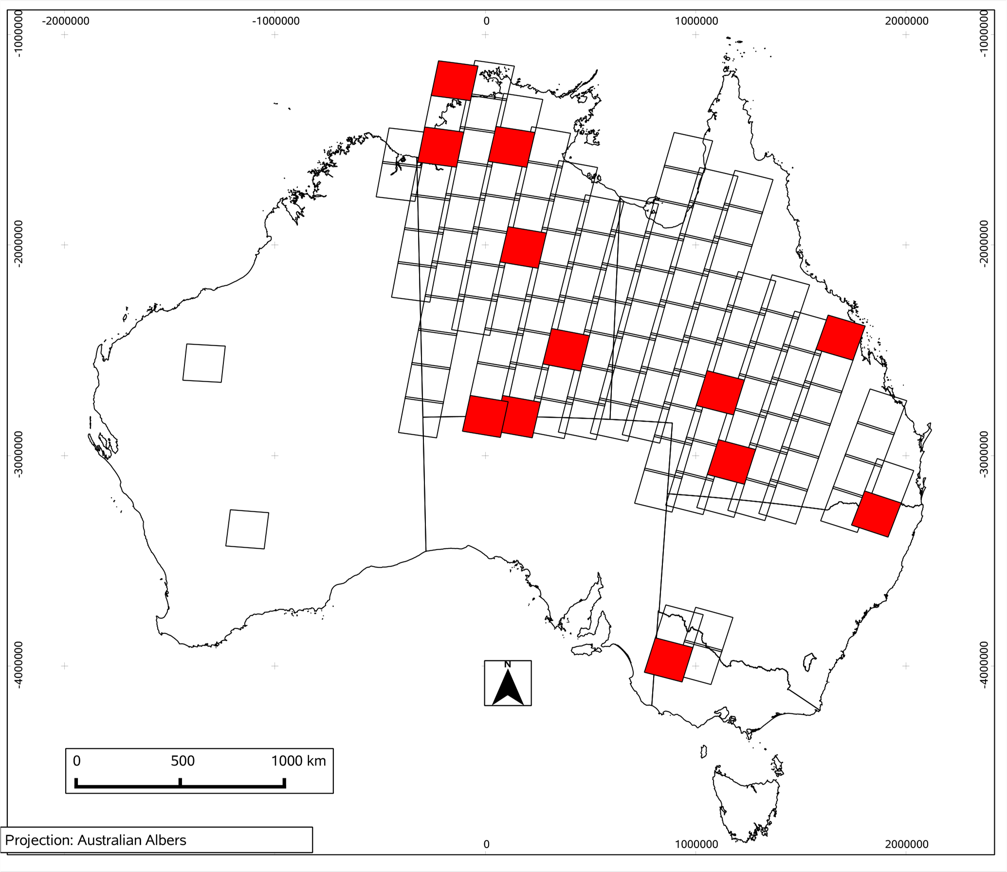
Data available in the Queensland Remote Sensing Centre archive covered the Australian states of Queensland, Northern Territory and Victoria, with a small number of scenes also available in Western Australia and New South Wales. There were 123 scenes, with 793 distinct pairs of dates. Of these, 12 scenes (10% of scenes) were randomly selected to use for validation only, and the remaining 111 scenes were used for fitting ETM+ prediction models. The scenes are shown in Figure 2, with the red scenes being those used for validation. The locations cover a wide range of the land types present in Australia, including sub-tropical rainforest, open savannah, and desert.
Pixels were selected on a regular grid across each scene (excluding water bodies) with approximately 400 points per scene, over all dates, resulting in a total of 347,562 pairs for training and 26,230 pairs for validation.
All analyses shown below include only points from the validation scenes.
4. Results
All scatter plots shown in this section are density plots, so that the darker areas of the graph show more points in that region. Light grey areas show relatively few points (as few as one), while black areas indicate that many more points are present in that region of the graph.
4.1. Top-of-Atmosphere (TOA) Reflectance and Foliage Projective Cover (FPC)
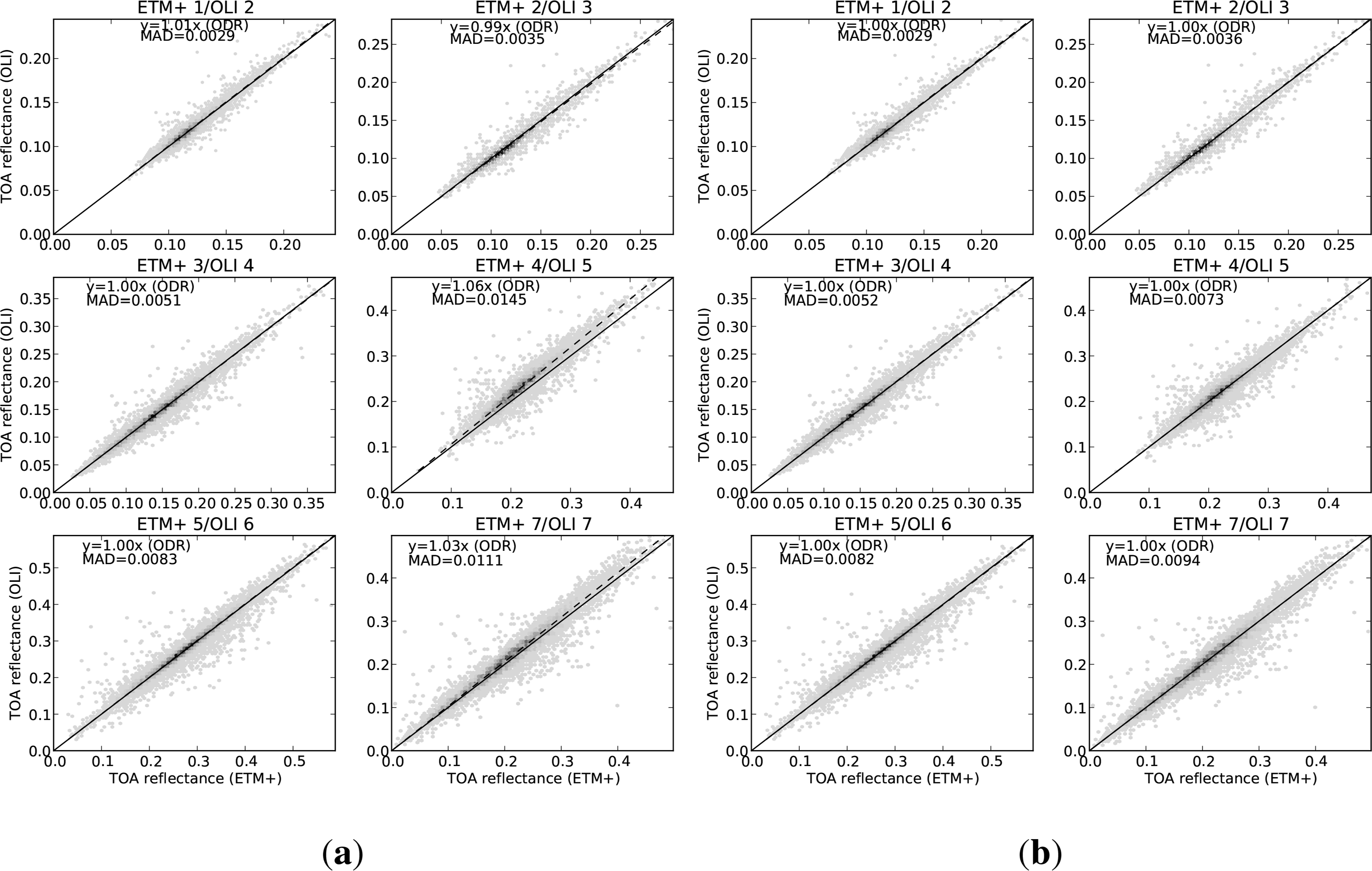
Figure 3a shows the TOA reflectance for corresponding bands of Landsat-8 OLI and Landsat-7 ETM+. They show some scatter on the plots, and the ODR slope values show that there is also a systematic overall difference between the two instruments, although this is much stronger in some bands than others. The scatter would mainly arise from two sources. Firstly, there would be the between-sensor differences which vary depending on the nature of the target, and can be assumed to be different for each pixel. Secondly, there would be those pixels which have changed between the two observations, violating the assumption of no change, discussed in Section 2.1. It is assumed that this is a minor component of the scatter.
The largest systematic change (around 6%) is in ETM+ 4 (OLI 5), which has a much narrower window in OLI than in ETM+. It should be noted that this band is in the part of the spectrum which is fairly strongly affected by atmospheric attenuation (as shown in Figure 1), and the dependence of the atmospheric effects on wavelength is stronger in the part of the window which has been removed, especially with the avoidance of the water vapour absorption feature at 0.825 μm. This means that the strong effect here includes the interaction between the change in window and the atmospheric attenuation. As will be seen in Section 4.2, this strong change in this band is not apparent in the surface reflectance case.
Band ETM+ 5 (OLI 6) also has a markedly narrower window, but shows surprisingly little change in reflectance. On the other hand, ETM+ 7 (OLI 7), in which the strongest response in the ETM+ window (wavelength >2.3 μm) has been almost entirely excluded from the OLI window, also shows a larger change, of around 3%.
Figure 3b shows the same data, after applying the regression (Table 1) to predict ETM+ reflectance from the OLI values. The regression coefficients were created using only points from the training dataset, and none from this validation dataset. In the two bands with the greatest change (ETM+ 4 and 7), the OLI slope values are now equal to 1.00, and the MAD values have been reduced. In all the other bands, which showed very little between-sensor difference, the reflectance values are only marginally changed.
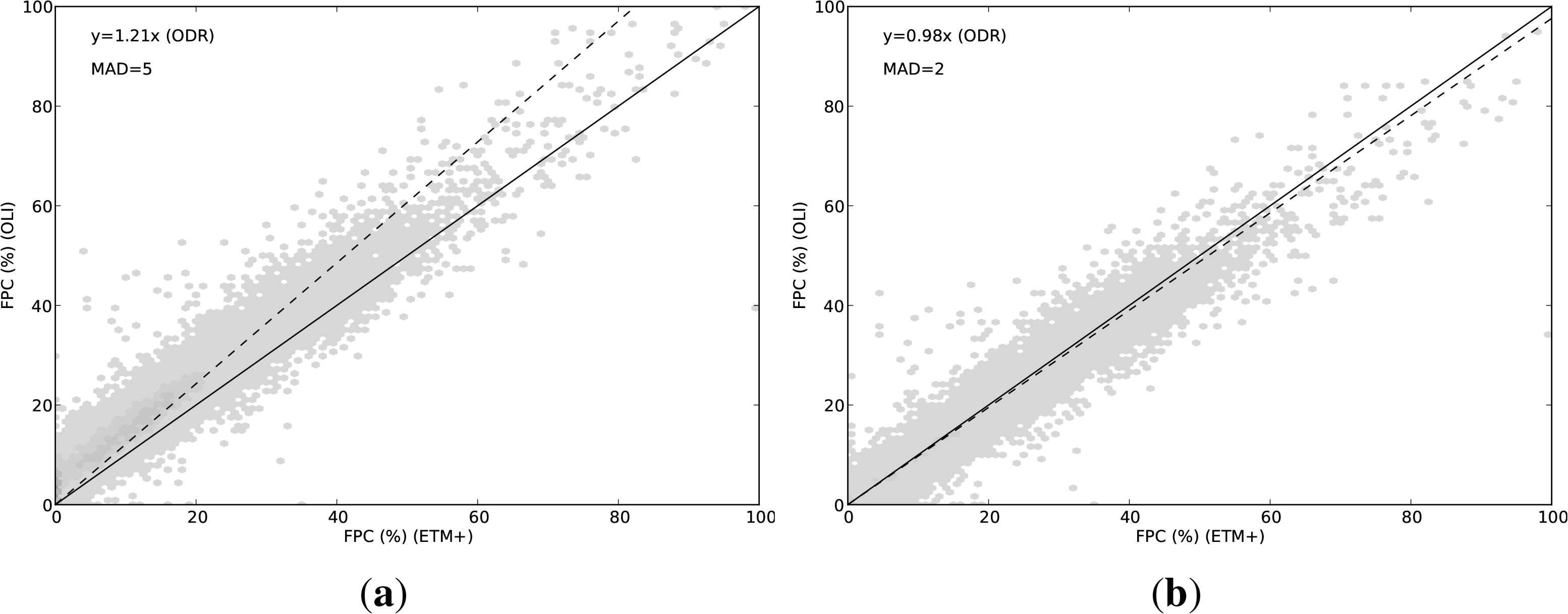
Figure 4a shows the effect of the between-sensor difference on FPC, and Figure 4b shows the effect of adjusting the OLI reflectance values to match ETM+. Without adjusting the OLI reflectances, there is a clear between-sensor difference in the modelled FPC, amounting to an increase of several percentage points. Using the adjusted OLI reflectance values, the FPC values match much more closely, with the ODR slope being very much closer to 1. It should be emphasized that the adjustment is performed on the reflectance values, without regard to the FPC model.
4.2. Surface Reflectance and Fractional Cover and NDVI
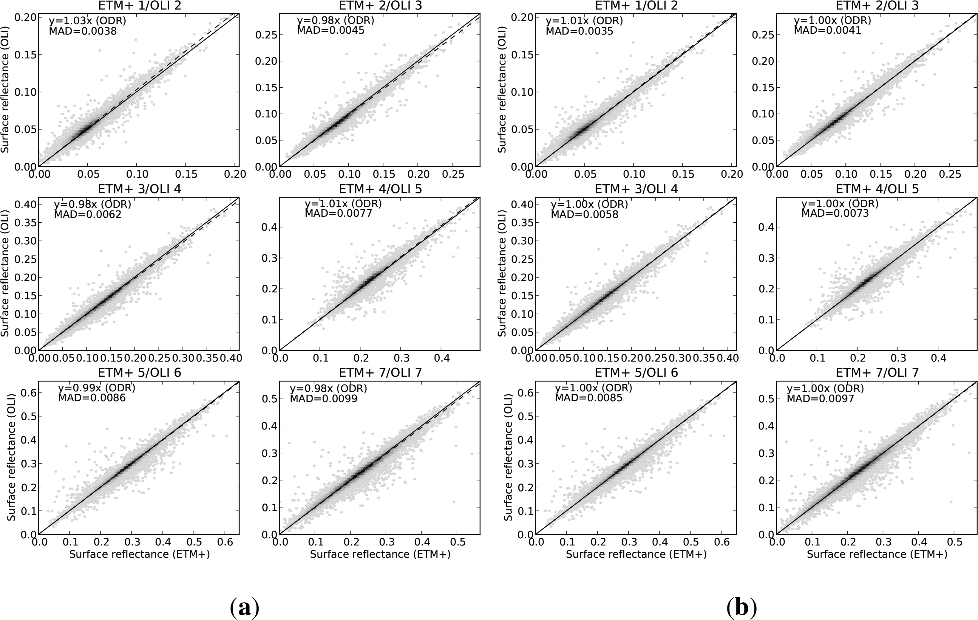
Figure 5a shows the surface reflectance for corresponding bands of Landsat-8 OLI and Landsat-7 ETM+. The amount of scatter is similar to the TOA case, but the systematic bias indicated by the ODR slope shows that in the surface reflectance case, all bands are affected by some between-sensor difference, with all ODR slope values being either greater or less than 1. As discussed in Section 4.1, the larger between-sensor difference in band ETM 4 (OLI 5) is not evident in the surface reflectance, due to the removal (by atmospheric correction) of the stronger wavelength dependent atmospheric attenuation across the spectral window, including the water vapour absorption feature. The largest change, in ETM+ band 1 (OLI 2), is around 3%, and the other bands are all either 1 or 2%.
Figure 5b shows the same reflectance data, after applying the regression (Table 2) to predict ETM+ surface reflectance from the OLI values. As discussed earlier, these points were not used in fitting the regression. The ODR slope for ETM+ band 1 (OLI 2) is now 1.01, and in all other bands it is 1.00, showing much better agreement between sensors.
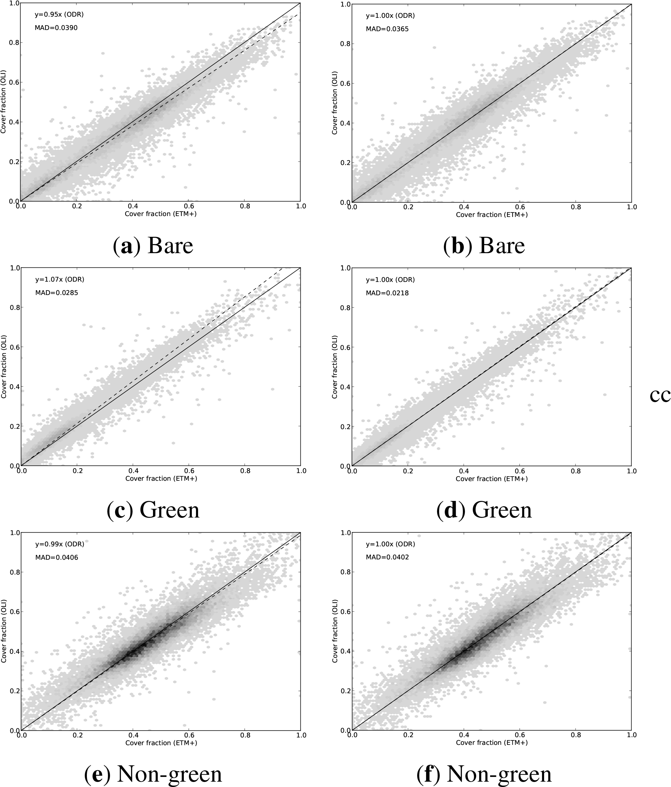
Figure 6a shows the effect of between-sensor difference on the fractional cover model. With no adjustment, there is a systematic difference in the bare fraction and the green fraction, while the non-green fraction agrees much more closely. The bare fraction calculated from the OLI underestimates that calculated from ETM+ by about 5%, while the green fraction is overestimated by 7%. If the adjusted OLI reflectances are used instead, as shown in Figure 6b, the resulting systematic error is reduced, with all the ODR regression slopes being equal to 1.00. Again, it should be emphasized that the empirical adjustment being made to the OLI values is made solely in terms of reflectance, without regard to the fractional cover model.
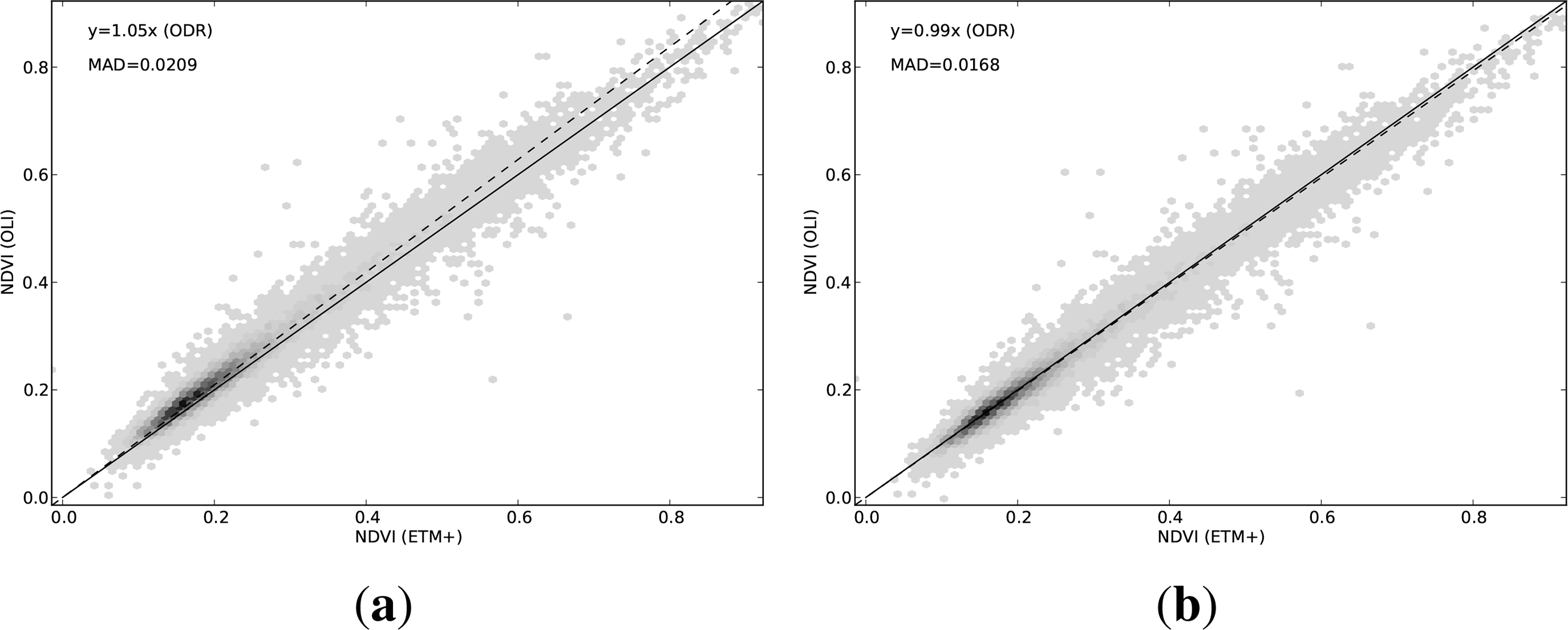
Figure 7a shows the between-sensor difference in NDVI. Without any adjustment of the reflectance values, the OLI appears to systematically overestimate NDVI by about 5%, relative to ETM+. Using the adjusted reflectances, Figure 7b, the NDVI values agree within 1%, on average, with the ODR regression slope equal to 0.99.
4.3. Consistency of the Between-Sensor Change
As described in Section 2.4, comparisons were also performed for subsets of the full dataset, grouped by the WRS-2 path of the images. For each path, for each band, the ODR regression slope relating ETM+ and OLI was computed, to see how variable this is between regions. These results are summarised in Tables 3 and 4. Note that these use all of the extracted points for that path, and are not the same subsets as either the training or validation datasets discussed above, hence the values are not expected to be identical to those shown in the reflectance scatter plots.
For each path, the ODR regression slope between OLI and ETM+ is given for each band. The number of extracted points is also given. Also included in these tables is the ODR regression slopes when all datapoints from all paths are pooled together (path given as “all”).
These tables show that there is some variation between paths, which supports the suggestion made in the introduction that the relationship between sensors depends on the target. However, there is a degree of consistency. When the slopes for all paths together are a little greater than 1, the slopes for the individual paths are also generally a little greater than 1, rather than being sometimes greater and sometimes less. The exceptions to this are for paths where the number of data points available is considerably smaller, such as path 090 (only two rows included). This suggests that when attempting to quantify an average adjustment in this manner, it is important to use more than just a few scenes, otherwise the effect will be dominated by more local effects, which would not then apply outside that region.
5. Discussion
The reflectance adjustments demonstrated in Figures 3 and 5 show that there is a systematic difference between the two sensors, which can reliably be removed over large areas. The scatter plots also show that there is a remaining component, sometimes larger than the systematic difference, which varies per pixel, which cannot be removed by the methods discussed here. This remaining difference is quantified in the values of MAD for the adjusted OLI reflectance plots.
The systematic component of the between-sensor difference is much smaller in the surface reflectance than in top-of-atmosphere reflectance. This is because some of the difference is due to atmospheric effects interacting with the change in spectral response of the instrument, and the atmospheric correction is able to account for these differences directly, by proper modelling of the radiative transfer through the atmosphere. This means that the continuity between ETM+ and OLI is much better when dealing with surface reflectance.
The models of biophysical variables used here are both strongly non-linear functions of reflectance, and the impact of a small change in reflectance is not easily predictable. The tests shown in Figures 4 and 6 demonstrate that the between-sensor difference in reflectance can indeed translate through to a difference in the biophysical variable being modelled, but also that a systematic adjustment of the reflectance will also result in an improvement in the continuity of the modelled variable. However, this is only true on average, over all pixels, and as with reflectance, there remains a component of between-sensor difference which is not adjusted for by this sort of procedure.
It should be emphasised that there are other possible sources of variation between the image pairs used here. These include: mis-registration between images; variations in atmospheric conditions not accounted for by the atmospheric parameterisation; change in the land surface between the dates of the pair; BRDF effects not accounted for by the constant parameterisation of the BRDF model. Of these, some are more important than others. The registration methods used by the USGS in their processing are very good, and the image-to-image registration error is very much less than one pixel. The Landsat-7 Image Assessment System [29] estimates the image-to-image registration error to be on the order of 3.5 m, and that for Landsat-8 should be less, given the improved techniques used. The most troublesome atmospheric parameter is likely to be aerosol optical depth, used in the atmospheric correction to surface reflectance, and as discussed in Section 2.1, Gillingham et al. [26] have analysed this under Australian conditions and concluded that this should mostly be a small problem, due to Australia’s relatively clear skies. Changes in the land surface between dates are assumed to be negligible, due to the short time period between images (8 days), but there is no way to assess this rigorously. Differences in BRDF between images are assumed to be negligible, because in 8 days, the angular configuration of sun and satellite is very nearly unchanged. Most importantly, all of these possible sources of variation seem unlikely to act systematically in one direction or another, and can therefore be assumed to contribute only to the scatter, and not to the systematic bias.
The between-path variability of the between-sensor difference, as highlighted in Section 4.3, suggests that regional differences in even the systematic component may be important. Certainly, it strongly suggests that an adjustment based on a small number of scenes should not be presumed to apply outside that area. On the other hand, it does raise the possibility of whether a per-scene adjustment may be more appropriate. In order to test this, it would be valuable to have a much longer record of coincident ETM+ and OLI data, in order to sample a wider range of variation. This could be used to test whether a local adjustment for that region was consistent over time. In the extreme, one might consider a very long series of data to allow a per-pixel fitting of the adjustment, but this would probably be counter-productive. If the characteristics to be corrected are so detailed as to require per-pixel parameterization, they would also be such as to change when the pixel characteristics changed, and so would require re-fitting on a regular basis. This is difficult to do with the 16 day revisit cycle of Landsat, and would work against the whole point of using Landsat to monitor change. Similarly, a characterization of the relationship stratified by land type requires prior land type classification, and would seem open to being confounded by a change in the land surface (e.g., clearing some forest cover) as one would apply the wrong correction for that class. To investigate what sort of stratification (if any) might be ultimately beneficial in reducing the between-sensor variation, and whether the classes could be determined directly from each image prior to adjustment, seems likely to be a substantial piece of research work for the future, and may need to be undertaken specifically for the area of interest.
Section 4.3 also raises questions as to how applicable the current adjustment coefficients would be to other parts of the world. Whilst the degree of consistency suggests that it should be reasonable to apply them to other paths within Australia, this may not be true with regard to applying them to other continents. In particular, areas with vegetation communities or soil types radically different to those represented here may present significantly different spectral response, and thus require significantly different adjustment of OLI to maintain continuity with ETM+. Hence, a similar procedure should be considered using imagery from the area of interest.
It seems likely that the fine detail of the radiometric processing used here is not a critical factor in the adjustment coefficients calculated. The major between-sensor effects are from relatively gross changes in the spectral windows, and so, for example, it seems likely that the same effects would appear if a different reference irradiance spectrum were used, so long as it had been used consistently, and that the per-pixel and per-region differences discussed above would be much larger sources of variation. However, it should be noted that the current work has not rigorously tested this.
All of the analysis performed here was carried out on land pixels, and does not include any pixels with open water, such as ocean, lakes or rivers. It seems likely that the behaviour of reflectance would be quite different, but this is not addressed in the current work.
6. Conclusions
This study of ETM+ and OLI reflectance in the Australian landscape suggests that the differences between the two sensors may be large enough to warrant action, in some contexts, particularly when using biophysical models which have already been fitted to existing field data and coincident ETM+ imagery. It is shown that this difference is more pronounced when using top-of-atmosphere reflectance than atmospherically corrected reflectance. While the difference is highly variable between bands, in the case of top-of-atmosphere reflectance, the average difference can be as much as 6% of the reflectance, and the surface reflectance can be affected by up to 2%. A simple empirical procedure is developed which estimates ETM+ reflectance from OLI reflectance, for both top-of-atmosphere and surface reflectance cases. This procedure only removes that part of the between-sensor difference which is systematic across the landscape, and there remains a notable difference which is much more localized (probably per-pixel), and it is not clear from the current work how this remaining component might be addressed. However, the removal of the systematic component of the between-sensor difference does markedly improve the continuity of existing models of biophysical parameters when applied to the new OLI reflectance data. The impact on biophysical models depends on the sensitivity of the particular model in question. In the models discussed here, the Foliage Projective Cover model, using top-of-atmosphere reflectance, shows a between-sensor difference of at least 10%, which is reduced to less than 2% by adjusting the OLI reflectances. The fractional cover model, using surface reflectance, shows differences of up to 7%, which is reduced to less than 1% by adjusting the reflectances. The value of NDVI is affected by around 5% on average, and adjusting the OLI surface reflectances reduces this systematic between-sensor difference to around 1%. In view of the dependence of such models on the sensor, it is recommended that, as more OLI imagery becomes available, and more field data is collected to coincide with it, it would be preferable to re-fit such models directly to OLI reflectance data, which may remove more of the between-sensor differences.
Acknowledgments
The author would like to thank Robert Denham, Peter Scarth, Tim Danaher, John Armston and Tony Gill from the Joint Remote Sensing Research Program for discussions on the methodology. The Joint Remote Sensing Research Program is supported financially by the governments of the Australian states of Queensland, New South Wales and Victoria.
Conflicts of Interest
The author declares no conflict of interest.
References
- Teillet, P.; Barker, J.; Markham, B.; Irish, R.; Fedosejevs, G.; Storey, J. Radiometric cross-calibration of the Landsat-7 ETM+ and Landsat-5 TM sensors based on tandem data sets. Remote Sens. Environ 2001, 78, 39–54. [Google Scholar]
- Markham, B.L.; Helder, D.L. Forty-year calibrated record of earth-reflected radiance from Landsat: A review. Remote Sens. Environ 2012, 122, 30–40. [Google Scholar]
- Irons, J.R.; Dwyer, J.L.; Barsi, J.A. The next Landsat satellite: The Landsat data continuity mission. Remote Sens. Environ 2012, 122, 11–21. [Google Scholar]
- Barsi, J.A.; Markham, B.L.; Pedelty, J.A. The operational land imager: Spectral response and spectral uniformity. Proc. SPIE 2011, 8153, 81530G-81530G–11. [Google Scholar]
- Landsat-8 Relative Spectral Reponse. Available online: http://ldcm.nasa.gov/docs/Ball_BA_RSR.v1.1.xlsx (accessed on 8 June 2012).
- Landsat-7 Relative Spectral Response. Available online: https://landsat.usgs.gov/documents/L7_RSR.xlsx (accessed on 18 March 2014).
- Vermote, E.; Tanre, D.; Deuze, J.; Herman, M.; Morcette, J.J. Second simulation of the satellite signal in the solar spectrum, 6S: An overview. IEEE Trans. Geosci. Remote Sens 1997, 35, 675–686. [Google Scholar]
- Hansen, M.C.; Loveland, T.R. A review of large area monitoring of land cover change using Landsat data. Remote Sens. Environ 2012, 122, 66–74. [Google Scholar]
- Cohen, W.B.; Goward, S.N. Landsat’s role in ecological applications of remote sensing. BioScience 2004, 54, 535–545. [Google Scholar]
- Kennedy, R.E.; Andréfouët, S.; Cohen, W.B.; Gómez, C.; Griffiths, P.; Hais, M.; Healey, S.P.; Helmer, E.H.; Hostert, P.; Lyons, M.B.; et al. Bringing an ecological view of change to Landsat-based remote sensing. Front. Ecol. Environ 2014, 12, 339–346. [Google Scholar]
- Armston, J.D.; Denham, R.J.; Danaher, T.J.; Scarth, P.F.; Moffiet, T.N. Prediction and validation of foliage projective cover from Landsat-5 TM and Landsat-7 ETM+ imagery. J. Appl. Remote Sens 2009, 3, 033540–033567. [Google Scholar]
- Scarth, P.; Röder, A.; Schmidt, M. Tracking grazing pressure and climate interaction—The role of Landsat fractional cover in time series analysis. In Proceedings of the 15th Australasian Remote Sensing and Photogrammetry Conference, Alice Springs, Australia, 13–17 September 2010; pp. 936–948.
- Guerschman, J.P.; Scarth, P.; McVicar, T.R.; Malthus, T.J.; Stewart, J.B.; Rickards, J.E.; Trevithick, R.; Renzullo, L.J. Assessing the effects of site heterogeneity and soil properties when unmixing photosynthetic vegetation, non-photosynthetic vegetation and bare soil fractions from Landsat and MODIS data. Remote Sens. Environ 2014. in press.. [Google Scholar]
- Crist, E.P. A TM tasseled cap equivalent transformation for reflectance factor data. Remote Sens. Environ 1985, 17, 301–306. [Google Scholar]
- Healey, S.P.; Cohen, W.B.; Yang, Z.; Krankina, O.N. Comparison of tasseled cap-based Landsat data structures for use in forest disturbance detection. Remote Sens. Environ 2005, 97, 301–310. [Google Scholar]
- Bannari, A.; Morin, D.; Bonn, F.; Huete, A.R. A review of vegetation indices. Remote Sens. Rev 1995, 13, 95–120. [Google Scholar]
- Li, P.; Jiang, L.; Feng, Z. Cross-Comparison of vegetation indices derived from Landsat-7 enhanced thematic mapper plus (ETM+) and Landsat-8 operational land imager (OLI) sensors. Remote Sens 2014, 6, 310–329. [Google Scholar]
- Zhu, Z.; Woodcock, C.E. Object-based cloud and cloud shadow detection in Landsat imagery. Remote Sens. Environ 2012, 118, 83–94. [Google Scholar]
- Berk, A.; Anderson, G.P.; Acharya, P.K.; Chetwynd, J.H.; Bernstein, L.S.; Shettle, E.P.; Matthew, M.W.; Adler-Golden, S.M. MODTRAN4 User’s Manual; Technical Report; Air Force Research Laboratory, Air Force Materiel Command: Hanscom Air Force Base, MA, USA, 2000. [Google Scholar]
- Landsat-7 Science Data Users Handbook. Available online: http://landsathandbook.gsfc.nasa.gov/data_prod/prog_sect11_3.html (accessed on 16 July 2014).
- Thome, K.; Biggar, S.; Slater, P. Effects of assumed solar spectral irradiance on intercomparisons of earth-observing sensors. Proc. SPIE 2001, 4540. [Google Scholar] [CrossRef]
- Danaher, T.; Wu, X.; Campbell, N. Bi-Directional reflectance distribution function approaches to radiometric calibration of Landsat ETM+ imagery. In Proceedings of the IEEE International Geoscience and Remote Sensing Symposium 2001 (IGARSS ’01), Sydney, Australia, 9–13 July 2001; 6, pp. 2654–2657.
- Dymond, J.; Shepherd, J. Correction of the topographic effect in remote sensing. IEEE Trans. Geosci. Remote Sens 1999, 37, 2618–2619. [Google Scholar]
- Flood, N.; Danaher, T.; Gill, T.; Gillingham, S. An operational scheme for deriving standardised surface reflectance from Landsat TM/ETM+ and SPOT HRG imagery for Eastern Australia. Remote Sens 2013, 5, 83–109. [Google Scholar]
- Gillingham, S.; Flood, N.; Gill, T. On determining appropriate aerosol optical depth values for atmospheric correction of satellite imagery for biophysical parameter retrieval: Requirements and limitations under Australian conditions. Int. J. Remote Sens 2013, 34, 2089–2100. [Google Scholar]
- Gillingham, S.; Flood, N.; Gill, T.; Mitchell, R. Limitations of the dense dark vegetation method for aerosol retrieval under Australian conditions. Remote Sens. Lett 2012, 3, 67–76. [Google Scholar]
- Danaher, T.; Scarth, P.; Armston, J.; Collett, L.; Kitchen, J.; Gillingham, S. Remote sensing of tree-grass systems: The Eastern Australian woodlands. In Ecosystem Function in Savannas: Measurement and Modelling at Landscape to Global Scales; Hill, M.J., Hanan, N.P., Eds.; CRC Press: Boca Raton, FL, USA, 2011; pp. 175–193. [Google Scholar]
- USGS Earth Explorer. Available online: http://earthexplorer.usgs.gov (accessed on 12 February 2014).
- Landsat-7 Image Assessment System, Geometric Algorithm Theoretical Basis Document. Available online: http://landsat.usgs.gov/documents/LS-IAS-01_Geometric_ATBD.pdf (accessed on 16 July 2014).


| Band | c0 | c1 |
|---|---|---|
| ETM 1 (OLI 2) | 0.00501 | 0.95852 |
| ETM 2 (OLI 3) | 0.00307 | 0.98911 |
| ETM 3 (OLI 4) | 0.00198 | 0.99291 |
| ETM 4 (OLI 5) | 0.00087 | 0.93819 |
| ETM 5 (OLI 6) | 0.00141 | 0.98824 |
| ETM 7 (OLI 7) | −0.00147 | 0.97591 |
| Band | c0 | c1 |
|---|---|---|
| ETM 1 (OLI 2) | 0.00041 | 0.97470 |
| ETM 2 (OLI 3) | 0.00289 | 0.99779 |
| ETM 3 (OLI 4) | 0.00274 | 1.00446 |
| ETM 4 (OLI 5) | 0.00004 | 0.98906 |
| ETM 5 (OLI 6) | 0.00256 | 0.99467 |
| ETM 7 (OLI 7) | −0.00327 | 1.02551 |
| ODR Regression Slope | |||||||
|---|---|---|---|---|---|---|---|
| WRS-2 Path | Num Pts | TM 1 | TM 2 | TM 3 | TM 4 | TM 5 | TM 7 |
| 090 | 1447 | 1.05 | 1.05 | 1.05 | 1.08 | 1.01 | 1.04 |
| 091 | 8704 | 1.01 | 1.01 | 1.02 | 1.10 | 1.01 | 1.06 |
| 093 | 10440 | 1.01 | 1.01 | 1.03 | 1.09 | 1.02 | 1.05 |
| 094 | 15403 | 1.00 | 0.98 | 0.99 | 1.07 | 1.00 | 1.04 |
| 095 | 18710 | 1.00 | 0.99 | 0.99 | 1.06 | 1.00 | 1.02 |
| 096 | 26419 | 1.01 | 0.99 | 0.99 | 1.06 | 1.00 | 1.01 |
| 097 | 38178 | 1.00 | 0.99 | 1.00 | 1.06 | 1.01 | 1.04 |
| 098 | 45880 | 1.00 | 0.99 | 1.00 | 1.06 | 1.01 | 1.02 |
| 099 | 34016 | 1.00 | 0.98 | 0.99 | 1.05 | 1.00 | 1.02 |
| 100 | 21467 | 1.00 | 0.98 | 0.99 | 1.05 | 1.01 | 1.02 |
| 101 | 24302 | 1.00 | 0.98 | 0.99 | 1.06 | 1.01 | 1.05 |
| 102 | 21200 | 1.00 | 0.98 | 0.99 | 1.05 | 0.99 | 1.00 |
| 103 | 23216 | 1.00 | 0.99 | 1.00 | 1.07 | 1.01 | 1.04 |
| 104 | 22993 | 1.00 | 0.98 | 0.99 | 1.06 | 1.01 | 1.04 |
| 105 | 33444 | 1.00 | 0.99 | 1.00 | 1.07 | 1.01 | 1.04 |
| 106 | 21471 | 1.00 | 0.99 | 1.00 | 1.06 | 1.01 | 1.04 |
| 107 | 1781 | 1.00 | 1.01 | 1.02 | 1.11 | 1.04 | 1.09 |
| 110 | 489 | 1.00 | 0.99 | 1.00 | 1.05 | 1.01 | 1.02 |
| 112 | 4232 | 1.00 | 0.98 | 1.00 | 1.04 | 1.01 | 1.04 |
| all | 373792 | 1.00 | 0.99 | 1.00 | 1.06 | 1.01 | 1.03 |
| ODR Regression Slope | |||||||
|---|---|---|---|---|---|---|---|
| WRS-2 Path | Num Pts | TM 1 | TM 2 | TM 3 | TM 4 | TM 5 | TM 7 |
| 090 | 1447 | 1.16 | 1.08 | 1.04 | 1.04 | 1.00 | 1.00 |
| 091 | 8704 | 1.05 | 1.01 | 1.00 | 1.04 | 1.00 | 1.01 |
| 093 | 10440 | 1.06 | 1.02 | 1.01 | 1.04 | 1.01 | 1.01 |
| 094 | 15403 | 1.01 | 0.97 | 0.98 | 1.01 | 0.99 | 0.99 |
| 095 | 18710 | 1.02 | 0.97 | 0.98 | 1.01 | 0.99 | 0.98 |
| 096 | 26419 | 1.03 | 0.98 | 0.98 | 1.01 | 0.99 | 0.97 |
| 097 | 38178 | 1.01 | 0.98 | 0.98 | 1.01 | 1.00 | 0.99 |
| 098 | 45880 | 1.01 | 0.98 | 0.98 | 1.01 | 1.00 | 0.98 |
| 099 | 34016 | 1.01 | 0.97 | 0.98 | 1.00 | 0.99 | 0.98 |
| 100 | 21467 | 1.01 | 0.96 | 0.97 | 1.00 | 1.00 | 0.98 |
| 101 | 24302 | 1.00 | 0.96 | 0.97 | 1.01 | 1.00 | 1.00 |
| 102 | 21200 | 1.03 | 0.97 | 0.97 | 1.00 | 0.99 | 0.97 |
| 103 | 23216 | 1.03 | 0.98 | 0.98 | 1.02 | 1.00 | 1.00 |
| 104 | 22993 | 1.01 | 0.96 | 0.97 | 1.01 | 1.00 | 0.99 |
| 105 | 33444 | 1.03 | 0.98 | 0.98 | 1.02 | 1.00 | 1.00 |
| 106 | 21471 | 1.02 | 0.98 | 0.98 | 1.02 | 1.00 | 1.00 |
| 107 | 1781 | 1.02 | 1.00 | 0.99 | 1.04 | 1.01 | 1.02 |
| 110 | 489 | 1.03 | 0.98 | 0.99 | 1.00 | 1.00 | 0.98 |
| 112 | 4232 | 1.01 | 0.96 | 0.98 | 1.00 | 1.00 | 0.99 |
| all | 373792 | 1.02 | 0.98 | 0.98 | 1.01 | 1.00 | 0.99 |
© 2014 by the authors; licensee MDPI, Basel, Switzerland This article is an open access article distributed under the terms and conditions of the Creative Commons Attribution license (http://creativecommons.org/licenses/by/3.0/).
Share and Cite
Flood, N. Continuity of Reflectance Data between Landsat-7 ETM+ and Landsat-8 OLI, for Both Top-of-Atmosphere and Surface Reflectance: A Study in the Australian Landscape. Remote Sens. 2014, 6, 7952-7970. https://doi.org/10.3390/rs6097952
Flood N. Continuity of Reflectance Data between Landsat-7 ETM+ and Landsat-8 OLI, for Both Top-of-Atmosphere and Surface Reflectance: A Study in the Australian Landscape. Remote Sensing. 2014; 6(9):7952-7970. https://doi.org/10.3390/rs6097952
Chicago/Turabian StyleFlood, Neil. 2014. "Continuity of Reflectance Data between Landsat-7 ETM+ and Landsat-8 OLI, for Both Top-of-Atmosphere and Surface Reflectance: A Study in the Australian Landscape" Remote Sensing 6, no. 9: 7952-7970. https://doi.org/10.3390/rs6097952