Estimating High Spatial Resolution Air Temperature for Regions with Limited in situ Data Using MODIS Products

Abstract

The use of land surface temperature and vertical temperature profile data from Moderate Resolution Imaging Spectroradiometer (MODIS), to estimate high spatial resolution daily and monthly maximum and minimum 2 m above ground level (AGL) air temperatures for regions with limited in situ data was investigated. A diurnal air temperature change model was proposed to consider the differences between the MODIS overpass times and the times of daily maximum and minimum temperatures, resulting in the improvements of the estimation in terms of error values, especially for minimum air temperature. Both land surface temperature and vertical temperature profile data produced relatively high coefficient of determination values and small Mean Absolute Error (MAE) and Root Mean Square Error (RMSE) values for air temperature estimation. The correction of the estimates using two gridded datasets, National Centers for Environmental Prediction/National Center for Atmospheric Research (NCEP/NCAR) reanalysis and Climate Research Unit (CRU), was performed and the errors were reduced, especially for maximum air temperature. The correction of daily and monthly air temperature estimates using the NCEP/NCAR reanalysis data, however, still produced relatively large error values compared to existing studies, while the correction of monthly air temperature estimates using the CRU data significantly reduced the errors; the MAE values for estimating monthly maximum air temperature range between 1.73 °C and 1.86 °C. Uncorrected land surface temperature generally performed better for estimating monthly minimum air temperature and the MAE values range from 1.18 °C to 1.89 °C. The suggested methodology on a monthly time scale may be applied in many data sparse areas to be used for regional environmental and agricultural studies that require high spatial resolution air temperature data.

1. Introduction

Air temperature is one of the most important variables in environmental and agricultural studies. It can be used to examine other environmental variables, such as evapotranspiration, based on empirical or physically-based methods [1–5], and used as an input to many hydrological and crop models that require spatially and temporally continuous temperature information. Climate and land surface models also need observed temperature data to set boundary conditions for future simulations [6]. Maximum and minimum air temperature data may be obtained from the Global Historical Climatology Network (GHCN) with over 75,000 stations located in 180 countries [7]. The density of observing stations of GHCN is sometimes sparse in many parts of the world compared to some developed countries. Spatially distributed high spatial resolution air temperature datasets, such as the Parameter-elevation Regressions on Independent Slopes Model (PRISM) [8], exist only in a few developed countries.

In data sparse areas, gridded climate datasets or remotely sensed satellite data may provide valuable information [9]. Useful gridded climate datasets include the Climate Research Unit (CRU) time-series dataset and the National Centers for Environmental Prediction/National Center for Atmospheric Research (NCEP/NCAR) reanalysis data. Atmospheric Infrared Sounder (AIRS), onboard the Aqua satellite also produces gridded standard retrieval products of air temperature. However, the coarse spatial resolutions of the datasets, which are typically 2.5° × 2.5° to 0.5° × 0.5°, may not always satisfy regional studies, such as detailed drought monitoring and agricultural applications.

Some studies have successfully estimated high spatial resolution air temperature using satellite remote sensing [10–16]. Prihodko and Goward [8] used the temperature-vegetation index (TVX) from the Advanced Very High Resolution Radiometer (AVHRR) to estimate air temperature during the growing season of 1987 in Kansas, and found a strong correlation (r = 0.93) with a mean error of 2.92 °C. Jang et al. [11] also used data from AVHRR to estimate air temperature during the growing season of 2000 in the southern region of Quebec, Canada, using multilayer feed-forward neural networks. Surface altitude, solar zenith angle, and Julian day, were used along with five bands of AVHRR, and the differences between the observed and estimated temperatures were within 2 °C. Air temperature in East China was estimated by Yan et al. [12] with the accuracy of Root Mean Square Error (RMSE) = 3.23 °C, using land surface temperature, latitude, longitude, and altitude data. Lin et al. [13] found that only elevation could be adequately used to estimate air temperature in East Africa with Mean Absolute Error (MAE) ∼1.9 °C.

The existing studies typically require, either densely vegetated areas in order to use the TVX method, or more generally observed air temperature data in study areas. The observation data are used to provide training data for predictions using artificial intelligence or to derive relationships between air temperature and other variables such as vegetation indices, solar zenith angle and altitude. In order to estimate air temperature for regions with limited in situ data regardless of land cover type, empirical modeling between air temperature and other variables might not work well. Miliaresis and Tsatsaris [17] showed that elevation and proximity to water bodies affect the relationship between air temperature and surface temperature. A method to estimate high spatial resolution air temperature is desirable for ungauged regions enabling regional environmental and agricultural studies without requiring observation data or preexisting conditions, such as highly vegetated areas.

In this study, the use of land surface temperature, as well as vertical temperature profile data from the Moderate Resolution Imaging Spectroradiometer (MODIS) sensor, was investigated to estimate daily and monthly maximum and minimum air temperature. The purpose of this study was to estimate high spatial resolution daily and monthly maximum and minimum air temperatures, without the direct use of observation data for regions with limited in situ data. The effect of air temperature data shift using a diurnal air temperature change model and the correction, based on the gridded datasets were also examined. The estimated high spatial resolution daily and monthly maximum and minimum air temperature data can be used for environmental and agricultural studies including drought monitoring for regions with limited observation data.

2. Study Area and Data

2.1. Study Area

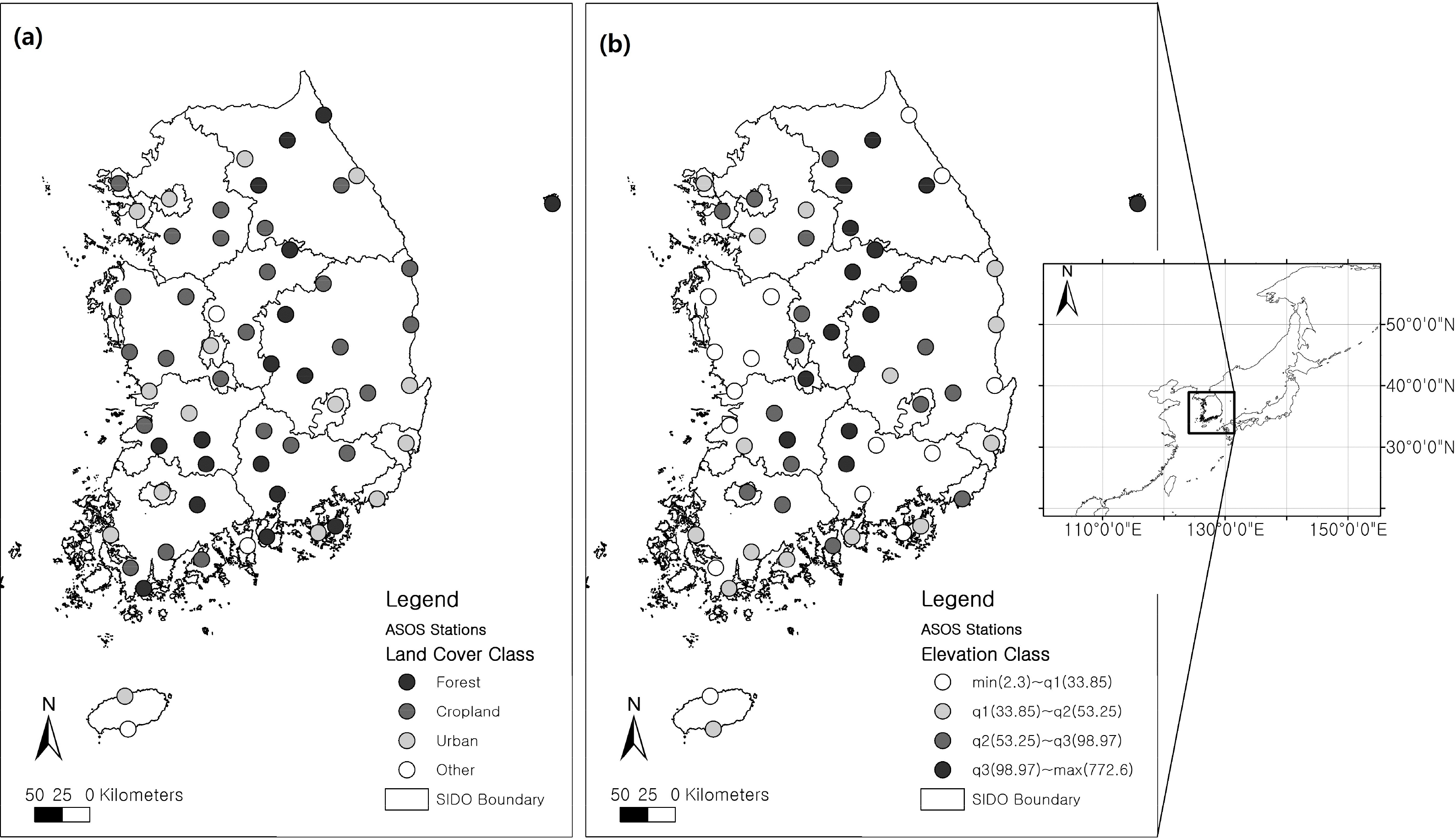
The study area of this study is South Korea, and sixty Automatic Synoptic Observation System (ASOS) weather stations located in South Korea (approximately within 124.3°E–131.3°E, 33°N–39°N) were used for analyses in this study (Figure 1). The study area experiences four distinct seasons over the course of the year and has complex topography with various land cover types. Such conditions allow the analysis of the effect of various factors, including seasonality, elevation, and land cover type, on air temperature estimation. Hourly temperature data are available for the 60 ASOS weather stations in the study area, which were used for the validation of the air temperature estimates.

2.2. Data

The Land Surface Temperature and Emissivity level-3 data products with daily (MYD11A1, Version 5) and eight-day (MYD11A2, Version 5) temporal resolutions and 1 × 1 km spatial resolution, as well as the Atmospheric Profile level-2 data product with 5-minute temporal resolution and 5 × 5 km spatial resolution (MYD07_L2, Version 5) from MODIS sensor onboard the Aqua satellite, were used to estimate daily and monthly air temperature in the study. The MYD11A2 eight-day data are the average of clear-sky values. The data were obtained from the Earth Observing System Data and Information System (EOSDIS) [18] of National Aeronautics and Space Administration (NASA), USA.

The MODIS Aqua data are available from July 2002, thus, all data from July 2002 to December 2011 were used in the study. The MYD11A1 and MYD11A2 data products include daytime and nighttime land surface temperature data, and the MYD07_L2 data product includes temperature and moisture data for 20 geopotential heights. The vertical temperature profile data are based on a regression algorithm with the Television Infrared Observation Satellite (TIROS) Operational Vertical Sounder (TOVS) data and derived using the International TOVS Processing Package (ITPP) [19,20]. Data from Aqua were used since the overpass times of the satellite are relatively closer to the times of daily maximum and minimum temperature. The air temperature data shift, based on a diurnal air temperature change model to overcome the time differences, was also examined in the following section.

Hourly, daily, and monthly, 2 m above ground level (AGL) air temperature data for the 60 ASOS weather stations were obtained from the Korea Meteorological Administration. Air temperature is measured at 2 m AGL as recommended by the World Meteorological Organization. The hourly data were used to examine the differences between the times of maximum and minimum air temperature and the times of solar noon and sunrise for use with the diurnal air temperature change model. The daily and monthly air temperature data were used to validate the estimated air temperature.

Two gridded datasets were used to test the correction of the air temperature estimates. The CRU TS3.20 dataset with monthly temporal resolution and 0.5° × 0.5° spatial resolution were obtained from the British Atmospheric Data Center (BADC) [21] and were used to correct the monthly air temperature estimates. The gridded NCEP/NCAR reanalysis data (Version 1), with daily temporal resolution and 2.5° × 2.5° spatial resolution, were obtained from the Physical Sciences Division (PSD) of the Earth System Research Laboratory of the National Oceanic and Atmospheric Administration (NOAA), USA, and used to correct the daily and monthly air temperature estimates.

Land cover type data from 2010 from MODIS (Terra and Aqua combined, MCD12Q1, Version 5) with a 500 × 500 m spatial resolution were obtained from EOSDIS. The dataset provides four types of land cover classifications; the International Geosphere-Biosphere Programme (IGBP) classification was used among them. Elevation was retrieved from the United States Geological Survey (USGS) Digital Elevation Model (DEM) GTOPO30 with 1 × 1 km spatial resolution. Land cover type and elevation data were used to examine their effect on the differences between the CRU dataset and the ASOS observation data, as well as on the monthly air temperature estimation.

3. Methodology

3.1. Data Processing

3.1.1. Land Surface Temperature Data

The daily daytime and nighttime land surface temperature data were obtained from the first and the fifth layers of the daily product (MYD11A1), respectively. The 8-day daytime and nighttime land surface temperature data were also obtained from the first and the fifth layers of the 8-day product (MYD11A2), respectively. The 8-day land surface temperature data are the composite of clear-sky days’ daily land surface temperature data. The daytime and nighttime, 8-day data were converted into monthly daytime and nighttime data using the number of days of each 8-day period as weights. Although the actual dates used for the composite can be obtained from metadata provided with data files, the information was not used to avoid such cases that the converted monthly data only represent a certain part of the month. The monthly daytime and nighttime land surface temperature values, as well as the daily daytime (descending) and nighttime (ascending) data (daytime LST and nighttime LST, hereafter) of the nearest pixels to the 60 ASOS weather stations were derived.

3.1.2. Vertical Temperature Profile Data

The Atmospheric Profile data include vertical moisture (Retrieved_Moisture_Profile) and temperature profile data (Retrieved_Temperature_Profile) for 20 geopotential heights (Retrieved_Height_Profile), from 5 hPa to 1000 hPa. Jocik [20] suggested a method to estimate 2 m AGL air temperature, based on a linear interpolation between the bottom profile level (1000 hPa) and ground level (2 m AGL). He used the pressure difference between 1000 hPa and 620 hPa levels, considering the vertical properties of the atmosphere, and calculated the ground level air temperature as the temperature of the 1000 hPa plus the adiabatic lapse rate, which resulted in a strong agreement with the observed data (R² = 0.84) for the study area [20].

In this study, a similar approach was applied and the 2 m AGL air temperature data were obtained, based on the linear interpolation/extrapolation, using the geopotential height and air temperature data of 620 hPa and 1000 hPa and the GTOPO30 elevation. The linear relationship between the geopotential height and air temperature in the lower levels is assumed in Equation (1), where T is air temperature and z is geopotential height. Slope a and intercept b may be obtained using data at 620 hPa and 1000 hPa levels (Equations (2) and (3)), where T_{1000 hPa}, T_{620 hPa}, z_{1000 hPa}, and z_{620 hPa} are air temperature at 1000 hPa level, air temperature at 620 hPa level, geopotential height at 1000 hPa level, and geopotential height at 620 hPa level, respectively. The 2 m AGL air temperature can then be calculated using the height above mean sea level (AMSL), which is elevation AMSL plus 2 meters.

$$T=a\cdot z+b$$

(1)

$$a=\frac{T_{1000\mathit{hPa}}-T_{620\mathit{hPa}}}{z_{1000\mathit{hPa}}-z_{620\mathit{hPa}}}$$

(2)

$$b=T_{1000\mathit{hPa}}-z_{1000\mathit{hPa}}\cdot a$$

(3)

For missing 1000 hPa level data, 950 hPa level data were used instead. Linear regression was also tested but showed little difference to linear interpolation/extrapolation. Since the Atmospheric Profile (AP) data are obtained with 5-min temporal resolution, the MODIS overpasses each location about 2 to 5 times a day. The 2 m AGL air temperature estimates were averaged for each day but for daytime and nighttime separately. The data were also converted to monthly, and the daily and monthly daytime and nighttime 2 m AGL air temperature estimates (daytime AP and nighttime AP, hereafter) of the nearest pixels to the 60 ASOS weather stations were then derived.

3.2. Diurnal Air Temperature Change Model

The local equatorial crossing time of the Aqua satellite is about 1:30 p.m. in an ascending mode and about 1:30 a.m. in a descending mode. The overpass time over the study area is about the same local time. Since the daily air temperature reaches its maximum about a couple of hours after solar noon, and reaches its minimum just before [22] or after [23] sunrise, there exist time gaps between the times for daily maximum and minimum air temperature and the MODIS overpass times. In this study, a diurnal air temperature change model was proposed to estimate the maximum and minimum air temperature using the daytime and nighttime AP and the MODIS overpass times.

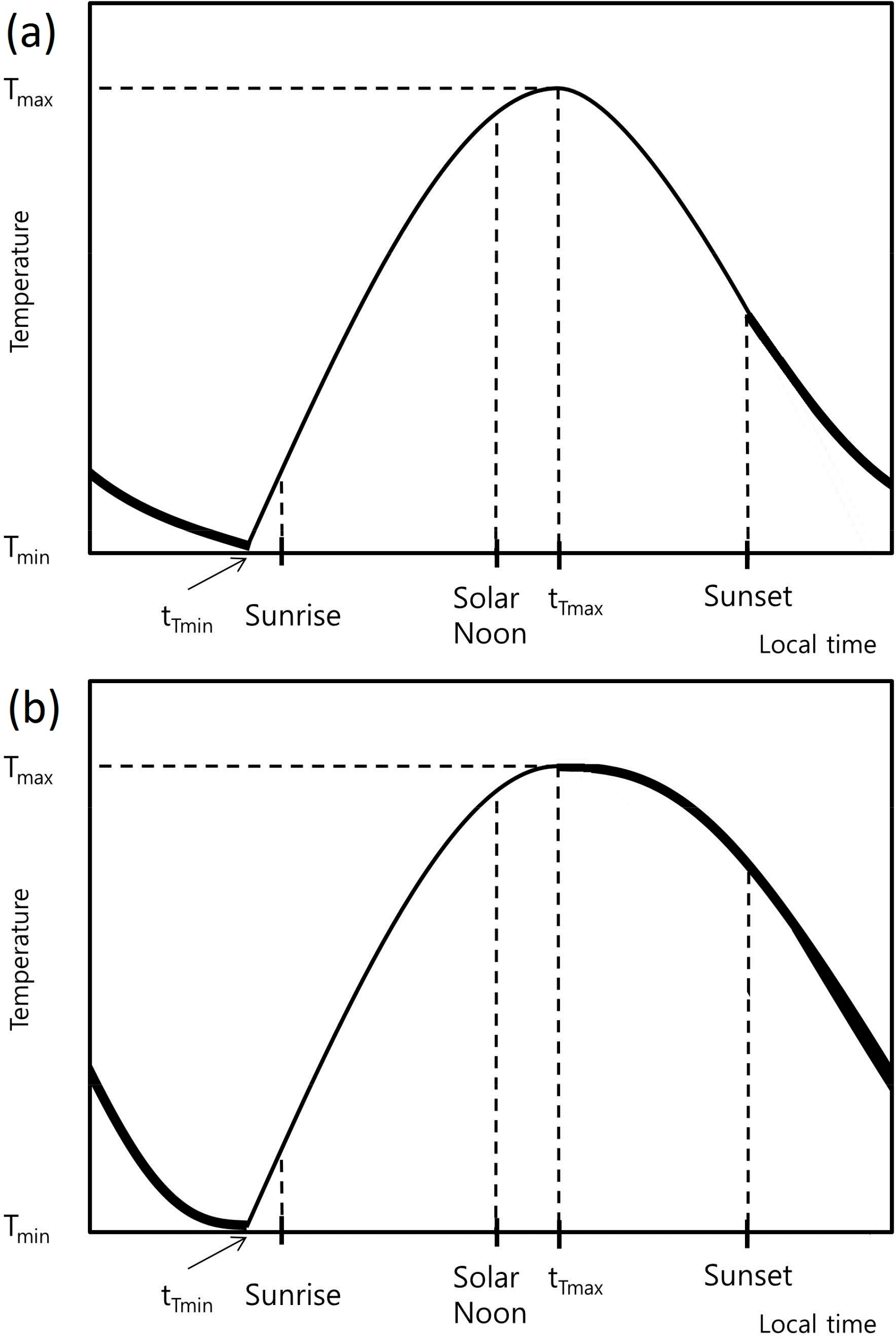
Lagouarde and Brunet [22] proposed a diurnal surface temperature change model with part of a sine function during the day, and part of a parabola during the night. Parton and Logan [24] proposed a diurnal air temperature change model using part of a sine function during the day and part of an exponential function during the night. A model with sine and exponential functions was initially considered in this study, but it requires the time between maximum and minimum air temperatures being longer than the time between sunset and maximum temperature (Figure 2a). A model with two sine functions for ascending and descending temperatures was proposed (Figure 2b) and it produces similar results with the model that uses sine and exponential functions, while representing the generally slowly decreasing air temperature after reaching maximum temperature [23].

Sunrise, sunset, and solar noon times for each day were calculated for each of the 60 ASOS weather stations using astronomical algorithms in the pyephem library of Python, and used, as is, for daily analysis or averaged for each month for monthly analysis. The times for maximum and minimum air temperatures were derived as functions of sunrise and solar noon times, based on the data from the weather stations to be used with the proposed diurnal air temperature change model (Equations (4) and (5)).

$$t_{T_{\mathit{min}}}=t_{T_{\mathit{rise}}}-1$$

(4)

$$t_{T_{\mathit{max}}}=t_{T_{\mathit{noon}}}+2$$

(5)

where T is temperature and t is local time; thus t_Tmin, t_Trise, t_Tmax, t_Tnoon are local times for daily minimum temperature, sunrise, daily maximum temperature, and solar noon, respectively. Using the following equations representing air temperature, based on two sine functions for ascending and descending temperatures proposed in this study (Equations (6) to (8)), daily and monthly daytime and nighttime APs can be shifted to daily and monthly maximum and minimum temperatures, respectively (AP_shift, hereafter). As there were little seasonal differences observed in the shape of the diurnal air temperature change when analyzed with hourly air temperature data, the same type of model could be used for all months, only with different amplitudes and frequencies of sine functions.

$$\text{T}=\left(T_{\mathit{max}}-T_{\mathit{min}}\right)\text{sin}\left\{\frac{\pi }{2}\frac{\left(t-t_{T_{\mathit{min}}}\right)}{\left(t_{T_{\mathit{max}}}-t_{T_{\mathit{min}}}\right)}\right\}+T_{\mathit{min}},t_{T_{\mathit{min}}}\le \text{t}<t_{T_{\mathit{max}}}$$

(6)

$$\text{T}=-\left(\frac{T_{\mathit{max}}-T_{\mathit{min}}}{2}\right)\text{sin}\left\{\frac{\pi \left(t-\frac{t_{T_{\mathit{max}}}+t_{T_{\mathit{min}}}-24}{2}\right)}{t_{T_{\mathit{min}}}-t_{T_{\mathit{max}}}+24}\right\}+\left(\frac{T_{\mathit{max}}+T_{\mathit{min}}}{2}\right),0<t\le {\text{t}}_{T_{\mathit{min}}}$$

(7)

$$\text{T}=-\left(\frac{T_{\mathit{max}}-T_{\mathit{min}}}{2}\right)\text{sin}\left\{\frac{\pi \left(t-\frac{t_{T_{\mathit{max}}}+t_{T_{\mathit{min}}}+24}{2}\right)}{\left(t_{T_{\mathit{min}}}-t_{T_{\mathit{max}}}+24\right)}\right\}+\left(\frac{T_{\mathit{max}}+T_{\mathit{min}}}{2}\right),\text{t}\ge {\text{t}}_{T_{\mathit{max}}}$$

(8)

3.3. Correction Using Gridded Datasets

The correction of the estimated air temperature using gridded climate datasets by fitting linear regression models (Equation (9)) for each ASOS location was tested to examine the possible improvements.

$$\mathit{Corrected}\hspace{0.17em}\mathit{Estimates}=\mathit{Uncorrected}\hspace{0.17em}\mathit{Estimates}\times \text{c}+\text{d}$$

(9)

In Equation (9), the coefficients c and d indicate slope and intercept of the regression model. The CRU dataset was selected for correcting monthly estimates since it includes monthly maximum and minimum air temperature and it is available over the globe. The NCEP/NCAR reanalysis dataset was selected for correcting daily and monthly estimates since it has daily maximum and minimum air temperature, and it is also available all over the globe.

3.4. ANOVA for Land Cover and Elevation

The 60 ASOS weather stations’ locations include six IGBP land cover classes; similar classes were grouped together to create three distinct classes of Forest (17 stations with Evergreen needle leaf forest and Mixed forest land cover types), Cropland (25 stations with Grasslands, Croplands, and Cropland/Natural vegetation mosaic land cover types), and Urban (15 stations with Urban and built-up land cover type, Figure 1). The remaining three stations, with majority land cover type of Water, Permanent wetlands, and Open shrublands (Other land cover type in Figure 1), were not included in the analysis. Quartiles of the elevation data of the 60 ASOS weather stations were calculated and the weather stations were grouped into four elevation classes: CL1 (from minimum elevation = 2.3 m to Q1 = 33.85 m), CL2 (from Q1 to Q2 = 53.25 m), CL3 (from Q2 to Q3 = 98.94 m), and CL4 (from Q3 to maximum = 772.6 m, Figure 1).

One-way Analysis of Variance (ANOVA) tests were performed to examine the effect of land cover and elevation classifications, respectively, on the differences between the CRU dataset and the ASOS observation data, as well as on the estimation of air temperature. Null hypotheses are that there is no difference in the estimated air temperature between land cover classes and between elevation classes, respectively.

4. Results and Discussion

4.1. Maximum and Minimum Air Temperature Estimation

Observation data from the 60 ASOS weather stations were used to validate the estimated air temperature from LST and AP. Although the grid data represent the average of an area and the weather station data represent a point, the comparisons between the 60 ASOS weather stations’ locations and the nearest pixels to the stations were made as the gridded data could be considered the best estimates for regions without observation data for any location of interests. Coefficient of determination (R²) values show how much variance of the predictand can be explained by the predictor. For daily estimation, AP showed a better agreement with observation data than LST in spring (March, April, and May; MAM) and summer (June, July, and August; JJA) for maximum temperature, and in all seasons for minimum temperature (

Table 1. Coefficient of determination (R²) values averaged for 60 Automatic Synoptic Observation System (ASOS) weather stations’ locations for estimating daily and monthly air temperature (unitless).

Variable	Season	Daily Estimation			Monthly Estimation
		AP	AP_Shift	LST	AP	AP_Shift	LST
Maximum Temperature	ALL	0.87	0.87	0.84	0.95	0.95	0.94
	MAM	0.77*	0.76	0.75	0.89	0.89	0.93
	JJA	0.64	0.63	0.28	0.41	0.43	0.12
	SON	0.84	0.84	0.89	0.92	0.92	0.96
	DJF	0.67	0.67	0.74	0.62	0.57	0.72
Minimum Temperature	ALL	0.92	0.92	0.87	0.94	0.94	0.97
	MAM	0.85	0.85	0.71	0.89	0.89	0.96
	JJA	0.83	0.82	0.65	0.77	0.76	0.75
	SON	0.90	0.89	0.81	0.92	0.91	0.95
	DJF	0.57	0.57	0.45	0.35	0.30	0.52

^*Values in bold indicate high coefficient values.

). In autumn (September, October, and November; SON) and winter (December, January, and February; DJF), LST produced slightly higher R² values for maximum temperature (Table 1). For monthly estimation, LST outperformed AP in all seasons except during JJA (Table 1). The R² values during MAM and SON were very high; daytime LST explains 93% of variance of monthly maximum air temperature during MAM and 96% during SON. On the other hand, the R² values were quite low during DJF and, especially, JJA; LST explains only 12% of variance of monthly maximum air temperature during JJA. AP showed better performance than LST; it explains 41% of variance for the same season (Table 1).

When the performance of daily LST was compared with that of monthly LST, the latter showed higher R² values than the former for both maximum and minimum temperature in most seasons. It is possibly due to larger temperature variations of daily LST than monthly LST. Similarly, the poor estimation of maximum air temperature by monthly LST during JJA may be explained by the large variation of maximum air temperature, resulting in the monthly averaging being inappropriate. The R² values of daily and monthly LST during JJA were especially low, indicating the high usability of daily and monthly APs that resulted in much higher R² values.

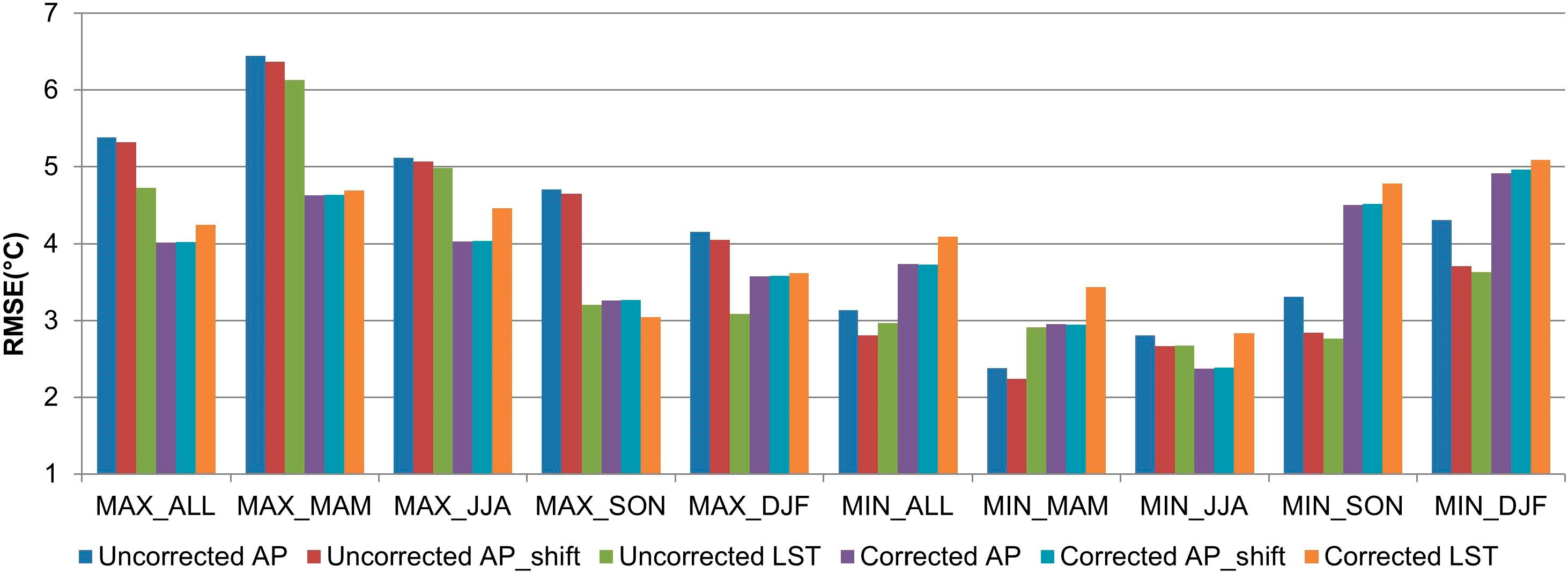
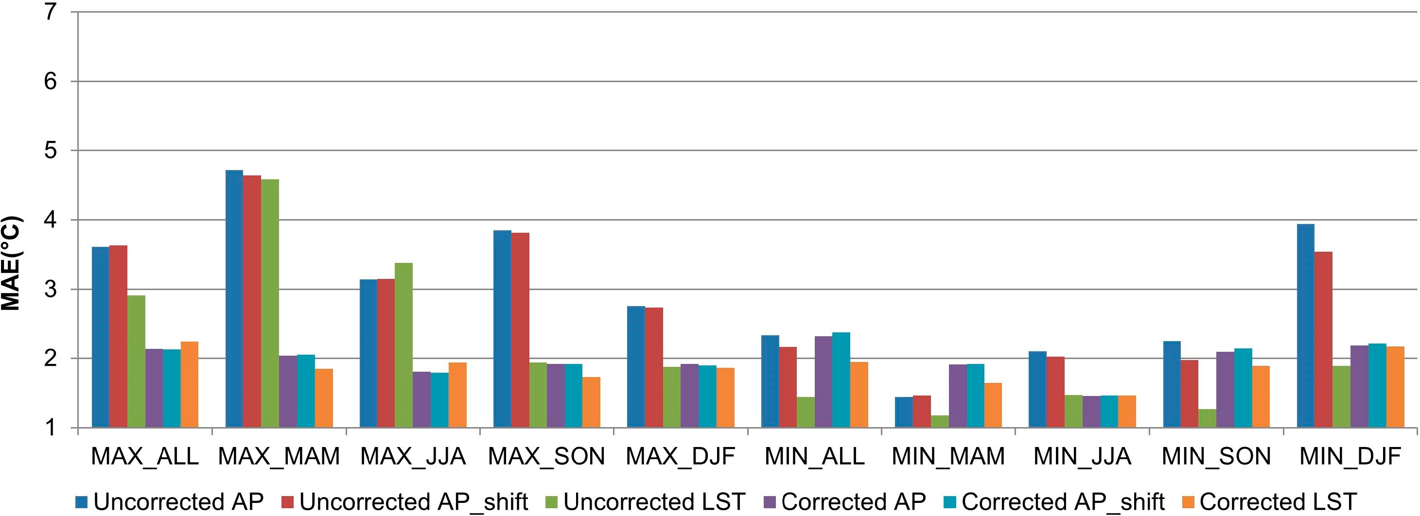
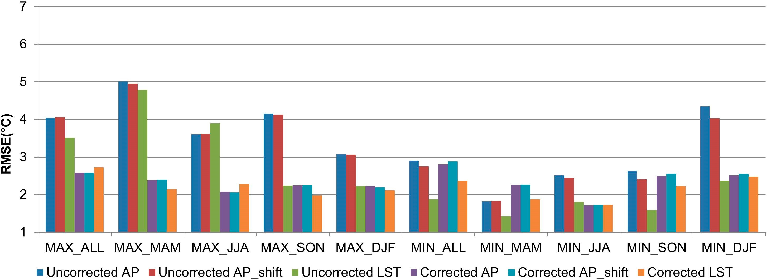
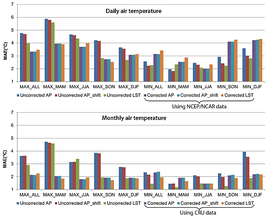
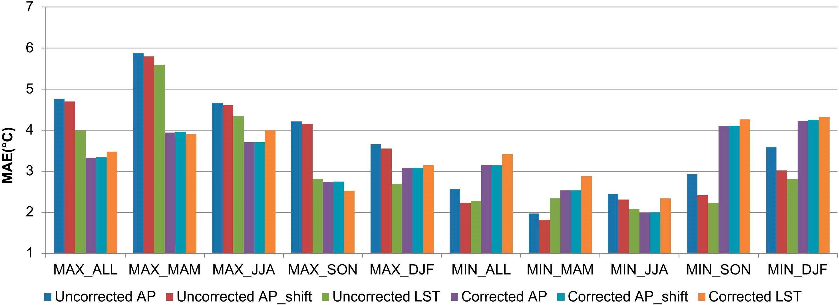
Since the purpose of the study is to estimate daily and monthly air temperature for regions with limited in situ data, the estimates are supposed to be used without observation data. In this case, the error values, such as MAE and RMSE, become very important criteria. The MAE and RMSE values of LST and AP were calculated for daily (Figures 3 and 4) and monthly estimations (Figures 5 and 8). Uncorrected LST produced smaller MAE and RMSE than AP in all seasons for both daily maximum and minimum temperature, except during MAM for daily minimum temperature and during JJA for monthly maximum temperature (Figures 3 and 6).

4.2. Data Shift Based on the Diurnal Air Temperature Change Model

The coefficient of determination values of uncorrected AP_shift were slightly higher only during JJA for monthly maximum air temperature compared to AP, while the values were slightly lower or the same in other cases (Table 1). The MAE and RMSE values of uncorrected AP_shift were somewhat smaller than AP in all seasons for daily maximum air temperature, and during MAM, SON, and DJF for monthly maximum air temperature (Figures 3 and 6). Larger differences were observed for minimum air temperature; uncorrected AP_shift showed smaller MAE and RMSE than AP in all seasons for daily minimum air temperature, and during JJA, SON, and DJF, for monthly minimum air temperature (Figures 3 and 6). The improvements from the shift were not large for maximum air temperature because the MODIS overpass time, in an ascending mode, is quite close to the time that the air temperature reaches its maximum. On the other hand, the MODIS overpass time in a descending mode (about 1:30 a.m.) is quite apart from the time the air temperature reaches its minimum (about one hour before sunrise), thus, the improvements by the data shift were more obvious. However, the error values of AP_shift are larger than those of LST for both maximum and minimum temperatures in most seasons, except during MAM (and also during JJA for RMSE) for daily minimum temperature and during JJA for monthly maximum temperature (Figures 5 and 8).

4.3. Correction Using the Gridded Datasets

The correction using the gridded datasets did not affect the coefficient of determination values because the correction was based on a linear transformation, as shown in Equation (9), while the MAE and RMSE values were significantly reduced (Figures 3 and 8). When daily air temperature estimates were corrected using the NCEP/NCAR reanalysis data, MAE and RMSE values were reduced in all seasons for daily maximum air temperature (Figures 3 and 4, ΔMAE = −0.28 to −1.93, ΔRMSE = −0.16 to −1.82), except LST during DJF. For daily minimum air temperature, MAE and RMSE were improved only for AP and AP_shift during JJA. The correction of LST using the gridded datasets improved the estimation of maximum temperature better than minimum temperature, because surface temperature is known to be higher than air temperature during the day, while it is close to air temperature during the night [11,13]. The difference between surface temperature and air temperature depends on a complex surface energy balance during the day, but the effect of solar radiation is minor during the night [13].

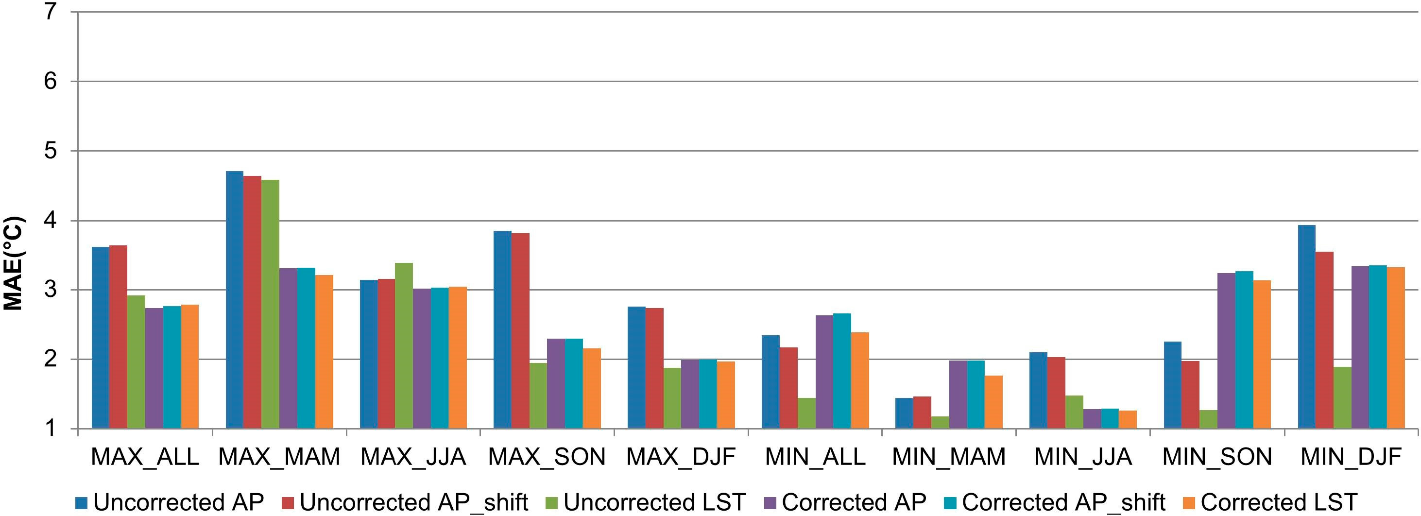
The MAE and RMSE values also decreased in all seasons when monthly maximum air temperature was corrected using the CRU dataset (Figures 5 and 6, ΔMAE = −0.01 to −2.73, ΔRMSE = −0.11 to −2.66). For monthly minimum air temperature, the error values of AP decreased during JJA, SON, and DJF (Figures 5 and 6; ΔMAE = −0.16 to −1.75, ΔRMSE = −0.14 to −1.84) when corrected using the CRU dataset, and the error values of AP_shift decreased during JJA and DJF (Figures 5 and 6; ΔMAE = −0.56 to −1.33, ΔRMSE = −0.72 to −1.48). The LST showed reduced error values during JJA (Figures 5 and 6, ΔMAE = −0.01, ΔRMSE = −0.09).

The decrease of MAE and RMSE values of monthly maximum air temperature was larger when corrected using the CRU dataset compared to the NCEP/NCAR reanalysis dataset (Figures 5 and 8). The MAE and RMSE of daily and monthly air temperature after the correction using the NCEP/NCAR reanalysis dataset remained quite large, compared to results from existing studies, due to the coarse spatial resolution of the dataset.

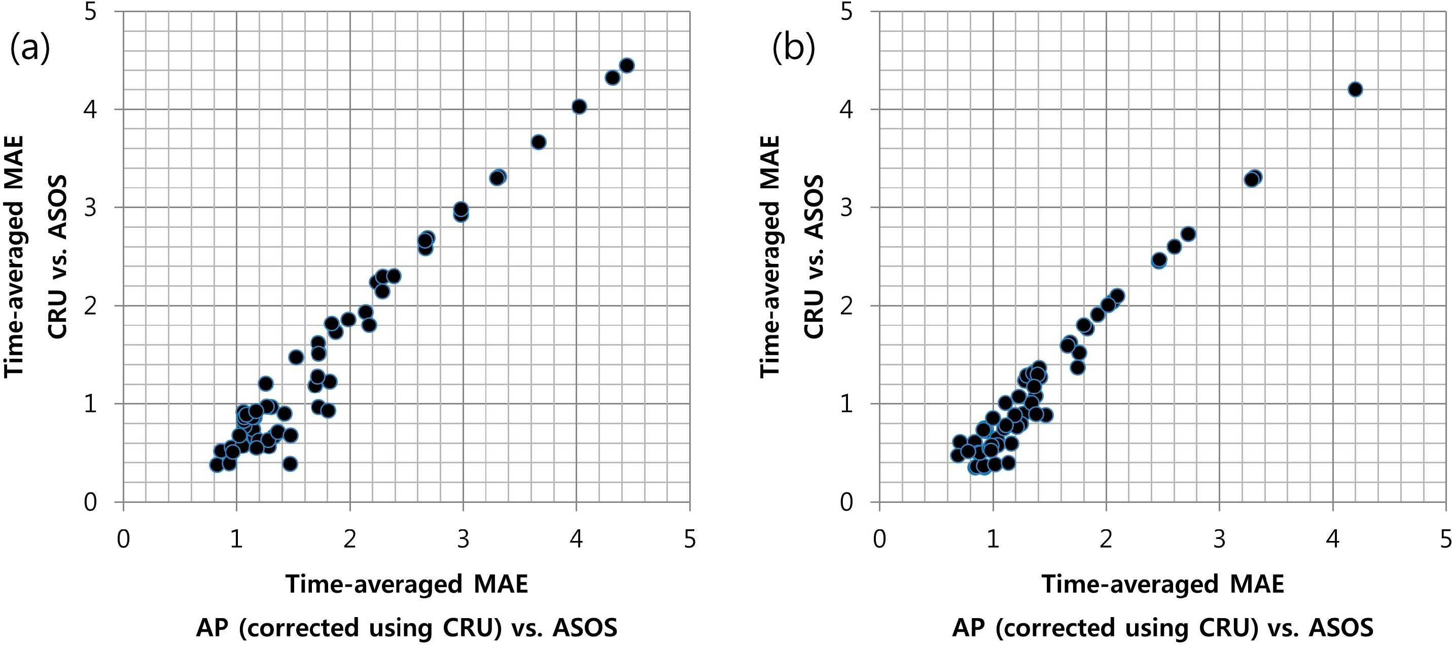
Although the errors were generally reduced thanks to the correction using the gridded datasets especially for maximum air temperature, the correction introduced a new source of error. The MAE and RMSE values for each ASOS weather station’s location were examined and it was found that the stations with relatively large errors were the same stations with larger differences between the ASOS observation data and the gridded dataset (Figure 9 with CRU data), implying that the discrepancy between the ASOS observation data and the gridded dataset is the new source of error. The discrepancy may be larger if applied for regions with limited in situ data compared to the study area where a moderately dense observation network exists, which must have improved the quality of the gridded dataset for the area. However, the correction using the gridded dataset especially the CRU, helped error values to decrease for many stations as previously mentioned.

4.4. Effect of Land Cover and Elevation

Results of the correction of the estimated monthly air temperature using the CRU dataset, which produced the smallest error values, indicated that five ASOS weather stations showed especially large differences between the CRU dataset and ASOS observation data (MAE of maximum and minimum air temperature > 3.0 °C for all seasons); although they were located in the southern part of the study area (not shown), there was no common distinct characteristic found, such as the distance from shoreline, land cover type, and elevation.

One-way ANOVA tests were performed to see the differences in error values due to different land cover and elevation classes, respectively. For both maximum and minimum air temperature, no difference between land cover and elevation classes was observed in the error values between the CRU dataset and ASOS observation data, and the null hypotheses could not be rejected (

Table 2. Test statistics for one-way ANOVA testing differences between land cover classes of Mean Absolute Error (MAE) values between ASOS observation data vs. the Climate Research Unit (CRU) dataset and monthly air temperature estimates with or without the correction using the CRU data. Values in bold indicate that there is a significant difference at the 95% confidence level.

Variable	Season	CRU Dataset	Uncorrected		Corrected
			AP	LST	AP	LST
Maximum Temperature	ALL	0.15	0.03	<0.0001	0.14	0.16
	MAM	0.13	0.06	0.0001	0.06	0.14
	JJA	0.12	0.003	<0.0001	0.16	0.34
	SON	0.12	0.02	<0001	0.10	0.12
	DJF	0.40	0.13	0.06	0.50	0.39
Minimum Temperature	ALL	0.07	<0.0001	0.68	0.34	0.16
	MAM	0.06	0.09	0.37	0.05	0.04
	JJA	0.07	0.0005	0.62	0.09	0.23
	SON	0.11	0.001	0.91	0.43	0.19
	DJF	0.13	<0.0001	0.12	0.21	0.36

and

Table 3. Test statistics for one-way ANOVA testing differences between elevation classes of MAE values between ASOS observation data vs. the CRU dataset and monthly air temperature estimates with or without the correction using the CRU data. Values in bold indicate that there is a significant difference at the 95% confidence level.

Variable	Season	CRU Dataset	Uncorrected		Corrected
			AP	LST	AP	LST
Maximum Temperature	ALL	0.33	0.06	0.03	0.34	0.34
	MAM	0.12	0.06	0.03	0.12	0.15
	JJA	0.24	0.13	0.04	0.44	0.71
	SON	0.36	0.07	0.10	0.32	0.42
	DJF	0.78	0.12	0.36	0.84	0.81
Minimum Temperature	ALL	0.67	0.03	0.26	0.91	0.83
	MAM	0.73	0.42	0.35	0.85	0.75
	JJA	0.60	0.0006	0.10	0.74	0.67
	SON	0.31	0.05	0.47	0.53	0.45
	DJF	0.62	0.04	0.28	0.83	0.74

). The discrepancy between the CRU dataset and the ASOS weather station data may be due to the coarse spatial resolution of the CRU dataset.

Estimation errors of air temperature from AP and LST varied by land cover and elevation classes: differences were observed between land cover classes for uncorrected LST during MAM, JJA, and SON, when estimating maximum air temperature and also for uncorrected AP during JJA and SON (null hypothesis rejected with significance level of 0.05). When estimating minimum air temperature, differences were observed for uncorrected AP during JJA, SON, and DJF (Table 2). Such differences were not observed for corrected LST and AP, except during MAM when estimating minimum air temperature (Table 2).

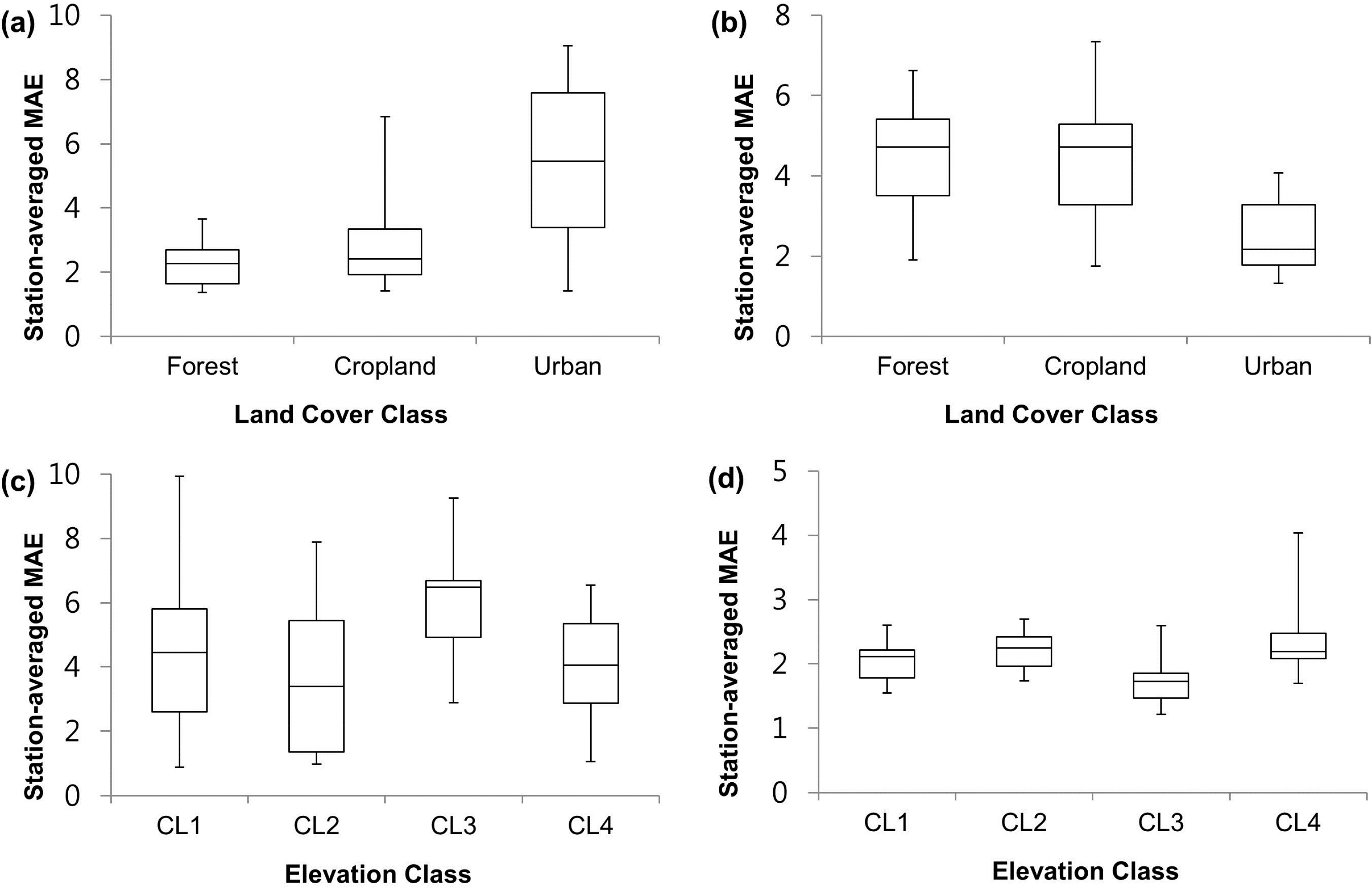
The station-averaged MAE values between different land cover classes were examined for uncorrected LST during JJA (Figure 10a) and uncorrected AP during DJF (Figure 10b). The major differences appear in urban areas; the averaged error value was larger in stations with the urban land cover class for uncorrected LST while it was smaller for uncorrected AP (Figure 10a,b). The larger error of uncorrected LST in urban areas for estimating air temperature is due to the high percentage of impervious areas, which exacerbate the discrepancy between the surface and air temperature, especially during the day. The urban areas are also affected by the urban heat island effect, which increases the air temperature especially during the night. It is likely that the error values between uncorrected AP and ASOS observation data are smaller in urban areas due to the increased air temperature caused by the heat island effect, leading to better estimation of 2 m AGL air temperature from the vertical temperature profile data.

For elevation classes, the null hypothesis could be rejected for uncorrected LST during MAM and JJA when estimating maximum air temperature and for uncorrected AP during JJA, SON, and DJF, when estimating minimum air temperature implying differences in error values between elevation classes (Table 3). However, no increasing or decreasing trend of errors with elevation was observed (Figure 10c,d). Such differences were also not observed for corrected LST and AP (Table 3).

5. Conclusions

Both land surface temperature and vertical temperature profile data could be successfully used to estimate the 2 m AGL daily and monthly maximum and minimum air temperature in most seasons. They showed quite large coefficient of determination values and produced relatively smaller or comparable errors to existing studies, even though observation data from the weather stations were not used for the estimation. Daily and monthly LST outperformed AP in most seasons for both maximum and minimum temperature in terms of error values, but AP showed much higher coefficient of determination values during JJA. AP_shift based on the diurnal air temperature change model improved the estimation by producing smaller error values in most cases, but LST still outperformed AP_shift in most seasons for both maximum and minimum air temperatures.

Corrections based on gridded datasets improved the estimation, especially for maximum air temperature. The use of the NCEP/NCAR reanalysis data for the correction, however, still produced somewhat large error values despite the significant decrease of the error values. When corrected using the CRU dataset, the MAE values for estimating monthly maximum air temperature range from 1.73 °C to 1.86 °C (AP or AP_shift for JJA, and LST for other seasons). Uncorrected LST generally performed better for estimating monthly minimum air temperature and the MAE values range from 1.18 °C to 1.89 °C. The spatial resolutions of the estimates are 1 × 1 km for LST and 5 × 5 km for AP and AP_shift.

A methodology for creating high spatial resolution air temperature data for regions with limited in situ data was developed in this study. It can be used for many environmental and agricultural studies requiring air temperature data at the daily or monthly resolution. The error values of daily air temperature estimates using LST and AP were slightly larger compared to monthly estimates. Although the correction using the gridded dataset for estimating maximum air temperature may introduce a different source of error, the discrepancy between the gridded dataset and the observation data, the correction still can improve the estimation considerably even for daily air temperature. Such a discrepancy, possibly due to the coarse spatial resolution of the gridded dataset, typically increases uncertainties in estimating maximum and minimum temperatures especially at the daily temporal resolution. In order to reduce uncertainties and errors associated with the performance of LST and AP for estimating daily or monthly maximum and minimum temperatures, finer resolution gridded climate datasets, such as the Asian Precipitation Highly Resolved Observational Data Integration Towards Evaluation (APHRODITE) dataset for the Asia region, can be used. The use of NCEP/NCAR reanalysis data produced rather large error values due to its coarser spatial resolution.

For estimating maximum air temperature, it may be generally recommended to use corrected LST during MAM and SON (also during DJF with monthly data) and to consider AP or AP_shift during JJA. For minimum air temperature, uncorrected LST during SON and DJF (also during MAM with monthly data), and corrected AP or AP_shift during JJA may be used.

There are some limitations to be resolved in further studies. In order to use the diurnal air temperature change model, the times for maximum and minimum air temperature were derived as functions of solar noon and sunrise based on the observation data, which needs more case studies. The air temperature for cloudy days and the effect of soil moisture on air temperature should be considered in further studies. Remotely sensed data based on microwave sensors may resolve the issues, and will also ease the estimation of daily air temperature. Although the study area is located in a temperate climate region, the findings may be applied in many data sparse areas since the study area has complex topography and a wide range of temperature over the course of the year.

References

- Hargreaves, G.L.; Hargreaves, G.H.; Riley, J. Agricultural benefits for Senegal River basin. J. Irrig. Drain. Eng 1985, 111, 113–124. [Google Scholar]
- Allen, R.; Pereira, L.; Raes, D.; Smith, M. Crop Evapotranspiration—Guidelines for Computing Crop Water Requirements; FAO Irrigation and Drainage Paper 56; Food and Agriculture Organization of the United Nations: Rome, Italy, 1998; p. 300. [Google Scholar]
- Cuba, N.; Rogan, J.; Christman, Z.; Williams, C.; Schneider, L.; Lawrence, D.; Millones, M. Modelling dry season deciduousness in Mexican Yucatan forest using MODIS EVI data (2000–2011). GISci. Remote Sens 2013, 50, 26–49. [Google Scholar]
- Lu, J.; Tang, R.; Tang, H.; Li, Z. Derivation of daily evaporative fraction based on temporal variations in surface temperature, air temperature, and net radiation. Remote Sens 2013, 5, 5369–5396. [Google Scholar]
- Zhang, Y.; Hepner, G.; Dennison, P. Delineation of phenoregions in geographically diverse regions using k-means++ clustering: A case study in the upper Colorado River basin. GISci. Remote Sens 2012, 49, 163–181. [Google Scholar]
- Cooke, W.; Mostovoy, G.; Anantharal, V.; Jolly, W. Wildfire potential mapping over the State of Mississippi: A land surface modeling approach. GISci. Remote Sens 2012, 49, 492–509. [Google Scholar]
- Lawrimore, J.; Menne, M.; Gleason, B.; Williams, C.; Wuertz, D.; Vose, R.; Rennie, J. An overview of the Global Historical Climatology Network monthly mean temperature data set, version 3. J. Geophys. Res 2011. [Google Scholar] [CrossRef]
- Daly, C.; Neilson, R.; Phillips, D. A statistical-topographic model for mapping climatological precipitation over mountainous terrain. J. Appl. Meteor 1994, 33, 140–158. [Google Scholar]
- Hill, D. An assessment of spatial models for daily minimum and maximum air temperature. GISci. Remote Sens 2013, 50, 281–300. [Google Scholar]
- Prihodko, L.; Goward, S. Estimation of air temperature from remotely sensed surface observations. Remote Sens. Environ 1997, 60, 335–346. [Google Scholar]
- Jang, J.; Viau, A.; Anctil, F. Neural network estimation of air temperatures from AVHRR data. Int. J. Remote Sens 2004, 25, 4541–4554. [Google Scholar]
- Yan, H.; Zhang, J.; Hou, Y.; He, Y. Estimation of air temperature from MODIS data in east China. Int. J. Remote Sens 2009, 30, 6261–6275. [Google Scholar]
- Lin, S.; Moore, N.; Messina, J.; DeVisser, M.; Wu, J. Evaluation of estimating daily maximum and minimum air temperature with MODIS data in East Africa. Int. J. Appl. Earth Obs 2012, 18, 128–140. [Google Scholar]
- Williamson, S.; Hik, D.; Gamon, J.; Kavanaugh, J.; Flowers, G. Estimating temperature fields from MODIS land surface temperature and air temperature observations in a sub-arctic alpine environment. Remote Sens 2013, 6, 946–963. [Google Scholar]
- Vancutsem, C.; Ceccato, P.; Dinku, T.; Connor, S. Evaluation of MODIS land surface temperature data to estimate air temperature in different ecosystems over Africa. Remote Sens. Environ 2010, 114, 449–465. [Google Scholar]
- Benali, A.; Carvalho, A.; Nunes, J.; Carvalhais, N.; Santos, A. Estimating air surface temperature in Portugal using MODIS LST data. Remote Sens. Environ 2012, 124, 108–121. [Google Scholar]
- Miliaresis, G.; Tsatsaris, A. Mapping the spatial and temporal pattern of day-night temperature difference in Greece from MODIS imagery. GISci. Remote Sens 2011, 48, 210–224. [Google Scholar]
- Earth Observing System Data and Information System (EOSDIS). Available online: http://reverb.echo.nasa.gov (accessed on 22 April 2013).
- Borbas, E.; Seemann, S.; Kern, A.; Moy, L.; Li, J.; Gumley, L.; Menzel, W. MODIS Atmospheric Profile Retrieval Algorithm Theoretical Basis Document, Collection 6; Cooperative Institute for Meteorological Satellite Studies, University of Wisconsin-Madison: Madison, WI, USA, 2011; p. 30. [Google Scholar]
- Mendez Jocik, A. Estimate Ambient Air Temperature at Regional Level Using Remote Sensing Techniques. Master’s Thesis. Sustainable Agriculture Specialization, International Institute for Geo-Information Science and Earth Observation, Enschede, The Netherlands, 2004; p. 86. [Google Scholar]
- Jones, I.H. CRU TS3.20: Climatic Research Unit (CRU) Time-Series (TS) Version 3.20 of High Resolution Gridded Data of Month-by-Month Variation in Climate (January 1901–December 2011). Available online: http://badc.nerc.ac.uk/view/badc.nerc.ac.uk__ATOM__ACTIVITY_3ec0d1c6-4616-11e2-89a3-00163e251233 (accessed on 18 November 2013).
- Lagouarde, J.; Brunet, Y. A simple model for estimating the daily upward longwave surface radiation flux from NOAA-AVHRR data. Int. J. Remote Sens 1993, 14, 907–925. [Google Scholar]
- Aguado, E.; Burt, J. Understanding Weather and Climate, 4th ed.; Pearson Prentice Hall: Upper Saddle River, NJ, USA, 2007; p. 562. [Google Scholar]
- Parton, W.; Logan, J. A model for diurnal variation in soil and air temperature. Agr. Meteor 1981, 23, 205–216. [Google Scholar]