The Use of a Hand-Held Camera for Individual Tree 3D Mapping in Forest Sample Plots

Abstract

This paper evaluated the feasibility of a terrestrial point cloud generated utilizing an uncalibrated hand-held consumer camera at a plot level and measuring the plot at an individual-tree level. Individual tree stems in the plot were detected and modeled from the image-based point cloud, and the diameter-at-breast-height (DBH) of each tree was estimated. The detected-results were compared with field measurements and with those derived from the single-scan terrestrial laser scanning (TLS) data. The experiment showed that the mapping accuracy was 88% and the root mean squared error of DBH estimates of individual trees was 2.39 cm, which is acceptable for practical applications and was similar to the results achieved using TLS. The main advantages of the image-based point cloud data lie in the low cost of the equipment required for the data collection, the simple and fast field measurements and the automated data processing, which may be interesting and important for certain applications, such as field inventories by landowners who do not have supports from external experts. The disadvantages of the image-based point cloud data include the limited capability of mapping small trees and complex forest stands.

1. Introduction

Reference data collected from sample plots are fundamental for forest inventory and ecology. Plot- and individual-tree-level measurements are made in sample plots. Plot-level measurement takes a sample plot as a minimum unit and describes the plot using average values, whereas individual-tree-level measurement collects the attributes of each tree. The latter has the advantage of providing more accurate and comprehensive information regarding a sample plot. If tree locations were also measured, individual trees in the sample plots can be connected to high-resolution remote sensing (RS) data, which can be then utilized to teach RS data to carry out precision forest inventories over large areas. However, plot-level measurement is commonly utilized in practice due to its simplicity and cost effectiveness.

The difficulty of individual-tree-level plot measurements is mainly raised from the lack of effective measurement solutions, especially for mapping tree locations in sample plots. Conventionally, the locations of individual trees in a plot are measured using devices such as a rangefinder and a bearing compass. Other relevant tree attributes are acquired by using specific instruments, e.g., dendrometers and relascopes. New instruments are constantly being developed: a laser relascope has been developed to measure stem locations relative to the plot center and the diameter at breast height (DBH); and a system based on the Postex and Digitech Professional caliper (Haglöf Sweden AB, Långsele, Sweden) provides the tree locations, DBHs and heights in the plot by accessing individual trees. However, all these solutions are built on manual measurements; hence, they are still time consuming and labor intensive.

Several studies attempted to automate the tree measurement by using terrestrial images. An imaging system was developed in [1] and consisted of a calibrated camera, a laser distance measurement device and a calibration stick. By using a tapering model for the image interpretation, the stem curves of Scots pines can be estimated. A laser-camera that was developed in [2] integrated a digital camera and a laser line generator to measure the DBH of individual trees. In the reported experiment, the automated diameter measurement detected 57.4% of valid observations. The standard deviation of the measurable observations was 1.27 cm. A 360° panorama plot image was used in [3] to produce a stem map. Field-measured DBHs and image-derived DBHs were jointly employed for the calculation of the location of trees in the plot; 85% of the measured trees were within 0.5 m of the field-measured tree location. With these methods, the automation level is increased compared with manually measuring individual trees utilizing conventional tools. However, substantial manual work is still required. This actually indicates the difficulty of automated individual tree measurement.

Point cloud data, mainly introduced by terrestrial laser scanning (TLS) in a terrestrial context, provide a detailed description of the three-dimensional (3D) spatial characteristics of the real world. The application of TLS facilitates automated and accurate individual tree mapping (combined location and attribute estimation) in sample plots. Studies have shown that point cloud data and automated processing algorithms can provide highly accurate, widely used tree attributes, such as stem locations, tree height, DBH and stem curves [4–11].

Since the late 2000s, due to the rapid development of dense matching techniques in 3D vision and the evolution of computer hardware, image-based point cloud has become another source of point cloud data [12,13].

However, studies on forest applications are mainly focused on aerial scenarios, e.g., the use of an unmanned aerial vehicle as a platform [14]. Aerial image-based point cloud for estimating plot-level forest variables, i.e., mean height, mean diameter and volume, was evaluated in [15], which showed that digital aerial photographs were generally as accurate as airborne laser scanning in forest variable estimation when there exists a digital terrain model. As for terrestrial cases, a study to map individual trees in urban environment was reported recently [16]. A multi-camera system was presented in [17], which had five calibrated digital cameras installed on a rig. A point cloud was generated based on the five images simultaneously taken from a single viewpoint, and the DBHs of individual trees in the view were estimated with a root mean squared error (RMSE) of 2.08 cm. The applicability of the approach is limited due to the highly specialized equipment setup as well as the narrowed surveying scope.

The feasibility of utilizing terrestrial images as an alternative source of the point cloud data for individual tree mapping in forest plots has not yet been studied, to the best of authors’ knowledge. In the last decade, TLS has been the only practical source of providing point cloud data. The disadvantage of TLS lies in its relatively high cost and the lack of personnel training. Hand-held consumer cameras can be very interesting for end-users because they are low-cost and low-weight sensors which are highly portable and easy to access. The quality of the images acquired by a consumer camera is, however, lower in comparison with professional photographing systems due to optical aberrations, such as geometric distortion, spherical aberration, astigmatism and chromatic aberration. Consequently, the geometric accuracy of image-based point cloud from a consumer camera is expected to be lower than professional systems. It is interesting to clarify whether a consumer camera is capable of producing a point cloud that is applicable to individual-tree mapping in a forest plot. Two main concerns are: (1) How to acquire images using a hand-held consumer camera to generate a point cloud of a forest plot; and (2) How accurate could the achieved individual-tree mapping be from the image-based point cloud. In this paper, the feasibility of generating a terrestrial point cloud from an uncalibrated hand-held consumer camera for plot measurements at an individual-tree level was investigated.

2. Study Area and Data Acquisition

2.1. Study Area

The experiment was conducted in a mature forest plot with a size of 30 × 30 m in Masala (60.15°N, 24.53°E), southern Finland. The test area has a tree density of 278 stems/ha (DBH over 10 cm). Sapling and shrubs also grow on the plot. The tree species in the test area are Scots pine (Pinus sylvestris L.) and birches (Betula sp. L.), which account for 88% and 12% of all trees, respectively. The DBH of the trees ranges from 10.22 cm to 51.25 cm, and the mean DBH is 31.86 cm.

The forest plot is on a sloping field with a ground slope of approximately 9 degrees from north to south.

2.2. Reference Data Measurement

The reference data were collected in August 2013. The tree locations were measured from a fixed location inside the plot using a Trimble 5602 DR 200+ total station. A location from where all the trees in the plot were visible was selected as the observation point. The stem perimeter of each tree was measured using a steel tape to the nearest millimeter at breast height (1.3 m above ground). The DBH was later calculated from the stem perimeter to the nearest millimeter with the assumption that the tree cross-section was circular. The tree species were also recorded.

2.3. Image Data Acquisition

Image data were acquired in January 2014. A Samsung NX 300 compact camera and a Samsung 16 mm F2.4 lens (Samsung, Seoul, South Korea) were utilized, based on availability. The camera is 122 mm in width, 63.7 mm in height and 64.7 mm in depth. The total weight (the body, battery and lens) is 420.8 g.

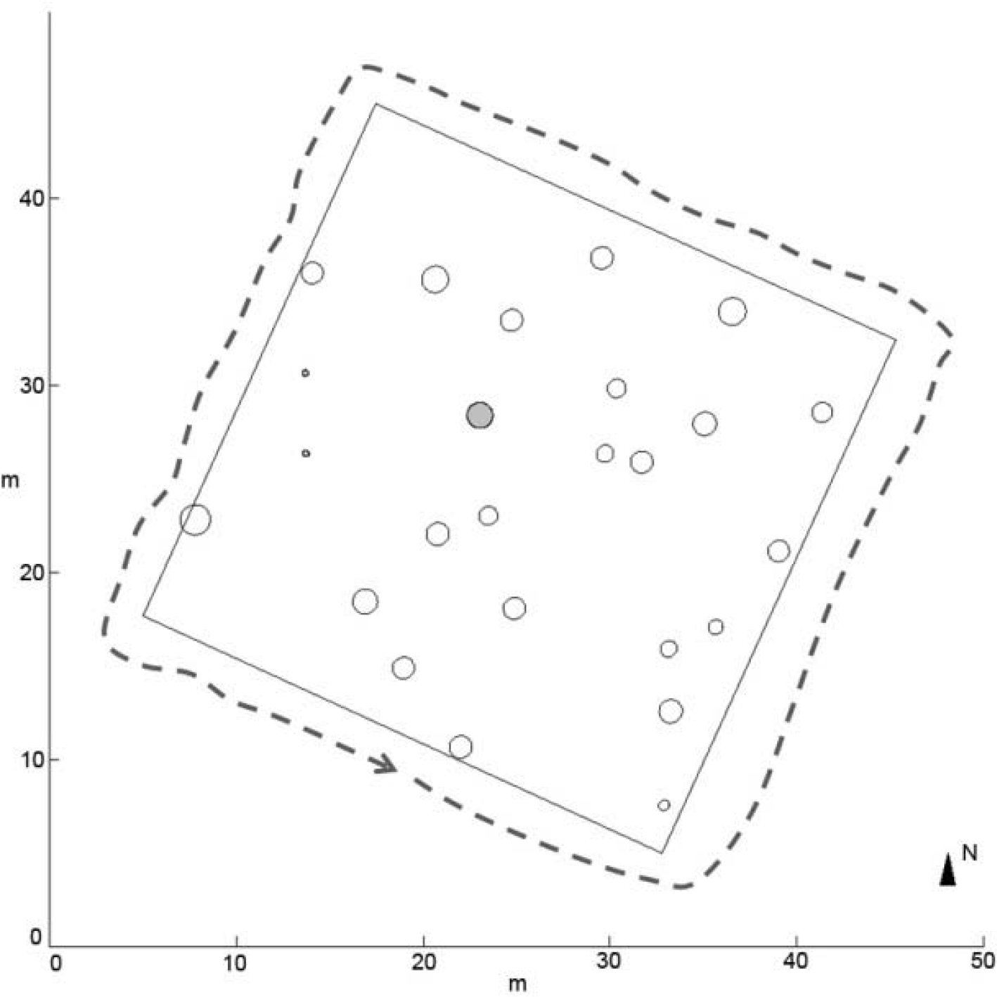
A stop and go mode was used to acquire photos. The operator took a picture at a photographing position and moved to the next position by a small step, e.g., 20 cm. The camera was held by an operator at approximately breast height, and a portrait image was taken from every photographing position. The camera was pointed towards the plot and the image plane was approximately parallel to the plot boundary. The photographing path was surrounding the plot, outside of the plot boundary, as shown in Figure 1.

The camera was not calibrated. The operational parameters were set to a F 7.1 aperture, a 1/125 second shutter speed and a 400 ISO value. Before the operation, the camera was manually focused. A large depth of field was set so that objects both near and far away from photographing positions would be clearly and sharply photographed. The image size was 5472 × 3648 pixels, and a total of 973 pictures were taken along the photographing path.

2.4. Other Field Measurements for the Image-Based Point Cloud

Two types of measurements were made in the field for reference information to determine the scaling factor of the image-based point cloud.

The first method measured the distance between tree pairs. Three tree pairs were randomly selected in the test plot. For each pair, tree trunks were marked with tape at approximate breast height, and the distance between two pieces of tape was measured utilizing a Leica Disto pro (Leica Geosystem AG, Heerbrugg, Switzerland) hand-held laser distance meter. The meter produced distance measurements at a 0.1 mm level. The distance between a tree pair was measured twice, from tree I to tree II and from tree II to tree I. The average of these two measurements was taken as the distance between the tree pair. The measured distances of the three tree pairs ranged from 6.34 m to 11.50 m and were utilized as the reference data from natural objects.

In the second method for determining the scaling factor, artificial reference targets were employed. Four sticks were set up in the south-west corner of the test plot to form three sets of reference data. An individual stick was laid on the ground, and its length was measured using a steel tape to the millimeter accuracy and taken as the first set of reference data. Two stick pairs were formed by the other three sticks vertically standing at the plot corner, with one stick standing at the plot corner point and the other two sticks standing approximate 5 m away from the corner point separately along the two conjunct plot borders. The distances between these two stick pairs were used as the second and third sets of reference data from artificial targets.

2.5. TLS Measurements

A TLS point cloud was also collected as a reference for the evaluation of image-based point cloud. The study area was scanned in April 2014 using a Leica HDS6100 TLS (Leica Geosystems AG, Heerbrugg, Switzerland). The distance measurement accuracy of the scanner is ±2 mm at 25 m distance and the maximum measurement range is 79 m. The scanner weights 14 kg. The dimension of the scanner is 199 mm in length, 294 mm in width and 360 mm in height.

The study area was scanned using the single-scan approach. A full-of-view (360 degrees by 310 degrees) scan was performed at the approximate plot center. The forest area was scanned as it was: no pre-scan preparations, such as the removal of lower tree branches or the clearance of undergrowth, were made.

3. Method

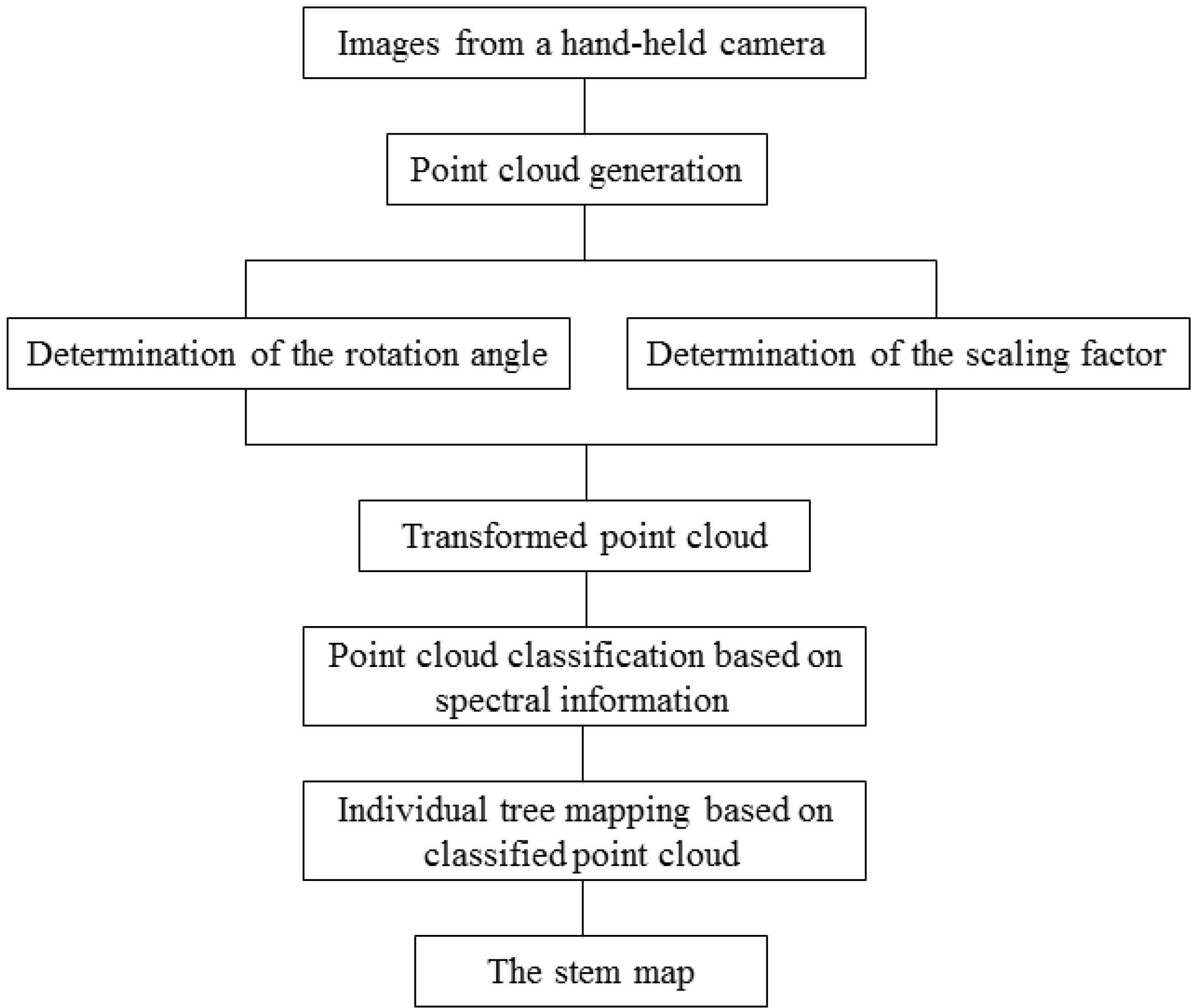
The flow chart of the data processing is shown in Figure 2. Three main steps include the point cloud generation, the point cloud transformation and the individual mapping using the image-based point cloud.

3.1. Point Cloud Generation

Point cloud data were generated utilizing the automated image matching procedure of Agisoft PhotoScan Professional commercial software (AgiSoft LLC, St. Petersburg, Russia). The quality parameter of the matching process was set to high, and an automated lens calibration was performed simultaneously. Point clouds were generated after image matching with the point density setting set to low. These parameters were selected considering the total amount and the size of the images (973 images, 5472 × 3648 pixel per image) as well as the computational capacity of the current software and hardware. The number of generated points was 8.0 million and it took approximately 32 h on a computer with a Intel Xeon E5-2630 CPU (six-core @ 2.3 GHz) and 32 GB of DDR3 RAM. During the point cloud generation, the assumption that consecutive images were close to each other was not made. Therefore, the number of image pairs to be tested was huge and the processing time was long. In cases that images are taken consecutively, such as in this experiment, such assumption can be made and the processing time is expected to be relatively short, e.g., several hours.

Two datasets were established based on the same point cloud data. The difference between two datasets was the spectral information derived from the images. Each point in dataset I had an additional spectral response in the green (G) channel, and each point in dataset II had three spectral responses in the red (R), green (G) and blue (B) channels.

3.2. Point Cloud Transformation

The point cloud generated from the images is in a camera space defined by the image matching procedure. Two transformation factors are required in order to obtain a 3D point cloud similar to what recorded by TLS, i.e., the rotating angle of the Z axis and the scaling factor. These two parameters can be retrieved using different methods. For example, points with known coordinates can be utilized to calculated transformation factors, which may be measured by a positioning instrument such as a Global Navigation Satellite System (GNSS) receiver. Another solution is to use camera locations recorded by a GNSS receiver to orientate and scale the image-based point cloud. The challenge for GNSS-based methods is that the positioning accuracy under tree canopies is typically degraded. This section presents the relationship between the camera space and real-world space, and discusses an alternative method for the retrieval of transformation parameters when a GNSS receiver or orientating function in a software package is not available.

3.2.1. Relationship between Camera Space and Real-World Space

The camera space is usually aligned with an initial image and is constantly adjusted according to the epipolar geometry of the found matching points in other images. At the end of the 3D reconstruction, the generated point cloud as well as the locations of the images/cameras are all registered in the camera space. Figure 3 illustrates the relationship between the camera space and the real-world space.

As shown in Figure 3, the camera space does not necessarily align with the real-world space. The direction of the Z axis of the real-world space may be rotated in the camera space depending on the camera orientation during the photographing procedure. The angle between the Z axis of the real-world space and the col axis of the camera space can be defined as the rotating angle R_z of the Z axis in the camera space, and R_z is free both on the (dep, col) plane and the (row, col) plane.

Another important relationship between the two spaces is the scale of the camera space with respect to the real-world space. In Figure 3, L_R is the cylinder height in the real world and L_c is that in the camera space. The scaling factor can be simply defined as the ratio between L_c and L_R.

To link the camera space to the real-world space, the rotating angle of the real-world Z axis R_z and the scaling factor must be determined.

3.2.2. Rotating Angle of the Z Axis

The operator kept the camera aligned with the real world during the image acquisition utilizing portrait image orientation. For the portrait images, col and row axes of the camera space are parallel with to X and Z axes of the real-world space. Therefore, R_z can be considered to be zero.

However, the alignment between the camera and the real world cannot be guaranteed, due to the misinterpretation of the camera orientation and the horizontal direction by the operator especially in a slope terrain. Although R_z can be reduced to a very small number by the best efforts of the operator, the rotating angle of the Z axis still exists. At this stage, no clear influence of this rotation angle was observed.

3.2.3. Scaling Factor

As described in Section 3.2.1, the scaling factor λ can be defined as follows:

$$\lambda =d_{\mathit{data}}/d_{\mathit{field}}$$

(1)

where d_field is the distance between two known points in the real-world space, e.g., the distance between two reference points measured in the field; d_data is the distance between two corresponding points of field reference points in the camera space.

Two methods were applied for the determination of λ (ref. Section 2.4). The first method measured the distance between selected tree pairs in the test plot as d_field. The second method collected d_field measurements utilizing artificial targets. The main purposes of applying these two methods were: (1) to verify the consistency of the λ measurement at different locations in the image-based point cloud; and (2) to evaluate the necessity of artificial targets for determining λ.

To determine λ from tree pairs, three tree pairs in the test plot were selected, and stems of the measured tree pairs were marked with tape. The distance d_field between tree pairs were measured in the field, and the corresponding distance d_data were measured in the image-based point cloud. A slice was cut from the point cloud through the pieces of tape around the stems. In this slice, stem points were selected and the distance d_data was measured. The generated point cloud of one tree was too sparse to identify stem points, which made the distance measurement of a tree pair in the point cloud impossible. The scale factor of the point cloud was the average of the λ values from the other two valid tree pairs.

With the artificial targets, the length of a single stick lying on the ground and the distances between two vertically placed stick pairs were measured both in the field and in the image space, and other λ values were also derived from the reference targets.

The results showed that the scaling factor λ can be calculated at different locations in the point cloud, and λ values derived from the natural and artificial targets were similar. The scaling factor determined based on the tree pairs was utilized in the data processing because it does not require additional reference objects and therefore is easy to perform in the field. This actually indicates that artificial reference targets are not necessary in practical operations.

3.3. Individual Tree Mapping

A two-stage procedure was applied for individual tree mapping in a sample plot from a terrestrial image-based point cloud. Firstly, only the spectral information of each point was employed to roughly classify objects in the plot: tree stem, tree crown and ground. Uninterested points, e.g., points of ground and tree crown, were eliminated so that the subsequent tree stem mapping step could focus on valuable information. Secondly, tree stems were detected and modeled based on the spatial information, i.e., the XYZ coordinates of the points.

3.3.1. Point Classification

Objects in the test forest plot were roughly grouped into three categories: tree stem, tree crown and ground. At the time of image data acquisition, these three categories had clearly different spectral responses: the tree stem had a low value in the G channel; tree crown had a high value in the G channel; and ground was covered by snow and had a high value in all RGB channels.

According to different spectral responses of different objects in the test plot, an automated K-means clustering with fixed group number was applied to classify the points of tree stem, tree crown and ground.

The K-means method partitions dataset P into K clusters, such that the sum of squared distance E is minimized, as shown in Equation (2).

$$E={\sum }_{i=1}^K{\sum }_{p\in C_i}{(d(p,c_i))}^2$$

(2)

where p is a point in cluster C_i, i = 1,2, ⋯, K, c_i is the center of the cluster C_i and d is the distance between point p and c_i.

The spectral information of the points retrieved from the images was noisy because of inaccurate matching and illumination conditions as examples. Objects in the same categories may present wide variances in spectral responses. Although there were only three classes, it was challenging to group the points into exactly three clusters due to noise.

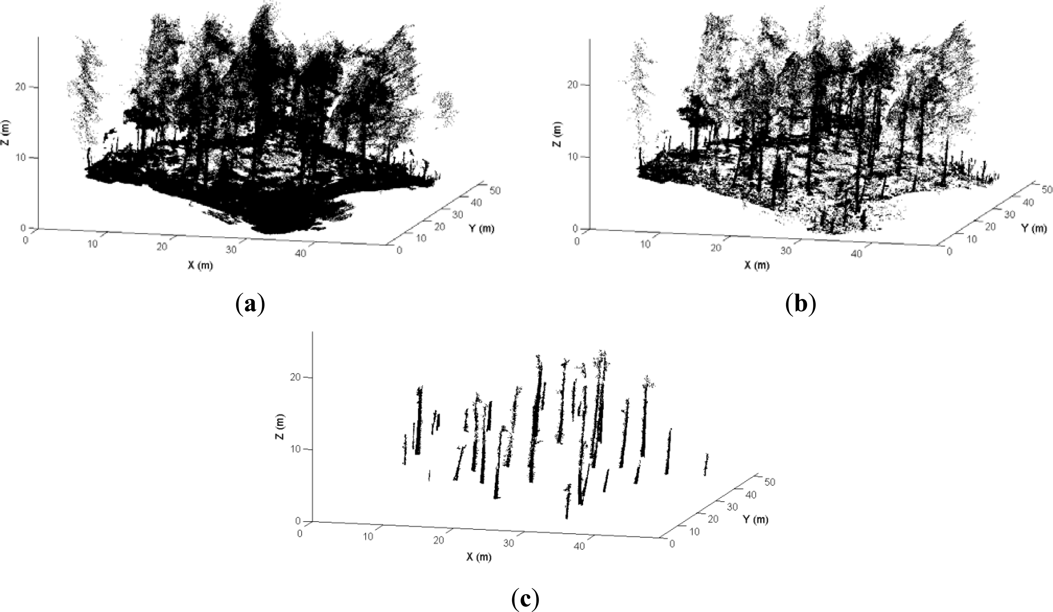
To reduce the influence of noise, the cluster number K was doubled to six for both datasets, and the cluster number of each category was doubled to two. In dataset I, a one-dimensional K-means classification was applied. Two clusters with the lowest mean G value were classified as tree stems. There were 2.6 million selected points and 8.0 million points in the original point cloud data. In dataset II, clustering was performed in three dimensions. Two clusters with the highest mean value in the RGB channels were considered to be ground because the ground was covered by snow. The ground points were eliminated from the point cloud. The subsequent tree stem detection was based on the rest of the points, which accounted for 6.2 million of the 8.0 million in the original data.

3.3.2. Individual Tree Mapping

Classified points were further processed utilizing a robust tree mapping method [18]. Stem points were first identified from the point cloud based on their spatial distribution properties. Each point was automatically processed in its neighborhood, and the size of the neighborhood was determined based on the local point density; the higher the local point density, the smaller the size of the neighboring space, and the lower the local point density, the larger the size of the neighborhood. In this study, the neighborhood is defined by k-nearest points (k = 100).

A local coordinate system was established for each point in its neighboring space. The axis directions were indicated by the eigenvectors, and the variances of the points along the axes were given by eigenvalues. A stem point is typically on a vertical planar structure. The planar surface was identified based on the distribution of the neighboring points if they were mainly along two axes in the local coordinate system. The vertical shape was recognized based on the normal vector to the surface, which was approximately horizontal in the real-world coordinate system.

The tree stem models were built from these possible stem points. A series of 3-D cylinders were utilized to represent the changing stem shapes. As noise was still present, e.g., the branch points, each point was weighed to reduce the noise influence. The DBH and location of the stem were then estimated from the cylinder element at the breast height.

Figure 4 presents the original point cloud of dataset I (a), the classified dataset with low green values (b), and the detected stem points (c).

3.4. TLS Point Cloud Processing

TLS data within the study area was sampled by every nth point so that the amount of the TLS points in following data processing (7.8 million) is similar to that of image-based points (8.0 million). The n was 4 in this experiment. This TLS data was referred as data set III in following and was utilized as a reference set to evaluate the accuracy of tree-attribute estimates from image-based point clouds.

TLS data set was processed utilizing the robust modeling method (described in Section 3.3.2) to estimate tree attributes.

3.5. Evaluation Criteria of Tree Mapping Results

The tree mapping results were evaluated using the measured references in the field. The mapping accuracy was evaluated based on the omission errors, commission errors and overall accuracy. Overall accuracy is the percentage of correct detections.

The accuracy of the DBH and position estimates were evaluated utilizing the bias and RMSE, as defined in Equations (3) and (4):

$$\mathit{Bias}=\frac{1}{n}\sum _{i=1}^n{e}_i=\frac{1}{n}\sum _{i=1}^n(y_i-y_{ri})$$

(3)

$$\mathit{RMSE}=\sqrt{\frac{\sum {(y_i-y_{ri})}^2}{n}}$$

(4)

where y_i is the ith estimate, y_ri is the ith reference, and n is the number of estimates. Relative bias and RMSE were also employed to evaluate the mapping result, which were calculated by dividing bias and RMSE by the mean of the reference values.

4. Result

The results of the tree mapping utilizing image-based and TLS point clouds are reported in

Table 1. Tree mapping accuracies of image-based point clouds.

		Reference	Mapped	Omission	Commission
I	Number (stem)	25	22	3	3
	Percentage (%)	100	88	12	12
II	Number (stem)	25	22	3	4
	Percentage (%)	100	88	12	16
III	Number (stem)	25	22	3	1
	Percentage (%)	100	88	12	4

. The omission errors were reference trees that were not mapped, and the commission errors were detected trees without corresponding reference data. Dataset I and II produced an overall detection accuracy of 88 percent.

Omission errors of both image-based datasets were located in the middle of the sample plot, where points were sparse and noisy. The first reason for this is that the trees in the middle of the plot were far from the photographing path so that the identification of the image correspondences and the retrieval of 3D geometry were less accurate. The second reason is that two omission errors in both datasets were young trees that measured just above 10 cm DBH, which shows that the image-based point cloud most probably has limited capacity to capture young trees with small DBHs.

The commission errors of both image-based datasets were from saplings and small trees. Their estimated DBHs were exaggerated because of the noisy point data and therefore they were falsely detected as tree stems.

Detecting results from the single-scan TLS data was similar to the image-based datasets. Omission errors include two trees partially occluded by other tree stems which standing closer to the scanning position. The third omission error was a small tree (one of two young trees that were not detected from image-based point clouds). It was surrounded by saplings and bushes, and therefore the stem was not successfully modeled. These three omission errors were recorded in the TLS point cloud and stem points of the existing parts were also successfully detected. But, the stems were not modeled because of the undergrowth and the occlusion effects. The commission error of the TLS data set was a young tree with a DBH close to 10 cm.

The accuracies of the DBH and the position estimates for the detected trees of two image-based and TLS point clouds are reported in

Table 2. The accuracy of the DBH and position estimates utilizing image-based and TLS point clouds.

		Bias	Bias%	RMSE	RMSE%
I	DBH (cm)	0.48	1.33	2.39	6.60
	Position (m)	0.12		0.14
II	DBH (cm)	1.98	5.39	4.47	12.14
	Position (m)	0.12		0.14
III	DBH (cm)	−0.58	−1.66	2.55	7.27
	Position (m)	0.05		0.06

.

5. Discussion

This experiment proved the applicability of the image-based point cloud from an uncalibrated hand-held camera for individual tree mapping in a forest plot. A point cloud that covered the whole forest plot can be generated from a set of images taken around the plot. The originally generated point cloud does not geometrically correspond to the forest scene, or the geography coordinate system. It was in a camera coordinate system defined in the image matching procedure. The methods to align the two coordinate systems were proposed and studied. The accuracy of the tree-attribute estimation from image-based point clouds was evaluated using both field reference data and the estimation accuracy from a TLS point cloud.

The result of this study showed that DBHs and locations of trees within the forest plot can be estimated from image-based point clouds at an acceptable level for practical field inventories. The accuracy of the DBH estimation using TLS is expected to be better than that of the image-based point cloud. In this experiment, however, the accuracy achieved from image-based point clouds was similar to what derived from the TLS data. The performance of the single-scan TLS in this test was affected by the occlusion effects introduced by other objects standing closer to the scanning position. The lower part of a tree stem was totally occluded by another tree stem which brought a cross error of the DBH estimation. The RMSE of DBH estimates would be 1.98 cm if that cross error had been excluded from the evaluation. The utilization of multi-scan TLS data will most probably improve the estimation accuracy since tree stems are scanned from different directions and the occlusion effects are minimized. This, however, requires the registration of several scans, which is still semi-automated at this moment. Besides the stem modeling method utilized in this study, there have been several developments on other methods for stem modeling, such as the RANSAC circle or cylinder fitting [14,19] and least square circle fitting [6]. These methods may also be utilized in the image-based point clouds.

The equipment required to generate image-based point clouds are much lighter, cheaper and easier to operate than TLS. For example, the camera used in this experiment weighs 420.8 g and costs several hundreds of euros; the TLS weights 14 kg and costs several tens of thousands euros. The lightest scanner currently available in the market weighs only 5 kg. The weight and cost of TLS instruments in coming years will most probably further decrease. However, in foreseeable future, a consumer camera will still be cheaper and lighter than an active sensor that produces point cloud data.

A weakness of the image-based point cloud is the lack of capability to penetrate small branches and leaves in comparison with TLS. Therefore, the use of image-based point cloud in dense forests would most probably meet difficulties, such as tropical forests. This also applies to certain tree species, such as spruce trees, which have a lot of branches and leaves around their stems. The image-based point cloud is likely to be a practical technique in boreal or well managed forests where the lower vegetation layer is sparse. In addition, the operational range of the image-based point cloud is quite limited. Research has shown that TLS can map tree stems up to 30–60 m [5,7,9,20,21].

The image-based point data also require more efforts to produce a point cloud in comparison with TLS. For a dataset with several hundreds of images, the image matching and point generation often take a lot of time, e.g., several hours. The TLS point cloud data are, however, ready for use just after the field data collection, which makes fast data processing possible. The efficiency of applying image-based point cloud in practical forest inventory needs more studies.

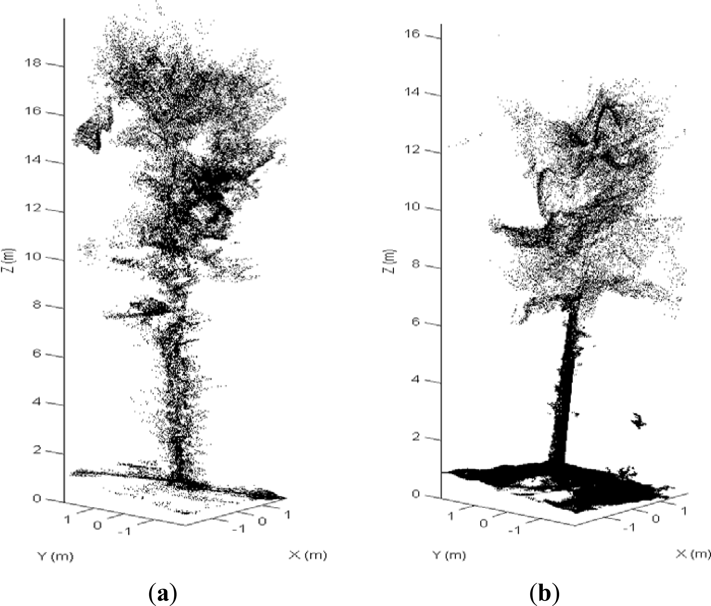
The density and the geometric accuracy of points varied in an image-based point cloud. Figure 5 illustrates the points of two trees from dataset I. A 43-cm DBH Tree A in Figure 5a was located near the plot center and was approximate 20 m from the photographing path. A similar Tree B in Figure 5b was approximately 5 m from the photographing path. The sparse and noisy points of tree A are the results of the inaccuracies in the camera calibration and image matching as well as the longer distance of tree A from the photographing path. Another reason could be the unfavorable lighting condition within the forest. In the experiment, the plot was photographed using a relatively slow shutter speed (1/125), which might reduce the sharpness of objects at a longer distance from the photographing path.

The quality of the image-based points was largely dependent on the distance of the object from the photographing path. The closer an object was to the photographing path, the better the performance of the point cloud generation. Tree A was detected but was not modeled due to the low quality of the point cloud at its location. These results show that for successful detection and modeling of tree stems, a 15 m distance is most probably the maximum distance between a tree and the photographing path. The size of a sample plot is also closely related to the canopy structure of the plot. For a dense plot, the size of the plot should be smaller.

The accuracy of the scaling factor is crucial for the utilization of an image-based point cloud for sample plot mapping at the individual-tree level. Two methods were tested for the determination of the scaling factor. The results showed that both natural reference objects and artificial targets worked effectively. Artificial targets are relatively easy to identify in images but need extra equipment. The utilization of natural reference objects, e.g., tree stems, is convenient. However, measuring the distance of objects in the generated point cloud can be challenging when the reference objects were presented by sparse and noise points or were even absent from the image-based point cloud.

This experiment also demonstrated the usability of spectral information in an image-based point cloud for object classification. The spectral-based classification significantly reduced noise and redundant points, which is beneficial for both tree mapping efficiency and DBH estimation. The DBH estimates in dataset I were more accurate than those in dataset II, which demonstrated that the elimination of noise around the stems improved the stem modeling accuracy using image-based point cloud.

Snow-covered ground may be an exceptional case in many regions. The classification of ground points in this study is an example of applying spectral information of the image-based point cloud in object recognition. Further studies are needed to explore the potential of utilizing spectral information in, e.g., species classification.

Conventional instruments, such as the relascope, are handy, inexpensive and reliable for measuring basal area. Stem locations may also be measured rather quickly using instruments such as the laser relascope or even a rangefinder and a bearing compass. The real advantages of point-cloud data, for both TLS and image-based, come from deriving advanced tree attributes, such as an accurate stem curve.

Compared with previously developed imaging systems, which require specific instruments and individual tree measurements in the field, the utilization of image-based point cloud is convenient and highly automated. Only a hand-held camera was required for the data collection, and calibration of the camera was unnecessary. In this experiment, the photographing required approximately 43 min for the plot, and only a few simple field measurements were required.

6. Conclusions

This paper analyzed a new image-based approach of individual-tree mapping in forest plots using a low-cost consumer camera. A series of densely-overlapped portrait images were photographed around the sample plot using an uncalibrated hand-held camera. A point cloud was generated from these images, and was later transformed from a camera space to the real world space. Individual tree stems were automatically detected and modeled based on both spectral and spatial information captured in the point cloud. The results show that current terrestrial image-based point clouds are capable of providing a 88% mapping accuracy and a 2.39 cm RMSE of DBH estimates of individual trees in a 30 × 30 forest plot, which is similar to the results achieved using single-scan TLS and is acceptable for practical applications.

The main advantages of image-based point cloud data are the low cost of the equipment needed for the data collection, the simple field measurements and the automated data processing. The requirement of additional investment for equipment or external expert knowledge is minimized. The disadvantages include the difficulties of mapping small trees and complex forest stands. However, for complicated cases, semi-automated processing can be an option for improving the mapping accuracy.

Further studies are needed to determine the accuracy of stem curve estimation using image-based point cloud data, the possibilities of applying different image-collection strategies and setups in the field and the influence of camera quality.